GRID: A Python Package for Field Plot Phenotyping Using Aerial Images

Abstract

Aerial imagery has the potential to advance high-throughput phenotyping for agricultural field experiments. This potential is currently limited by the difficulties of identifying pixels of interest (POI) and performing plot segmentation due to the required intensive manual operations. We developed a Python package, GRID (GReenfield Image Decoder), to overcome this limitation. With pixel-wise K-means cluster analysis, users can specify the number of clusters and choose the clusters representing POI. The plot grid patterns are automatically recognized by the POI distribution. The local optima of POI are initialized as the plot centers, which can also be manually modified for deletion, addition, or relocation. The segmentation of POI around the plot centers is initialized by automated, intelligent agents to define plot boundaries. A plot intelligent agent negotiates with neighboring agents based on plot size and POI distributions. The negotiation can be refined by weighting more on either plot size or POI density. All adjustments are operated in a graphical user interface with real-time previews of outcomes so that users can refine segmentation results based on their knowledge of the fields. The final results are saved in text and image files. The text files include plot rows and columns, plot size, and total plot POI. The image files include displays of clusters, POI, and segmented plots. With GRID, users are completely liberated from the labor-intensive task of manually drawing plot lines or polygons. The supervised automation with GRID is expected to enhance the efficiency of agricultural field experiments.

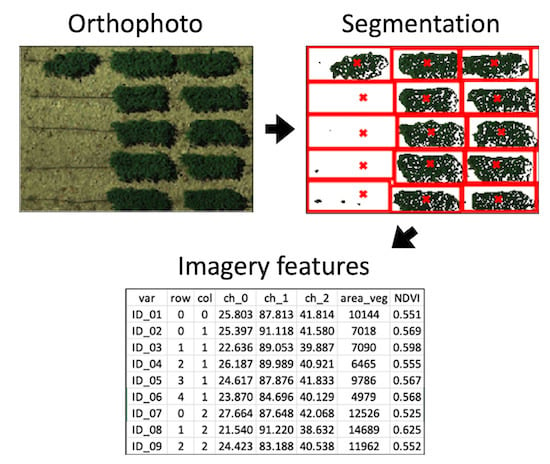
1. Introduction

Agricultural field experiments have an advantage over greenhouse experiments because environmental conditions in the field are closer to real-world situations. The disadvantages of open-field experiments are the massive scale; unpredictable influence of natural forces; and expensive and labor-intensive manual phenotyping, which often requires traveling long distances and enduring harsh working conditions. Remote sensing technology, on the other hand, has the potential to improve in-field phenotyping efficiency [1]. That is, remotely sensed images can partially substitute for manual phenotyping in a high-throughput manner, or even include additional plant characteristics not possible to collect through manual phenotyping.

To record and utilize such characteristics from field experiments, orthoimages can serve as the digital media for transferring the information. This type of image is acquired from satellites or unmanned aerial vehicles (UAV), having been adjusted for lens distortion and camera tilt. Practically, orthoimages are saved in Geographic Tagged Image File Format (GeoTIFF). This file format can record more than three imagery channels, allowing scientists to explore information beyond visible wavelengths, such as near-infrared (NIR). GeoTIFF can also embed geographical information into orthoimages. To use these images for field experiments, plot boundaries must be defined for segmentation, and the pixels of interest (POI) must be extracted. During the image process, several roadblocks prevent the use of orthoimages for high-throughput phenotyping for agricultural experiments.

The first roadblock is a lack of ground devices for geographical information in the majority of orthoimage applications. Efforts have been made to ease this difficulty. One example is QGIS [2], which has a graphical user interface (GUI) and comes with versatile toolsets, enabling users to dissect terrain [3,4] or time-series variation [5], visualize raster data [6,7], and export the derived information for further applications. For applications without geographical information, QGIS allows users to either specify an area of interest (AOI) by manually drawing polygons or assign pixels as reference. Then, the software can identify pixels that share a similar spectral pattern. However, implementing segmentation in such a way can be time-consuming and laborious because one must manually draw the polygons around plots being investigated.

To overcome the second roadblock of manually drawing polygons and assigning reference pixels, image segmentation tools have been developed to eliminate the labor by utilizing the grid layout of agricultural experimental fields. Field plots are commonly organized in grid layouts with rectangular, rhombus, or parallelogram patterns. Hence, by having essential parameters (e.g., size of plot, number of rows and columns) that define the field arrangement as guidance, plots can be automatically segmented if plots are aligned properly. Progeny [8] and EasyMPE [9] implemented this method to allow users to define plots without drawing polygons. The challenge is that plots are often misaligned between one row and another.

To deal with the third roadblock of misaligned field plots, the Phenalysis program [10] was developed to adjust plot centroids using particle swarm optimization [11]. The algorithm arbitrarily initializes plot centroids and iteratively updates their locations based on the cost function, which is defined by intra-plot and inter-plot vegetation indices. The centroid locations are optimized when the function value converges or satisfies the criterion.

The fourth roadblock is the extraction of AOI within plot boundaries. Trainable Weka Segmentation (TWS) [12] is a segmentation tool that comes with a supervised learning algorithm and learns pixel-based features from a provided training dataset. TWS can classify any pixel from given images. As the common disadvantage of supervised learning algorithms, the training process itself is labor-intensive. Additionally, this type of algorithm experiences difficulty when images contain objects that are outside the training range. Images of agricultural fields are extreme challenges for training. For example, plants can grow across their neighboring plots so that leaf canopies connect with or overlap each other. Irrelevant objects appear in a variety of forms, such as weeds and drip irrigation pipes.

Among the existing methods and software packages, none of them simultaneously fixed these roadblocks and satisfy all desirable features to efficiently analyze images for plot information, including (1) independence from ground devices for geographical information, (2) freedom from drawing lines or polygons, (3) tolerance to plot variation due to plant interaction within and between plots, and (4) usability with minimal training. In this study, we developed automated methods and a software package to achieve all of these features, requiring little user guidance and including an easy-to-operate, interactive GUI. When users slide control bars on the GUI, results are instantly displayed for adjustment so that users can integrate their knowledge about the experimental fields into the final results. The package, named GReenfield Image Decoder (GRID), was designed by PyQT5 [13] and managed by Python Package Index.

2. Methods

2.1. Workflow

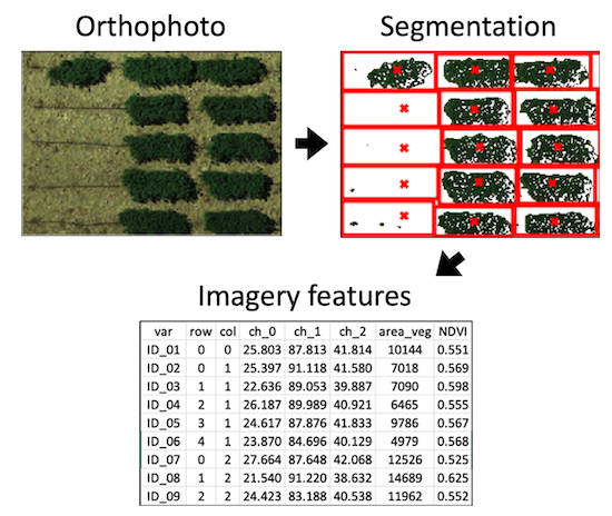
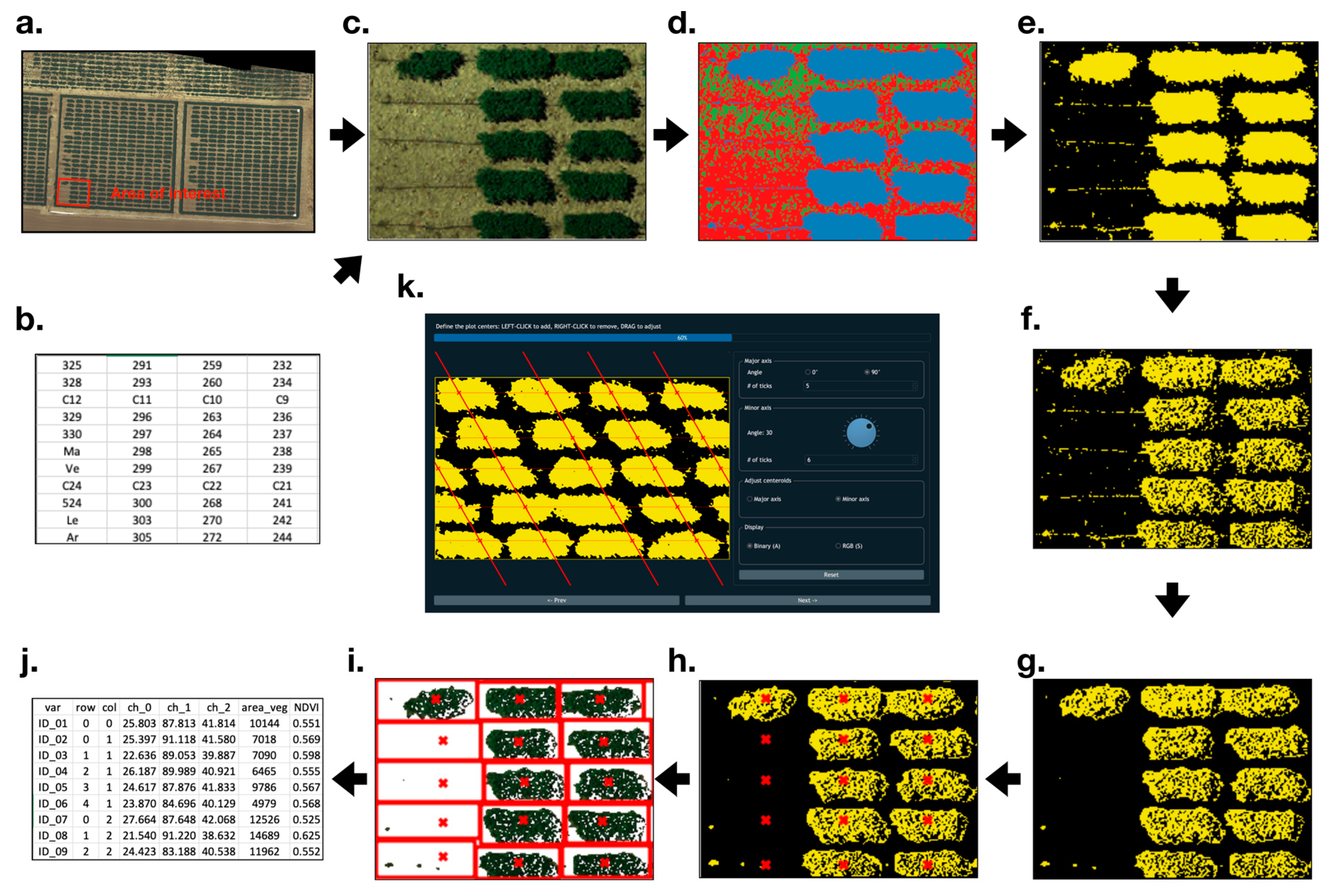
GRID is initiated by prompting the user for an input image (Figure 1a) and an optional map file (Figure 1b). The map file contains the identification of plots that are arranged in rows and columns. The number of rows and columns also serves as the default to guide the segmentation. Without the map file, GRID automatically infers the layout from the image. For the input image, users can either keep the original scope or assign four corners to crop a rectangular area for segmentation (Figure 1c). To differentiate pixels of interest (POI) from the background, a pixel-wise clustering is carried out (Figure 1d). POI and background pixels are labeled as 1 (highlighted in yellow) or 0 (black), respectively, to form a binary image (Figure 1e). The binary image can be further refined by shade removal (Figure 1f) and noise removal (Figure 1g). Based on the distribution of POI in the image, GRID can infer the field layout and locate plot centers via signal analyses (Figure 1h). The determined plot centers are used as starting points to initialize an intelligent agent. Agents will bargain with their neighboring plots and expand the plot boundaries (Figure 1i). Detailed algorithms of all the above steps are elaborated in the later sections. Each step in GRID comes with friendly graphical user interface (GUI) components. Users are allowed to fine-tune parameters via simple actions, such as dragging slider bars or clicking a mouse, and the final results are updated in real time. The segmentation results are saved as text in comma-separated values (CSV) files with CSV extension names (Figure 1j) and are visualized in Portable Network Graphics (PNG) images. The text files include plot rows and columns, plot size, and total plot POI. The image files include displays of clusters, POI, and segmentation results. Other than text and image files, a binary file is generated along with the analysis. This file, with the extension name “.grid”, records all optimized parameters from the segmentation, and users can load it into GRID to replicate the analysis on other images.

2.2. Input Images and Field Layout

GRID supports most image formats, including GeoTIFF, PNG, and Joint Photographic Experts Group (JPEG). All the channels from the image are loaded as a 3-D array (i.e., width by height by channels), which later serves as numeric features for pixel-wise clustering. By default, GRID assumes the first three channels from the input image are red, green, and blue, respectively. If the image has more than three channels, GRID considers the fourth channel as near-infrared (NIR), but it does not make presumptions for any additional channels. To accelerate the computing speed, the input image is encoded to Uint8 and is proportionally resized to a smaller copy. The longest side of this copy is shorter than 4096 pixels and is used to represent the original image for the entire analysis. The image loading function is implemented by Python Rasterio [14], and the 3D array is managed by a numpy array [15].

A map file is an optional input into GRID and should be saved as a CSV file. Recorded in the file are tabular data, which represent the field layout. For example, if the image contains five columns and three rows of plots, the table should also have five columns and three rows of data cells. Values in the data cells are the plot names given their positions in the field. The names are also shown in the output file and allow users to track the specific plot. In general, providing the map file gives GRID a better idea of how many plots exist in the image and results in a better segmentation with the default configuration. However, if no map file is provided, GRID can still determine the field layout, but with less accuracy.

2.3. Perspective Correction

An orthomosaic is the most common input image format in phenomics. An orthomosaic is generated from merging several small orthoimages to cover a wide range of areas and has already been corrected for lens distortion and camera tilt. However, the correction cannot ensure that the selected AOI from an orthomosaic is in the shape of a rectangle; usually, an observable distortion remains in the image. To alleviate this problem, GRID linearly transforms and maps the current AOI into the shape of a rectangle. The four corner coordinates (x_i, y_i) from the AOI are defined as corresponding points P. A homography H can be found in the following equation:

$${\rm P}{H}^T= \left[\begin{array}{ccc}{x}_1& y_1& 1\\ x_2& y_2& 1\\ x_3& y_3& 1\\ x_4& y_4& 1\end{array}\right]·{\left[\begin{array}{ccc}x{h}_{11}& y{h}_{12}& h_{13}1\\ x{h}_{21}& h{y}_{22}& h_{23}1\\ x{h}_{31}& h{y}_{32}& h_{33}1\end{array}\right]}^T= \left[\begin{array}{ccc}{x}_1{}^{\prime }& y_1{}^{\prime }& 1\\ x_2{}^{\prime }& y_2{}^{\prime }& 1\\ x_3{}^{\prime }& y_3{}^{\prime }& 1\\ x_4{}^{\prime }& y_4{}^{\prime }& 1\end{array}\right]= P{}^{\prime }$$

(1)

where P′ equals the known four coordinates (x′_i, y′_i) that correspond to the four corners of the new projective rectangle. Therefore, the homography allows GRID to remove the distortion by applying such a transformation to the original AOI. The equation solving is implemented by the function getPerspectiveTransform () from OpenCV [16].

2.4. Pixels of Interest (POI)

GRID conducts a pixel-level segmentation for each plot. The red and NIR channels (or the red and green channels if the image has only 3 channels) are considered as numeric features, which are used in a pixel-wise clustering to identify POI (denoted as 1) and background (denoted as 0). Pixels are grouped into clusters. Users can decide which clusters belong to POI. The clustering is conducted via a k-means clustering algorithm. The number of clusters is set to three by default, corresponding to the three major types of objects existing in the field images: vegetation, soil, and the rest. The first-ranked cluster (vegetation most of the time) is selected as POI by default. Depending on the circumstance, users can freely tune the parameters, such as selecting imagery channels used for the clustering, number of clusters k and clusters specified as POI. The determination of POI turns the input image into a binary 2D matrix B, which consists of 0s (background) and 1s (POI).

The binary image B can be refined via two approaches: de-shade and de-noise. Since every orthophoto cannot be taken at noon—the time of day with the minimum amount of shadow—removing dark, shaded areas observed beneath the leaf canopy is essential for accurate analysis. The average of the first three channels (RGB) is used as a darkness (shade) indicator S_xy for a pixel at the coordinate (x, y). If we let M_xyi stand for the ith channel value at the pixel, the darkness of the pixel can be calculated as:

$$S_{xy}={{\displaystyle \sum }}_{i=1}^3\frac{M_{xyi}}{3}.$$

(2)

The corresponding values of the binary image at the coordinate B_xy is determined by S_xy and a threshold S_t:

$$B_{xy}=\{\begin{array}{c}1, if S_{xy}<S_t\\ 0, otherwise\end{array}.$$

(3)

Users can then filter any pixel darker than a chosen threshold S_t.

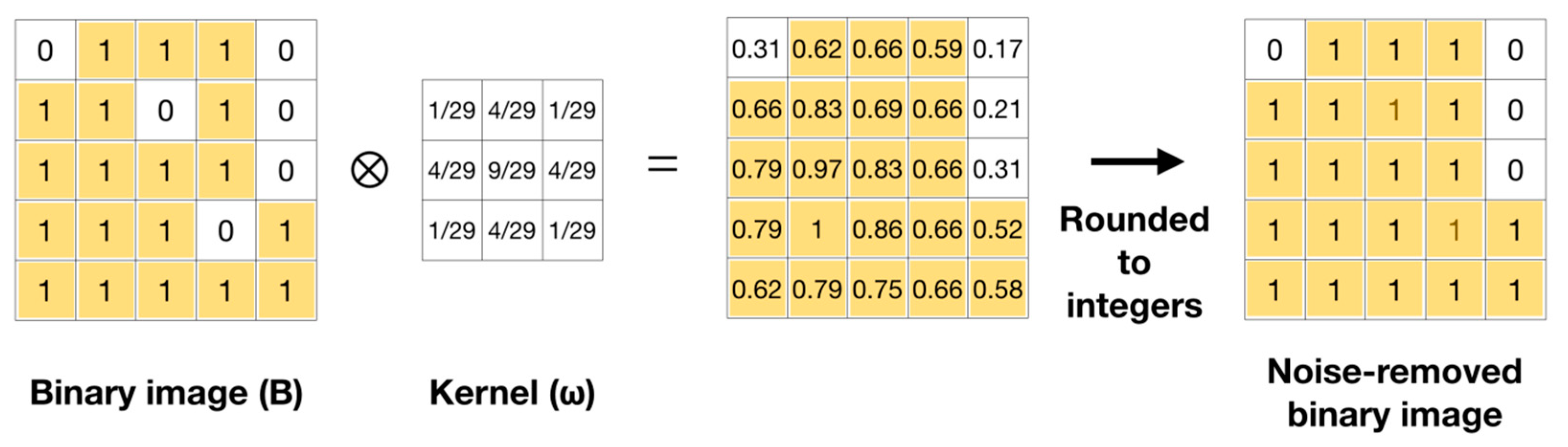
The other image-refinement approach is to smooth noise signals. In the field, many non-vegetation and trivial objects can be observed. For instance, pipes used for drip irrigation are usually placed under plant canopies and should not be considered part of the plant. Hence, GRID performs a 2D convolution operation to alleviate such noises. A pre-defined 3 by 3 kernel, ω, will span over the binary image B to smooth noises (Figure 2). A K-means clustering algorithm is implemented by OpenCV library, and the convolution operation is conducted via Python Numpy.

2.5. Plot Centers and Layout

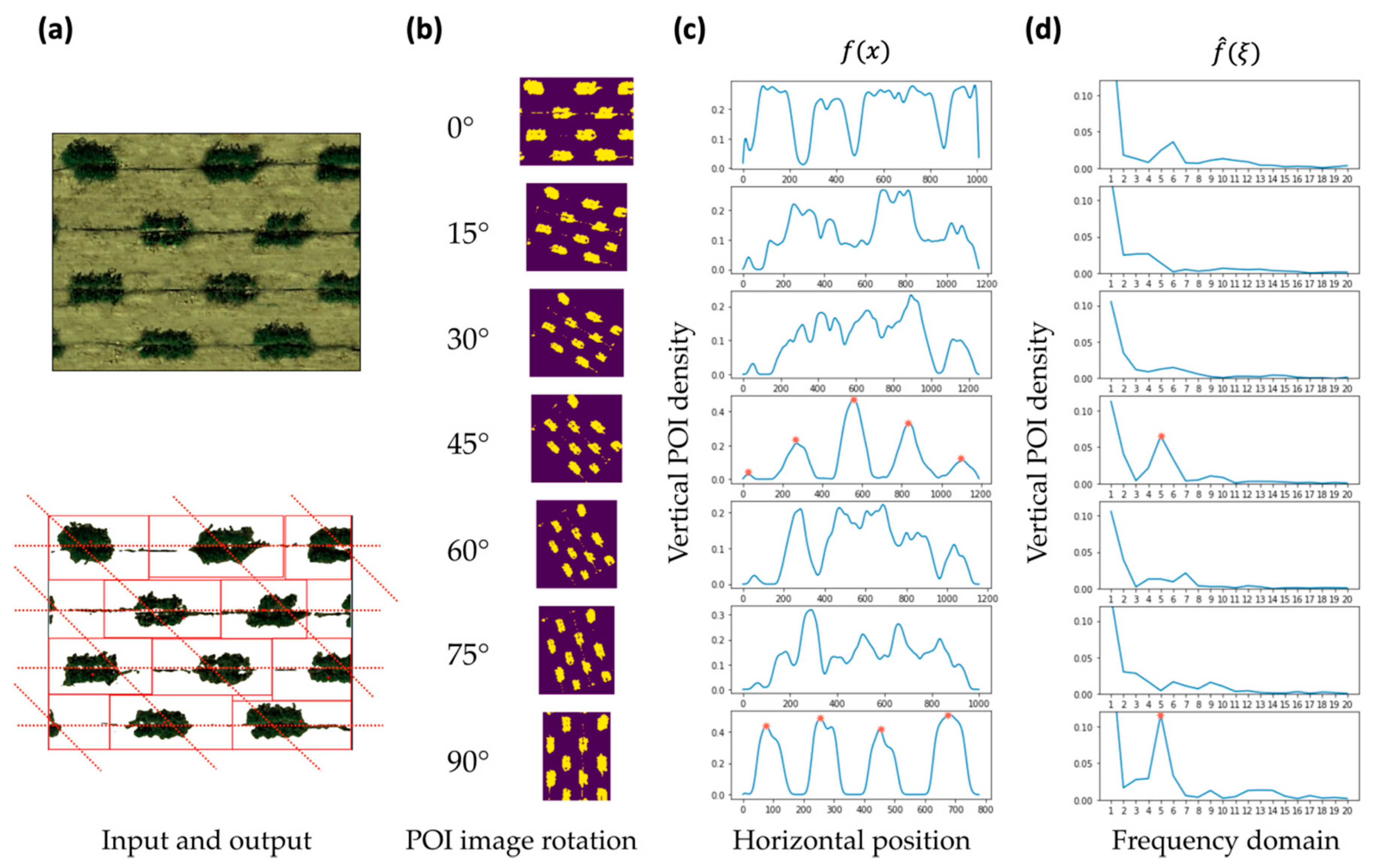
The binary image B defined from the previous step is used to determine plot centers and layouts. Plot layouts refer to how the plots are arranged. For most cases, plots are arranged in a grid pattern, where all rows and columns are perpendicular to each other. However, in some circumstances, the angles between rows and columns are less than 90 degrees, and drawing a simple grid is unlikely to accurately segment each plot from an orthoimage. To solve this problem, we must determine the angle between rows and a vertical line, and the angle between columns and a vertical line. We define these two angles as the “rows angle” and “columns angle”.

Fourier transformation, a math approach that finds constituent frequencies of given signals, is introduced to find the angles. The signal f(x) is a function of x coordinates from the binary image B:

$$f\left(x\right)={\displaystyle \sum }_{y=1}^h{B}_{xy}$$

(4)

where h is the height of the image. We can learn the signal frequency domain $\widehat{f}\left(\xi \right)$ via Fourier transformation:

$$\widehat{f}\left(\xi \right)={{\displaystyle \int }}_1^{w}f\left(x\right)e^{-2\pi ix\xi }dx$$

(5)

where ξ is the signal frequency, and w stands for the width of the image.

To search for the rows/columns angle, the binary image B is rotated clockwise from 0 to 90 degrees at 15-degree intervals. Each angle has a corresponding signal and f is defined in Equations (4) and (5) above. We use the maximum value of f to represent the periodicity of the signal. Signals having stronger periodicities have a higher chance that their corresponding angles match the rows/columns angle. The corresponding angles of the two signals with the highest periodicities are compared. The angle closest to 0 degrees is assigned as the columns angle, and the other is assigned as the rows angle. By knowing the field layout, we use the local optima of the signals defined in Equation (4) to locate plot centers. Signal values are compared with their neighboring values. If the location has a relatively higher value than those adjacent, the location is a local optimum and is defined as plot center of the corresponding row/column (Figure 3). Finally, combining the information of plot centers and field layout, GRID determines 2D coordinates of all the plots. Fourier transformation is implemented by Python numpy, and the local optima searching algorithm is realized via Python Scipy library [17].

2.6. Plot Boundaries

Before determining all plot boundaries, the dimensions of each plot must be estimated. An “intelligent agent” is initialized at the center point of each plot (defined in the previous step), and then it starts to traverse toward the four different cardinal directions (i.e., north, east, south, and west). Whenever the agent arrives at a new pixel position, it will examine whether this pixel is assigned to the POI or not. If yes, the agent will continue its traverse in the same direction to the next new pixel position. If no, the traversing will also continue in the same direction, but a 1+ increment will be added to the counter. The searching process in one direction is terminated when the counter becomes greater than the criterion. By default, the criterion is set to 5. With the information about how far an agent traveled in each direction, GRID can roughly estimate the width and length of each plot.

Each agent will bargain with its neighboring agents to expand its territory (Figure 4). The idea “bargaining bar” is introduced in this step. When the agent bargains with its horizontal (or vertical) neighbor, the bargaining bar is initialized as a vertical (or horizontal) vector at its plot center. The length of the vector is plot height (or plot length) estimated from the previous step. Two neighboring bars will iteratively compare their “bargaining power” to decide which one can shift a pixel toward the opposite plot. In the case of a tie, both bars can shift. This bargaining process will end when two bars meet at the same position, which is the position where plot boundaries are finalized. Two factors define the bargaining power. The first factor is the proportion of POI covered by the bargaining bar, defined as V(bar):

$$\widehat{f}\left(\xi \right)={{\displaystyle \int }}_1^{w}f\left(x\right)e^{-2\pi ix\xi }dx$$

(6)

where n_POI and n_background are the number of POI and background pixels in the bargaining bar. The second factor is the ratio of the distance between the bar and its plot center (denoted as d) to the distance between the centers of the two neighboring plots (denoted as D). We can formulate these two factors as the bargaining power:

$$Bargaining power=V\left(bar\right)-\gamma \times \left(\frac{d}{D}\right)$$

(7)

where γ is the grid coefficient. A higher γ will result in boundaries that tend to follow a grid pattern, which means plots from the same rows/columns are less likely to expand their boundaries into other rows/columns. By default, γ is set to 0.2. For those plots located on the image edge and without neighbors, their boundaries are defined by the image borders.

2.7. Evaluation

Two images from our lab and several others from the internet were used to benchmark GRID’s precision. The first orthomosaic from our lab covers an alfalfa field, which was taken at noon on 9 June 2019. This orthomosaic was used to validate GRID’s capability in dealing with shaded areas and irrelevant objects such as drip irrigation pipes. The field layout is in a straight grid, but some of the plots have connected leaf canopies, which usually poses a challenge for existing segmentation methods. The second test used an orthomosaic generated by our lab at noon on 31 May 2019. The biggest challenge of this image is its field layout; the plot columns tilt at an angle of 30 degrees from a vertical line. Therefore, we used this orthomosaic to examine whether GRID can handle field plots in arrangements other than a straight grid pattern. The images from the internet were used to exam GRID’s performance with different plants in different settings, including drone versus satellite images and rectangle versus rhombus field layouts.

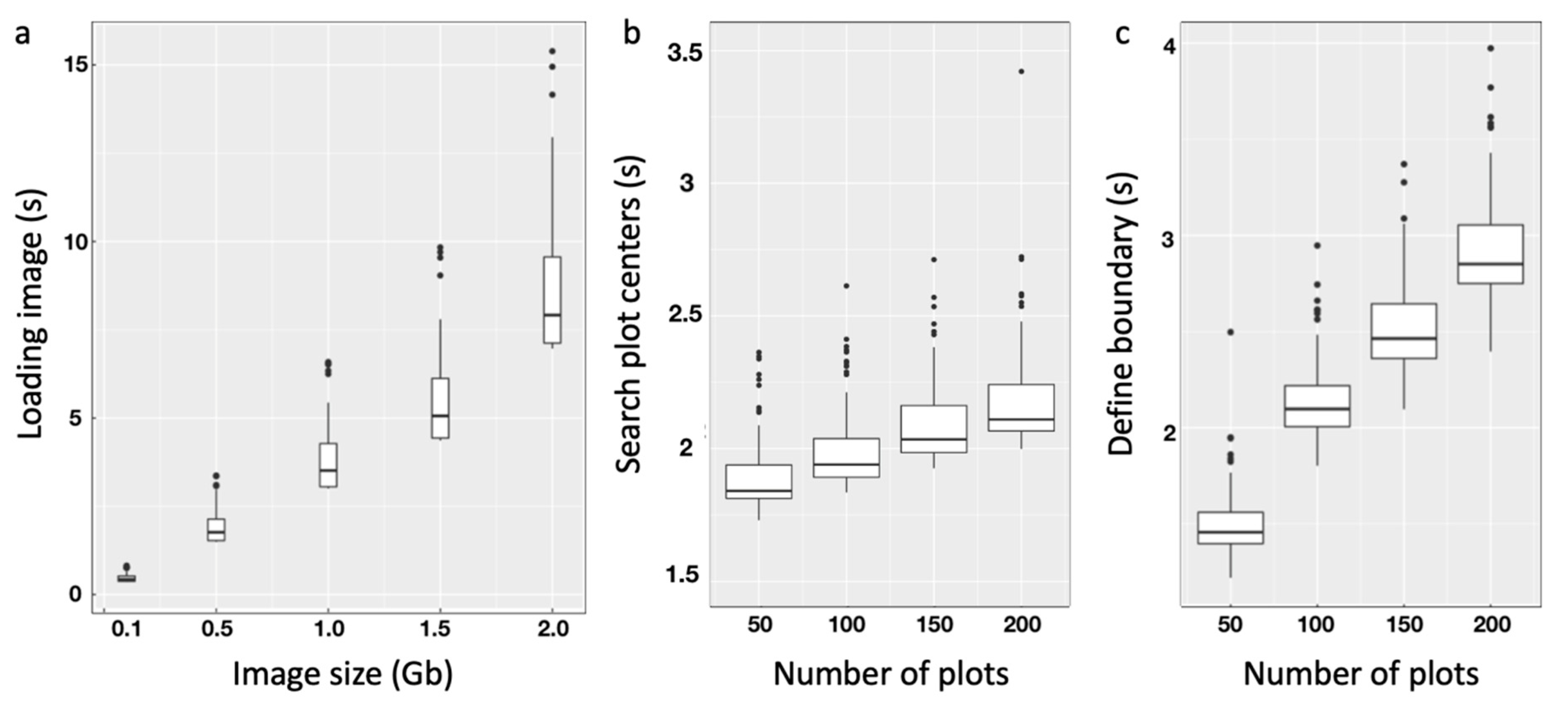
We evaluated the computation time relative to image file size and number of plots. The file size can significantly affect the image loading time. Furthermore, a large number of plots in an image can also increase the computing time, particularly during the search for plot centers and the boundary bargaining process. We modified the first orthomosaic into different circumstances to assess GRID’s performance relative to speed. The image was resized to 0.1 GB, 0.5 GB, 1 GB, 1.5 GB, and 2 GB, and the loading time was measured for each file size. We also cropped the image into smaller numbers of plots—50, 100, 150, and 200— and then evaluated how fast GRID performed plot searching and boundary bargaining. Each speed evaluation was conducted 100 times, reported as the mean and standard deviation, and visualized with a boxplot. The test environments were implemented on an Apple MacBook with Intel Core i9-8959HK CPU @ 2.9 GHz, 32 GB 2400 MHz DDR4 RAM, and Radeon Pro Vega 20 4GB GPU.

3. Results

3.1. Segmentation on a Variety of Plot Layouts

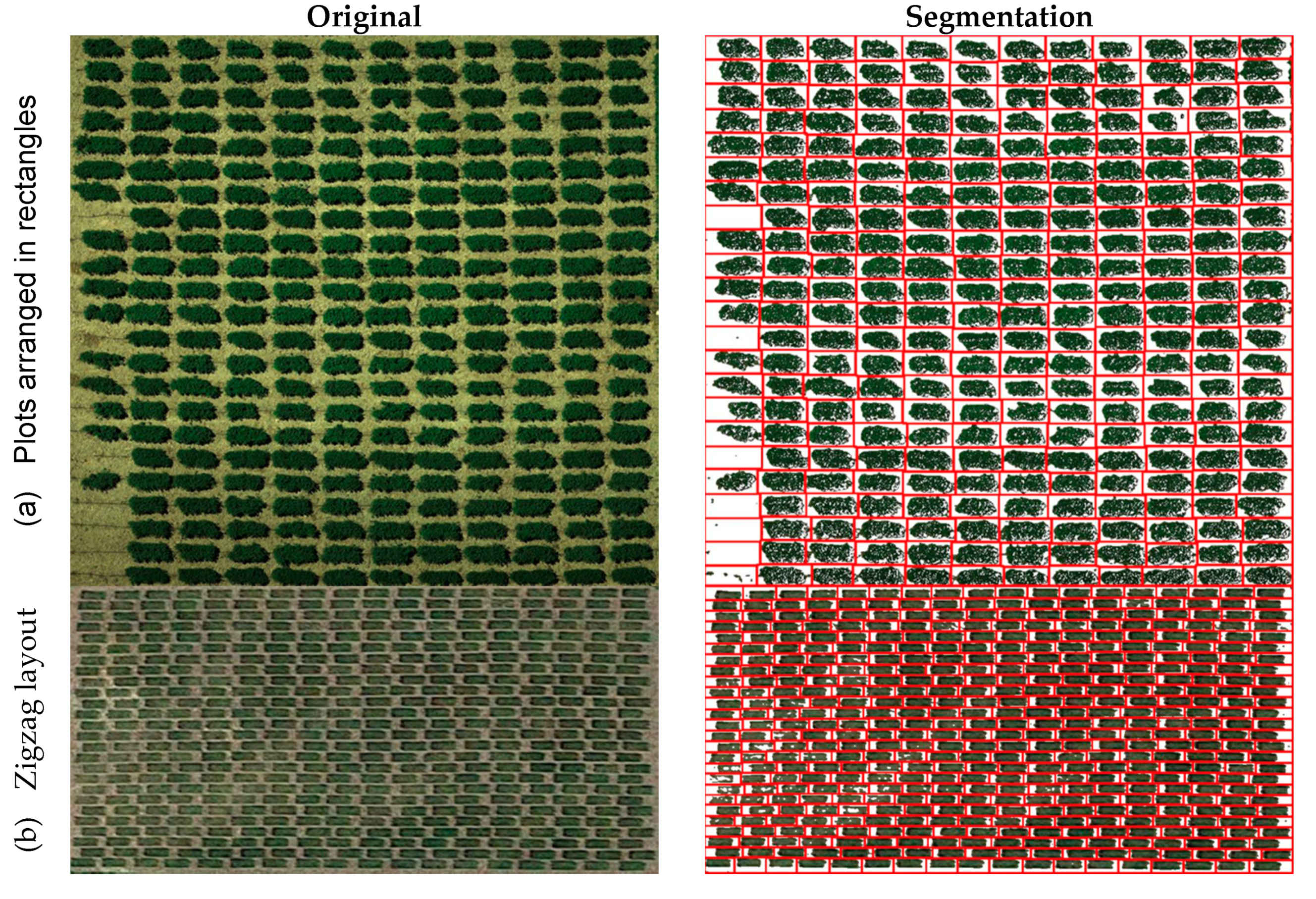
We tested GRID on a variety of plot layouts (Figure 5 and Figures S1–S3), including straight rows and columns, zigzag, rhombus, and multiple rows in a zigzag layout. An alfalfa field with plots in straight rows and columns was chosen to demonstrate the control of noise and shade (Figure 5a). Plots in the same row were connected by a visible drip irrigation pipe. GRID removed most pipes and replaced them with empty areas (white pixels), ensuring they would not be considered part of the segmented plots. The alfalfa field image also included plots that appeared to have connected leaf canopies, which present ambiguous areas for the segmentation. For instance, we observed that plots grown in the 5th row from the top, 2nd and 3rd columns from the left, were connected by their leaf canopies. With noise removal and clues from POI distribution, GRID recognized them as different plots and found a proper boundary to separate them. Within the final results, many white areas can be observed in each plot. Compared to adjacent pixels, these areas were mainly darker pixels, which GRID recognized as shade areas. These dark pixels are replaced with white pixels to achieve shade removal and prevent these non-vegetation pixels from causing information bias. GRID is also tolerant of missing plots. For example, about one-fourth of the plots in the left column of the alfalfa field were missing, but GRID still automatically recognized this column.

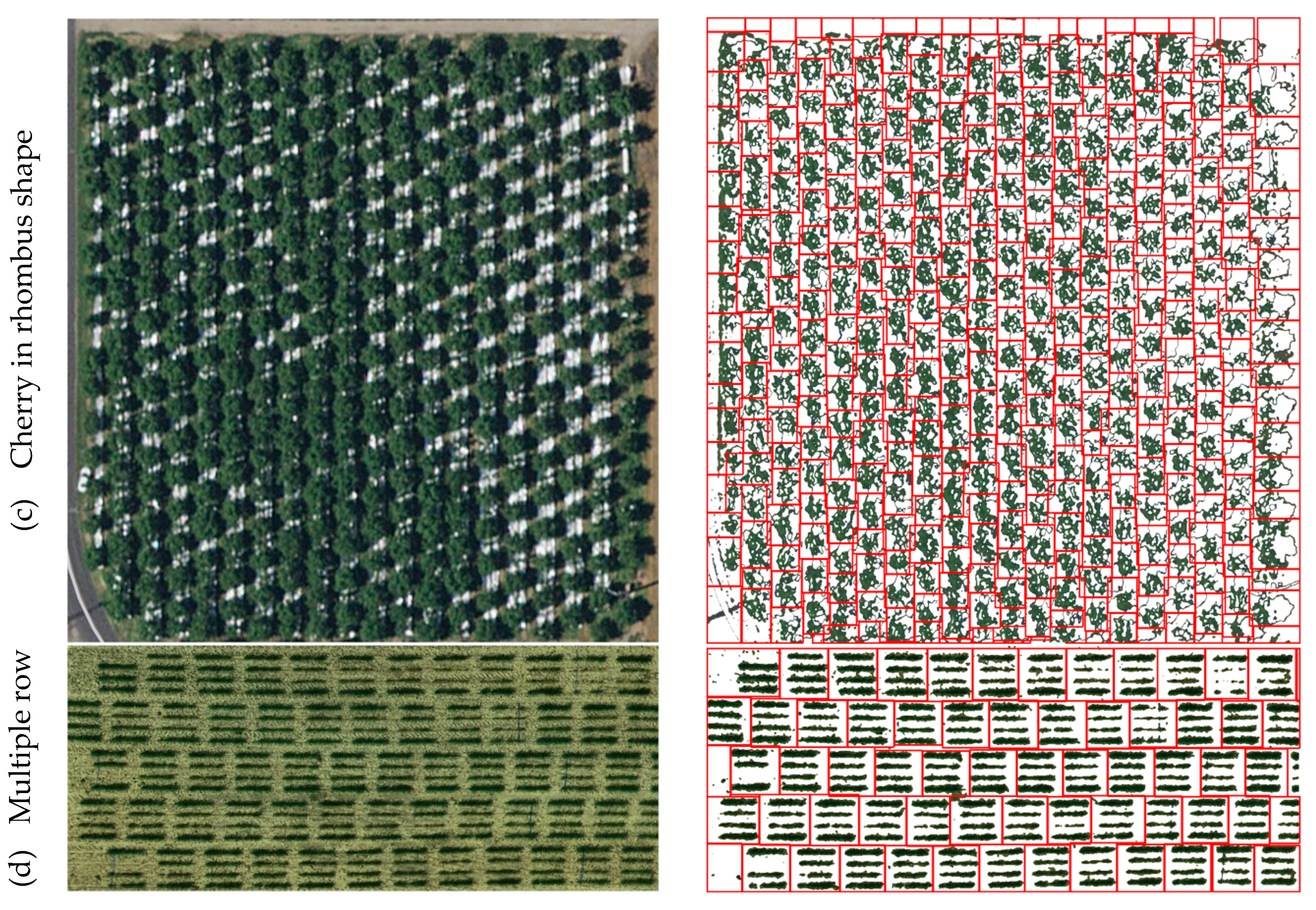
Two satellite images were chosen to demonstrate the tolerance of GRID on low resolution—one image of wheat with zigzag plots (Figure 5b) and one image of cherry trees arranged in a rhombus shape (Figure 5c). The wheat field is located on the Spillman Experimental Farm at Washington State University in Pullman, Washington (WA), U.S.A. Testing germplasms were continuously planted one after another in rows. Rows were separated by empty spaces. The individual plants adjacent to two germplasms were treated with herbicide for removal to ensure that all plots were the same size. Although the resolution was low, GRID clearly separated the plots. The cherry tree orchard is located in Grandview, WA, U.S.A. These trees varied in both shape and size. The image was taken when the sun cast a black shadow from each tree in the direction of the neighboring tree above and to the right. In addition, the soil at the base of the trees was covered with white plastic for weed control. GRID successfully removed both the shade and the background plastic.

Another wheat field image by drone (Figure 5d) was chosen to demonstrate the capability of GRID to process the difference between the visual appearance and actual plots. In this field, each test plot was arranged with four separate rows, which should be combined for analysis instead of segmenting each row as a single plot. Another challenge in this image is that the rows and columns of plots are not arranged in straight lines. By providing the number of plots in the field, GRID can still detect the proper layout even when plots are not arranged perpendicularly. In addition, some unusual objects existed within the plots. For example, one plot grown in the 1st row from the top and 2nd column from the right and one plot in the 3rd row from the top and 2nd column from the right have stripe-patterned objects across all four sub-row plants. By comparing the spectral information from the given image, GRID can recognize those objects as non-POI and remove them from the results. However, in this case, the contrast between POI and background was weak, so that these irrelevant objects were not completely removed. Similarly, in the alfalfa field example above, some drip irrigation pipes can still be observed after the segmentation. However, overall, plots were well segmented and are representative of their spectral variation.

3.2. Extraction of Plot Features

For all the POI of a plot, GRID calculates their average and standard deviation for all the channels of the input image. Six vegetation indices are also calculated pixel-wise, with their average and standard deviation as output for each plot. The six vegetation indices include the Normalized Difference Vegetation Index (NDVI) [18], Green Normalized Difference Vegetation Index (GNDVI) [19], Combination of Normalized Difference Vegetation Index (CNDVI) [20], Ratio Vegetation Index (RVI) [21], Green Ratio Vegetation Index (GRVI) [22], and Normalized Difference Greenness Vegetation Index (NDGVI) [23] (Table S1, Figure S4). For each segmented plot, GRID extracts both plot area and vegetation area in units of the number of pixels. Plot area includes the vegetation area and the areas of non-interest, such as soil background, shade, and weeds. The extracted information can serve as imagery features associated with plant growth and potential indicators of plant vigor.

3.3. Intermediate Images for Diagnosis and Futher Studies

Multiple intermediate images record the major processes of image analyses by GRID. These processes include pixel-wise cluster analysis, POI class selection, plot center location, and plot segmentation (Figure 5 and Figure 6). These images usually have much better resolution than the displays on the GRID interface. These intermediate images can be compared to the original image and used to evaluate whether the analysis was conducted appropriately. For example, users can verify if any clusters were missed as POI or any clusters were incorrectly classified as POI. The centers and boundaries on the original image provide a convenient way to assess the accuracy of the segmentation.

In addition, the segmented images contain more and potentially highly valuable information than what is reported by GRID as text files. For example, a single plot in a segmented image can exhibit visible characteristics that are biologically important. The plot length may relate to plant standing counts. The distribution of shade may be useful for evaluating canopy coverage, which is critical for weed control and water-use efficiency. To accommodate such a need for extracting additional image information, GRID outputs the segmented plots in numpy arrays and saves them as HDF5 files. The numpy arrays are commonly used for matrix computations, which can then be used for further image analyses, including their application as training and testing data for machine learning.

3.4. Computing Time

In the step of loading images, we observed a linear relationship between the file size and the median of the elapsed time from 100 iterations (Figure 7). For most cases, files smaller than 1 gigabyte can be loaded within 5 s, and a 2 gigabytes file takes less than 10 s to load in our testing environment. In terms of computing speed stability, which refers to the potential for differences in elapsed time from one iteration to another, loading a larger file may result in a greater variation in elapsed times. In addition, plot number is another factor that can limit computing speed. In the step of plot searching, we found that every extra 50 plots takes another 0.2 s to compute. With 200 plots, only 1 out of 100 iterations may take more than 3 s to finish the search. The boundary bargaining step takes a little more time than plot searching. On average, an image with 200 plots takes 2.8 s to finish the bargaining process, and 4 out of 100 iterations may take more than 3.5 s. Thus, we observed that the computation time for both crucial steps, plot searching and boundary bargaining, also increases linearly with the number of segmented plots.

4. Discussion

4.1. Advantages of Using GRID

GRID can be applied to a variety of plot layouts. These layouts include not only rows and columns arranged perpendicularly, but also rhombus patterns (i.e., rows and columns offset at 60-degree angles) and zigzag patterns (i.e., rows and columns are offset at angles less than 60 degrees). Two design features explain GRID’s wide adaptability relative to plot layout. First, GRID allows rows to intersect with columns at any angle, which leads to the more accurate placement of plot centers close to or at the actual center of the plots. Second, GRID’s segmentation process is tolerant of estimated plot centers that are less accurate, as long as the actual plot centers are within the POI of the plots. For example, the wheat plots in the satellite image were offset at a very narrow angle between the rows and columns. When GRID applied straight rows and columns at 90 degrees, some of the plots centers were placed at the center of plots, and some were placed at the end of plots. The bargaining process proceeded all the way to the other side of plots. As a result, GRID performed satisfactory segmentation for both types of plots, whether the plot center was located at the center or at the end of the plots (Figure 5b).

4.2. Operation Parameter File and Batch Processing

GRID stores operation parameters in a file named GRID.grid, which was designed for batch processing. However, conducting satisfactory analyses through batch segmentation remains challenging. In practical scenarios, users may have a series of images taken across different seasons. Parameters used in one image cannot be guaranteed to reproduce the same quality of outcomes when applied to another image taken in a different season. One reason for the different outcomes is that field management practices vary according to different crop growth stages. For example, herbicides are rarely used in the early growing stage, so both weeds and seedlings will look similar in terms of their color when observed in an image. This fact may cause difficulties for our algorithm when it attempts to differentiate two objects based solely on imagery channels. The current workaround is that instead of detecting POI via pixel-based clustering, GRID allows users to manually specify plot locations and sizes. Since we expect plots to remain in the same locations over time, anchoring their coordinates and expected sizes ensures better plot segmentation compared with spectral signals, which can change dramatically over time.

4.3. GRID-Based Vegetation Indices Output Versus User-Defined Output

GRID outputs the plot averages and standard deviations of six vegetation indices that are calculated pixel-wise from the channels of the original images. However, other indices may be of particular interest to specific researchers. Some researchers may even be interested in defining their own indices. With the output of plot averages and standard deviations, GRID users can derive other vegetation indices of interest. Calculations are slightly different for indices derived by the users compared to the indices of GRID’s output. For GRID’s output, the indices are calculated pixel-wise first, and then the averages and standard deviation are calculated. For the indices derived by users, the averages of the image channels must be used to calculate plot averages, which can offer relatively good approximations. However, the derivation of the standard deviation within a plot for user-defined indices is not straight forward because pixel-wise data are unavailable.

4.4. Boundary Bargaining Between Adjacent Neighbors

Although each plot has eight potential adjacent neighbors, boundary bargaining is only conducted with the neighbors in the same rows and columns, having no boundary overlap between them. That is, no bargaining occurs between the neighbors on the diagonals and not in the same rows or columns. As a result, a plot has the potential to share the same area with neighbors on the diagonals, which means that the total plot area may exceed the total image area. For plots with layouts in straight rows and columns, this problem is negligible. However, for other plot layouts, this problem could be severe.

4.5. Limitations

Currently, GRID only provides two options, either 0 or 90 degrees, when choosing rows or columns as the major axis of the field plot layout. When rows are chosen as the major axis, the columns are defined as the minor axis, and vice versa. In contrast, the minor axis can be optimized or adjusted to any angle degree that matches the layout. This approach works for images with either rows or columns that align with either the vertical or horizontal direction of the image. For images that do not have such properties, users can crop the images to satisfy the requirement. In such cases, the area of interest will be partially removed if near image edges, especially if near the corners.

GRID assumes the first three channels are the visible channels (RGB) and uses their average to control shade and noise. Thus, this assumption is invalidated for some multispectral images that capture other wavelengths. This assumption can also cause problems for calculating vegetation indices. GRID does not allow users the flexibility to define the channels and derive the vegetation indices accordingly. Users must arrange the channels based on the assumption of GRID. Otherwise, the adjustments on shade and noise should be conducted with caution. The output of vegetation indices should be interpreted accordingly or calculated from the values of channels.

Certain situations make it difficult for GRID to select POI or to segment. One situation that affects the selection of POI is a field filled with weeds that look very similar to the crop of interest. In many cases, weeds are distinguishable from crops so that weeds can be assigned to a cluster different from crops. Consequently, weeds are considered as background and will not affect layout detection and boundary determination. However, if weeds are nearly identical to the vegetation of interest for all channels, including RGB and other multispectral channels, GRID is unable to accurately select POI. Another situation that affects the segmentation is a field that contains a significant number of missing plots or a field layout of plots that is barely visible to human eyes. In these cases, GRID will have problems detecting the layouts automatically. Users must manually conduct the segmentation by defining the number of rows and columns.

GRID uses a pixel as the unit in its outputs, including the area of vegetation. Results from different images are comparable only if they have the same resolution. To compare images with different resolutions, users have to set reference objects in each image and transform the original GRID outputs accordingly.

5. Conclusions

GRID is a user-friendly tool that automatically produces segmentation for images with minimal human involvement. GRID is capable of detecting different types of field layouts, including plots arranged in grid or rhombus patterns. As a result, GRID produces more precise outcomes compared to other software programs that can only define AOI by drawing polygons. In terms of computing speed, GRID can handle data larger than 1 gigabyte and more than 100 test plots within one minute. The computing time is linear to the file size and plot number. This feature allows users to scale up their analyses to larger areas of field plots. Moreover, GRID is implemented with an interactive GUI. With a real-time preview panel in the interface, users are expected to experience a smooth learning curve using GRID. Since any change made in the software options during the plot segmentation process can be previewed before exporting the final results, users can compare the outcomes from different configurations intuitively. GRID is expected to be an effective tool for extracting field plot features, which can then be used directly for high-throughput phenotyping and further analyses in agricultural research.

References

- Li, L.; Zhang, Q.; Huang, D. A Review of Imaging Techniques for Plant Phenotyping. Sensors 2014, 14, 20078–20111. [Google Scholar] [CrossRef] [PubMed]
- QGIS Development Team. QGIS Geographic Information System; Open Source Geospatial Foundation: Beaverton, OR, USA, 2009. [Google Scholar]
- Salvacion, A.R. Terrain characterization of small island using publicly available data and open-source software: A case study of Marinduque, Philippines. Model. Earth Syst. Environ. 2016, 2, 31. [Google Scholar] [CrossRef] [Green Version]
- Maliqi, E.; Penev, P.; Kelmendi, F. Creating and analysing the Digital Terrain Model of the Slivovo area using QGIS software. Geodesy Cartogr. 2017, 43, 111–117. [Google Scholar] [CrossRef] [Green Version]
- Brown, J.C.; Kastens, J.H.; Coutinho, A.C.; de Castro Victoria, D.; Bishop, C.R. Classifying multiyear agricultural land use data from Mato Grosso using time-series MODIS vegetation index data. Remote Sens. Environ. 2013, 130, 39–50. [Google Scholar] [CrossRef] [Green Version]
- Groenendyk, D.G.; Ferré, T.P.A.; Thorp, K.R.; Rice, A.K. Hydrologic-Process-Based Soil Texture Classifications for Improved Visualization of Landscape Function. PLoS ONE 2015, 10, e0131299. [Google Scholar] [CrossRef] [Green Version]
- Nga, D.V.; See, O.H.; Quang, D.N.; Xuen, C.Y.; Chee, L.L. Visualization Techniques in Smart Grid. Smart Grid Renew. Energy 2012, 3, 175. [Google Scholar] [CrossRef] [Green Version]
- Hearst, A.; Rainey, K. Progeny. Available online: https://www.progenydrone.com (accessed on 20 October 2019).
- Tresch, L.; Mu, Y.; Itoh, A.; Kaga, A.; Taguchi, K.; Hirafuji, M.; Ninomiya, S.; Guo, W. Easy MPE: Extraction of Quality Microplot Images for UAV-Based High-Throughput Field Phenotyping. Plant Phenomics 2019, 2019, 1–9. [Google Scholar] [CrossRef] [Green Version]
- Khan, Z.; Miklavcic, S.J. An Automatic Field Plot Extraction Method from Aerial Orthomosaic Images. Front. Plant Sci. 2019, 10, 683. [Google Scholar] [CrossRef] [PubMed]
- Kennedy, J.; Eberhart, R. Particle swarm optimization. In Proceedings of the ICNN’95—International Conference on Neural Networks, Perth, WA, Australia, 27 November–1 December 1995; Volume 4, pp. 1942–1948. [Google Scholar]
- Arganda-Carreras, I.; Kaynig, V.; Rueden, C.; Eliceiri, K.W.; Schindelin, J.; Cardona, A.; Sebastian Seung, H. Trainable Weka Segmentation: A machine learning tool for microscopy pixel classification. Bioinformatics 2017, 33, 2424–2426. [Google Scholar] [CrossRef] [PubMed]
- Summerfield, M. Rapid GUI Programming with Python and Qt: The Definitive Guide to PyQt Programming; Pearson Education: London, UK, 2008. [Google Scholar]
- Swan, G. Rasterio: Geospatial Raster I/O for Python Programmers; Mapbox: Washington, DC, USA, 2013. [Google Scholar]
- van der Walt, S.; Colbert, S.C.; Varoquaux, G. The NumPy Array: A Structure for Efficient Numerical Computation. Comput. Sci. Eng. 2011, 13, 22–30. [Google Scholar] [CrossRef] [Green Version]
- Bradski, G. The OpenCV Library. Dr. Dobb’s Journal of Software Tools. 2000. Available online: https://opencv.org/ (accessed on 2 April 2020).
- Virtanen, P.; Gommers, R.; Oliphant, T.E.; Haberland, M.; Reddy, T.; Cournapeau, D.; Burovski, E.; Peterson, P.; Weckesser, W.; Bright, J.; et al. SciPy 1.0: Fundamental Algorithms for Scientific Computing in Python. Nat. Methods 2020, 17, 261–272. [Google Scholar] [CrossRef] [PubMed] [Green Version]
- Rouse, W.; Haas, R.H. Monitoring Vegetation Systems in the Great Plains with Erts. NASA Spec. Publ. 1974, 351, 309. [Google Scholar]
- Gitelson, A.A.; Kaufman, Y.J.; Merzlyak, M.N. Use of a green channel in remote sensing of global vegetation from EOS-MODIS. Remote Sens. Environ. 1996, 58, 289–298. [Google Scholar] [CrossRef]
- Sun, H.; Li, M.; Zheng, L.; Zhang, Y.; Yang, W. Evaluation of maize growth by ground based multi-spectral image. In Proceedings of the 2011 IEEE/SICE International Symposium on System Integration (SII), Kyoto, Japan, 20–22 December 2011; pp. 207–211. [Google Scholar]
- Jordan, C.F. Derivation of Leaf-Area Index from Quality of Light on the Forest Floor. Ecology 1969, 50, 663–666. [Google Scholar] [CrossRef]
- Sripada, R.P.; Heiniger, R.W.; White, J.G.; Weisz, R. Aerial Color Infrared Photography for Determining Late-Season Nitrogen Requirements in Corn. Agron. J. 2005, 97, 1443–1451. [Google Scholar] [CrossRef]
- Baret, F.; Guyot, G. Potentials and limits of vegetation indices for LAI and APAR assessment. Remote Sens. Environ. 1991, 35, 161–173. [Google Scholar] [CrossRef]
Figure 1.
Workflow of GReenfield Image Decoder (GRID). GRID takes an image (a) and an optional field layout text file (b) as input data. Users can either use the original image or a cropped image (c). The image is classified pixel-wise (d), and the clusters of interest can be selected to define pixels of interest (POI) (e). The POI from the selected clusters are displayed as yellow, and all non-POI are displayed as black. POI can be fine-tuned by removing shade (f) and noise (g). The plot centers (h) and boundaries (i) are automatically created and displayed as the red crosses and boxes, respectively. GRID output includes the text file (j) and images corresponding to (d,e,i). GRID not only processes grid patterns in rectangle shapes, but also other patterns, such as rhombus shapes (k).
Figure 2.
Convolution operation for noise reduction. A binary image (B) is smoothed by the Gaussian kernel (ω). The binary image contains two pixels of 0s (open cells) that are surrounded by 1s (shaded cells) and considered noise. The convolution operation generates a matrix with the two noise cells filled by values above the Gaussian threshold (0.5). The transformed binary image displays the removed noise.
Figure 3.
Automatic detection of plot layout through image rotation. The input image has a layout arranged in a rhombus shape (a). The rotation of the POI image is demonstrated at 15-degree intervals (b). Vertical-scan signal f(x) is an average value at the position x of the POI image, where x is the horizontal position of the POI image (c). Frequency domains are computed via Fourier transformation, where is the signal frequency over f(x) (d). is used to determine the optimal rotation of the field image. When the correct rotation matches Fourier transformation, the frequency domain contains a single peak with a high POI density relative to other rotations. This example demonstrates that valid rotations (45° and 90°) have repeating vertical POI density patterns that, when Fourier transformed, result in a frequency domain that can determine the optimal rotation. Red stars shown in the two optimal rotations represent the plot centroids in (c) and the single peaks of frequency domain (d).
Figure 4.
Boundary bargaining between adjacent plots. The bargaining between two plots starts at their center points in either column or row directions (a, left). The final boundaries (a, right) are determined by the movement of bargaining bars. A bargaining bar moves away from its center if it has more power than its opponent. The power of a bargaining bar is defined by its proportion of pixels of interest (POI, red area on the bar itself) over the total pixels (red + blue on the bar) adjusted by a penalty. The penalty is a bargaining bar’s distance to its plot center (lower case red d) divided by the distance between the centers of the two plots (upper case red D), multiplied by a weight (default of 0.2). The right plot has more power than the left plot and reaches its left edge first (b). When left and right plots do not have POI intersecting their bargaining bars, both bars move forward (c). After the left plot finds its separated POI, it gains power and moves to the right edge (d). At the end of the bargaining process, both plots run out of POI and the bars move simultaneously to complete the connection and form the boundary (e).
Figure 5.
Segmentation of images with different plot layout patterns and resolutions. The patterns include perpendicular layout of alfalfa (a), zigzag-like layout of wheat (b), rhombus shape of cherry tree orchard (c), and multiple rows within plots of pea field (d). The alfalfa and pea field drone images were provided by Zhou Tang and Samuel Revolinski. The other two are Google satellites images for wheat on Spillman Agronomy Farm at Washington State University (46°41′50.8″N 117°07′29.1″W) and for cherry trees in Grandview, Washington (46.230664, 119.904291). The left panel displays the raw images and the right panel demonstrates the extracted pixels of interest with plots defined by the red boxes.
Figure 6.
Multiple intermediate images of segmentation. GRID saves multiple intermediate images for documentation, diagnosis, and further image analyses. These intermediate images demonstrate the pixel-wise cluster analysis (a), the plot centers on selected pixels of interest (b), and the raw image (c). The plot boundaries are displayed on both selected pixels of interest (d) and the raw image (e). The pixels of interest are displayed for the raw image with pixels of non-interest displayed as white background (f), which are also saved as HDF5 for each of segmented plots as numpy arrays. The raw image was taken by drone on the alfalfa field in Figure 5.
Figure 7.
Linear computing complexity over file size and the number of plots. The total running times in seconds (s) were divided into times (s) for loading images (a), searching plot centers (b), and defining boundaries (c). The image loading time is linear to the image size. The running times for both searching plot centers and defining boundaries through bargaining between adjacent plots are linear to number of plots.
© 2020 by the authors. Licensee MDPI, Basel, Switzerland. This article is an open access article distributed under the terms and conditions of the Creative Commons Attribution (CC BY) license (http://creativecommons.org/licenses/by/4.0/).
Share and Cite
MDPI and ACS Style
Chen, C.J.; Zhang, Z. GRID: A Python Package for Field Plot Phenotyping Using Aerial Images. Remote Sens. 2020, 12, 1697. https://0-doi-org.brum.beds.ac.uk/10.3390/rs12111697
AMA Style
Chen CJ, Zhang Z. GRID: A Python Package for Field Plot Phenotyping Using Aerial Images. Remote Sensing. 2020; 12(11):1697. https://0-doi-org.brum.beds.ac.uk/10.3390/rs12111697
Chicago/Turabian StyleChen, Chunpeng James, and Zhiwu Zhang. 2020. "GRID: A Python Package for Field Plot Phenotyping Using Aerial Images" Remote Sensing 12, no. 11: 1697. https://0-doi-org.brum.beds.ac.uk/10.3390/rs12111697
Note that from the first issue of 2016, this journal uses article numbers instead of page numbers. See further details here.