Review: Deep Learning on 3D Point Clouds
by
 , ,
, ,
Saifullahi Aminu Bello
1,2 ,
,
Shangshu Yu
1,
Cheng Wang
1,*,
Jibril Muhmmad Adam
1 and
Jonathan Li
1,3 1
Fujian Key Laboratory of Sensing and Computing for Smart City, School of Informatics, Xiamen University, 422 Siming South Road, Xiamen 361005, China
2
Department of Computer Science, Kano University of Science and Technology, Wudil, P.M.B 3244 Kano State, Nigeria
3
Department of Geography and Environmental Management, University of Waterloo, 200 University Avenue, Waterloo, ON N2L 3G1, Canada
*
Author to whom correspondence should be addressed.
Remote Sens. 2020, 12(11), 1729; https://0-doi-org.brum.beds.ac.uk/10.3390/rs12111729
Submission received: 21 April 2020
/
Revised: 20 May 2020
/
Accepted: 20 May 2020
/
Published: 28 May 2020
(This article belongs to the Special Issue GeoAI: Integration of Artificial Intelligence, Machine Learning and Deep Learning with Remote Sensing)
Abstract
:A point cloud is a set of points defined in a 3D metric space. Point clouds have become one of the most significant data formats for 3D representation and are gaining increased popularity as a result of the increased availability of acquisition devices, as well as seeing increased application in areas such as robotics, autonomous driving, and augmented and virtual reality. Deep learning is now the most powerful tool for data processing in computer vision and is becoming the most preferred technique for tasks such as classification, segmentation, and detection. While deep learning techniques are mainly applied to data with a structured grid, the point cloud, on the other hand, is unstructured. The unstructuredness of point clouds makes the use of deep learning for its direct processing very challenging. This paper contains a review of the recent state-of-the-art deep learning techniques, mainly focusing on raw point cloud data. The initial work on deep learning directly with raw point cloud data did not model local regions; therefore, subsequent approaches model local regions through sampling and grouping. More recently, several approaches have been proposed that not only model the local regions but also explore the correlation between points in the local regions. From the survey, we conclude that approaches that model local regions and take into account the correlation between points in the local regions perform better. Contrary to existing reviews, this paper provides a general structure for learning with raw point clouds, and various methods were compared based on the general structure. This work also introduces the popular 3D point cloud benchmark datasets and discusses the application of deep learning in popular 3D vision tasks, including classification, segmentation, and detection.
1. Introduction
We live in a three-dimensional world; however, since the invention of the camera, visual information of the 3D world has been projected onto 2D images. Two-dimensional images, however, lose depth information and relative positions between two or more objects in the real world. These factors make 2D images less suitable for applications that require depth and positioning information such as robotics, autonomous driving, virtual reality, and augmented reality, among others [1,2,3]. To capture the 3D world with depth information, the early convention was to use stereo vision, where two or more calibrated digital cameras are used to extract 3D information [4,5]. A point cloud is a data structure that is often used to represent 3D geometry, as the immediate representation of the extracted 3D information from stereo vision cameras [6,7] as well as of the depth map produced by RGB-D. Recently, 3D point cloud data have become popular as a result of the increasing availability of sensing devices, especially light detection and ranging (LiDAR)-based devices such as Tele-15 [8], Leica BLK360 [9], Kinect V2 [10], etc., and, more recently, mobile phones with a time of flight (tof) depth camera. These sensing devices allow the easy acquisition of the 3D world in 3D point clouds.
A point cloud is simply a set of data points in space. The point cloud of a scene is the set of 3D points around the surfaces of the objects in the scene. In its simplest form, 3D point cloud data are represented by the XYZ coordinates of the points, or these may include additional features such as surface normals and RGB values. Point cloud data represent a very convenient format for representing the 3D world. Point clouds are commonly used as a data format in several disciplines such as geomatics/surveying (mobile mapping); architecture, engineering, and construction (AEC); and Building Information Modelling (BIM) [11,12,13]. Point clouds have a range of applications in different areas such as robotics [14], autonomous driving [15], augmented and virtual reality [16], manufacturing and building rendering [17], etc.
In the past, the processing of point clouds for visual intelligence has been based on handcrafted features [18,19,20,21,22,23]. A review of handcrafted-based feature learning techniques is conducted in [24]. The handcrafted features do not require large training data and have been seldom used due to insufficient point cloud data; furthermore, deep learning was not popular. However, with the increasing availability of acquisition devices, point cloud data are now readily available, making the use of deep learning for its processing feasible.
Deep learning is a machine learning approach based on artificial neural networks designed to mimic the human brain [25]. Deep learning models are used to learn feature representations of data through multiple processing layers that learn multiple levels of abstraction [26]. Deep learning models are used in several areas, including computer vision, speech recognition, natural language processing, etc. They have achieved state-of-the-art results comparable to—and in some instances surpassing—human expert performance [27,28,29].
In the computer vision field, deep learning has achieved notable success with 2D data [27,30,31,32,33]. However, the application of deep learning on 3D point clouds is not easy due to the inherent nature of the point clouds. In this paper, the challenges of using point clouds for deep learning are presented. This paper reviews the early approaches devised to overcome these challenges, and the recent state-of-the-art approaches that directly operate on the point clouds, focusing more on the latter. This paper is intended to serve as a guide to new researchers in the field of deep learning with point clouds as it presents the recent state-of-the-art approaches of deep learning with point cloud data. In contrast to existing reviews [34,35,36], this paper’s focus is mainly on point cloud data; it gives a general structure for learning with raw point clouds, and various methods are compared based on the general structure. Popular point cloud benchmarked datasets are also introduced and summarized in tabular form for easy analysis.
The rest of the paper is organized as follows: Section 2 discusses the methodology used. Section 3 discusses the challenges of point clouds which make the application of deep learning more difficult. Section 4 reviews the methods to overcoming these challenges by converting the point clouds into a structured grid. Section 5 contains in-depth information regarding the various deep learning methods that process point clouds directly. In Section 6, 3D point clouds benchmark datasets are presented. The application of the various approaches in the 3D vision tasks is discussed in Section 7. The summary and conclusion of the paper are given in Section 8.
2. Methodology
Articles reviewed in this paper were all published between 2015 to 2020. The article is mainly focused on point cloud data; however, it includes a brief review of other approaches based on structured 3D data. The article includes the first works that use deep learning on voxel-based and multiview 3D representation, which were published in 2015 and 2016, respectively. It also includes a few highly cited works on the two representations.
Deep learning with raw point clouds was pioneered by PointNet, published in 2017. The works reviewed in this category were published from 2017 to 2020. We have mainly searched for the relevant papers using the major conference repositories such as Conference on Computer Vision and Pattern Recognition (CVPR), International Conference on Computer Vision (ICCV), European Conference on Computer Vision (ECCV), Association for the Advancement of Artificial Intelligence (AAAI) Conference, International Conference on Learning Representations (ICLR) as well as Google Scholar. Many benchmarked datasets have an online leaderboard; we also consider leading works from these leaderboards.
The datasets selected in this paper were all published after 2010, and they mainly referenced common tasks in computer vision. The data are all tagged with ground truth (GT) labels. Tabular details were provided for the easy understanding of the datasets.
3. Challenges of Deep Learning with Point Clouds
Applying deep learning to 3D point cloud data has many challenges. These challenges include occlusion, which is caused by cluttered scenes or blindsides; noise/outliers, which are unintended points; and point misalignment, etc. [37,38]. However, the most significant challenges regarding the application of deep learning to point clouds can be categorized as follows:
Irregularity: Point cloud data are irregular, meaning that the points are not evenly sampled across the different regions of an object/scene, so some regions could have dense points while others have sparse points [39]. These can be seen in Figure 2a. Irregularity can be attenuated by sub sampling techniques, but cannot be completely eliminated [40].
Unstructured: Point cloud data are not placed on a regular grid [41]. Each point is scanned independently, and its distance to neighboring points is not always fixed. In contrast, pixels in images are represented on a two-dimensional grid, and the spacing between two adjacent pixels is always fixed.
Unorderdness: A point cloud of a scene is the set of points (usually represented by XYZ) obtained around the objects in the scene, and these are usually stored as a list in a file. As a set, the order in which the points are stored does not change the scene represented; therefore, it is invariant to permutation [42]. For illustration purposes, the unordered nature of point sets is shown in Figure 2c.
These properties of point clouds are very challenging for deep learning, especially convolutional neural networks (CNN). This is because CNNs are based on convolution operation, which is performed on data that are ordered, regular, and on a structured grid. Early approaches overcome these challenges by converting the point clouds into a structured grid format, as shown in Section 4. However, researchers have recently been developing approaches that directly use the power of deep learning for the raw point cloud, without the need for conversion to a structured grid; see Section 5.
4. Structured Grid-Based Learning
Deep learning, specifically the convolutional neural network (CNN), is successful because of the convolutional layer. The convolutional layer uses gradient descent to determine the filters (also referred to as kernels) for feature detection using the convolution operation. The convolution layer is used for feature learning, replacing the need for handcrafted features. Figure 3 shows a typical convolution operation on a 2D grid using a 3 × 3 filter. The convolution operation requires a structured grid. Point cloud data are unstructured, and this is a challenge for deep learning. To overcome this challenge, many approaches convert the point cloud data into a structured form. These approaches can be broadly divided into two categories: voxel-based and multi-view-based. This section reviews some of the state-of-the-art methods in both voxel-based and multi-view-based categories, as well as their advantages and drawbacks.
4.1. Voxel-Based Approach
The convolution operation for 2D images uses a 2D filter of size to convolve a 2D input, represented as matrix of size with and . Voxel-based methods [43,44,45,46,47] use a similar approach by converting the point clouds into a 3D voxel structure of size and convolving it with 3D kernels of size with , respectively. Basically, two important operations take place in this method: offline (preprocessing) and online (learning). The offline method converts the point clouds into fixed-size voxels, as shown in Figure 4. Binary voxels [48] are often used to represent the voxels. In NormalNet [46], a normal vector is added to each voxel to improve discrimination capability.
The online operation is the learning stage. In this stage, the deep convolutional neural network is designed, usually using a various number of 3D convolutional, pooling, and fully connected layers.
In 3D ShapeNets [48], 3D shapes are represented as a probability distribution of binary variables on a 3D voxel grid; this technique was the first to use 3D Deep Convolutional Neural Networks. The inputs to the network—point clouds, computer-aided design (CAD) models, or RGB-D images—are converted into a 3D binary voxel grid and are processed using a convolutional deep belief network [49]. A three-dimensional CNN is used for landing zone detection for unmanned rotorcraft in [43]. LiDAR from the rotorcraft is used to obtain point clouds of the landing site, which are then voxelized into 3D volumes, and a 3D CNN binary classifier is applied to classify the landing site as safe or otherwise. In VoxNet [44], a 3D convolutional neural network for object recognition is proposed. As with 3D ShapeNets [48], the input to VoxNet is converted into a 3D binary occupancy grid before applying 3D convolution operations to generate a feature vector which is passed through fully connected layers to obtain class scores. Two voxel-based models were proposed by Qi et al. [45]: the first model addressed overfitting using auxiliary training tasks to predict objects from partial subvolumes, while the second model mimicked multi-view CNNs by convolving the 3D shapes with an anisotropic probing kernel.
Although voxel-based methods have shown good performance, they suffer from high memory consumption due to the sparsity of the voxels, as shown in Figure 4. The voxel sparsity results in wasted computation when convolving over the non-occupied regions. The memory consumption also limits the voxel resolution, usually to between 32 cubes and 64 cubes. These drawbacks are also in addition to the artifacts introduced by the voxelization operation.
4.2. Multi-View-Based Approach
Multi-view-based methods [45,52,53,54,55,56,57,58] take advantage of the benefits of the already matured 2D CNNs and apply them into three dimensions. Because images are actual representations of the 3D world squashed onto a 2D grid by a camera, methods in this category follow this technique by converting point cloud data into a collection of 2D images and applying existing 2D CNN techniques to it; see Figure 5. Compared to their volumetric-based counterparts, multi-view based methods have better performance, as the multi-view images contain texture information, unlike 3D voxels, even though, the latter contain depth information.
MultiviewCNN [52] was the first approach in this direction. The proposed network bypassed the need for 3D descriptors for recognition and achieved state-of-the-art accuracy. Leng et al. [53] proposed a stacked local convolutional autoencoder (SLCAE) for 3D object retrieval. Multi-resolution filtering, which captures information at multiple scales, was introduced by Qi et al. [45]; besides, the authors used data augmentation for better generalization. RotationNet [58] uses rotation to select the best viewpoint that maximizes the class likelihood; it leads the Modelnet40 [48] leaderboard at the time of this review.
Multi-view based networks have better performance than voxel-based methods; this is because (1) they use 2D techniques which have already been well researched and (2) they can contain richer information as they do not have the quantization artifacts of voxelization.
4.3. Higher-Dimensional Lattices
There are other methods for point cloud processing using deep learning that convert the point clouds into a higher-dimensional regular lattice. SplatNet [59] processes point clouds directly; however, the primary feature learning operation occurs at the bilateral convolutional layer (BCL). The BCL layer converts the features of unordered points into a six-dimensional (6D) permutohedral lattice and convolves it with a kernel of a similar lattice. SFCNN [60] uses a fractalized regular icosahedral lattice to map points onto a discretized sphere and define a multi-scale convolution operation on the regular spherical lattice. Compared to voxel-based and multi-view approaches, [59,60] have better performance in terms of segmentation with SplatNet, achieving state-of-the-art accuracy on semantic segmentation. They are also better than the voxel-based approach in terms of classification.
5. Deep Learning Directly with a Raw Point Cloud
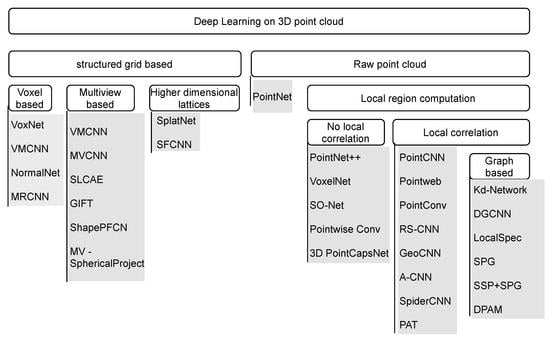
Deep learning with raw point clouds has received increased attention since PointNet [42] was released in 2017. Many state-of-the-art methods have been developed since then; these techniques process point clouds directly despite the challenges listed in Section 3. In this section, the state-of-the-art techniques that work in this direction are reviewed. The development of this began with PointNet, which is the bedrock for most methods. Other methods improved on PointNet by modeling local region structures.
5.1. PointNet
Convolutional neural networks use convolutional layers to learn hierarchical feature representations as the network deepens [27]. Convolutional layers use a convolution that requires a structured grid, which is lacking in point cloud data. PointNet [42] was the first method to apply deep learning to an unstructured point cloud, and it formed the basis from which most other techniques were developed.
The architecture of PointNet is shown in Figure 6. The input to PointNet is a raw point cloud , where N represents the number of points in the point cloud and D the dimension. Usually, , representing the XYZ values of each point; however, additional features can be used. Because points are unordered, PointNet is built on two basic functions: multilayer perceptron (MLP), with learnable parameters, and a maxpooling function. The MLPs are feature transformations that transform the feature dimension of the points from a to dimensional space, and their parameters are shared by all the points in each layer. To obtain a global feature, the maxpooling function is used as a symmetric function. A symmetric function is a function whose output is the same irrespective of the input order. The maxpooling produces one global 1024-dimensional feature vector. The feature vector represents the feature descriptor of the input, which can be used for recognition and segmentation tasks.
PointNet achieved state-of-the-art performance on several benchmark datasets. The design of PointNet, however, does not consider the local dependency among points; thus, it does not capture the local structure. The global maxpooling applied selects the feature vector with a “winner-takes-all” [61] principle, making it very susceptible to a targeted adversarial attack, as demonstrated by Xiang et al. [62]. After PointNet, many approaches were proposed to capture local structures.
5.2. Approaches with Local Structure Computation
Many state-of-the-art approaches were developed after PointNet to capture local structures. These techniques capture the local structure hierarchically in a similar fashion to grid convolution, with each hierarchy encoding a richer representation.
Basically, due to the inherent unstructuredness of point clouds, local structure modeling is based on three basic operations: sampling, grouping, and a mapping function. The mapping function is usually approximated by a multilayer perceptron (MLP) which maps the features of the nearest neighbor points into a feature representation that encodes higher-level information; see Figure 7. These operations are briefly explained before reviewing the various approaches.
Sampling is employed to reduce the resolution of points across layers in the same way that the convolution operation reduces the resolution of feature maps via convolutional and pooling layers. Given a point cloud of N points, the sampling reduces it to M points , where . The subsampled M points, also referred to as representative points or centroids, are used to represent the local region from which they were sampled. Two approaches are popular for subsampling: (1) random point sampling, where each of the N points is equally likely to be sampled; and (2) farthest point sampling (FPS), where the M points are sampled such that each sampled point is the most distant point from the rest of the points. Other sampling methods include uniform sampling and Gumbel subset sampling [63].
As regards the grouping operation, as the representative points are sampled, the k-nearest neighbor (kNN) algorithm is used to select the nearest neighbor points to the representative points to group them into a local patch; see Figure 8. The points in a local patch are used to compute the local feature representation of the neighborhood. In grid convolution, the receptive field shows the pixels on the feature map under a kernel. The kNN is either used directly, where k nearest points to a centroid are sampled, or a ball query is used. With ball query, points are selected only when they are within a certain radius distance to the centroid points.
Regarding the non-linear mapping function, once the nearest points to each representative point are obtained, the next step is to map them into a feature vector that represents the local structure. In grid convolution, the receptive field is mapped into a feature neuron using simple matrix multiplication and summation with convolutional kernels. This is not easy in point clouds, because the points are not structured; therefore, most approaches approximate the function using a PointNet-based method [42] which is composed of multilayer perceptrons, , and a maxpooling symmetric function, , as shown in Equation (1).
5.2.1. Approaches That Do Not Explore Local Correlation
Several methods follow a PointNet-like approach, in which the correlation between points within a local region is not considered. Instead, individual point features are learned via a shared MLP, and the local region feature is aggregated using a maxpooling function with a winner-takes-all principle.
PointNet++ [39] extended PointNet for local region computation by applying Pointnet hierarchically in local regions. Giving a point set , the farthest point sampling algorithm is used to select centroids, and a ball query is used to select nearest neighbor points for each centroid to obtain local regions. PointNet is then applied to the local regions to generate a feature vector of the regions. This process is repeated in a hierarchical form, thereby reducing the point resolution as it deepens. In the last layer along the hierarchy, all point features are passed through the PointNet to produce one global feature vector. PointNet++ has achieved state of the art accuracy on many public datasets, including ModelNet40 [48] and ScanNet [64].
VoxelNet [65] proposed voxel feature encoding (VFE). Giving a point cloud, it is first casted into 3D voxels of resolution , and points are grouped according to the voxel into which they fall. Because of the irregularity of point clouds, T points are sampled in each voxel in order to obtain a uniform number of points per voxel. In a VFE layer, the centroids for each of the voxels is computed as a local mean of the T points within the voxel. The T points are then processed using a fully connected network (FCN) to aggregate information from all the points. similar to PointNet. The VFE layers are stacked, and a maxpooling layer is applied to get a global feature vector of each voxel, representing the feature of the input point clouds by a sparse 4D vector, . To fit VoxelNet into Figure 7, the centroids for each voxel are the centroids/representative points, the T points in each voxel are the nearest neighbor points, and the FCN is the non-linear mapping function.
The self-organizing map (SOM) which was originally proposed in [66] is used to create a self-organizing network for point clouds in SO-Net [67]. While random point sampling/farthest point sampling/uniform sampling are used to select centroids in most of the methods discussed, in So-Net, SOM is constructed with a fixed number of nodes which are dispersed uniformly in a unit ball. The SOM nodes are permutation-invariant and play the roles of local region centroids. For each SOM node, the kNN search is used to find the nearest-neighbor points, which are passed through a series of fully connected layers to extract point features. The point features are maxpooled to generate M nodes features. To obtain the global features of the input point cloud, the M nodes features are also aggregated using maxpooling.
Pointwise convolution was proposed by Hua et al. [68]. In this technique, there are no subsampled/representative points, because the convolution operation is done on all the input points. In each point, nearest-neighbor points are sampled based on a size or radius value of a kernel centered on the point. The radius value can be adjusted for different numbers of neighbor points in any layer. Four pointwise convolutions are applied independently on the input, and each transforms the input points from three-dimensional to nine-dimensional. The final feature is obtained by concatenating the output of the four pointwise convolutions for each point, lifting the points from 3D to 36D. The final feature has the same resolution as the input point clouds and can be used for segmentation using a convolution layer or classification task using fully connected layers.
3DPointCapsNet [69] proposed an approach that does not consider the local correlation between points, but region correlation is achieved using the novel dynamic routing procedure proposed by Sabour et al. [70]. The authors used 16 PointNet-like MLPs with maxpooling; each of the 16 outputs is used as a primary capsule for the dynamic routing procedure that produces latent capsule—the feature representation. The dynamic routing causes the output of 16 PointNet-like MLPs to target 16 different regions of the input shape.
5.2.2. Approaches That Explore Local Correlation
Several approaches explore the correlations between points in a local region to improve discriminative capability. This is intuitive because points do not exist in isolation; rather, multiple points together are needed to form a meaningful shape.
PointCNN [41] improved on PointNet++ by proposing an X-transformation for the k-nearest neighbor points of each centroid before applying a PointNet-like MLP. The centroids/representative points are randomly sampled, and kNN is used to select the neighborhood points which are passed through an X-transformation block before applying the non-linear mapping function. The purpose of the X-transform is to learn a transformation matrix that permutes the neighborhood points into a more canonical form, which, in essence, takes into consideration the relationship between points within a local region. In PointWeb [71], “a local web of points” is designed by densely connecting points within a local region, and it learns the impact of each point on the other points using an adaptive feature adjustment (AFA) module. In PointConv [72], the authors proposed a “pointConv” operation that similarly explores the intrinsic structure of points within a local region by computing the inverse density scale of each point using a kernel density estimation (KDE). The kernel density estimation is computed offline for each point, and is fed into an MLP to obtain the density estimates.
In R-S CNN [73], the centroids are selected using a uniform sampling strategy, and the nearest neighbor points to the centroids are selected using a spherical neighborhood. The non-linear function is also approximated using a multi-layer perceptron (MLP), but with additional discriminative capability by considering the relation between each centroid to its nearest neighbor points. The relationship between neighboring points is based on the spatial layout of the points. Similarly, GeoCNN [74] explores the geometric structure within the local region by weighing the features of neighboring points based on the distance to their respective centroid point; however, the authors perform point-wise convolution without reducing the point resolution across layers. The global feature descriptor is obtained by performing channel-wise maxpooling from the points.
A-CNN [75] argues that the overlapping receptive field caused by the multi-scale architecture of most PointNet-based approaches could result in computational redundancy because the same neighboring points could be included in different scaled regions. To address this redundancy, the authors proposed annular convolution, which is a ring-based approach that avoids the overlaps between the hierarchy of receptive fields and captures the relationship between points within the receptive field.
PointNet-like MLP is a popular mapping function for approximating points in a local patch into a feature vector; however, SpiderCNN [76] argues that MLP does not account for the prior geometry of point clouds and requires sufficiently large parameters. To address these issues, the authors proposed family filters that are composed of two functions: a step function that encodes local geodesic information, followed by a third order Taylor expansion. The approach learns hierarchical representations and achieves state-of-the-art performance in classification and segmentation tasks.
Point attention transformers (PAT) were proposed by Yang et al. [63]. They proposed a new subsampling method termed “Gumbel subset sampling (GSS)”, which, unlike farthest point sampling (FPS), is permutation-invariant and is robust to outliers. They used absolute and relative position embedding, where each point is represented by a set of its absolute position and relative position to other points in its neighborhood; PointNet is then applied to the set, and to further capture the relationship between points, a modified multi-head attention (MHA) mechanism is used. New sampling and grouping techniques with learnable parameters were proposed by Liu et al. [77] in a module termed the dynamic points agglomeration module (DPAM) which learns an agglomeration matrix which, when multiplied with incoming point features, reduces the resolution (similar to sampling) and produces an aggregated feature (similar to grouping and pooling).
5.2.3. Graph-Based Approaches
Graph based approaches were proposed in [78,79,80,81]; others include [82,83,84,85]. Graph-based approaches represent point clouds with a graph structure by treating each point as a node. The graph structure is good for modeling the correlation between points as explicitly represented by the graph edges. Klokov et al. [78] used a kd-tree, which is a special kind of graph. The kd-tree is built in a top-down manner on the point clouds to create a feed-forward kd-network with learnable parameters in each layer. The computation performed in the kd-network is in a bottom-up fashion. The leaves represent the input points; two nearest-neighbor (left and right) nodes are used to compute their parent node using the shared parameters of a weight matrix and bias. The kd-network captures hierarchical representations along the depth of the kd-tree; however, because of the tree design, nodes at the same depth level do not capture overlapping receptive fields. In [79,80,81], the authors use a method based on the typical graph network whose vertices V represent the points, and the edges E are represented as a matrix. In DGCNN [79], edge convolution is proposed. The graph is represented as a k-nearest neighbor graph over the inputs. In each edge convolution layer, features of each point/vertex are computed by applying a non-linear function on the nearest neighbor vertices as captured by the edge matrix E. The non-linear function is a multilayer perceptron (MLP). After the last edgeConv layer, global maxpooling is employed to obtain a global feature vector similar to PointNet [42]. One distinct difference of DGCNN from normal graph networks is that the edges are updated after each edgeConv layer based on the computed features from the previous layer, which is the reason behind the name Dynamic Graph CNN (DGCNN). While there is no resolution reduction as the network deepens in DGCNN, which leads to an increase in computation cost, Wang et al. [80] defined a spectral graph convolution in which the resolution of the points reduces as the network deepens. In each layer, k-nearest neighbor points are sampled, but instead of using an MLP-like operation, a graph is defined on the sets. The vertices V of the graph are the points, and the edges are weighted based on the pair-wise distance between the xyz spatial coordinates of the points. A graph Fourier transform of the points is then computed and filtered using spectral filtering. After the filtering, the resolution of the points remains the same, and clustering and arecursive cluster pooling technique are proposed to aggregate the information in each graph into one vertex.
In Point2Node [81], the authors proposed a graph network that fully explores not only the local correlation but also non-local correlation. The correlation is explored in three ways: self-correlation, which explores the channel-wise correlation of a node’s feature; local correlation, which explores the local dependency among nodes in a local region; and non-local correlation, which is used to capture better global features by considering long-range local features.
5.3. Summary
Table 1 summarizes the approaches, showing their sampling, grouping, and mapping functions. The methods employ local region computation based on sampling and grouping; PointNet is an exception. In [68,74,79], the authors do not use the sampling technique, and as such, these methods are more computationally intensive. To improve discriminative ability, several methods have exploited the correlation between points in a local region. By default, graph-based methods capture the correlation between the points using edges. Point2Node [81] exploits not only the local correlation but also the non-local correlation between points and has better performance in terms semantic segmentation. The performance of the methods discussed in classification, segmentation, and object detection applications are shown in Section 7.
6. Benchmark Datasets
A considerable number of point cloud datasets have been published in recent years. Most of the existing datasets are provided by universities and industries and can provide a fair comparison for testing diverse approaches. These public benchmark datasets consist of virtual scenes or real scenes, which focus particularly on point cloud classification, segmentation, registration, and object detection. They are particularly useful in deep learning since they can provide huge amounts of ground truth labels to train the network. The point clouds are obtained by different platforms/methods, such as structure from motion (SfM), red green blue–depth (RGB-D) cameras, and light detection and ranging (LiDAR) systems. The availability of benchmark datasets usually decreases as the size and complexity increases. In this section, some popular datasets for 3D research are introduced. The datasets are also summarized in Table 2 and Table 3 for easy analysis.
6.1. 3D Model Datasets
6.1.1. ModelNet
This dataset was developed by the Princeton Vision & Robotics Labs [48]. ModelNet40 has 40 man-made object categories (such as an airplane, bookshelf and chair) for shape classification and recognition. It consists of 12,311 CAD models, which are split into training and testing shapes. The ModelNet10 dataset is a subset of ModelNet40 that only contains 10 categories of classes; it is also divided into training and 908 testing shapes.
6.1.2. ShapeNet
This large-scale dataset was developed by Stanford University et al [87]. It provides semantic category labels for models, igid alignments, parts and bilateral symmetry planes, physical sizes, and keywords, as well as other planned annotations. ShapeNet indexed almost models when the dataset was published, and models have been classified into categories. ShapeNetCore is a subset of ShapeNet, which consists of nearly unique 3D models. It provides 55 common object categories and annotations. ShapeNetSem is also a subset of ShapeNet, which contains models. It is more smaller but covers more extensive categories, amounting to a total of 270.
6.1.3. Augmenting ShapeNet
In [88], the authors created detailed part labels for models from the ShapeNetCore dataset. This provided 16 shape categories for part segmentation. The approach in [89] provided virtual partial models from the ShapeNet dataset. The authors of [90] proposed an approach for automatically generating photorealistic materials for 3D shapes built on the ShapeNetCore dataset. The approach in [91] is a large-scale dataset with fine-grained and hierarchical part annotations; it consists of 24 object categories and 3D models, which provides part instance labels. The approach in [92] has contributed a large-scale dataset for 3D object recognition. There are 100 categories of the dataset, consisting of images with objects (from ImageNet [93]) and 3D shapes (from ShapeNet).
6.1.4. Shape2Motion
Shape2Motion [94] was developed by Beihang University and National University of Defense Technology. It has created a new benchmark dataset for 3D shape mobility analysis. The benchmark consists of 45 shape categories with models; the shapes are obtained from ShapeNet and 3D Warehouse [95]. The proposed approach inputs a single 3D shape, then jointly predicts motion part segmentation results and motion corresponding attributes.
6.1.5. ScanObjectNN
ScanObjectNN [96] was developed by Hong Kong University of Science and Technology et al. It is the first real-world dataset for point cloud classification. About objects are selected from indoor datasets (SceneNN [97] and ScanNet [64]), and the objects are split into 15 categories with unique object instances.
6.2. Three-Dimensional Indoor Datasets
6.2.1. NYUDv2
The New York University Depth Dataset v2 (NYUDv2) [98] was developed by New York University et al. The dataset provides RGB-D (obtained by Kinect v1 [99]) images captured from 464 various indoor scenes. All of the images are distributed segmentation labels. This dataset is mainly used to understand how 3D cues can lead to better segmentation for indoor objects.
6.2.2. SUN3D
This dataset was developed by Princeton University [100]. It is a RGB-D video dataset in which the videos were captured from 254 different spaces in 41 buildings. SUN3D provides 415 sequences with camera poses and object labels. The point cloud data are generated by structure from motion (SfM).
6.2.3. S3DIS
Stanford 3D Large-Scale Indoor Spaces (S3DIS) [101] was developed by Stanford University et al. S3DIS was collected from three different buildings with 271 rooms, where the cover area was above m. It contains over points, and each point has the provision of instance-level semantic segmentation labels (13 categories).
6.2.4. SceneNN
6.2.5. ScanNet
ScanNet [64] is a large-scale indoor dataset developed by Stanford University et al. It contains scanned scenes, including nearly RGB-D (obtained by an occipital structure sensor) images from 707 different indoor environments. The dataset provides ground truth labels for 3D object classification with 17 categories and semantic segmentation with 20 categories. For object classification, ScanNet divides all instances into 9677 instances for training and instances for testing, and it splits all scans into 1201 training scenes and 312 testing scenes for semantic segmentation.
6.2.6. Matterport3D
Matterport3D [104] is the largest indoor dataset and was developed by Princeton University et al. The cover area of this dataset is mm from rooms, and there is mm of floor space. It consists of panoramic views; the views are from RGB-D images of 90 large-scale buildings. The labels contain surface reconstructions, camera poses, and semantic segmentation. This dataset investigates five tasks for scene understanding: keypoint matching, view overlap prediction, surface normal estimation, region-type classification, and semantic segmentation.
6.2.7. 3DMatch
This benchmark dataset was developed by Princeton University et al. [105]. It is a large collection of existing datasets, such as Analysisby-Synthesis [106], 7-Scenes [107], SUN3D [100], RGB-D Scenes v.2 [108] and Halber et al. [109]. The 3DMatch benchmark consists of 62 scenes with 54 training scenes and eight testing scenes. It leverages correspondence labels from RGB-D scene reconstruction datasets, and then provides ground truth labels for point cloud registration.
6.2.8. Multisensor Indoor Mapping and Positioning Dataset
This indoor dataset (rooms, corridor and indoor parking lots) was developed by Xiamen University et al. [110]. The data were acquired by multi-sensors, such as a laser scanner, camera, WIFI, Bluetooth, and inertial measurement units (IMUs). This dataset provides dense laser scanning point clouds for indoor mapping and positioning. Meanwhile, they also provide colored laser scans based on multi-sensor calibration and simultaneous localization and mapping (SLAM) processes.
6.3. 3D Outdoor Datasets
6.3.1. KITTI
The KITTI dataset [111,112] is one of the best known in the field of autonomous driving and was developed by Karlsruhe Institute of Technology et al. It can be used for the research of stereo images, optical flow estimation, 3D detection, 3D tracking, visual odometry, and so on. The data acquisition platform is equipped with two color cameras, two grayscale cameras, a Velodyne HDL-64E [113,114] 3D laser scanner, and a high-precision GPS/IMU system. KITTI provides raw data with five categories: road, city, residential, campus and person. The depth completion and prediction benchmark consist of more than 93,000 depth maps. The 3D object detection benchmark contains training point clouds and testing point clouds. The visual odometry benchmark is formed by 22 sequences, with 11 sequences (00-10) of LiDAR data for training and 11 sequences (11-21) of LiDAR data for testing. Meanwhile, semantic labeling [115] for the KITTI odometry dataset has recently been published; SemanticKITTI contains 28 classes including ground, structure, vehicle, nature, human, object, and others.
6.3.2. ASL Dataset
This group of datasets was developed by ETH Zurich [116]. The dataset was collected between August 2011 to January 2012. It provides eight point cloud sequences acquired by a Hokuyo UTM-30LX [117,118]. Each sequence has around 35 scanning point clouds, and the ground truth pose is supported by GPS/INS systems. This dataset covers the area of structured and unstructured environments.
6.3.3. iQmulus
The large-scale urban scene dataset was developed by Mines ParisTech et al. in January 2013 [119]. All of the 3D point cloud data have been classified and segmented into 50 classes. The data were collected by StereopolisII MLS—a system developed by the French National Mapping Agency (IGN). They used Riegl LMS-Q120i sensor [120] to acquire points.
6.3.4. Oxford Robotcar
This dataset was developed by the University of Oxford [121]. It consists of around 100 time trajectories (a total of km trajectories) through central Oxford between May 2014 and December 2015. This long-term dataset captures many challenging environment changes including season, weather, traffic, and so on, and the dataset provides images, LiDAR point clouds, GPS and INS ground truth for autonomous vehicles. The LiDAR data were collected by two SICK LMS-151 2D LiDAR [122] scanners and one SICK LD-MRS 3D LIDAR scanner.
6.3.5. NCLT
This was developed by the University of Michigan [123]. It contains 27 time trajectories through the University of Michigan’s North Campus between January 2012 to April 2013. This dataset also provides images, LiDAR, GPS and INS ground truth for long-term autonomous vehicles. The LiDAR point clouds were collected by a Velodyne HDL-32E LiDAR [124,125] scanner.
6.3.6. Semantic3D
This high-quality and density dataset was developed by ETH Zurich [126]. It contains more than four billion points, where the point clouds were acquired by static terrestrial laser scanners. There are eight semantic classes provided: man-made terrain, natural terrain, high vegetation, low vegetation, buildings, hard scape, scanning artifacts, and cars. The dataset is split into 15 training scenes and 15 testing scenes.
6.3.7. DBNet
This real-world LiDAR-video dataset was developed by Xiamen University et al. [127]. It aims at learning driving policy; in this respect, it is different from previous outdoor datasets. DBNet provides a LiDAR point cloud, video record, GPS and driver behaviors for driving behavior study. It contains km points of driving data captured by a Velodyne laser.
6.3.8. NPM3D
The Nuage de Points et Modélisation 3D (NPM3D) dataset was developed by PSL Research University [128]. It is a benchmark for point cloud classification and segmentation, and all point clouds are labeled to 50 different classes. It contains points of data collected in Paris and Lille. The data was acquired by a Mobile Laser System including a Velodyne HDL-32E LiDAR [124,125] and GPS/INS systems.
6.3.9. Apollo
The Apollo was developed by Baidu Research et al., and it is a large-scale autonomous driving dataset [129,130]. It provides labeled data of 3D car instance understanding, LiDAR point cloud object detection and tracking, and LiDAR-based localization. For 3D car instance understanding task, there are images with more than car instances. Each car has an industry-grade CAD model. The 3D object detection and tracking benchmark dataset contains 53 minutes of sequences for training and 50 min of sequences for testing, which were acquired at a frame rate of 10 frames per second and labeled at the frame rate of 2 fps. The Apollo-SouthBay dataset provides LiDAR frame data for localization; it was collected in the southern San Francisco Bay Area. They equipped a high-end autonomous driving sensor suite (Velodyne HDL-64E [113,114], NovAtel ProPak6 [131], and IMU-ISA-100C [132]) to a standard Lincoln MKZ sedan.
6.3.10. nuScenes
The nuTonomy scenes (nuScenes) dataset [133] represents a novel metric for 3D object detection which was developed by nuTonomy (an APTIV company). The metric consists of multiple aspects, which are classification, velocity, size, localization, orientation, and an attribute estimation of the object. This dataset was acquired by an autonomous vehicle sensor suite (six cameras, five radars and one LiDAR sensor) with a 360 field of view. It contains driving scenes collected from Boston and Singapore; the two cities are both traffic-clogged. The objects in this dataset include 23 classes and eight attributes, and they are all labeled with 3D bounding boxes.
6.3.11. BLVD
This dataset was developed by Xian Jiaotong University and it was collected in Changshu (China) [134]. It introduces a new benchmark which focuses on dynamic 4D object tracking, 5D interactive event recognition and 5D intention prediction. The BLVD dataset consists of 654 video clips, where the videos comprise 120k frames and the frame rate is 10 frames per second. All frames are annotated to obtain 3D annotations. There are unique objects in total for tracking, fragments for interactive event recognition, and objects for intention prediction.
6.3.12. Whu-TLS
Wuhan University TLS (Whu-TLS) [135] was developed by Wuhan University. It consists of 115 scans and over 3D points in total collected from 11 different environments (i.e., a subway station, high-speed railway platform, mountain, forest, park, campus, residence, riverbank, heritage building, underground excavation and tunnel) with varying point densities, clutter, and occlusion. The ground-truth transformations, the transformations calculated by [136], and the registration graphs are also provided for researchers, with the aim of yielding better comparisons and insights into the strengths and weaknesses of different registration approaches on a common basis [135].
7. Application of Deep Learning in 3D Vision Tasks
This section discusses the application of the feature learning methods reviewed in Section 5 in three popular 3D vision tasks: classification, segmentation and object detection (see Figure 9). The performance of the methods is reviewed on popular benchmark datasets: the Modelnet40 dataset [48] for classification; ShapeNet [87] and Stanford 3D Indoor Semantics Dataset (S3DIS) [101] for parts and semantic segmentation, respectively; the ScanNet [64] benchmark for 3D Semantic instance segmentation; and the KITTI dataset [111,112] for object detection.
7.1. Classification
Object classification has been one of the primary areas in which deep learning is used. In object classification, the objective is as follows: given a point cloud, a network should classify it into a certain category. Classification is a pioneering task in deep learning because the early breakthrough deep learning models such as AlexNet [27], VGGNet [137], and ResNet [32] were classification models. In point clouds, most early techniques for classification using deep learning relied on a structured grid, as shown in Section 4; however, this section is limited to approaches that process point clouds directly.
The features learned by the techniques reviewed in both Section 4 and Section 5 can easily be used for the classification task by passing them through a fully connected network whose last layer represents classes. Other machine learning classifiers such as SVM can also be used [44,138]. In Figure 10, a timeline performance of point-based deep learning approaches on modelnet40 is shown. Geo-CNN [74] exhibits the state-of-the-art results for modelnet40 at the time of this review.
7.2. Segmentation
The segmentation of point clouds is the grouping of points into homogeneous regions. Traditionally, segmentation is done using edges [139] or surface properties such as normals, curvature and orientation [139,140]. Recently, feature-based deep learning approaches have been used for point cloud segmentation to segment the points into different aspects. The aspects could be different parts of an object, which is referred to as part segmentation, or different class categories, also referred to as semantic segmentation.
In parts segmentation, the input point clouds represent a certain object, and the goal is to assign each point to certain parts, as shown in Figure 9b. In [42,67,79], the global descriptor learned is concatenated with the features of the points and then passed through an MLP to classify each point into a part category. In the approach in [39,41], the global descriptor is propagated into high-resolution predictions using interpolation and deconvolution methods, respectively. In Pointwise Conv [68] the per point features learned are used to achieve segmentation by passing them through dense convolutional layers. The encoder–decoder architecture was used by Klokov [78] for both parts and semantic segmentation. In Table 4, the results of various techniques on ShapeNet parts datasets are shown. R-S CNN [73], and A-CNN [75], which consider the local correlation between points in a local region, have better parts segmentation accuracy.
In semantic segmentation, the goal is to assign each point to a particular class. For example, in Figure 9d, the points belonging to the chair are shown in red, while that of ceiling and floor are shown in green and blue, respectively, etc. Popular public datasets for semantic segmentation evaluation are S3DIS [101] and ScanNet [64]. Table 5 shows the performances of some of the state-of-the-art methods on S3DIS and ScanNet datasets. Point2Node [81], which considers both local correlation and non-local correlation, has the best mean intersection over union (mIOU) on S3DIS and overall accuracy (OA) on ScanNet.
Instance segmentation is when the grouping is based on instances in which multiple objects of the same class are uniquely identified. Instance segmentation is now an active field of research. Some state-of-the-art works on instance segmentation on point clouds are [143,144,145,146,147] which are built on the basis of PointNet/PointNet++ feature learning. The performances of the state-of-the-art methods in instance segmentation are shown in Table 6. 3D-MPA [148] has the state-of-the-art performance, with 50% average precision on ScanNet dataset at the time of this review.
7.3. Object Detection
Object detection is an extension of classification in which multiple objects can be recognized and each object is localized using a bounding box, as shown in Figure 9c. In 2D, most object detections are based on two major stages: region proposals and classification. RCNN [156] was the first method which proposed 2D object detection by a selective search where different regions are selected and passed to the network one at a time. Several variants were later proposed [155,157,158]. Other state-of-the-art 2D object detection methods are YOLO [159] and its variants, such as [33,160], which are one-stage object detectors; thus, they do not require proposal.
Object detection in 3D point clouds is also empirical for the two stages of proposal and classification. The proposal stage for a 3D point cloud, however, is more challenging than in 2D due to the search space being 3D and the sliding window or region to be proposed also being in 3D. The approaches vote3D [161] and vote3Deep [162] convert input point clouds into a structured grid and perform extensive sliding window operations for detection, which is computationally expensive. To perform object detection directly in point clouds, several techniques use the feature learning techniques discussed in Section 5.
In VoxelNet [65], the sparse 4D feature vector is passed through a region proposal network to generate 3D detection. FrustumNet [163] uses regions in 2D and obtains the 3D frustum of the region from the point clouds, passing it through PointNet to predict the 3D bounding box. SPGN [146] first uses PointNet/PointNet++ to obtain the feature vector of each point, and based on the hypothesis that points belonging to the same object are closer in the feature space, uses a similarity matrix which predicts if a given pair of points belong to the same object. In GSPN [145], PointNet and PointNet++ are used to designed a generative shape proposal network to generate proposals that are further processed using PointNet for classification and segmentation. PointNet++ is used in PointRCNN [164] to learn point-wise features that are used to segment foreground points from background points, and it employs a bottom-up approach to generate 3D box proposals from the foreground points. The 3D box proposals are further refined using another PointNet++-like structure. Qi et al. [165] used PointNet++ to learn point-wise features that are considered to be seeds. The seeds then independently cast a vote using a Hough voting module based on MLP. The votes of the same object are close in space, thus allowing for easy clustering. The clusters are further processed using a shared PointNet-like module for vote proposals. PointNet is also utilized in PointPillers [166] with a single short detector (SSD) [167] for object detection.
One of the popular object detection datasets is the KITTI dataset [111,112]; the evaluation of KITTI is divided into easy, moderate, and hard depending on occlusion level, minimum height of the bounding box, and maximum truncation. The performances of various object detection methods on the KITTI dataset are reported in Table 7 and Table 8. Most of the methods rely on 2D proposal from images; methods that use point clouds only have better performance in KITTI Bird’s Eye View (Table 7) and KITTI 3D (Table 8).
8. Summary and Conclusions
The increasing availability of point clouds as a result of the evolution of scanning devices coupled with their increasing application in autonomous vehicles, robotics, augmented reality (AR) and virtual reality(VR), etc., demands fast and efficient algorithms for their processing to achieve improved visual perception, such as recognition, segmentation, and detection. Due to scarce data availability and the unpopularity of deep learning, early methods for point cloud processing relied on handcrafted features. However, with the revolution brought about by deep learning in 2D vision tasks and the evolution of acquisition devices for point clouds, there is a greater availability of point cloud data, and thus the computer vision community is focusing on how to utilize the power of deep learning on point cloud data. Due to the nature of point clouds, it is very challenging to use deep learning for their processing. Most approaches aim to convert the point clouds into a structured grid for easy processing by deep neural networks. These approaches, however, lead to either a loss of depth information or introduce conversion artifacts and require a higher computational cost. Recently, deep learning directly with raw point clouds has been receiving increased attention. This review presented the challenges of deep learning with point clouds; it also presented a general structure for learning with raw point clouds. The recent state-of-the-art approaches for learning with point clouds are reviewed. The performances of the approaches for 3D vision tasks was presented, and popular point cloud benchmark datasets were introduced. This review is limited to learning with point cloud data; learning approaches based on RGB-D data, mesh data, and a fusion of point clouds and images were not covered.
As described in Section 5, learning with raw point clouds was pioneered by PointNet, which does not capture local structures. Many approaches have been developed to improve on PointNet by capturing local structures. These methods capture the local structure by using PointNet-like MLPs on local regions. However, because PointNet does not explore inter-point relationships, more recent approaches explore the correlation between points in a local region. Taking into account this correlation has been shown to increase the discriminative capability of the networks.
While deep learning on 3D point clouds has shown good performance on several tasks, including classification, parts, and semantic segmentation, there are still areas which require more attention. Scaling to a larger scene remains largely unexploited as most of the current works rely on cutting large scenes into smaller pieces. At the time of this review, only a few works [175,176] have explored deep learning for a large-scale 3D scene. Most current object detection relies on 2D detection for region proposal; few works are available on detecting objects directly with point clouds.
Author Contributions
S.A.B. and C.W. conceived and planned the manuscript. S.A.B. and S.Y. wrote the manuscript. S.A.B., S.Y. and J.M.A. revised the manuscript. C.W. and J.L. supervised the work. All authors provided critical feedback and helped shape the research, analysis, and manuscript. All authors have read and agreed to the published version of the manuscript.
Funding
This research was funded by the National Natural Science Foundation of China, grant number U1605254.
Acknowledgments
The authors would like to acknowledge the comments and suggestions given by the anonymous reviewers. S.A.B. and J.M.A. also acknowledge the China Scholarship Council (CSC) for the financial support provided.
Conflicts of Interest
The authors declare no conflict of interest.
Abbreviations
The following abbreviations are used in this manuscript:
| 1D | One-dimensional |
| 2D | Two-dimensional |
| 3D | Three-dimensional |
| 4D | Four-dimensional |
| 5D | Five-dimensional |
| 6D | Six-dimensional |
| AFA | Adaptive feature adjustment |
| AR | Augmented reality |
| BCL | Bilateral convolutional layer |
| CAD | Computer-aided design |
| CNN | Convolutional neural network |
| D | Dimension |
| DGCNN | Dynamic graph convolutional neural network |
| DPAM | Dynamic points agglomeration module |
| ETH Zurich | Eidgenossische Technische Hochschule Zurich |
| FCN | Fully connected network |
| FPS | Farthest point sampling |
| fps | Frames per second |
| GPS | Global Positioning System |
| GSS | Gumbel subset sampling |
| IGN | Institut geographique national (National Geagraphic Institute) |
| IMU | Inertial measurement unit |
| INS | Inertial navigation system |
| KD network | k-dimensional network |
| KD tree | k-dimensional tree |
| KDE | Kernel density estimation |
| kNN | k-nearest neighbor |
| LiDAR | Light detection And ranging |
| MHA | Multi-head attention |
| MLP | Multi-layer perceptron |
| MLS | Mobile laser scanning |
| PAT | Point attention transformers |
| RGB | Red green blue |
| RGB-D | Red green blue–depth |
| SFCNN | Spherical fractal convolutional neural networks |
| SfM | Structure from motion |
| SLAM | Simultaneous localization and mapping |
| SLCAE | Stacked local convolutional autoencoder |
| SOM | Self organizing map |
| STN | Spatial transformer network |
| SVM | Support vector machine |
| VFE | Voxel feature encoding |
| VR | Virtual reality |
References
- Hillel, A.B.; Lerner, R.; Levi, D.; Raz, G. Recent progress in road and lane detection: A survey. Mach. Vis. Appl. 2014, 25, 727–745. [Google Scholar] [CrossRef]
- Pendleton, S.D.; Andersen, H.; Du, X.; Shen, X.; Meghjani, M.; Eng, Y.H.; Rus, D.; Ang, M.H. Perception, planning, control, and coordination for autonomous vehicles. Machines 2017, 5, 6. [Google Scholar] [CrossRef]
- Weingarten, J.W.; Gruener, G.; Siegwart, R. A state-of-the-art 3D sensor for robot navigation. In Proceedings of the 2004 IEEE/RSJ International Conference on Intelligent Robots and Systems (IROS) (IEEE Cat. No.04CH37566), Sendai, Japan, 28 September–2 October 2004; Volume 3, pp. 2155–2160. [Google Scholar]
- Lucas, B.D.; Kanade, T. An Iterative Image Registration Technique with an Application to Stereo Vision. In Proceedings of the International Joint Conference on Artificial Intelligence, Vancouver, BC, Canada, 24–28 August 1981. [Google Scholar]
- Ayache, N. Artificial Vision for Mobile Robots: Stereo Vision and Multisensory Perception; Mit Press: Cambridge, MA, USA, 1991. [Google Scholar]
- Liu, Y.; Dai, Q.; Xu, W. A point-cloud-based multiview stereo algorithm for free-viewpoint video. IEEE Trans. Vis. Comput. Graph. 2009, 16, 407–418. [Google Scholar]
- Fathi, H.; Brilakis, I. Automated sparse 3D point cloud generation of infrastructure using its distinctive visual features. Adv. Eng. Inform. 2011, 25, 760–770. [Google Scholar] [CrossRef]
- Livox Tech. Tele-15; Livox Tech: Shenzhen, China, 2020. [Google Scholar]
- Leica Geosystems. LEICA BLK360; Leica Geosystems: St. Gallen, Switzerland, 2016. [Google Scholar]
- Microsoft Corporation. Kinect V2 3D Scanner; Microsoft Corporation: Redmond, WA, USA, 2014. [Google Scholar]
- Schwarz, B. Mapping the world in 3D. Nat. Photonics 2010, 4, 429–430. [Google Scholar] [CrossRef]
- Tang, P.; Huber, D.; Akinci, B.; Lipman, R.; Lytle, A. Automatic reconstruction of as-built building information models from laser-scanned point clouds: A review of related techniques. Autom. Constr. 2010, 19, 829–843. [Google Scholar] [CrossRef]
- Wang, C.; Cho, Y.K.; Kim, C. Automatic BIM component extraction from point clouds of existing buildings for sustainability applications. Autom. Constr. 2015, 56, 1–13. [Google Scholar] [CrossRef]
- Pomerleau, F.; Colas, F.; Siegwart, R. A Review of Point Cloud Registration Algorithms for Mobile Robotics. Found. Trends Robot. 2015, 4, 1–104. [Google Scholar] [CrossRef] [Green Version]
- Chen, S.; Liu, B.; Feng, C.; Vallespi-Gonzalez, C.; Wellington, C. 3D Point Cloud Processing and Learning for Autonomous Driving. arXiv 2020, arXiv:2003.00601. [Google Scholar]
- Park, J.; Seo, D.; Ku, M.; Jung, I.; Jeong, C. Multiple 3D Object Tracking using ROI and Double Filtering for Augmented Reality. In Proceedings of the 2011 Fifth FTRA International Conference on Multimedia and Ubiquitous Engineering, Loutraki, Greece, 28–30 June 2011; pp. 317–322. [Google Scholar]
- Fabio, R. From point cloud to surface: The modeling and visualization problem. Int. Arch. Photogramm. Remote Sens. Spat. Inf. Sci. 2003, 34, W10. [Google Scholar]
- Johnson, A.E.; Hebert, M. Using Spin Images for Efficient Object Recognition in Cluttered 3D Scenes. IEEE Trans. Pattern Anal. Mach. Intell. 1999, 21, 433–449. [Google Scholar] [CrossRef] [Green Version]
- Chen, H.; Bhanu, B. 3D Free-Form Object Recognition in Range Images Using Local Surface Patches. In Proceedings of the 17th International Conference on Pattern Recognition (ICPR 2004), Cambridge, UK, 23–26 August 2004; pp. 136–139. [Google Scholar] [CrossRef]
- Zhong, Y. Intrinsic shape signatures: A shape descriptor for 3D object recognition. In Proceedings of the 12th IEEE International Conference on Computer Vision Workshops, ICCV Workshops 2009, Kyoto, Japan, 27 September–4 October 2009; pp. 689–696. [Google Scholar] [CrossRef]
- Rusu, R.B.; Blodow, N.; Marton, Z.C.; Beetz, M. Aligning point cloud views using persistent feature histograms. In Proceedings of the 2008 IEEE/RSJ International Conference on Intelligent Robots and Systems, Nice, France, 22–26 September 2008; pp. 3384–3391. [Google Scholar] [CrossRef]
- Rusu, R.B.; Blodow, N.; Beetz, M. Fast Point Feature Histograms (FPFH) for 3D registration. In Proceedings of the 2009 IEEE International Conference on Robotics and Automation (ICRA 2009), Kobe, Japan, 12–17 May 2009; pp. 3212–3217. [Google Scholar] [CrossRef]
- Tombari, F.; Salti, S.; di Stefano, L. Unique shape context for 3d data description. In Proceedings of the ACM Workshop on 3D Object Retrieval (3DOR ’10), Firenze, Italy, 25 October 2010; Daoudi, M., Spagnuolo, M., Veltkamp, R.C., Eds.; pp. 57–62. [Google Scholar] [CrossRef]
- Hänsch, R.; Weber, T.; Hellwich, O. Comparison of 3d interest point detectors and descriptors for point cloud fusion. ISPRS Ann. Photogramm. Remote Sens. Spat. Inf. Sci. 2014, 2, 57. [Google Scholar] [CrossRef] [Green Version]
- Hinton, G.E. Connectionist Learning Procedures. Artif. Intell. 1989, 40, 185–234. [Google Scholar] [CrossRef] [Green Version]
- LeCun, Y.; Bengio, Y.; Hinton, G.E. Deep learning. Nature 2015, 521, 436–444. [Google Scholar] [CrossRef] [PubMed]
- Krizhevsky, A.; Sutskever, I.; Hinton, G.E. ImageNet Classification with Deep Convolutional Neural Networks. In Proceedings of the Advances in Neural Information Processing Systems 25: 26th Annual Conference on Neural Information Processing Systems 2012, Lake Tahoe, NV, USA, 3–6 December 2012; pp. 1106–1114. [Google Scholar]
- Ciresan, D.C.; Meier, U.; Schmidhuber, J. Multi-column deep neural networks for image classification. In Proceedings of the 2012 IEEE Conference on Computer Vision and Pattern Recognition, Providence, RI, USA, 16–21 June 2012; pp. 3642–3649. [Google Scholar]
- Schmidhuber, J. Deep learning in neural networks: An overview. Neural Netw. 2015, 61, 85–117. [Google Scholar] [CrossRef] [Green Version]
- Long, J.; Shelhamer, E.; Darrell, T. Fully Convolutional Networks for Semantic Segmentation. arXiv 2014, arXiv:1411.4038. [Google Scholar]
- Saito, S.; Li, T.; Li, H. Real-Time Facial Segmentation and Performance Capture from RGB Input. In Proceedings of the European Conference on Computer Vision, Amsterdam, The Netherlands, 11–14 October 2016; Volume 9912, pp. 244–261. [Google Scholar]
- He, K.; Zhang, X.; Ren, S.; Sun, J. Deep Residual Learning for Image Recognition. arXiv 2015, arXiv:1512.03385. [Google Scholar]
- Redmon, J.; Farhadi, A. YOLOv3: An Incremental Improvement. arXiv 2018, arXiv:1804.02767. [Google Scholar]
- Guo, Y.; Wang, H.; Hu, Q.; Liu, H.; Liu, L.; Bennamoun, M. Deep Learning for 3D Point Clouds: A Survey. arXiv 2019, arXiv:1912.12033. [Google Scholar]
- Ioannidou, A.; Chatzilari, E.; Nikolopoulos, S.; Kompatsiaris, I. Deep Learning Advances in Computer Vision with 3D Data: A Survey. ACM Comput. Surv. 2017, 50, 20:1–20:38. [Google Scholar] [CrossRef]
- Liu, W.; Sun, J.; Li, W.; Hu, T.; Wang, P. Deep Learning on Point Clouds and Its Application: A Survey. Sensors 2019, 19, 4188. [Google Scholar] [CrossRef] [PubMed] [Green Version]
- Guo, Y.; Sohel, F.; Bennamoun, M.; Wan, J.; Lu, M. A novel local surface feature for 3D object recognition under clutter and occlusion. Inf. Sci. 2015, 293, 196–213. [Google Scholar] [CrossRef]
- Nurunnabi, A.; West, G.; Belton, D. Outlier detection and robust normal-curvature estimation in mobile laser scanning 3D point cloud data. Pattern Recognit. 2015, 48, 1404–1419. [Google Scholar] [CrossRef] [Green Version]
- Qi, C.R.; Yi, L.; Su, H.; Guibas, L.J. PointNet++: Deep Hierarchical Feature Learning on Point Sets in a Metric Space. In Proceedings of the Advances in Neural Information Processing Systems 30: Annual Conference on Neural Information Processing Systems 2017, Long Beach, CA, USA, 4–9 December 2017; pp. 5099–5108. [Google Scholar]
- Dimitrov, A.; Golparvar-Fard, M. Segmentation of building point cloud models including detailed architectural/structural features and MEP systems. Autom. Constr. 2015, 51, 32–45. [Google Scholar] [CrossRef]
- Li, Y.; Bu, R.; Sun, M.; Wu, W.; Di, X.; Chen, B. PointCNN: Convolution On X-Transformed Points. In Proceedings of the Advances in Neural Information Processing Systems 31: Annual Conference on Neural Information Processing Systems 2018 (NeurIPS 2018), Montréal, QC, Canada, 3–8 December 2018; pp. 828–838. [Google Scholar]
- Qi, C.R.; Su, H.; Mo, K.; Guibas, L.J. PointNet: Deep Learning on Point Sets for 3D Classification and Segmentation. In Proceedings of the 2017 IEEE Conference on Computer Vision and Pattern Recognition (CVPR 2017), Honolulu, HI, USA, 21–26 July 2017; pp. 77–85. [Google Scholar] [CrossRef] [Green Version]
- Maturana, D.; Scherer, S. 3D Convolutional Neural Networks for landing zone detection from LiDAR. In Proceedings of the IEEE International Conference on Robotics and Automation (ICRA 2015), Seattle, WA, USA, 26–30 May 2015; pp. 3471–3478. [Google Scholar] [CrossRef]
- Maturana, D.; Scherer, S. VoxNet: A 3D Convolutional Neural Network for real-time object recognition. In Proceedings of the 2015 IEEE/RSJ International Conference on Intelligent Robots and Systems (IROS 2015), Hamburg, Germany, 28 September–2 October 2015; pp. 922–928. [Google Scholar] [CrossRef]
- Qi, C.R.; Su, H.; Nießner, M.; Dai, A.; Yan, M.; Guibas, L.J. Volumetric and Multi-view CNNs for Object Classification on 3D Data. In Proceedings of the 2016 IEEE Conference on Computer Vision and Pattern Recognition (CVPR 2016), Las Vegas, NV, USA, 27–30 June 2016; pp. 5648–5656. [Google Scholar] [CrossRef] [Green Version]
- Wang, C.; Cheng, M.; Sohel, F.; Bennamoun, M.; Li, J. NormalNet: A voxel-based CNN for 3D object classification and retrieval. Neurocomputing 2019, 323, 139–147. [Google Scholar] [CrossRef]
- Ghadai, S.; Lee, X.Y.; Balu, A.; Sarkar, S.; Krishnamurthy, A. Multi-Resolution 3D Convolutional Neural Networks for Object Recognition. arXiv 2018, arXiv:1805.12254. [Google Scholar]
- Wu, Z.; Song, S.; Khosla, A.; Yu, F.; Zhang, L.; Tang, X.; Xiao, J. 3D ShapeNets: A deep representation for volumetric shapes. In Proceedings of the IEEE Conference on Computer Vision and Pattern Recognition (CVPR 2015), Boston, MA, USA, 7–12 June 2015; pp. 1912–1920. [Google Scholar] [CrossRef] [Green Version]
- Hinton, G.E.; Osindero, S.; Teh, Y.W. A Fast Learning Algorithm for Deep Belief Nets. Neural Comput. 2006, 18, 1527–1554. [Google Scholar] [CrossRef]
- Riegler, G.; Ulusoy, A.O.; Geiger, A. OctNet: Learning Deep 3D Representations at High Resolutions. In Proceedings of the 2017 IEEE Conference on Computer Vision and Pattern Recognition (CVPR 2017), Honolulu, HI, USA, 21–26 July 2017; pp. 6620–6629. [Google Scholar] [CrossRef] [Green Version]
- Tatarchenko, M.; Dosovitskiy, A.; Brox, T. Octree Generating Networks: Efficient Convolutional Architectures for High-resolution 3D Outputs. In Proceedings of the IEEE International Conference on Computer Vision (ICCV 2017), Venice, Italy, 22–29 October 2017; pp. 2107–2115. [Google Scholar] [CrossRef] [Green Version]
- Su, H.; Maji, S.; Kalogerakis, E.; Learned-Miller, E.G. Multi-view Convolutional Neural Networks for 3D Shape Recognition. In Proceedings of the 2015 IEEE International Conference on Computer Vision (ICCV 2015), Santiago, Chile, 7–13 December 2015; pp. 945–953. [Google Scholar] [CrossRef] [Green Version]
- Leng, B.; Guo, S.; Zhang, X.; Xiong, Z. 3D object retrieval with stacked local convolutional autoencoder. Signal Process. 2015, 112, 119–128. [Google Scholar] [CrossRef]
- Bai, S.; Bai, X.; Zhou, Z.; Zhang, Z.; Latecki, L.J. GIFT: A Real-Time and Scalable 3D Shape Search Engine. In Proceedings of the 2016 IEEE Conference on Computer Vision and Pattern Recognition (CVPR 2016), Las Vegas, NV, USA, 27–30 June 2016; pp. 5023–5032. [Google Scholar] [CrossRef] [Green Version]
- Kalogerakis, E.; Averkiou, M.; Maji, S.; Chaudhuri, S. 3D Shape Segmentation with Projective Convolutional Networks. In Proceedings of the 2017 IEEE Conference on Computer Vision and Pattern Recognition (CVPR 2017), Honolulu, HI, USA, 21–26 July 2017; pp. 6630–6639. [Google Scholar] [CrossRef] [Green Version]
- Cao, Z.; Huang, Q.; Ramani, K. 3D Object Classification via Spherical Projections. In Proceedings of the 2017 International Conference on 3D Vision, 3DV 2017, Qingdao, China, 10–12 October 2017; pp. 566–574. [Google Scholar] [CrossRef] [Green Version]
- Zhang, L.; Sun, J.; Zheng, Q. 3D Point Cloud Recognition Based on a Multi-View Convolutional Neural Network. Sensors 2018, 18, 3681. [Google Scholar] [CrossRef] [Green Version]
- Kanezaki, A.; Matsushita, Y.; Nishida, Y. RotationNet: Joint Object Categorization and Pose Estimation Using Multiviews From Unsupervised Viewpoints. In Proceedings of the 2018 IEEE/CVF Conference on Computer Vision and Pattern Recognition, Salt Lake City, UT, USA, 18–23 June 2018; pp. 5010–5019. [Google Scholar]
- Su, H.; Jampani, V.; Sun, D.; Maji, S.; Kalogerakis, E.; Yang, M.; Kautz, J. SPLATNet: Sparse Lattice Networks for Point Cloud Processing. In Proceedings of the 2018 IEEE Conference on Computer Vision and Pattern Recognition (CVPR 2018), Salt Lake City, UT, USA, 18–22 June 2018; pp. 2530–2539. [Google Scholar] [CrossRef] [Green Version]
- Rao, Y.; Lu, J.; Zhou, J. Spherical Fractal Convolutional Neural Networks for Point Cloud Recognition. In Proceedings of the IEEE Conference on Computer Vision and Pattern Recognition (CVPR), Long Beach, CA, USA, 15–20 June 2019. [Google Scholar]
- Oster, M.; Douglas, R.J.; Liu, S. Computation with Spikes in a Winner-Take-All Network. Neural Comput. 2009, 21, 2437–2465. [Google Scholar] [CrossRef] [Green Version]
- Xiang, C.; Qi, C.R.; Li, B. Generating 3D Adversarial Point Clouds. In Proceedings of the IEEE Conference on Computer Vision and Pattern Recognition (CVPR), Long Beach, CA, USA, 15–20 June 2019. [Google Scholar]
- Yang, J.; Zhang, Q.; Ni, B.; Li, L.; Liu, J.; Zhou, M.; Tian, Q. Modeling Point Clouds With Self-Attention and Gumbel Subset Sampling. In Proceedings of the IEEE Conference on Computer Vision and Pattern Recognition (CVPR), Long Beach, CA, USA, 15–20 June 2019. [Google Scholar]
- Dai, A.; Chang, A.X.; Savva, M.; Halber, M.; Funkhouser, T.; Nießner, M. ScanNet: Richly-annotated 3D Reconstructions of Indoor Scenes. In Proceedings of the IEEE Conference on Computer Vision and Pattern Recognition (CVPR), Honolulu, HI, USA, 21–26 July 2017. [Google Scholar]
- Zhou, Y.; Tuzel, O. VoxelNet: End-to-End Learning for Point Cloud Based 3D Object Detection. In Proceedings of the 2018 IEEE Conference on Computer Vision and Pattern Recognition (CVPR 2018), Salt Lake City, UT, USA, 18–22 June 2018; pp. 4490–4499. [Google Scholar] [CrossRef] [Green Version]
- Kohonen, T. The self-organizing map. Neurocomputing 1998, 21, 1–6. [Google Scholar] [CrossRef]
- Li, J.; Chen, B.M.; Lee, G.H. SO-Net: Self-Organizing Network for Point Cloud Analysis. In Proceedings of the 2018 IEEE Conference on Computer Vision and Pattern Recognition (CVPR 2018), Salt Lake City, UT, USA, 18–22 June 2018; pp. 9397–9406. [Google Scholar] [CrossRef] [Green Version]
- Hua, B.; Tran, M.; Yeung, S. Pointwise Convolutional Neural Networks. In Proceedings of the 2018 IEEE Conference on Computer Vision and Pattern Recognition (CVPR 2018), Salt Lake City, UT, USA, 18–22 June 2018; pp. 984–993. [Google Scholar] [CrossRef] [Green Version]
- Zhao, Y.; Birdal, T.; Deng, H.; Tombari, F. 3D Point Capsule Networks. In Proceedings of the 2019 IEEE/CVF Conference on Computer Vision and Pattern Recognition (CVPR), Long Beach, CA, USA, 15–20 June 2019; pp. 1009–1018. [Google Scholar]
- Sabour, S.; Frosst, N.; Hinton, G.E. Dynamic Routing Between Capsules. In Proceedings of the Advances in Neural Information Processing Systems, Long Beach, CA, USA, 4–9 December 2017; pp. 3856–3866. [Google Scholar]
- Zhao, H.; Jiang, L.; Fu, C.W.; Jia, J. PointWeb: Enhancing Local Neighborhood Features for Point Cloud Processing. In Proceedings of the IEEE Conference on Computer Vision and Pattern Recognition (CVPR), Long Beach, CA, USA, 15–20 June 2019. [Google Scholar]
- Wu, W.; Qi, Z.; Fuxin, L. PointConv: Deep Convolutional Networks on 3D Point Clouds. In Proceedings of the IEEE Conference on Computer Vision and Pattern Recognition (CVPR), Long Beach, CA, USA, 15–20 June 2019. [Google Scholar]
- Liu, Y.; Fan, B.; Xiang, S.; Pan, C. Relation-Shape Convolutional Neural Network for Point Cloud Analysis. In Proceedings of the IEEE Conference on Computer Vision and Pattern Recognition (CVPR), Long Beach, CA, USA, 15–20 June 2019. [Google Scholar]
- Lan, S.; Yu, R.; Yu, G.; Davis, L.S. Modeling Local Geometric Structure of 3D Point Clouds Using Geo-CNN. In Proceedings of the IEEE Conference on Computer Vision and Pattern Recognition (CVPR), Long Beach, CA, USA, 15–20 June 2019. [Google Scholar]
- Komarichev, A.; Zhong, Z.; Hua, J. A-CNN: Annularly Convolutional Neural Networks on Point Clouds. In Proceedings of the IEEE Conference on Computer Vision and Pattern Recognition (CVPR), Long Beach, CA, USA, 15–20 June 2019. [Google Scholar]
- Xu, Y.; Fan, T.; Xu, M.; Zeng, L.; Qiao, Y. SpiderCNN: Deep Learning on Point Sets with Parameterized Convolutional Filters. In Proceedings of the Computer Vision—ECCV 2018—15th European Conference, Munich, Germany, 8–14 September 2018; Volume 11212, pp. 90–105. [Google Scholar] [CrossRef] [Green Version]
- Liu, J.; Ni, B.; Li, C.; Yang, J.; Tian, Q. Dynamic Points Agglomeration for Hierarchical Point Sets Learning. In Proceedings of the IEEE International Conference on Computer Vision (ICCV), Seoul, Korea, 27 October–2 November 2019. [Google Scholar]
- Klokov, R.; Lempitsky, V.S. Escape from Cells: Deep Kd-Networks for the Recognition of 3D Point Cloud Models. In Proceedings of the IEEE International Conference on Computer Vision (ICCV 2017), Venice, Italy, 22–29 October 2017; pp. 863–872. [Google Scholar] [CrossRef] [Green Version]
- Wang, Y.; Sun, Y.; Liu, Z.; Sarma, S.E.; Bronstein, M.M.; Solomon, J.M. Dynamic Graph CNN for Learning on Point Clouds. arXiv 2018, arXiv:1801.07829. [Google Scholar] [CrossRef] [Green Version]
- Wang, C.; Samari, B.; Siddiqi, K. Local Spectral Graph Convolution for Point Set Feature Learning. In Proceedings of the Computer Vision—ECCV 2018—15th European Conference, Munich, Germany, 8–14 September 2018; Volume 11208, pp. 56–71. [Google Scholar] [CrossRef] [Green Version]
- Han, W.; Wen, C.; Wang, C.; Li, Q.; Li, X. Forthcoming: Point2Node: Correlation Learning of Dynamic-Node for Point Cloud Feature Modeling. In Proceedings of the Conference on Artificial Intelligence (AAAI), New York, NY, USA, 7–12 February 2020. [Google Scholar]
- Landrieu, L.; Simonovsky, M. Large-Scale Point Cloud Semantic Segmentation with Superpoint Graphs. In Proceedings of the 2018 IEEE/CVF Conference on Computer Vision and Pattern Recognition, Salt Lake City, UT, USA, 18–23 June 2018; pp. 4558–4567. [Google Scholar]
- Landrieu, L.; Boussaha, M. Point Cloud Oversegmentation with Graph-Structured Deep Metric Learning. In Proceedings of the 2019 IEEE/CVF Conference on Computer Vision and Pattern Recognition (CVPR), Long Beach, CA, USA, 15–20 June 2019; pp. 7440–7449. [Google Scholar]
- Wang, L.; Huang, Y.; Hou, Y.; Zhang, S.; Shan, J. Graph Attention Convolution for Point Cloud Semantic Segmentation. In Proceedings of the 2019 IEEE/CVF Conference on Computer Vision and Pattern Recognition (CVPR), Long Beach, CA, USA, 15–20 June 2019; pp. 10296–10305. [Google Scholar]
- Liang, Z.; Yang, M.; Deng, L.; Wang, C.; Wang, B. Hierarchical Depthwise Graph Convolutional Neural Network for 3D Semantic Segmentation of Point Clouds. In Proceedings of the 2019 IEEE/CVF Conference on Computer Vision and Pattern Recognition (CVPR), Long Beach, CA, USA, 15–20 June 2019; pp. 8152–8158. [Google Scholar]
- Zhang, Z.; Hua, B.S.; Yeung, S.K. ShellNet: Efficient Point Cloud Convolutional Neural Networks Using Concentric Shells Statistics. In Proceedings of the IEEE International Conference on Computer Vision (ICCV), Seoul, Korea, 27 October–2 November 2019. [Google Scholar]
- Chang, A.X.; Funkhouser, T.A.; Guibas, L.J.; Hanrahan, P.; Huang, Q.; Li, Z.; Savarese, S.; Savva, M.; Song, S.; Su, H. ShapeNet: An Information-Rich 3D Model Repository. arXiv 2015, arXiv:1512.03012. [Google Scholar]
- Yi, L.; Kim, V.G.; Ceylan, D.; Shen, I.; Yan, M.; Su, H.; Lu, C.; Huang, Q.; Sheffer, A.; Guibas, L. A scalable active framework for region annotation in 3d shape collections. ACM Trans. Graph. (TOG) 2016, 35, 210. [Google Scholar] [CrossRef]
- Dai, A.; Qi, C.R.; Nießner, M. Shape Completion using 3D-Encoder-Predictor CNNs and Shape Synthesis. In Proceedings of the 2017 IEEE Conference on Computer Vision and Pattern Recognition (CVPR), Honolulu, HI, USA, 21–26 July 2017. [Google Scholar]
- Park, K.; Rematas, K.; Farhadi, A.; Seitz, S.M. PhotoShape: Photorealistic Materials for Large-Scale Shape Collections. ACM Trans. Graph. 2018, 37, 192. [Google Scholar] [CrossRef] [Green Version]
- Mo, K.; Zhu, S.; Chang, A.X.; Yi, L.; Tripathi, S.; Guibas, L.J.; Su, H. PartNet: A Large-Scale Benchmark for Fine-Grained and Hierarchical Part-Level 3D Object Understanding. In Proceedings of the IEEE Conference on Computer Vision and Pattern Recognition (CVPR), Long Beach, CA, USA, 15–20 June 2019. [Google Scholar]
- Xiang, Y.; Kim, W.; Chen, W.; Ji, J.; Choy, C.; Su, H.; Mottaghi, R.; Guibas, L.; Savarese, S. ObjectNet3D: A Large Scale Database for 3D Object Recognition. In Proceedings of the European Conference Computer Vision (ECCV), Amsterdam, The Netherlands, 11–14 October 2016. [Google Scholar]
- Deng, J.; Dong, W.; Socher, R.; Li, L.J.; Li, K.; Li, F.-F. Imagenet: A large-scale hierarchical image database. In Proceedings of the 2009 IEEE Conference on Computer Vision and Pattern Recognition, Miami, FL, USA, 20–25 June 2009; pp. 248–255. [Google Scholar]
- Wang, X.; Zhou, B.; Shi, Y.; Chen, X.; Zhao, Q.; Xu, K. Shape2Motion: Joint Analysis of Motion Parts and Attributes from 3D Shapes. In Proceedings of the 2019 IEEE/CVF Conference on Computer Vision and Pattern Recognition (CVPR), Long Beach, CA, USA, 15–20 June 2019. [Google Scholar]
- 3D Warehouse. Available online: https://3dwarehouse.sketchup.com/ (accessed on 21 December 2019).
- Uy, M.A.; Pham, Q.H.; Hua, B.S.; Nguyen, D.T.; Yeung, S.K. Revisiting Point Cloud Classification: A New Benchmark Dataset and Classification Model on Real-World Data. In Proceedings of the IEEE International Conference on Computer Vision (ICCV), Seoul, Korea, 27 October–2 November 2019. [Google Scholar]
- Hua, B.S.; Pham, Q.H.; Nguyen, D.T.; Tran, M.K.; Yu, L.F.; Yeung, S.K. SceneNN: A Scene Meshes Dataset with aNNotations. In Proceedings of the International Conference on 3D Vision (3DV), Stanford, CA, USA, 25–28 October 2016. [Google Scholar]
- Silberman, N.; Hoiem, D.; Kohli, P.; Fergus, R. Indoor segmentation and support inference from rgbd images. In Proceedings of the European Conference on Computer Vision, Florence, Italy, 7–13 October 2012; pp. 746–760. [Google Scholar]
- Wasenmüller, O.; Stricker, D. Comparison of kinect v1 and v2 depth images in terms of accuracy and precision. In Proceedings of the Asian Conference on Computer Vision, Taipei, Taiwan, 20–24 November 2016; pp. 34–45. [Google Scholar]
- Xiao, J.; Owens, A.; Torralba, A. Sun3d: A database of big spaces reconstructed using sfm and object labels. In Proceedings of the IEEE International Conference on Computer Vision, Sydney, NSW, Australia, 1–8 December 2013; pp. 1625–1632. [Google Scholar]
- Armeni, I.; Sener, O.; Zamir, A.R.; Jiang, H.; Brilakis, I.K.; Fischer, M.; Savarese, S. 3D Semantic Parsing of Large-Scale Indoor Spaces. In Proceedings of the 2016 IEEE Conference on Computer Vision and Pattern Recognition, CVPR 2016, Las Vegas, NV, USA, 27–30 June 2016; pp. 1534–1543. [Google Scholar] [CrossRef]
- Fankhauser, P.; Bloesch, M.; Rodriguez, D.; Kaestner, R.; Hutter, M.; Siegwart, R. Kinect v2 for mobile robot navigation: Evaluation and modeling. In Proceedings of the 2015 International Conference on Advanced Robotics (ICAR), Istanbul, Turkey, 27–31 July 2015; pp. 388–394. [Google Scholar]
- Lachat, E.; Macher, H.; Mittet, M.; Landes, T.; Grussenmeyer, P. First experiences with Kinect v2 sensor for close range 3D modelling. Int. Arch. Photogramm. Remote Sens. Spat. Inf. Sci. 2015, 40, 93. [Google Scholar] [CrossRef] [Green Version]
- Chang, A.; Dai, A.; Funkhouser, T.; Halber, M.; Niessner, M.; Savva, M.; Song, S.; Zeng, A.; Zhang, Y. Matterport3D: Learning from RGB-D Data in Indoor Environments. In Proceedings of the International Conference on 3D Vision (3DV), Qingdao, China, 10–12 October 2017. [Google Scholar]
- Zeng, A.; Song, S.; Nießner, M.; Fisher, M.; Xiao, J.; Funkhouser, T. 3DMatch: Learning Local Geometric Descriptors from RGB-D Reconstructions. In Proceedings of the 2017 IEEE Conference on Computer Vision and Pattern Recognition (CVPR), Honolulu, HI, USA, 21–26 July 2017. [Google Scholar]
- Valentin, J.; Dai, A.; Nießner, M.; Kohli, P.; Torr, P.; Izadi, S.; Keskin, C. Learning to Navigate the Energy Landscape. arXiv 2016, arXiv:1603.05772. [Google Scholar]
- Shotton, J.; Glocker, B.; Zach, C.; Izadi, S.; Criminisi, A.; Fitzgibbon, A. Scene coordinate regression forests for camera relocalization in RGB-D images. In Proceedings of the IEEE Conference on Computer Vision and Pattern Recognition, Portland, OR, USA, 23–28 June 2013; pp. 2930–2937. [Google Scholar]
- De Deuge, M.; Quadros, A.; Hung, C.; Douillard, B. Unsupervised feature learning for classification of outdoor 3d scans. In Proceedings of the Australasian Conference on Robitics and Automation, Sydney, Australia, 2–4 December 2013; Volume 2, p. 1. [Google Scholar]
- Halber, M.; Funkhouser, T.A. Structured Global Registration of RGB-D Scans in Indoor Environments. arXiv 2016, arXiv:1607.08539. [Google Scholar]
- Wang, C.; Hou, S.; Wen, C.; Gong, Z.; Li, Q.; Sun, X.; Li, J. Semantic line framework-based indoor building modeling using backpacked laser scanning point cloud. ISPRS J. Photogramm. Remote Sens. 2018, 143, 150–166. [Google Scholar] [CrossRef]
- Geiger, A.; Lenz, P.; Urtasun, R. Are we ready for Autonomous Driving? The KITTI Vision Benchmark Suite. In Proceedings of the Conference on Computer Vision and Pattern Recognition (CVPR), Providence, RI, USA, 16–21 June 2012; pp. 3642–3649. [Google Scholar]
- Geiger, A.; Lenz, P.; Stiller, C.; Urtasun, R. Vision meets Robotics: The KITTI Dataset. Int. J. Robot. Res. 2013, 32, 1231–1237. [Google Scholar] [CrossRef] [Green Version]
- Halterman, R.; Bruch, M. Velodyne HDL-64E lidar for unmanned surface vehicle obstacle detection. In Proceedings of the Unmanned Systems Technology XII. International Society for Optics and Photonics, Orlando, FL, USA, 6–9 April 2010; Volume 7692, p. 76920D. [Google Scholar]
- Glennie, C.; Lichti, D.D. Static calibration and analysis of the Velodyne HDL-64E S2 for high accuracy mobile scanning. Remote Sens. 2010, 2, 1610–1624. [Google Scholar] [CrossRef] [Green Version]
- Behley, J.; Garbade, M.; Milioto, A.; Quenzel, J.; Behnke, S.; Stachniss, C.; Gall, J. SemanticKITTI: A Dataset for Semantic Scene Understanding of LiDAR Sequences. In Proceedings of the 2019 IEEE/CVF International Conference on Computer Vision (ICCV), Seoul, Korea, 27 October–2 November 2019. [Google Scholar]
- Pomerleau, F.; Liu, M.; Colas, F.; Siegwart, R. Challenging data sets for point cloud registration algorithms. Int. J. Robot. Res. 2012, 31, 1705–1711. [Google Scholar] [CrossRef] [Green Version]
- Demski, P.; Mikulski, M.; Koteras, R. Characterization of Hokuyo UTM-30LX laser range finder for an autonomous mobile robot. In Advanced Technologies for Intelligent Systems of National Border Security; Springer: Berlin, Germany, 2013; pp. 143–153. [Google Scholar]
- Pouliot, N.; Richard, P.L.; Montambault, S. LineScout power line robot: Characterization of a UTM-30LX LIDAR system for obstacle detection. In Proceedings of the 2012 IEEE/RSJ International Conference on Intelligent Robots and Systems, Vilamoura, Portugal, 7–12 October 2012; pp. 4327–4334. [Google Scholar]
- Brédif, M.; Vallet, B.; Serna, A.; Marcotegui, B.; Paparoditis, N. TerraMobilita/IQmulus Urban Point Cloud Classification Benchmark. In Proceedings of the Workshop on Processing Large Geospatial Data, Cardiff, UK, 8 July 2014. [Google Scholar]
- RIEGL Laser Measurement Systems. LMS-Q120i; RIEGL Laser Measurement Systems GmbH Riedenburgstraße 48: Horn, Austria, 2010. [Google Scholar]
- Maddern, W.; Pascoe, G.; Linegar, C.; Newman, P. 1 Year, 1000km: The Oxford RobotCar Dataset. Int. J. Robot. Res. 2017, 36, 3–15. [Google Scholar] [CrossRef]
- Csaba, G.; Somlyai, L.; Vámossy, Z. Mobil robot navigation using 2D LIDAR. In Proceedings of the 2018 IEEE 16th World Symposium on Applied Machine Intelligence and Informatics (SAMI), Herl’any, Kosice, Slovakia, 7–10 February 2018; pp. 143–148. [Google Scholar]
- Carlevaris-Bianco, N.; Ushani, A.K.; Eustice, R.M. University of Michigan North Campus long-term vision and lidar dataset. Int. J. Robot. Res. 2016, 35, 1023–1035. [Google Scholar] [CrossRef]
- Chan, T.; Lichti, D.D.; Belton, D. Temporal analysis and automatic calibration of the Velodyne HDL-32E LiDAR system. ISPRS Ann. Photogramm. Remote Sens. Spat. Inf. Sci. 2013, 2, 61–66. [Google Scholar] [CrossRef] [Green Version]
- Jozkow, G.; Wieczorek, P.; Karpina, M.; Walicka, A.; Borkowski, A. Performance evaluation of sUAS equipped with Velodyne HDL-32e lidar sensor. Int. Arch. Photogramm. Remote Sens. Spat. Inf. Sci. 2017, 42, 171. [Google Scholar] [CrossRef] [Green Version]
- Hackel, T.; Savinov, N.; Ladicky, L.; Wegner, J.D.; Schindler, K.; Pollefeys, M. Semantic3d. net: A new large-scale point cloud classification benchmark. arXiv 2017, arXiv:1704.03847. [Google Scholar]
- Chen, Y.; Wang, J.; Li, J.; Lu, C.; Luo, Z.; Xue, H.; Wang, C. Lidar-video driving dataset: Learning driving policies effectively. In Proceedings of the IEEE Conference on Computer Vision and Pattern Recognition, Salt Lake City, UT, USA, 18–23 June 2018; pp. 5870–5878. [Google Scholar]
- Roynard, X.; Deschaud, J.E.; Goulette, F. Paris-Lille-3D: A large and high-quality ground-truth urban point cloud dataset for automatic segmentation and classification. Int. J. Robot. Res. 2018, 37, 545–557. [Google Scholar] [CrossRef] [Green Version]
- Song, X.; Wang, P.; Zhou, D.; Zhu, R.; Guan, C.; Dai, Y.; Su, H.; Li, H.; Yang, R. Apollocar3d: A large 3d car instance understanding benchmark for autonomous driving. In Proceedings of the IEEE Conference on Computer Vision and Pattern Recognition, Long Beach, CA, USA, 15–20 June 2019; pp. 5452–5462. [Google Scholar]
- Lu, W.; Zhou, Y.; Wan, G.; Hou, S.; Song, S. L3-Net: Towards Learning Based LiDAR Localization for Autonomous Driving. In Proceedings of the IEEE Conference on Computer Vision and Pattern Recognition, Long Beach, CA, USA, 15–20 June 2019; pp. 6389–6398. [Google Scholar]
- Sun, B.; Yeary, M.; Sigmarsson, H.H.; McDaniel, J.W. Fine Resolution Position Estimation Using the Kalman Filter. In Proceedings of the 2019 IEEE International Instrumentation and Measurement Technology Conference (I2MTC), Auckland, New Zealand, 20–23 May 2019. [Google Scholar]
- Liu, W.; Shi, X.; Zhu, F.; Tao, X.; Wang, F. Quality analysis of multi-GNSS raw observations and a velocity-aided positioning approach based on smartphones. Adv. Space Res. 2019, 63, 2358–2377. [Google Scholar] [CrossRef]
- Caesar, H.; Bankiti, V.; Lang, A.H.; Vora, S.; Liong, V.E.; Xu, Q.; Krishnan, A.; Pan, Y.; Baldan, G.; Beijbom, O. nuScenes: A multimodal dataset for autonomous driving. arXiv 2019, arXiv:1903.11027. [Google Scholar]
- Xue, J.; Fang, J.; Li, T.; Zhang, B.; Zhang, P.; Ye, Z.; Dou, J. BLVD: Building A Large-scale 5D Semantics Benchmark for Autonomous Driving. In Proceedings of the International Conference on Robotics and Automation, Montreal, QC, Canada, 20–24 May 2019. [Google Scholar]
- Dong, Z.; Liang, F.; Yang, B.; Xu, Y.; Zang, Y.; Li, J.; Wang, Y.; Dai, W.; Fan, H.; Hyyppäb, J. Registration of large-scale terrestrial laser scanner point clouds: A review and benchmark. ISPRS J. Photogramm. Remote Sens. 2020, 163, 327–342. [Google Scholar] [CrossRef]
- Dong, Z.; Yang, B.; Liang, F.; Huang, R.; Scherer, S. Hierarchical registration of unordered TLS point clouds based on binary shape context descriptor. ISPRS J. Photogramm. Remote Sens. 2018, 144, 61–79. [Google Scholar] [CrossRef]
- Simonyan, K.; Zisserman, A. Very Deep Convolutional Networks for Large-Scale Image Recognition. In Proceedings of the 3rd International Conference on Learning Representations (ICLR 2015), San Diego, CA, USA, 7–9 May 2015. [Google Scholar]
- Yang, Y.; Feng, C.; Shen, Y.; Tian, D. FoldingNet: Point Cloud Auto-Encoder via Deep Grid Deformation. In Proceedings of the 2018 IEEE Conference on Computer Vision and Pattern Recognition (CVPR 2018), Salt Lake City, UT, USA, 18–22 June 2018; pp. 206–215. [Google Scholar] [CrossRef] [Green Version]
- Rabbani, T.; van den Heuvel, F.; Vosselman, G. Segmentation of point clouds using smoothness constraints. In Proceedings of the ISPRS Commission V Symposium Vol. 35, Part 6: Image Engineering and Vision Metrology (ISPRS 2006), Dresden, Germany, 25–27 September 2006; Maas, H., Schneider, D., Eds.; Volume 35, pp. 248–253. [Google Scholar]
- Jagannathan, A.; Miller, E.L. Three-Dimensional Surface Mesh Segmentation Using Curvedness-Based Region Growing Approach. IEEE Trans. Pattern Anal. Mach. Intell. 2007, 29, 2195–2204. [Google Scholar] [CrossRef] [PubMed] [Green Version]
- Mao, J.; Wang, X.; Li, H. Interpolated Convolutional Networks for 3D Point Cloud Understanding. In Proceedings of the IEEE International Conference on Computer Vision (ICCV), Seoul, Korea, 27 October–2 November 2019. [Google Scholar]
- Liu, Y.; Fan, B.; Meng, G.; Lu, J.; Xiang, S.; Pan, C. DensePoint: Learning Densely Contextual Representation for Efficient Point Cloud Processing. In Proceedings of the IEEE International Conference on Computer Vision (ICCV), Seoul, Korea, 27 October–2 November 2019. [Google Scholar]
- Pham, Q.; Nguyen, D.T.; Hua, B.; Roig, G.; Yeung, S. JSIS3D: Joint Semantic-Instance Segmentation of 3D Point Clouds With Multi-Task Pointwise Networks and Multi-Value Conditional Random Fields. In Proceedings of the IEEE Conference on Computer Vision and Pattern Recognition, CVPR 2019, Long Beach, CA, USA, 16–20 June 2019; pp. 8827–8836. [Google Scholar]
- Yang, B.; Wang, J.; Clark, R.; Hu, Q.; Wang, S.; Markham, A.; Trigoni, N. Learning Object Bounding Boxes for 3D Instance Segmentation on Point Clouds. arXiv 2019, arXiv:1906.01140. [Google Scholar]
- Yi, L.; Zhao, W.; Wang, H.; Sung, M.; Guibas, L.J. GSPN: Generative Shape Proposal Network for 3D Instance Segmentation in Point Cloud. In Proceedings of the 2019 IEEE/CVF Conference on Computer Vision and Pattern Recognition (CVPR), Long Beach, CA, USA, 15–20 June 2019; pp. 3947–3956. [Google Scholar]
- Wang, W.; Yu, R.; Huang, Q.; Neumann, U. SGPN: Similarity Group Proposal Network for 3D Point Cloud Instance Segmentation. In Proceedings of the 2018 IEEE Conference on Computer Vision and Pattern Recognition (CVPR 2018), Salt Lake City, UT, USA, 18–22 June 2018; pp. 2569–2578. [Google Scholar] [CrossRef] [Green Version]
- Wang, X.; Liu, S.; Shen, X.; Shen, C.; Jia, J. Associatively Segmenting Instances and Semantics in Point Clouds. In Proceedings of the IEEE Conference on Computer Vision and Pattern Recognition (CVPR 2019), Long Beach, CA, USA, 16–20 June 2019; pp. 4096–4105. [Google Scholar]
- Engelmann, F.; Bokeloh, M.; Fathi, A.; Leibe, B.; Nießner, M. 3D-MPA: Multi Proposal Aggregation for 3D Semantic Instance Segmentation. arXiv 2020, arXiv:2003.13867. [Google Scholar]
- Lahoud, J.; Ghanem, B.; Oswald, M.R.; Pollefeys, M. 3D Instance Segmentation via Multi-Task Metric Learning. In Proceedings of the 2019 IEEE/CVF International Conference on Computer Vision (ICCV), Seoul, Korea, 27 October–2 November 2019; pp. 9255–9265. [Google Scholar]
- Narita, G.; Seno, T.; Ishikawa, T.; Kaji, Y. PanopticFusion: Online Volumetric Semantic Mapping at the Level of Stuff and Things. In Proceedings of the 2019 IEEE/RSJ International Conference on Intelligent Robots and Systems (IROS), Macau, China, 3–8 November 2019; pp. 4205–4212. [Google Scholar]
- Liang, Z.; Yang, M.; Wang, C. 3D Graph Embedding Learning with a Structure-aware Loss Function for Point Cloud Semantic Instance Segmentation. arXiv 2019, arXiv:1902.05247. [Google Scholar]
- Liu, C.; Furukawa, Y. MASC: Multi-scale Affinity with Sparse Convolution for 3D Instance Segmentation. arXiv 2019, arXiv:1902.04478. [Google Scholar]
- Hou, J.; Dai, A.; Nießner, M. 3D-SIS: 3D Semantic Instance Segmentation of RGB-D Scans. In Proceedings of the 2019 IEEE/CVF Conference on Computer Vision and Pattern Recognition (CVPR), Long Beach, CA, USA, 15–20 June 2019; pp. 4421–4430. [Google Scholar]
- Elich, C.; Engelmann, F.; Schult, J.; Kontogianni, T.; Leibe, B. 3D-BEVIS: Birds-Eye-View Instance Segmentation. arXiv 2019, arXiv:1904.02199. [Google Scholar]
- He, K.; Gkioxari, G.; Dollár, P.; Girshick, R.B. Mask R-CNN. In Proceedings of the IEEE International Conference on Computer Vision, ICCV 2017, Venice, Italy, 22–29 October 2017; pp. 2980–2988. [Google Scholar] [CrossRef]
- Girshick, R.B.; Donahue, J.; Darrell, T.; Malik, J. Rich Feature Hierarchies for Accurate Object Detection and Semantic Segmentation. In Proceedings of the 2014 IEEE Conference on Computer Vision and Pattern Recognition (CVPR 2014), Columbus, OH, USA, 23–28 June 2014; pp. 580–587. [Google Scholar] [CrossRef] [Green Version]
- Girshick, R. Fast R-CNN. In Proceedings of the IEEE International Conference on Computer Vision (ICCV), Santiago, Chile, 7–13 December 2015. [Google Scholar]
- Ren, S.; He, K.; Girshick, R.B.; Sun, J. Faster R-CNN: Towards Real-Time Object Detection with Region Proposal Networks. In Proceedings of the Advances in Neural Information Processing Systems 28: Annual Conference on Neural Information Processing Systems 2015, Montreal, QC, Canada, 7–12 December 2015; Cortes, C., Lawrence, N.D., Lee, D.D., Sugiyama, M., Garnett, R., Eds.; pp. 91–99. [Google Scholar]
- Redmon, J.; Divvala, S.K.; Girshick, R.B.; Farhadi, A. You Only Look Once: Unified, Real-Time Object Detection. In Proceedings of the 2016 IEEE Conference on Computer Vision and Pattern Recognition (CVPR 2016), Las Vegas, NV, USA, 27–30 June 2016; pp. 779–788. [Google Scholar] [CrossRef] [Green Version]
- Redmon, J.; Farhadi, A. YOLO9000: Better, Faster, Stronger. In Proceedings of the 2017 IEEE Conference on Computer Vision and Pattern Recognition, CVPR 2017, Honolulu, HI, USA, 21–26 July 2017; pp. 6517–6525. [Google Scholar] [CrossRef] [Green Version]
- Wang, D.Z.; Posner, I. Voting for Voting in Online Point Cloud Object Detection. In Proceedings of the Robotics: Science and Systems XI, Sapienza University of Rome, Rome, Italy, 13–17 July 2015. [Google Scholar] [CrossRef]
- Engelcke, M.; Rao, D.; Wang, D.Z.; Tong, C.H.; Posner, I. Vote3Deep: Fast object detection in 3D point clouds using efficient convolutional neural networks. In Proceedings of the 2017 IEEE International Conference on Robotics and Automation (ICRA 2017), Singapore, 29 May–3 June 2017; pp. 1355–1361. [Google Scholar] [CrossRef] [Green Version]
- Qi, C.R.; Liu, W.; Wu, C.; Su, H.; Guibas, L.J. Frustum PointNets for 3D Object Detection From RGB-D Data. In Proceedings of the 2018 IEEE Conference on Computer Vision and Pattern Recognition (CVPR 2018), Salt Lake City, UT, USA, 18–22 June 2018; pp. 918–927. [Google Scholar] [CrossRef] [Green Version]
- Shi, S.; Wang, X.; Li, H. PointRCNN: 3D Object Proposal Generation and Detection From Point Cloud. In Proceedings of the IEEE Conference on Computer Vision and Pattern Recognition (CVPR), Long Beach, CA, USA, 15–20 June 2019. [Google Scholar]
- Qi, C.R.; Litany, O.; He, K.; Guibas, L.J. Deep Hough Voting for 3D Object Detection in Point Clouds. arXiv 2019, arXiv:1904.09664. [Google Scholar]
- Lang, A.H.; Vora, S.; Caesar, H.; Zhou, L.; Yang, J.; Beijbom, O. PointPillars: Fast Encoders for Object Detection From Point Clouds. In Proceedings of the IEEE Conference on Computer Vision and Pattern Recognition (CVPR), Long Beach, CA, USA, 15–20 June 2019. [Google Scholar]
- Liu, W.; Anguelov, D.; Erhan, D.; Szegedy, C.; Reed, S.E.; Fu, C.; Berg, A.C. SSD: Single Shot MultiBox Detector. In Proceedings of the Computer Vision—ECCV 2016—14th European Conference, Amsterdam, The Netherlands, 11–14 October 2016; Volume 9905, pp. 21–37. [Google Scholar] [CrossRef] [Green Version]
- Chen, X.; Ma, H.; Wan, J.; Li, B.; Xia, T. Multi-view 3D Object Detection Network for Autonomous Driving. In Proceedings of the 2017 IEEE Conference on Computer Vision and Pattern Recognition, CVPR 2017, Honolulu, HI, USA, 21–26 July 2017; pp. 6526–6534. [Google Scholar] [CrossRef] [Green Version]
- Liang, M.; Yang, B.; Wang, S.; Urtasun, R. Deep Continuous Fusion for Multi-sensor 3D Object Detection. In Proceedings of the Computer Vision—ECCV 2018—15th European Conference, Munich, Germany, 8–14 September 2018; Volume 11220, pp. 663–678. [Google Scholar] [CrossRef]
- Shin, K.; Kwon, Y.P.; Tomizuka, M. RoarNet: A Robust 3D Object Detection based on RegiOn Approximation Refinement. In Proceedings of the 2019 IEEE Intelligent Vehicles Symposium (IV 2019), Paris, France, 9–12 June 2019; pp. 2510–2515. [Google Scholar] [CrossRef] [Green Version]
- Ku, J.; Mozifian, M.; Lee, J.; Harakeh, A.; Waslander, S.L. Joint 3D Proposal Generation and Object Detection from View Aggregation. In Proceedings of the 2018 IEEE/RSJ International Conference on Intelligent Robots and Systems (IROS 2018), Madrid, Spain, 1–5 October 2018; pp. 1–8. [Google Scholar] [CrossRef] [Green Version]
- Yang, B.; Liang, M.; Urtasun, R. HDNET: Exploiting HD Maps for 3D Object Detection. In Proceedings of the 2nd Annual Conference on Robot Learning (CoRL 2018), Zürich, Switzerland, 29–31 October 2018; Volume 87, pp. 146–155. [Google Scholar]
- Yang, B.; Luo, W.; Urtasun, R. PIXOR: Real-Time 3D Object Detection From Point Clouds. In Proceedings of the 2018 IEEE Conference on Computer Vision and Pattern Recognition (CVPR 2018), Salt Lake City, UT, USA, 18–22 June 2018; pp. 7652–7660. [Google Scholar] [CrossRef] [Green Version]
- Yan, Y.; Mao, Y.; Li, B. SECOND: Sparsely Embedded Convolutional Detection. Sensors 2018, 18, 3337. [Google Scholar] [CrossRef] [Green Version]
- Angelina Uy, M.; Hee Lee, G. PointNetVLAD: Deep Point Cloud Based Retrieval for Large-Scale Place Recognition. In Proceedings of the IEEE Conference on Computer Vision and Pattern Recognition (CVPR), Salt Lake City, UT, USA, 18–23 June 2018. [Google Scholar]
- Liu, Z.; Zhou, S.; Suo, C.; Yin, P.; Chen, W.; Wang, H.; Li, H.; Liu, Y.H. LPD-Net: 3D Point Cloud Learning for Large-Scale Place Recognition and Environment Analysis. In Proceedings of the IEEE International Conference on Computer Vision (ICCV), Seoul, Korea, 27 October–2 November 2019. [Google Scholar]
Figure 1.
Overview of deep learning approaches on point clouds.

Figure 2.
Challenges of point cloud data.

Figure 3.
A typical 2D convolution operation.

Figure 4.
The point cloud of an airplane is voxelized to a volumetric occupancy grid.

Figure 5.
Multi-view projection of a point cloud to 2D images. Each 2D image represents the same object viewed from a different angle.
Figure 5.
Multi-view projection of a point cloud to 2D images. Each 2D image represents the same object viewed from a different angle.

Figure 6.
Architecture of PointNet [42]. PointNet is composed of multilayer perceptrons (MLPs), which are shared point-wise, and two spatial transformer networks (STN) of and dimensions which learn the canonical representation of the input set. The global feature is obtained with a winner-takes-all principle and can be used for classification and segmentation tasks.

Figure 7.
Basic operations for capturing local structures in a point cloud. Given points, each point is represented by XYZ and c feature channel (for input points, c can be point features such as normals, RGB, etc or zero). centroids points are sampled from N, and k-nearest neighbor (kNN) points to each of the centroids are selected to form M groups. Each group represents a local region (receptive field). A non-linear function, usually approximated by a PointNet-based MLP, is then applied to the local region to learn the C–dimensional local region features ().

Figure 8.
Sampling and grouping of points into local patches. The red dots are the centroid points selected using sampling algorithms, and the grouping shown is a ball query in which points are selected based on a certain radius distance to the centroid.
Figure 8.
Sampling and grouping of points into local patches. The red dots are the centroid points selected using sampling algorithms, and the grouping shown is a ball query in which points are selected based on a certain radius distance to the centroid.

Figure 9.
Deep learning tasks with point clouds. (a) Object classification; (b) Parts segmentation; (c) Object detection; (d) Semantic segmentation [42].
Figure 9.
Deep learning tasks with point clouds. (a) Object classification; (b) Parts segmentation; (c) Object detection; (d) Semantic segmentation [42].

Figure 10.
Timeline of the classification accuracy of ModelNet40.


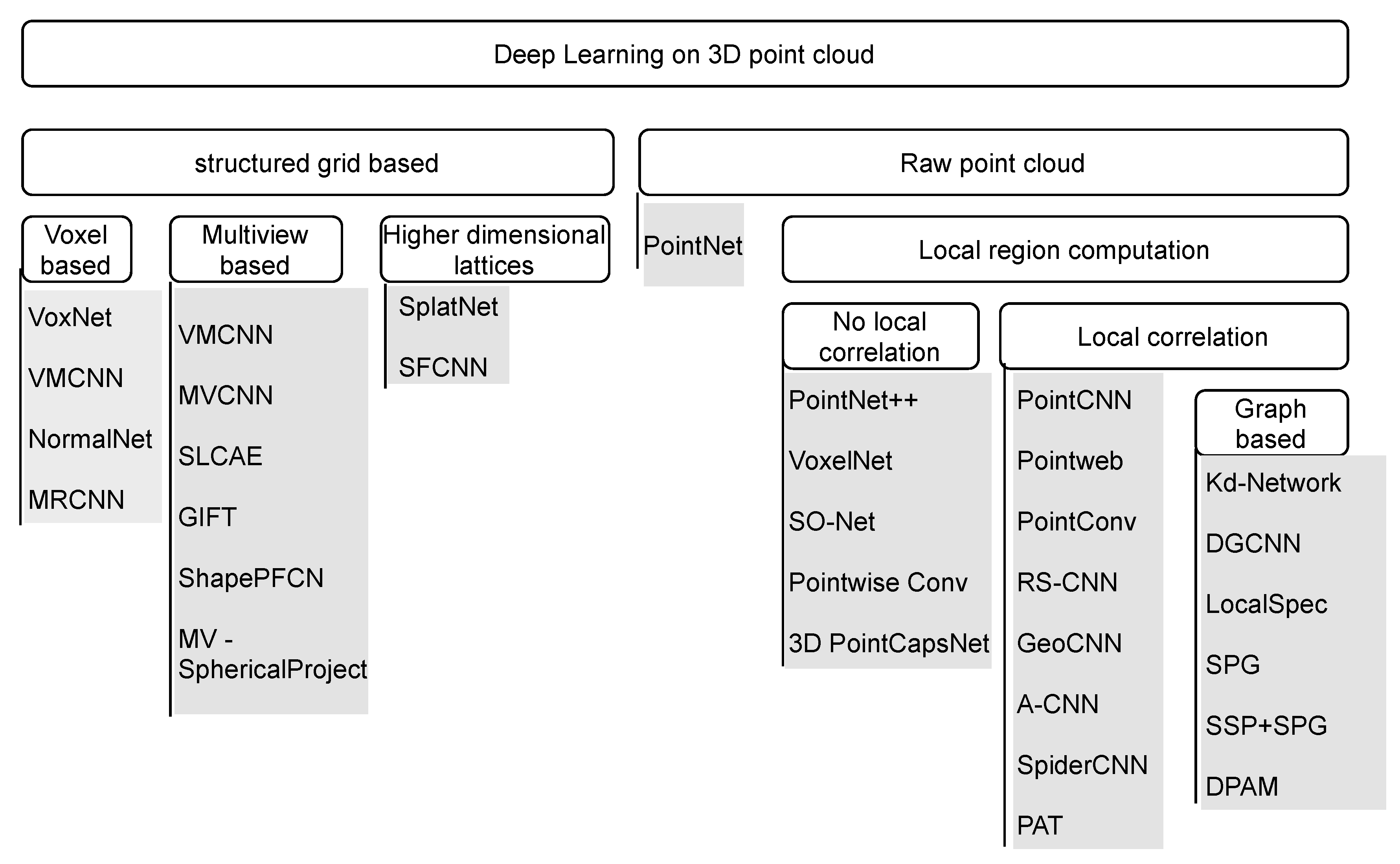
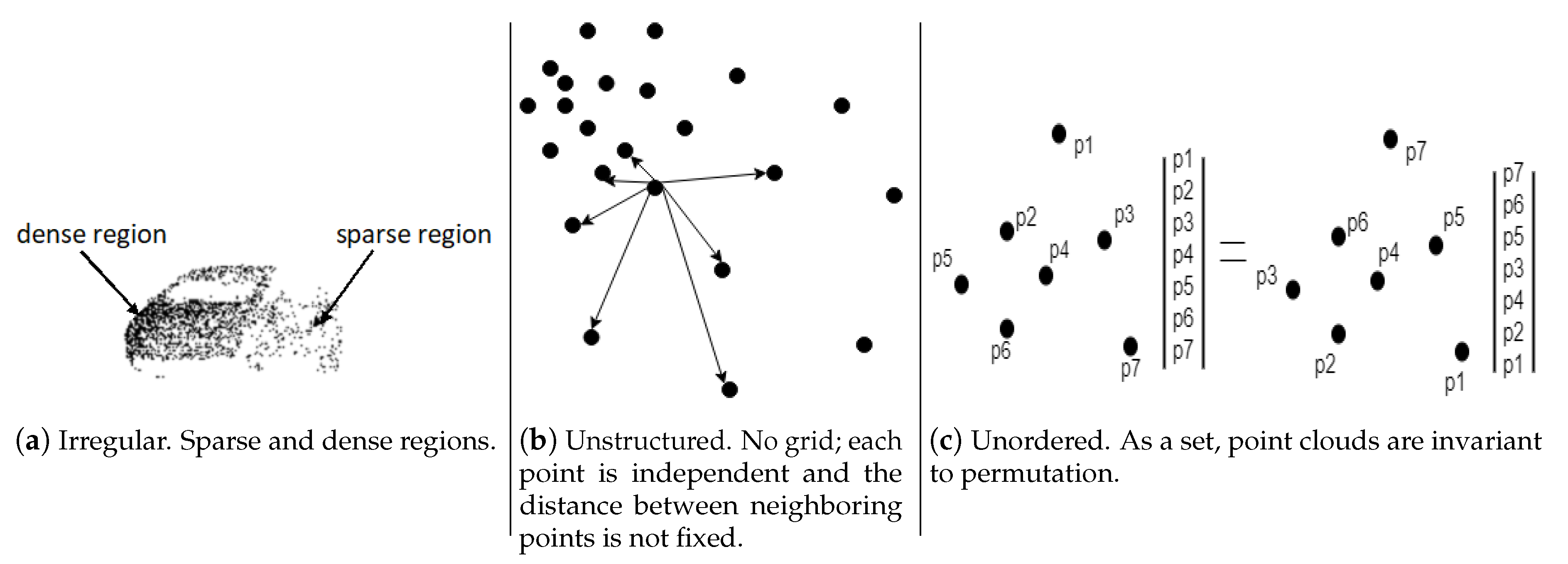
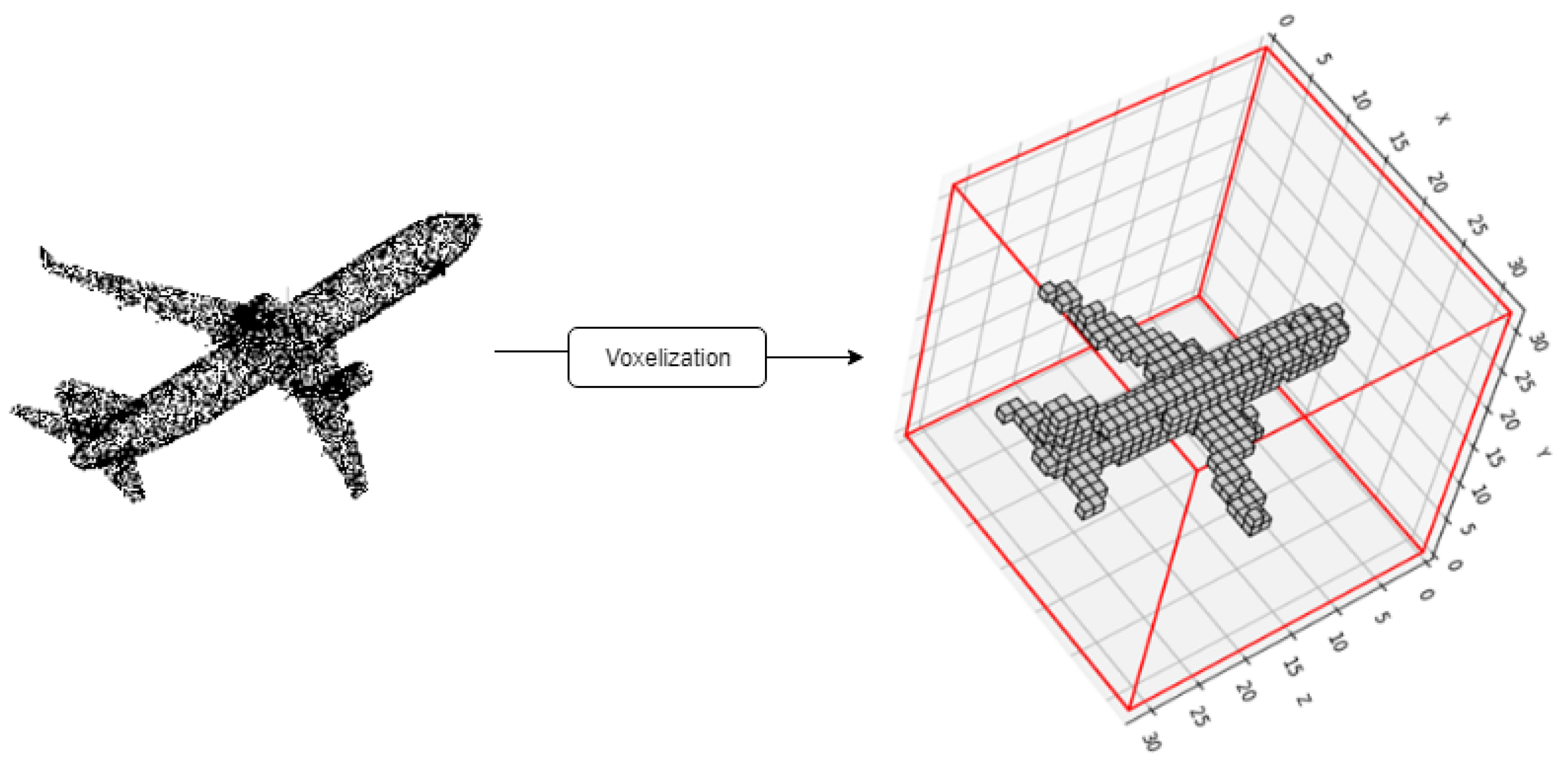
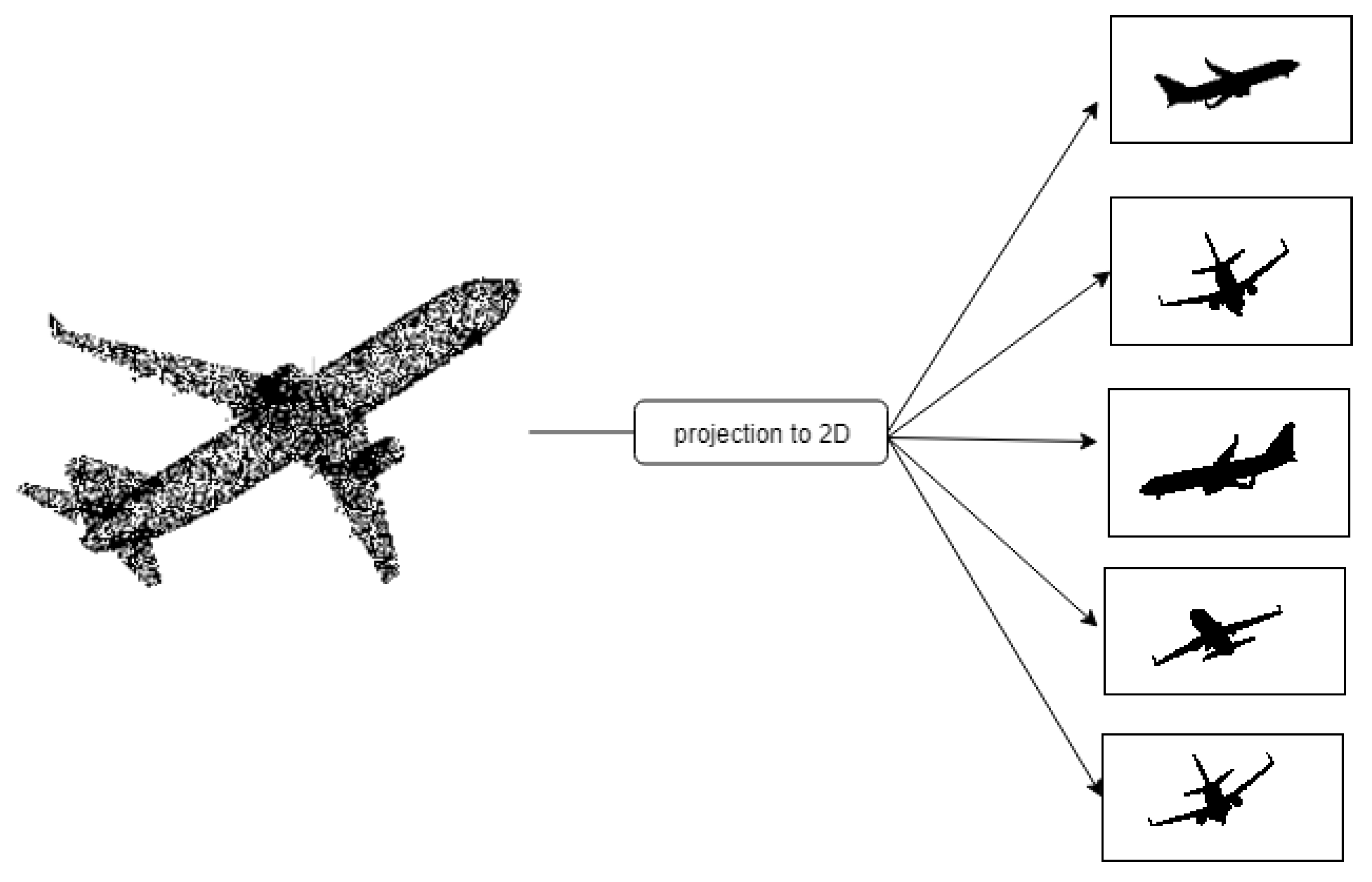
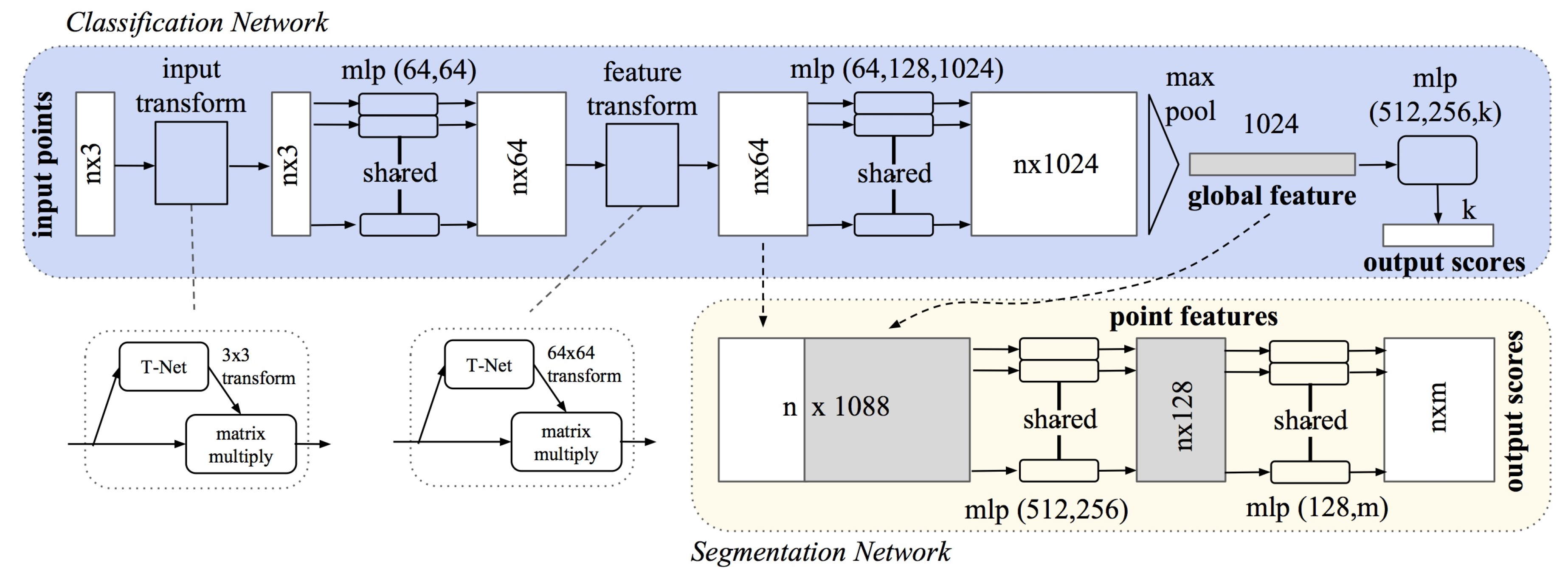
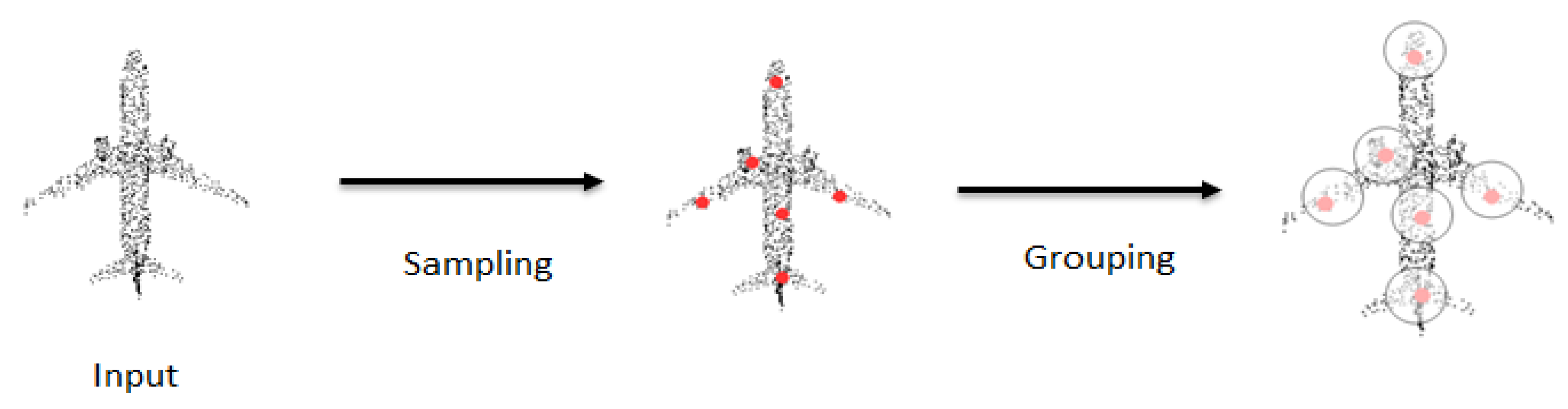
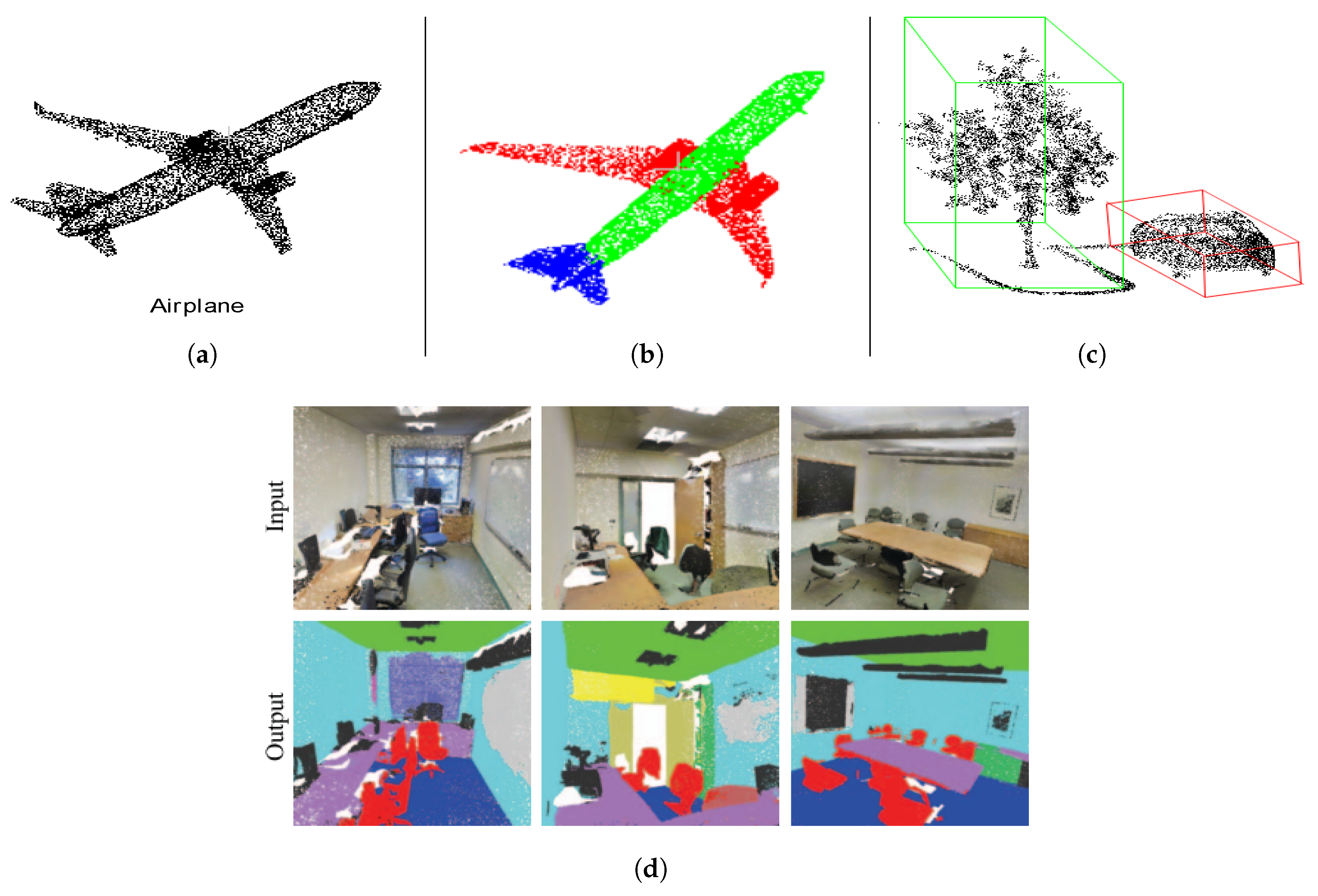
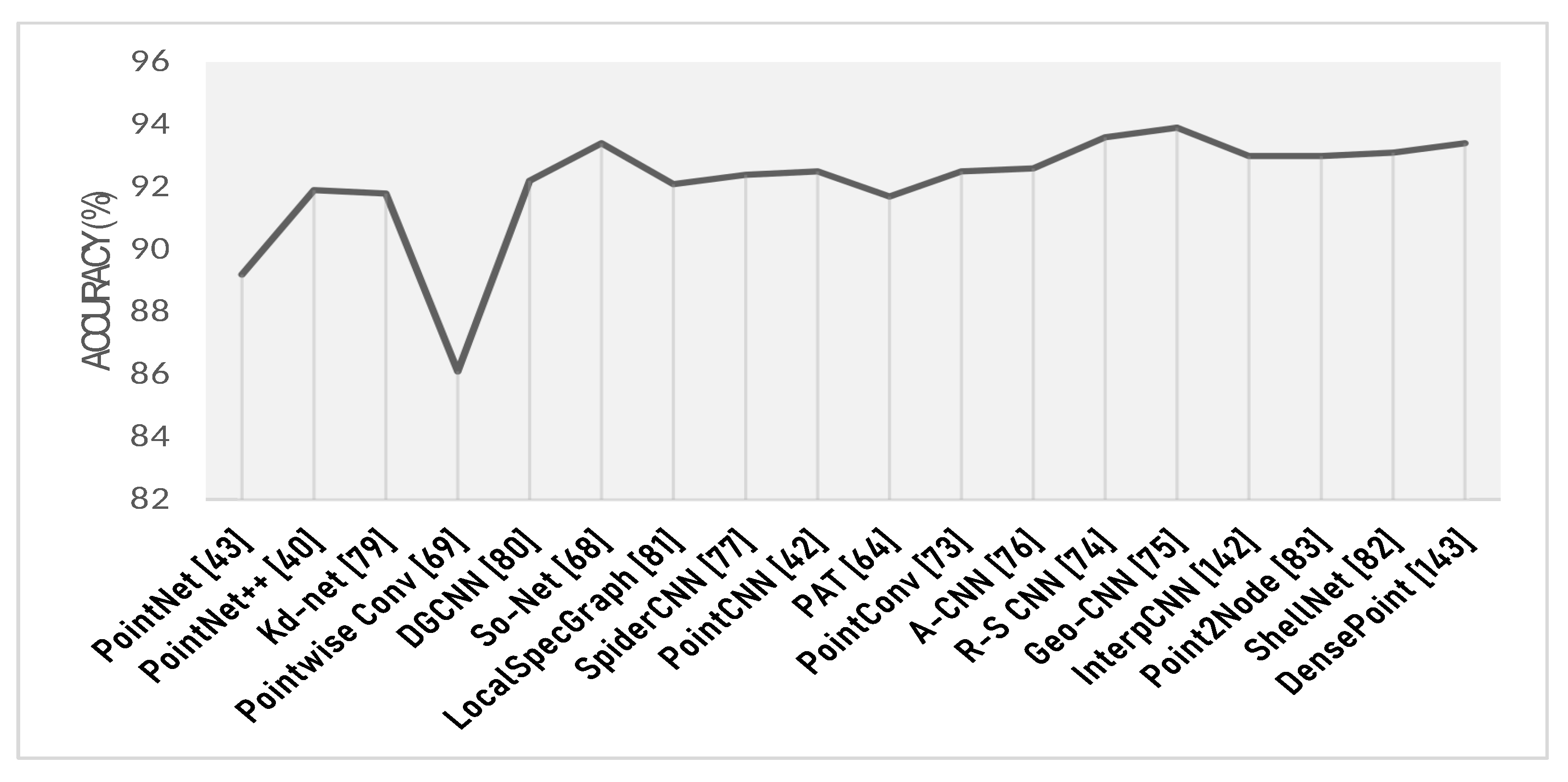
Table 1.
Summary of methods showing the sampling, grouping, and mapping functions used. CNN: convolutional neural network; DGCNN: dynamic graph CNN; SOM: self-organizing map; k-NN: k-nearest neighbor; MLP: multi-layer perceptron.
Table 1.
Summary of methods showing the sampling, grouping, and mapping functions used. CNN: convolutional neural network; DGCNN: dynamic graph CNN; SOM: self-organizing map; k-NN: k-nearest neighbor; MLP: multi-layer perceptron.
| Method | Sampling | Grouping | Mapping Function |
|---|---|---|---|
| PointNet [42] | - | - | MLP |
| PointNet++ [39] | Farthest point sampling | Radius-search | MLP |
| PointCNN [41] | Uniform/Random sampling | k-NN | MLP |
| So-Net [67] | SOM-Nodes | Radius-search | MLP |
| Pointwise Conv [68] | - | Radius-search | MLP |
| Kd-Network [78] | - | Tree based nodes | Affine transformations+ReLU |
| DGCNN [79] | - | k-NN | MLP |
| LocalSpec [80] | Farthest point sampling | k-NN | Spectral convolution + cluster pooling |
| SpiderCNN [76] | Uniform sampling | k-NN | Taylor expansion |
| R-S CNN [73] | Uniform sampling | Radius-nn | MLP |
| PointConv [72] | Uniform sampling | Radius-nn | MLP |
| PAT [63] | Gumbel subset sampling | k-NN | MLP |
| 3D-PointCapsNet [69] | - | - | MLP+Dynamic routing |
| A-CNN [75] | Uniform subsampling | k-NN | MLP+Density functions |
| ShellNet [86] | Random Sampling | Spherical Shells | 1D convolution |
Table 2.
Categorization of benchmark datasets. (cls: classification, seg: segmentation, loc: localization, reg: registration, aut: autonomous driving, det: object detection, dri: driving behavior, mot: motion estimation, odo: odometry, CAD: computer-assisted design, LiDAR: light detection and ranging.).
| Model | Indoor | Outdoor | ||
|---|---|---|---|---|
| CAD | ModelNet (2015, cls), ShapeNet (2015, seg), Augmenting ShapeNet, Shape2Motion (2019, seg, mot) | |||
| RGB-D | ScanObjectNN (2019, cls) | NYUDv2 (2012, seg), SUN3D (2013, seg), S3DIS (2016, seg), SceneNN (2016, seg), ScanNet (2017, seg), Matterport3D (2017, seg), 3DMatch (2017, reg) | ||
| LiDAR | Terrestrial LiDAR scanning | Semantic3D (2017, seg) | ||
| Mobile LiDAR scanning | Multisensor Indoor Mapping and Positioning Dataset (2018, loc) | KITTI (2012, det, odo), Semantic KITTI (2019, seg), ASL Dataset (2012, reg), iQmulus (2014, seg), Oxford Robotcar (2017, aut), NCLT (2016, aut), DBNet (2018, dri),NPM3D (2017, seg), Apollo (2018, det, loc), nuScenes (2019, det, aut), BLVD (2019, det) Whu-TLS (2020, reg) | ||
Table 3.
Details of benchmark datasets.
| Dataset | Dataset Capacity | Classification Categories | Segmentation Categories | Object Detection Categories | |
|---|---|---|---|---|---|
| CAD | ModelNet [48] | CAD models | 40 | ||
| ShapeNet [87] | models | 3135 | |||
| Shape2Motion [94] | models | 45 | |||
| RGB-D | ScanObjectNN [96] | objects | 15 | ||
| NYUDv2 [98] | RGB-D images | ||||
| SUN3D [100] | 254 different spaces | ||||
| S3DIS [101] | Over points | 13 | |||
| SceneNN [97] | 101 indoor scenes | 40 | |||
| ScanNet [64] | Nearly RGB-D images | 17 | 20 | ||
| Matterport3D [104] | RGB-D images | ||||
| 3DMatch [105] | 62 indoor scenes | ||||
| LiDAR | Semantic3D [126] | Over 4 billion points | 8 | ||
| MIMP [110] | Over points | ||||
| KITTI odometyr [111] | 22 sequences | ||||
| Semantic KITTI [115] | 22 sequences | 28 | |||
| ASL Dataset [116] | 8 sequences | ||||
| iQmulus [119] | points | 50 | |||
| Oxford Robotcar [121] | 100 sequences | ||||
| NCLT [123] | 27 sequences | ||||
| DBNet [127] | km driving data | ||||
| NPM3D [128] | points | 50 | |||
| Apollo [129,130] | images | More than car instances | |||
| nuScenes [133] | driving scenes | 23 classes and 8 attributes | |||
| BLVD [134] | 654 video clips | 3D annotations | |||
| Whu-TLS [135] |
Table 4.
Parts segmentation on the ShapeNet part dataset. The score is the mean intersection over union (mIOU).
Table 4.
Parts segmentation on the ShapeNet part dataset. The score is the mean intersection over union (mIOU).
| Method | Score (%) |
|---|---|
| PointNet [42] | 83.7 |
| PointCNN [41] | 84.6 |
| So-Net [67] | 84.6 |
| PointConv [72] | 85.7 |
| Kd-Network [78] | 82.3 |
| DGCNN [79] | 85.2 |
| LocalSpec [80] | 85.4 |
| SpiderCNN [76] | 85.3 |
| R-S CNN [73] | 86.1 |
| A-CNN [75] | 86.1 |
| ShellNet [86] | 82.8 |
| InterpCNN [141] | 84.0 |
| DensePoint [142] | 84.2 |
Table 5.
Semantic segmentation on S3DIS and ScanNet datasets. OA: overall accuracy.
| Method | Datasets | Measure | Score (%) |
|---|---|---|---|
| PointNet [42] | mIOU | 47.7 | |
| Pointwise Conv [68] | 56.1 | ||
| DGCNN [79] | 56.1 | ||
| PointCNN [41] | 65.4 | ||
| PAT [63] | 54.3 | ||
| ShellNet [86] | 66.8 | ||
| Point2Node [81] | S3DIS | 70.0 | |
| InterpCNN [141] | 66.7 | ||
| PointNet [42] | OA | 78.5 | |
| PointCNN [41] | 88.1 | ||
| DGCNN [79] | 84.1 | ||
| A-CNN [75] | 87.3 | ||
| JSIS3D [143] | 87.4 | ||
| PointNet++ [39] | mIOU | 55.7 | |
| PointNet [42] | 33.9 | ||
| PointConv [72] | 55.6 | ||
| PointCNN [41] | 45.8 | ||
| PointNet [42] | ScanNet | OA | 73.9 |
| PointCNN [41] | 85.1 | ||
| A-CNN [75] | 85.4 | ||
| LocalSpec [80] | 85.4 | ||
| PointNet++ [39] | 84.5 | ||
| ShellNet [86] | 85.2 | ||
| Point2Node [81] | 86.3 |
Table 6.
Instance segmentation on the ScanNet dataset. The measure is mean average precision (AP) at an overlap of 0.5 (50%).
Table 6.
Instance segmentation on the ScanNet dataset. The measure is mean average precision (AP) at an overlap of 0.5 (50%).
| Method | Avg AP 50% | Bath -Tub | Bed | Book -Shelf | Cabi -Net | Chair | Coun -Ter | Curt -Ain | Desk | Door | Picture | Refrig -Erator | Shower Curtain | Sink |
|---|---|---|---|---|---|---|---|---|---|---|---|---|---|---|
| 3D-MPA [148] | 0.611 | 1.00 | 0.833 | 0.765 | 0.526 | 0.756 | 0.136 | 0.588 | 0.47 | 0.438 | 0.358 | 0.65 | 0.857 | 0.429 |
| MTML [149] | 0.549 | 1.00 | 0.807 | 0.588 | 0.327 | 0.647 | 0.004 | 0.815 | 0.18 | 0.418 | 0.182 | 0.445 | 1.00 | 0.442 |
| 3D-BoNet [144] | 0.488 | 1.00 | 0.672 | 0.59 | 0.301 | 0.484 | 0.098 | 0.62 | 0.306 | 0.341 | 0.125 | 0.434 | 0.796 | 0.402 |
| PanopticFusion-inst [150] | 0.478 | 0.667 | 0.712 | 0.595 | 0.259 | 0.55 | 0.00 | 0.613 | 0.175 | 0.25 | 0.437 | 0.411 | 0.857 | 0.485 |
| ResNet-backbone [151] | 0.459 | 1.00 | 0.737 | 0.159 | 0.259 | 0.587 | 0.138 | 0.475 | 0.217 | 0.416 | 0.128 | 0.315 | 0.714 | 0.411 |
| MASC [152] | 0.447 | 0.528 | 0.555 | 0.381 | 0.382 | 0.633 | 0.002 | 0.509 | 0.26 | 0.361 | 0.327 | 0.451 | 0.571 | 0.367 |
| 3D-SIS [153] | 0.382 | 1.00 | 0.432 | 0.245 | 0.19 | 0.577 | 0.013 | 0.263 | 0.033 | 0.32 | 0.075 | 0.422 | 0.857 | 0.117 |
| UNet-backbone [151] | 0.319 | 0.667 | 0.715 | 0.233 | 0.189 | 0.479 | 0.008 | 0.218 | 0.067 | 0.201 | 0.107 | 0.123 | 0.438 | 0.15 |
| R-PointNet [145] | 0.306 | 0.5 | 0.405 | 0.311 | 0.348 | 0.589 | 0.054 | 0.068 | 0.126 | 0.283 | 0.028 | 0.219 | 0.214 | 0.331 |
| 3D-BEVIS [154] | 0.248 | 0.667 | 0.566 | 0.076 | 0.035 | 0.394 | 0.027 | 0.035 | 0.098 | 0.099 | 0.025 | 0.098 | 0.375 | 0.126 |
| Seg-Cluster [146] | 0.215 | 0.37 | 0.337 | 0.285 | 0.105 | 0.325 | 0.025 | 0.282 | 0.085 | 0.105 | 0.007 | 0.079 | 0.317 | 0.114 |
| Sgpn_scannet [146] | 0.143 | 0.208 | 0.39 | 0.169 | 0.065 | 0.275 | 0.029 | 0.069 | 0.00 | 0.087 | 0.014 | 0.027 | 0.00 | 0.112 |
| MaskRCNN 2d->3d Proj [155] | 0.058 | 0.333 | 0.002 | 0.00 | 0.053 | 0.002 | 0.002 | 0.021 | 0.00 | 0.045 | 0.238 | 0.065 | 0.00 | 0.014 |
Table 7.
Performance on the KITTI Bird’s Eye View detection benchmark.
| Method | Modality | Speed (HZ) | mAP | Car | Pedestrian | Cyclist | ||||||
|---|---|---|---|---|---|---|---|---|---|---|---|---|
| Moderate | Easy | Moderate | Hard | Easy | Moderate | Hard | Easy | Moderate | Hard | |||
| MV3D [168] | LiDAR & Image | 2.8 | N/A | 86.02 | 76.9 | 68.49 | N/A | N/A | N/A | N/A | N/A | N/A |
| Cont-Fuse [169] | LiDAR & Image | 16.7 | N/A | 88.81 | 85.83 | 77.33 | N/A | N/A | N/A | N/A | N/A | N/A |
| Roarnet [170] | LiDAR & Image | 10 | N/A | 88.2 | 79.41 | 70.02 | N/A | N/A | N/A | N/A | N/A | N/A |
| AVOD-FPN [171] | LiDAR & Image | 10 | 64.11 | 88.53 | 83.79 | 77.9 | 58.75 | 51.05 | 47.54 | 68.09 | 57.48 | 50.77 |
| F-PointNet [163] | LiDAR & Image | 5.9 | 65.39 | 88.7 | 84 | 75.33 | 58.09 | 50.22 | 47.2 | 75.38 | 61.96 | 54.68 |
| HDNET [172] | LiDAR & Map | 20 | N/A | 89.14 | 86.57 | 78.32 | N/A | N/A | N/A | N/A | N/A | N/A |
| PIXOR++ [173] | LiDAR | 35 | N/A | 89.38 | 83.7 | 77.97 | N/A | N/A | N/A | N/A | N/A | N/A |
| VoxelNet [65] | LiDAR | 4.4 | 58.52 | 89.35 | 79.26 | 77.39 | 46.13 | 40.74 | 38.11 | 66.7 | 54.76 | 50.55 |
| SECOND [174] | LiDAR | 20 | 60.56 | 88.07 | 79.37 | 77.95 | 55.1 | 46.27 | 44.76 | 73.67 | 56.04 | 48.78 |
| PointRCNN [164] | LiDAR | N/A | N/A | 89.28 | 86.04 | 79.02 | N/A | N/A | N/A | N/A | N/A | N/A |
| PointPillars [166] | LiDAR | 62 | 66.19 | 88.35 | 86.1 | 79.83 | 58.66 | 50.23 | 47.19 | 79.14 | 62.25 | 56 |
Table 8.
Performance on the KITTI 3D object detection benchmark.
| Method | Modality | Speed (HZ) | mAP | Car | Pedestrian | Cyclist | ||||||
|---|---|---|---|---|---|---|---|---|---|---|---|---|
| Moderate | Easy | Moderate | Hard | Easy | Moderate | Hard | Easy | Moderate | Hard | |||
| MV3D [168] | LiDAR & Image | 2.8 | N/A | 71.09 | 62.35 | 55.12 | N/A | N/A | N/A | N/A | N/A | N/A |
| Cont-Fuse [169] | LiDAR & Image | 16.7 | N/A | 82.54 | 66.22 | 64.04 | N/A | N/A | N/A | N/A | N/A | N/A |
| Roarnet [170] | LiDAR & Image | 10 | N/A | 83.71 | 73.04 | 59.16 | N/A | N/A | N/A | N/A | N/A | N/A |
| AVOD-FPN [171] | LiDAR & Image | 10 | 55.62 | 81.94 | 71.88 | 66.38 | 50.8 | 42.81 | 40.88 | 64 | 52.18 | 46.64 |
| F-PointNet [163] | LiDAR & Image | 5.9 | 57.35 | 81.2 | 70.39 | 62.19 | 51.21 | 44.89 | 40.23 | 71.96 | 56.77 | 50.39 |
| VoxelNet [65] | LiDAR | 4.4 | 49.05 | 77.47 | 65.11 | 57.73 | 39.48 | 33.69 | 31.5 | 61.22 | 48.36 | 44.37 |
| SECOND [174] | LiDAR | 20 | 56.69 | 83.13 | 73.66 | 66.2 | 51.07 | 42.56 | 37.29 | 70.51 | 53.85 | 46.9 |
| PointRCNN [164] | LiDAR | N/A | N/A | 84.32 | 75.42 | 67.86 | N/A | N/A | N/A | N/A | N/A | N/A |
| PointPillars [166] | LiDAR | 62 | 59.2 | 79.05 | 74.99 | 68.3 | 52.08 | 43.53 | 41.49 | 75.78 | 59.07 | 52.92 |
© 2020 by the authors. Licensee MDPI, Basel, Switzerland. This article is an open access article distributed under the terms and conditions of the Creative Commons Attribution (CC BY) license (http://creativecommons.org/licenses/by/4.0/).
Share and Cite
MDPI and ACS Style
Bello, S.A.; Yu, S.; Wang, C.; Adam, J.M.; Li, J. Review: Deep Learning on 3D Point Clouds. Remote Sens. 2020, 12, 1729. https://0-doi-org.brum.beds.ac.uk/10.3390/rs12111729
AMA Style
Bello SA, Yu S, Wang C, Adam JM, Li J. Review: Deep Learning on 3D Point Clouds. Remote Sensing. 2020; 12(11):1729. https://0-doi-org.brum.beds.ac.uk/10.3390/rs12111729
Chicago/Turabian StyleBello, Saifullahi Aminu, Shangshu Yu, Cheng Wang, Jibril Muhmmad Adam, and Jonathan Li. 2020. "Review: Deep Learning on 3D Point Clouds" Remote Sensing 12, no. 11: 1729. https://0-doi-org.brum.beds.ac.uk/10.3390/rs12111729
Note that from the first issue of 2016, this journal uses article numbers instead of page numbers. See further details here.