Hybrid Fusion-Based Background Segmentation in Multispectral Polarimetric Imagery

Abstract

Multispectral Polarimetric Imagery (MSPI) contains significant information about an object’s distribution, shape, shading, texture and roughness features which can distinguish between foreground and background in a complex scene. Due to spectral signatures being limited to material properties, Background Segmentation (BS) is a difficult task when there are shadows, illumination and clutter in a scene. In this work, we propose a two-fold BS approach: multiband image fusion and polarimetric BS. Firstly, considering that the background in a scene is polarized by nature, the spectral reflectance and correlations and the textural features of MSPI are calculated and analyzed to demonstrate the fusion significance. After that, integrating Principal Component Analysis (PCA) with Fast Fourier Transform (FFT), a hybrid fusion technique is proposed to show the multiband fusion effectiveness. Secondly, utilizing the Stokes vector, polarimetric components are calculated to separate a complex scene’s background from its foreground by constructing four significant foreground masks. An intensity-invariant mask is built by differentiating between the median filtering versions of unpolarized and polarized images. A strongly unpolarized foreground mask is also constructed in two different ways, through analyzing the Angle of Linear Polarization (AoLP) and Degree of Linear Polarization (DoLP). Moreover, a strongly polarized mask and a strong light intensity mask are also calculated based on the azimuth angle and the total light intensity. Finally, all these masks are combined, and a morphological operation is applied to segment the final background area of a scene. The proposed two-fold BS algorithm is evaluated using distinct statistical measurements and compared with well-known fusion methods and BS methods highlighted in this paper. The experimental results demonstrate that the proposed hybrid fusion method significantly improves multiband fusion quality. Furthermore, the proposed polarimetric BS approach also improves the mean accuracy, geometric mean and F1-score to 0.95, 0.93 and 0.97, respectively, for scenes in the MSPI dataset compared with those obtained from the methods in the literature considered in this paper. Future work will investigate mixed polarized and unpolarized BS in the MSPI dataset with specular reflection.

1. Introduction

The emerging significance of Multispectral Polarimetric Imagery (MSPI) has been actively pursued in diverse applications over the last few decades. Using advanced communication tools and techniques, multispectral images are currently composed of several sub-bands from both the visible and near infrared (NIR) wavelengths [1], with the latter material-dependent and capable of penetrating deeper into materials. Potential applications could investigate acquiring an imaging system that performs image denoising [2], image dehazing [3] and semantic segmentation [4]. Multispectral imaging is a mode commonly reported in the literature for enhancing color reproduction [5], illuminant estimation [6], vegetation phenology [7,8], shadow detection [9] and background subtraction [10]. However, based on only multispectral information, it is sometimes unfeasible to segment the background from a complex scene, whereas polarimetric imagery is shown to extract meaningful information about surface features, shapes, shading and smoothness in optical sensing images [11]. Specific photoreceptors are responsible for polarized light vision, a phenomenon used by polarimetric imaging techniques in diverse applications, such as specular and diffuse separation [12], material classification [13], shape estimation [14], target detection [15,16,17], anomaly detection [18], man-made object separation [19] and camouflaged object separation [20].

Currently, computer vision-based Background Segmentation (BS) has potential application for shape detection, activity detection and recognition, behavioral understanding, surveillance, medical care and parenting [21]. However, an error in object detection can degrade the overall performance of a system. In terms of surveillance and monitoring systems, the foreground in a scene is described as a disruptor that breaks up the background. Existing approaches [22,23] based on this criterion first look for a region of interest to segment the background from a scene, with their performances reported to depend on the contrast between an object and its background. Although a frame-differencing approach may sometimes be beneficial for BS, selecting an appropriate threshold is a challenging task due to the foreground and background sometimes being mixed in a complex scene. Given fast processing power and a noise-handling capacity, an average image of a series of N bands can be calculated to predict a difference image. However, challenges, including low lighting conditions, illumination, occluded foreground and shadow effects, which can be camouflaged in an imaging modality, including the visible light spectrum, need to be considered.

Although integrating data captured from multiple spectra followed by different polarization filter orientations benefits a BS task, registering multispectral acquisitions is more challenging [24]. Combining six bands of multispectral images in a spectrum (420–1000 nm) and four different orientations of linear polarization filters ($0^{°}, {45}^{°}, {90}^{°}, {135}^{°}$) can improve the accuracy of a BS technique. In this paper, to address the problem of the dissimilarity of multiband information, a multiband fusion framework with an algorithm is proposed. Firstly, the fusion algorithm decomposes each band into low- and high-frequency components and then the first Principal Component (PC) of each side is calculated. This proposed automatic approach does not require either prior knowledge of the foreground objects in a scene or a background model. After the polarimetric components are calculated, four different foreground masks are generated to distinguish between the foreground and background.

The main contribution of this research is two-fold. Firstly, a hybrid fusion technique for fusing information from multiple spectra with different polarimetric orientation images is proposed. This stage is composed of a Fast Fourier Transform (FFT) and Principal Component Analysis (PCA), with each spectrum initially decomposed into low and high frequencies. Then, the first Principal Component (PC) of each frequency is computed and combined to obtain a final fused image. Secondly, a polarimetric BS technique for segmenting a complex background from a scene is proposed. It uses polarimetric components to compute the significant foreground masks that are then combined through a morphological operation to produce the final background area of the scene. The proposed research aims to segment a background of a complex scene utilizing MSPI features. The performances of these approaches are evaluated and compared using a publicly available MSPI dataset to demonstrate the significance of this study.

This paper is organized as follows. In Section 2, the background to multiband fusion in MSPI is fully described. In Section 3, details of the MSPI dataset used are provided and the spectral reflectance, correlations and textural features for obtaining information dissimilarity are analyzed. In Section 4, a complete two-fold BS framework and algorithm are presented. A hybrid fusion algorithmic framework, polarimetric component processing and a polarimetric BS algorithm with significant steps and proper mathematical and logical explanations are also discussed. In Section 5, the performance of the proposed hybrid fusion method and accuracy of the proposed BS algorithm are evaluated and compared with those of existing approaches in this literature. An experiment on computational time for the proposed method is also presented and compared with other approaches in this section. Finally, concluding remarks and suggested future directions are provided in Section 6.

2. Related Works

BS techniques usually assume that the intensity of background pixels varies from that of other pixels in multiple spectra according to [25]:

$$M_{x,y, \lambda ,o_i}=\{\begin{array}{cc}1\hfill & \hfill if d\left(I_{x,y, \lambda ,o_i}, B_{x,y, \lambda ,o_i} \right)>{\tau }_G\\ 0\hfill & \hfill otherwise\end{array}$$

(1)

where ${\tau }_G$ is a global threshold, $M_{x,y, \lambda ,o_i}$, the final background mask at pixel ($x,y$) of a fused spectrum $\left(\lambda \right)$ image at a polarimetric orientation ($o_i$) and $d$ is the distance between the pixel of the predicted background ($B$) and that of the fused image in spectrum $\lambda$($I$) at orientation $o_i$. In this paper, the literature related to BS is reviewed in terms of multispectral fusion and polarimetric BS.

2.1. Fusion

In general, multispectral images contain both spectral and spatial redundancies. The former is defined by a high correlation among multiple spectra and the latter by the correlation among neighboring pixels. Multispectral fusion aims to reduce both these redundancies while destroying as little as possible of the original image’s information and is usually performed by transform compression. Individual techniques and their performances related to visible and infrared image fusion are discussed in recent literature [26,27,28]. Although, in a lossless image compression technique, images remain almost identical to their original versions, in a lossy one, a high compression ratio such as PCA [29,30,31,32,33], which is based on dimensionality reduction, is calculated according to the covariance matrix ($C$):

$$C=\frac{1}{N}{\displaystyle \sum }_{n=1}^N\left(X_n-\overline{X}\right){\left(X_n-\overline{X}\right)}^T$$

(2)

where $N$ is the number of spectral bands, $X_n$ is a vector containing the pixel intensities of the $n^{th}$ band image and $\overline{X}$ is the mean of $X_n$. The eigenvectors and eigenvalues are then computed from $C$, after that PCA scores also calculated and multiplied by those of the original pixel intensities of the band images to obtain the first PC as a fused image [28]. Through applying PCA, Bavirisetti [34] has proposed edge-preserving Fourth-order Partial Differential Equations (FPDEs) to fuse multisensor images. Despite the advantage over energy compaction of the decorrelated spectral bands, the dependence on data to calculate the $C$ among the spectral bands is a disadvantage of PCA.

Due to the energy balance and registration problem existing in a multispectral data acquisition system, the appearances of objects demonstrate low correlations in different spectral bands [35]. However, multispectral pixel-level and transform domain-based fusion can effectively present an overall dataset. The traditional pixel-level fusion averages (AVG) method [36] contains the information of multiple spectra and, although it is simple and fast, each band’s images participate equally in the fused image without their information considered. In contrast, transform domain-based fusion methods first decompose the source images into a sequence of sub-band ones through a specific mathematical transform structure and then apply some fusion rules to determine the so-called sub-band coefficients [3]. Finally, a fused image is formed using the corresponding inverse transform. Mathematical transforms, which are well known as Multiscale Geometric Analyses (MGAs) include the Discrete Wavelet Transform (DWT) [37,38,39], Shearlet Transform (SHT) and Discrete Cosine Transform-based Laplacian Pyramid (DCT–LP). The DWT generates four different coefficients: approximation, horizontal detail, vertical detail and diagonal detail, with a mean–maximum rule applied to fuse those of multiple spectra. Finally, an inverse transform is applied on all the final coefficients [27]. Although the DWT provides a higher signal-to-noise ratio (SNR) and better temporal resolution than other transforms, its performance depends on the number of decomposition levels.

In the SHT [20], two significantly different images (A and B) are selected from spectral bands which further decompose into some low- and many high-frequency coefficients (L_iA and H_iA, respectively). The mean of the low frequencies is the final low-frequency approximation coefficient (Equation (3)) and, by applying an area-based feature selection method (Equations (4) and (5)), the final high-frequency detail coefficients are calculated. Eventually, a fused image is obtained using an inverse SHT as follows.

$$L\left(x,y\right)=\frac{L_A\left(x,y\right)+L_B\left(x,y\right)}{2}$$

(3)

$$H_i\left(x,y\right)=\{\begin{array}{cc}{H}_i^A\left(x,y\right),\hfill & \hfill S_i^A\left(x,y\right)\ge S_i^B\left(x,y\right) \\ H_i^B\left(x,y\right),\hfill & \hfill otherwise\end{array}$$

(4)

where S is the weighted energy of the local window (Ω) calculated as:

$$S\left(x,y\right)={\left|f\left(x,y\right)\right|}^2 \frac{1}{Card\left(\Omega \right)}{\displaystyle \sum }_{\left(m,n\right)\in \Omega }{\left|f\left(m,n\right)\right|}^2$$

(5)

where $Card\left(\Omega \right)$ denotes the cardinality of a window (Ω) that is calculated by counting the number of distinct elements in the ($m,n$) coordinates. The advantage of the SHT is that it includes multiscale, shift-invariant and multidirectional image decompositions, but its computational complexity is significant.

In the DCT–LP [40], firstly, a Gaussian Pyramid (GP) is constructed with a reduced size of a band’s image and then the DCT and inverse DCT are applied on it, with an LP built by expanding the size of the previous image and then applying the DCT and inverse DCT on it. After constructing a k-level LP for individual images ($P_k^i \to \left\{g_k^i, l_0^i, l_1^i, \dots \dots , l_{k-1}^i \right\}, \mathrm{where} i=0, 1, \dots , N$), the fusion rule is

$$\mathrm{at} \mathrm{the} \mathrm{kth} \mathrm{level}, g_k^f=g_k^i/i$$

(6)

$$\mathrm{and}, \mathrm{at} \mathrm{the} \mathrm{k}-1 \mathrm{to} 0 \mathrm{levels}, g_{k-1}^f= l_{k-1}^f+E\left(g_k^f\right)$$

(7)

where $E\left(g_k^f\right)$ is an expanded function and $l_{k-1}^f=l_{k-1}^i$ if $\left|l_{k-1}^i\right|>\left|l_{k-1}^j\right|, \mathrm{where} j\ne i and j=0, 1, \dots ., N$. Despite its signal extension capability, the DCT suffers from poor image quality.

Therefore, considering the pros and cons of individual methods, we propose a holistic hybrid fusion approach for the lossy compression of multispectral images with high spatial resolutions by integrating an FFT with PCA.

2.2. Segmentation

Recent literature on multispectral polarized BS has focused mainly on binary (or foreground–background) segmentation [41] after fusion [42]. Without considering some constraints or assumptions, BS in multiband images seems to be very difficult due to an object appearing in some spectra exhibiting a low correlation [35]. Approaches based on monocular segmentation usually rely on the hypotheses of visual saliency (e.g., an object appearing in a scene is highly focused) or human oversight to achieve good results [43,44]. Given the additional assumptions that can be made about the motion of an object or scene, the same issue in the temporal domain (i.e., for image sequences) is easier to tackle. There are methods for motion clustering that depend on partitioning the optical flow or trajectory points to identify image regions that behave differently from their surroundings [45]. Also, the close correlation between motion partitioning and the segmentation of video objects has gained attention in the last decade [46,47].

Foreground–background separation is an easy task if the object of interest is available in multiple spectra. An example of the assumption of visual appearance is where common foreground objects are presented, and the background demonstrates low correlations in multiple spectra [48,49,50]. In contrast, methods for mutual segmentation usually assume that the same object is observed from multiple viewpoints and optimize the geometric consistency of the extracted foreground area [51,52,53]. Earlier mutual segmentation approaches which focus on single-spectrum imagery [53,54,55], with the registration problem solved using depth cameras [56,57], offer a range-based solution for detecting objects in a scene [51,52,58].

Currently, researchers are concentrating on combining spatial, spectral and polarimetric information to effectively predict the background and foreground in a scene without creating any background model. In some studies, color space mapping [13,20,29] is applied on fused multispectral polarimetric components and then fuzzy C-means clustering on separate objects from the background. Lu [59] applied PCA on different polarized images and then used a clustering technique to segment objects. These methods do not require any previous background model to segment the foreground/object from the background and are robust to illumination conditions. The proposed BS method creates some significant foreground masks from different polarimetric components and combines them to segment a complex background from a scene.

3. Analysis of the MSPI Dataset

Multispectral polarimetric data contain rich sets of information for discriminating foreground objects from the background in a complex scene.

3.1. Description of the Dataset

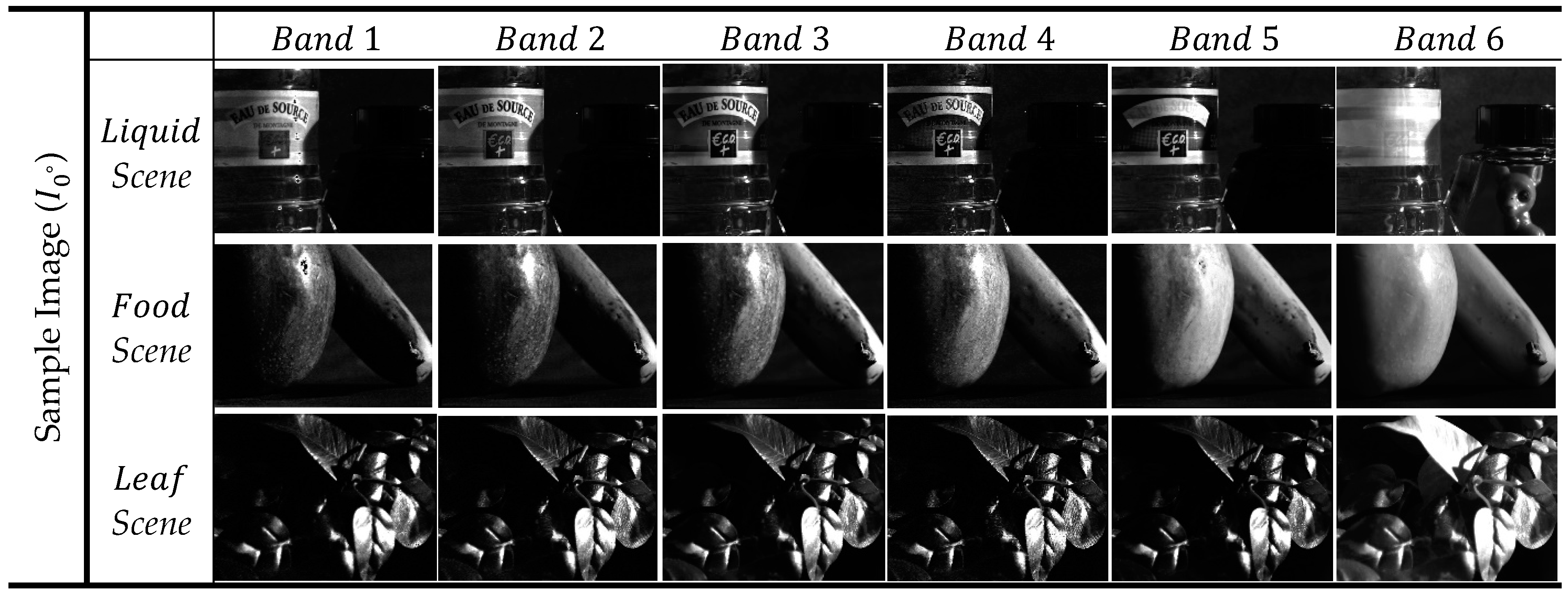
The multispectral polarimetric image dataset used in this paper is obtained from a publicly available one [60], which contains polarimetric and multispectral images from visible and near infrared (NIR) bands in the range of 420–1000 nm. The imaging system generates 10 different scenes in six spectral channels at four different polarimetric filter orientation angles ($0^{°}$, ${45}^{°}$, ${90}^{°}$, ${135}^{°}$). Of them, three scenes in which the background is polarized in nature are selected for our purpose. Samples of the dataset at $0^{°}$ polarimetric orientation ($I_{0^{°}}$) are shown in Figure 1, where the liquid scene is composed of reflecting objects, such as water in a bottle and a doll in a jar, the food scene of an apple and a banana, and the leaf scene of real and fake leaves with a mixed background.

3.2. Analysis of Spectral Reflectance

The camera response (${\rho }_i$) of the $i$^th channel is described by [1] as:

$${\rho }_i={\displaystyle \sum }_{\lambda =420}^{\lambda =1000}E\left(\lambda \right) R\left(\lambda \right) O\left(\lambda \right) C_i\left(\lambda \right)$$

(8)

where $E\left(\lambda \right)$ is the spectral emission of the illuminant, $R\left(\lambda \right)$ the reactance, $O\left(\lambda \right)$ the global transmittance of all the optical elements and $C_i\left(\lambda \right)$ the spectral sensitivity of the $i$^th channel. After calculating the measurement matrix (M), the spectral reflectance ($\widehat{R}$) is calculated as:

$$\widehat{R}=M^{-1}{\rho }_i$$

(9)

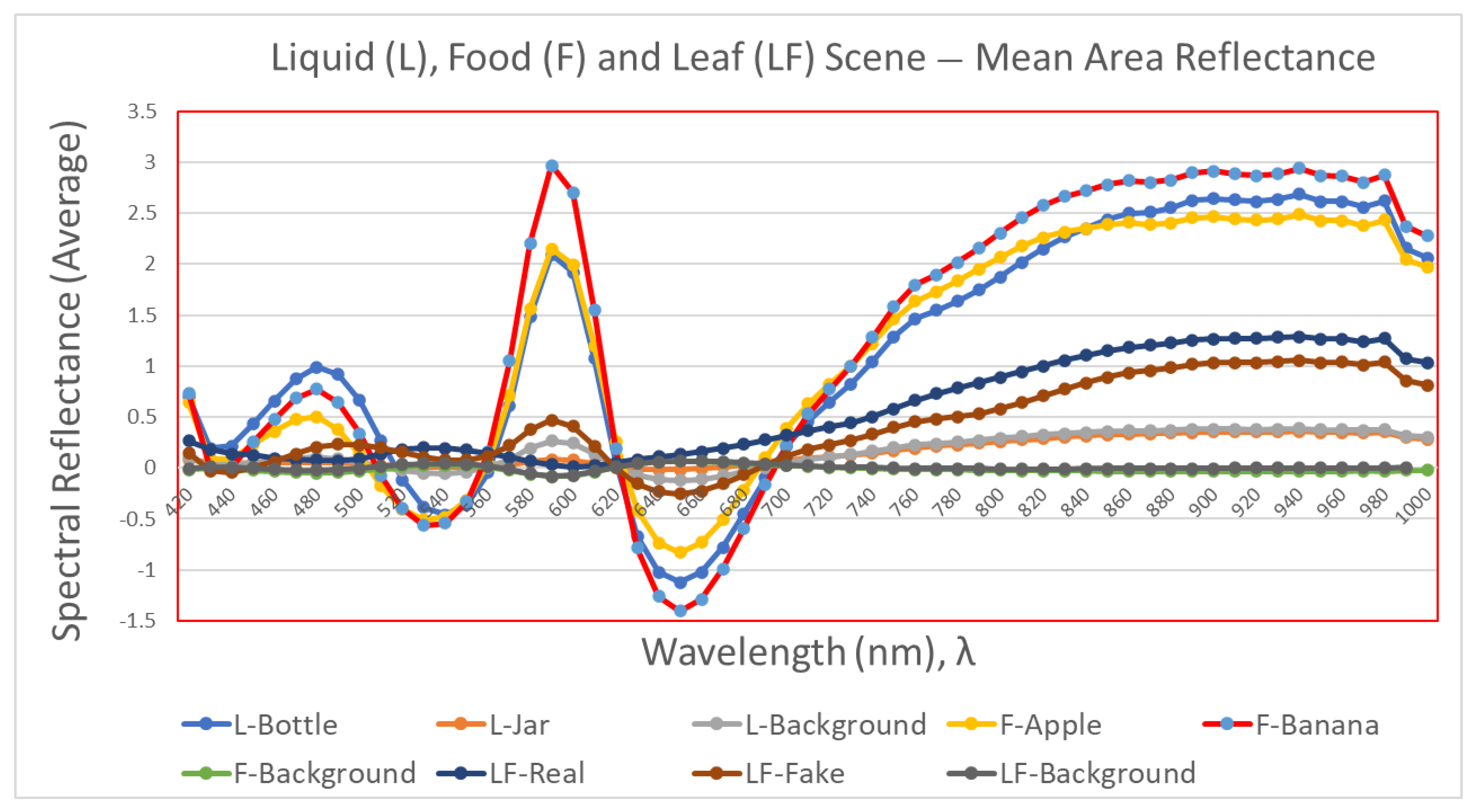
The mean spectral reflectance of an area demonstrates variations in information among multiple bands. It is also predicted that the foreground areas of different scenes, such as the liquid (L-Bottle, L-Jar), food (F-Apple, F-Banana) and leaf (LF-Real, LF-Fake) ones, exhibit higher spectral reflectance than their backgrounds as shown in Figure 2.

3.3. Analysis of Multiband the Dissimilarity Matrix

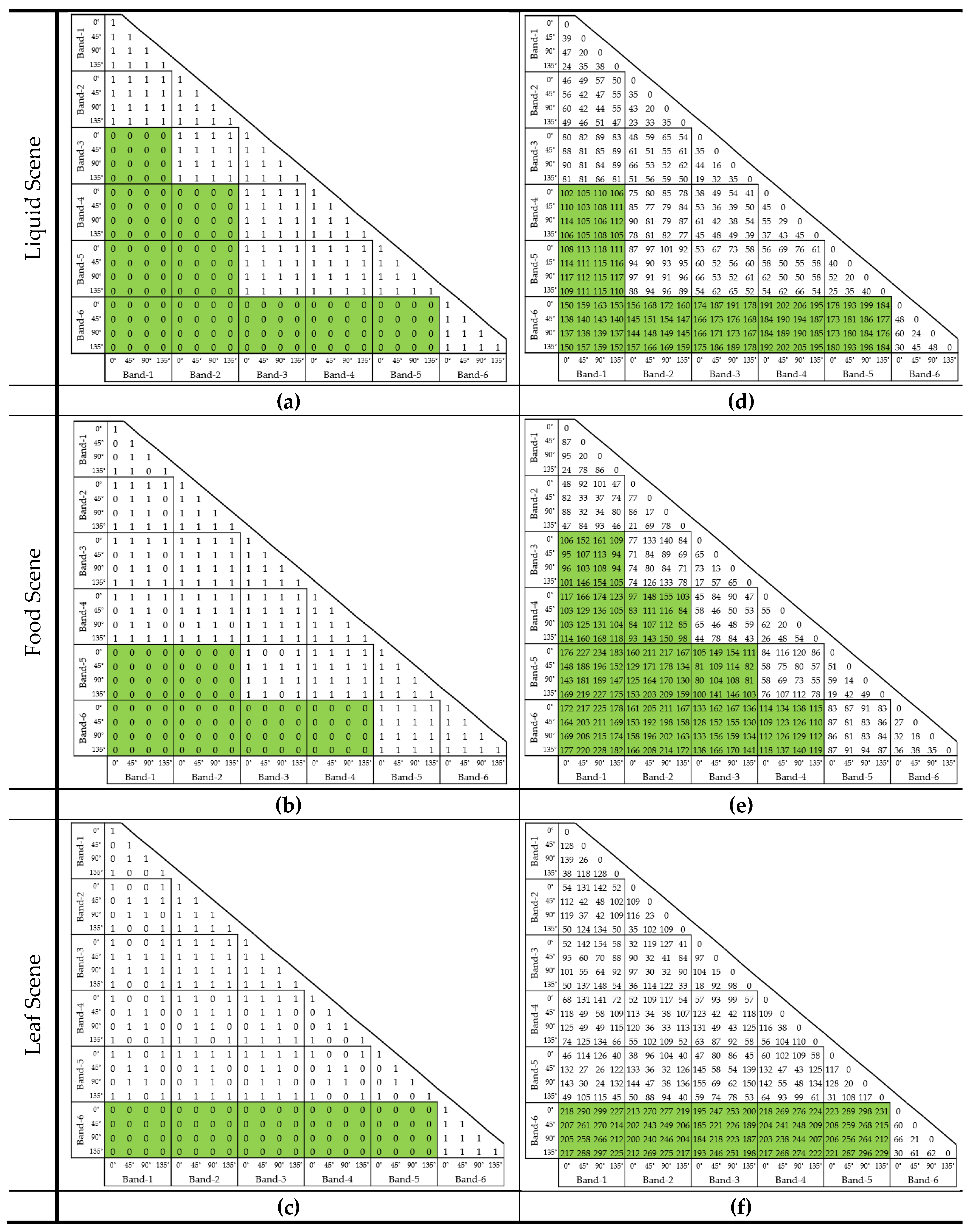
In MSPI, the data redundancies that can occur in spectral bands denote that one band’s data can be partly or fully predicted from those of the others. Multiband dissimilarity is calculated in two different ways, by the Pearson correlation and Euclidean distance. We consider three different MSPI scenes to compute their dissimilarity levels in multiple spectra.

3.3.1. Pearson Correlation

Higher correlations among multiple spectra demonstrate highly redundant information. To measure an inherent correlation between two images ($A_{mn}$ and $B_{mn}$), the Pearson correlation coefficient ($r$) is calculated as:

$$r=\frac{{{\displaystyle \sum }}_m{{\displaystyle \sum }}_n\left(A_{mn}-\overline{A}\right) \left(B_{mn}-\overline{B}\right)}{\sqrt{({{\displaystyle \sum }}_m{{\displaystyle \sum }}_n {\left(A_{mn}-\overline{A}\right)}^2) ({{\displaystyle \sum }}_m{{\displaystyle \sum }}_n {\left(B_{mn}-\overline{B}\right)}^2)}}$$

(10)

where $\overline{A}=\frac{1}{N}{{\displaystyle \sum }}_{i=0}^{N-1}{A}_{mn} \mathrm{and} \overline{B}=\frac{1}{N}{{\displaystyle \sum }}_{i=0}^{N-1}{B}_{mn}$.

The correlation matrices in the MSPI scenes due to the multiple spectra and multiple polarimetric orientations are presented in Figure 3a–c [61]. As can be seen, band 6 in the liquid and leaf scenes is not correlated with the other bands, while band 6 in the food scene is correlated with only band 5 above a threshold of 0.90. The bands not strongly correlated are indicated in green.

3.3.2. Euclidean Distance

To measure the distances among multiple spectra, the classical method used is the Euclidian distance that, between two images ($A_{mn}$ and $B_{mn}$), is calculated by:

$$d\left(A,B\right)=\sqrt{{\displaystyle \sum }_{i=0}^{m-1}{\displaystyle \sum }_{i=0}^{n-1}{\left(A_{mn}-B_{mn}\right)}^2}$$

(11)

and then normalized in the range (0–1). The distance matrices in the MSPI scenes due to the multiple spectra and different polarimetric orientations are presented in Figure 3d–f. As can be seen, band 6 is the most dissimilar to the others in the liquid and leaf scenes, while, in the food scene, bands 5 and 6 demonstrate similar information but are dissimilar to the others. The bands with large distances are indicated in green.

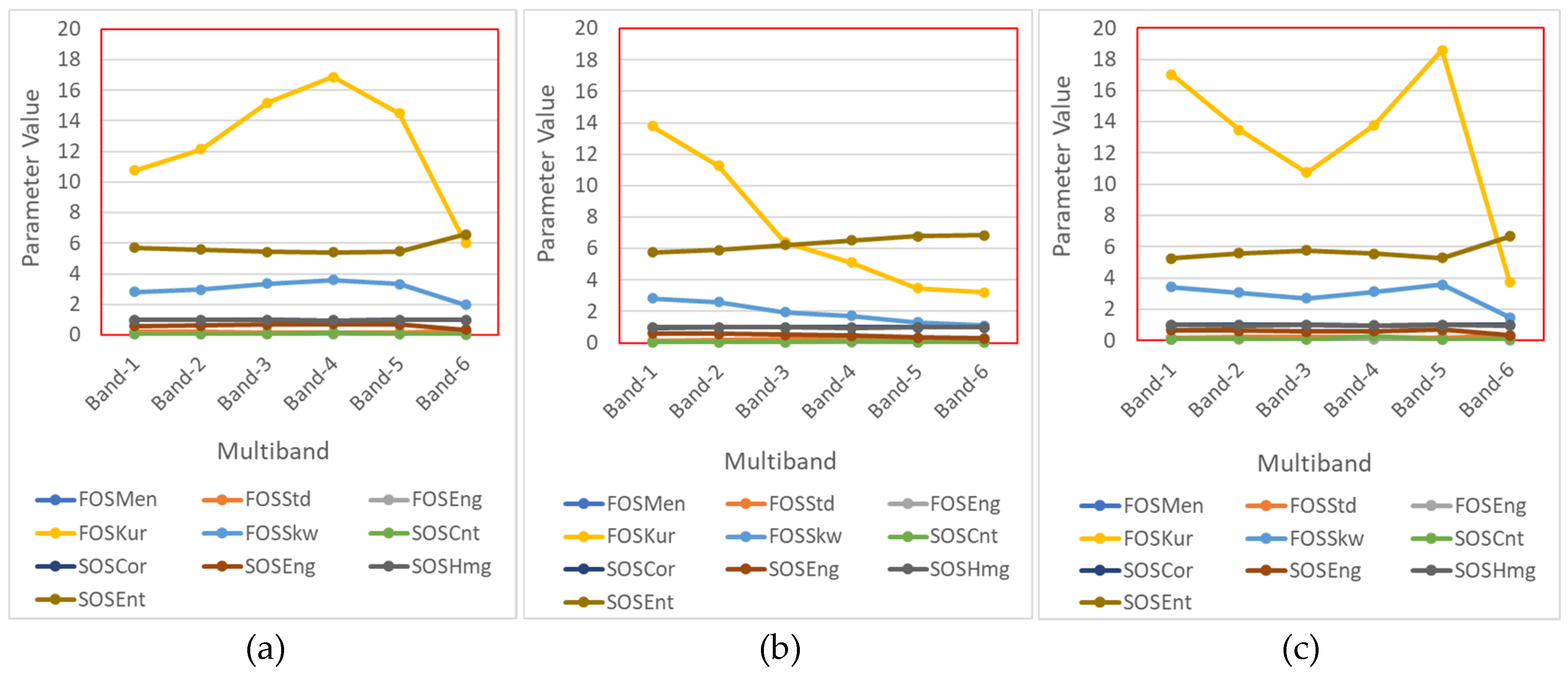
3.4. Analysis of Multiband Textural Features

In MSPI, textural features describe the local spatial variations in intensity as well as the homogeneity of images. They are divided into the two broad categories of first- and second-order statistical features, with the former dependent mainly on a histogram analysis of gray-level image representations. Considering $z_i$ as the gray value of the $i^{th}$ pixel, $P\left(z_i\right)$ is a normalized histogram and $N$ the number of distinctive gray levels, with the first-order histogram defined as [50]:

$$P\left(z_i\right)=\frac{number of pixels with value I}{number of total pixels}$$

(12)

The first-order statistical features are defined as follows [62].

1.	Mean is a measure of the spreading of the distribution from the mean value.	$\mathrm{FOSMen}, \mu ={\displaystyle {\displaystyle \sum }_{i=0}^{N-1}}{z}_i P\left(z_i\right)$	(13)
2.	Standard deviation is used to sharpen edges as the intensity level changes by a large value at the edge of an image.	$\mathrm{FOSStd}, \sigma =\sqrt{{\displaystyle {\displaystyle \sum }_{i=0}^{N-1}}{\left(z_i-\mu \right)}^2 P\left(z_i\right)}$	(14)
3.	Energy is a measure of the homogeneity of the histogram.	$\mathrm{FOSEng}, E={\displaystyle {\displaystyle \sum }_{i=0}^{N-1}}{\left(P\left(z_i\right)\right)}^2$	(15)
4.	Skewness is a measure of the degree of the histogram’s asymmetry around the mean.	$\mathrm{FOSSkw}, {\mu }_3=\frac{\frac{1}{N} {{\displaystyle \sum }}_{i=0}^{N-1}{\left(z_i-\mu \right)}^3 }{{\left(\sqrt{{{\displaystyle \sum }}_{i=0}^{N-1}\left(z_i{}^2- {\mu }^2 \right) }\right)}^3}$	(16)
5.	Kurtosis is a measure of the histogram’s sharpness, that is, whether the data are peaked or flat relative to a normal distribution.	$\mathrm{FOSKur}, {\mu }_4=\frac{\frac{1}{N} {{\displaystyle \sum }}_{i=0}^{N-1}{\left(z_i-\mu \right)}^4 }{{\left(\sqrt{{{\displaystyle \sum }}_{i=0}^{N-1}\left(z_i{}^2- {\mu }^2 \right) }\right)}^4}$	(17)

The second-order statistics or Gray-level Co-occurrence Matrix (GLCM) define a square matrix the size of which represents the probability of the gray value ($g_1$) being moved from a fixed spatial location relationship (size and direction) to another gray value ($g_2$). Assuming that $f\left(i_1,j_1\right)$ is a 2D gray-scale image, where $S$ is a set of pixels with a certain spatial relationship in the region and $P$ the GLCM, this is expressed as [63]:

$$P\left(i,j\right)=\frac{\#\left\{\left[\left(i_1,j_1\right),\left(i_2,j_2\right)\right]\in S|f\left(i_1,j_1\right)=g_1 \& f\left(i_2,j_2\right)=g_2\right\}}{\#S}$$

(18)

where $\#$ is used to define the quantity. The second-order statistical features are defined as follows.

1.	Contrast is a measure of the local variations present in an image, that is, it reflects the depth and smoothness of the image’s textural structure.	$\mathrm{SOSCon}={\displaystyle {\displaystyle \sum }_{i=0}^{N-1}}{\displaystyle {\displaystyle \sum }_{j=0}^{N-1}}{\left(i-j\right)}^{2}P\left(i,j\right)$	(19)
2.	Correlation is a measure of the gray-level linear dependence between the pixels at specified positions relative to each other, that is, it reflects the similarity of an image’s texture in the horizontal or vertical direction.	$\mathrm{SOSCor}=\frac{{{\displaystyle \sum }}_{i=0}^{N-1}{{\displaystyle \sum }}_{j=0}^{N-1}\left(i-\overline{x}\right)\left(j-\overline{y}\right)P\left(i,j\right) }{{\sigma }_x{\sigma }_y}$	(20)
		$where, \overline{x}={{\displaystyle \sum }}_{i=0}^{N-1}i{{\displaystyle \sum }}_{j=0}^{N-1}P\left(i,j\right)$, $\overline{y}={{\displaystyle \sum }}_{j=0}^{N-1}j{{\displaystyle \sum }}_{i=0}^{N-1}P\left(i,j\right),$ $and {\sigma }_{x^2}={{\displaystyle \sum }}_{i=0}^{N-1}{\left(i-\overline{x}\right)}^2{{\displaystyle \sum }}_{j=0}^{N-1}P\left(i,j\right),$ ${\sigma }_{y^2}={{\displaystyle \sum }}_{j=0}^{N-1}{\left(j-\overline{y}\right)}^2{{\displaystyle \sum }}_{i=0}^{N-1}P\left(i,j\right)$
3.	Angular Second Moment or Energy is a measure of the global homogeneity of an image.	$\mathrm{SOSEng}={\displaystyle {\displaystyle \sum }_{i=0}^{N-1}}{\displaystyle {\displaystyle \sum }_{j=0}^{N-1}}P{\left(i,j\right)}^2$	(21)
4.	Homogeneity is a measure of the local homogeneity of an image.	$\mathrm{SOSHom}={\displaystyle {\displaystyle \sum }_{i=0}^{N-1}}{\displaystyle {\displaystyle \sum }_{j=0}^{N-1}}\frac{P\left(i,j\right)}{1+{\left|i-j\right|}^2}$	(22)
5.	Entropy is a measure of a histogram’s uniformity, that is, it reflects the complexity of the textural distribution.	$\mathrm{SOSEnt}=-{\displaystyle {\displaystyle \sum }_{i=0}^{N-1}}{\displaystyle {\displaystyle \sum }_{j=0}^{N-1}}P\left(i,j\right) lo{g}_2\left[P\left(i,j\right)\right]$	(23)

The MSPI’s textural features are presented in Figure 4. As can be seen, the kurtosis, skewness, energy and entropy values demonstrate high variations in the bands in the liquid, food and leaf scenes. Therefore, it is predicted that the information in MSPI is not inherently correlated among the bands.

4. Proposed Two-Fold BS

Our approach can be described as two-fold as it uses a low-level fusion of multiple spectra and polarimetric component-based BS.

4.1. Overall Framework and Algorithm

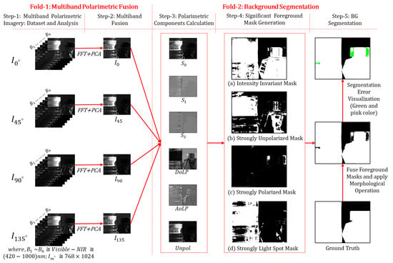
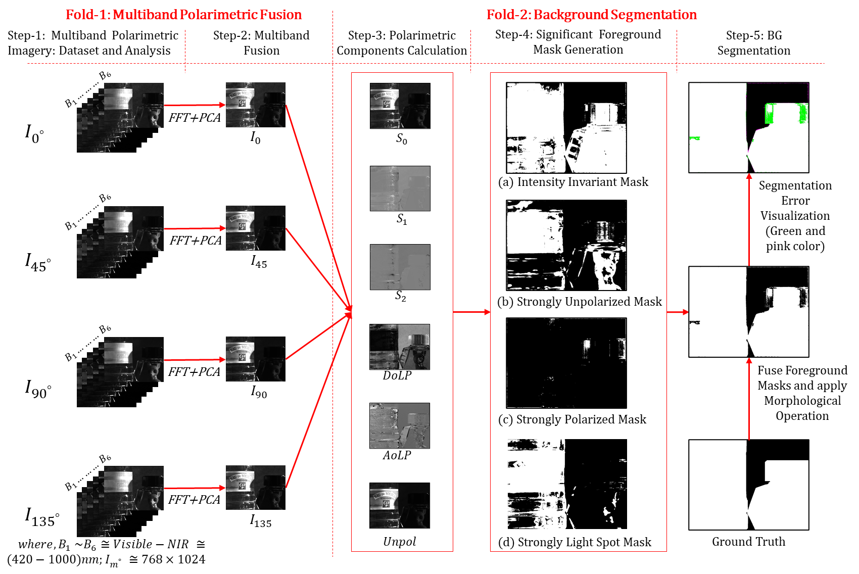
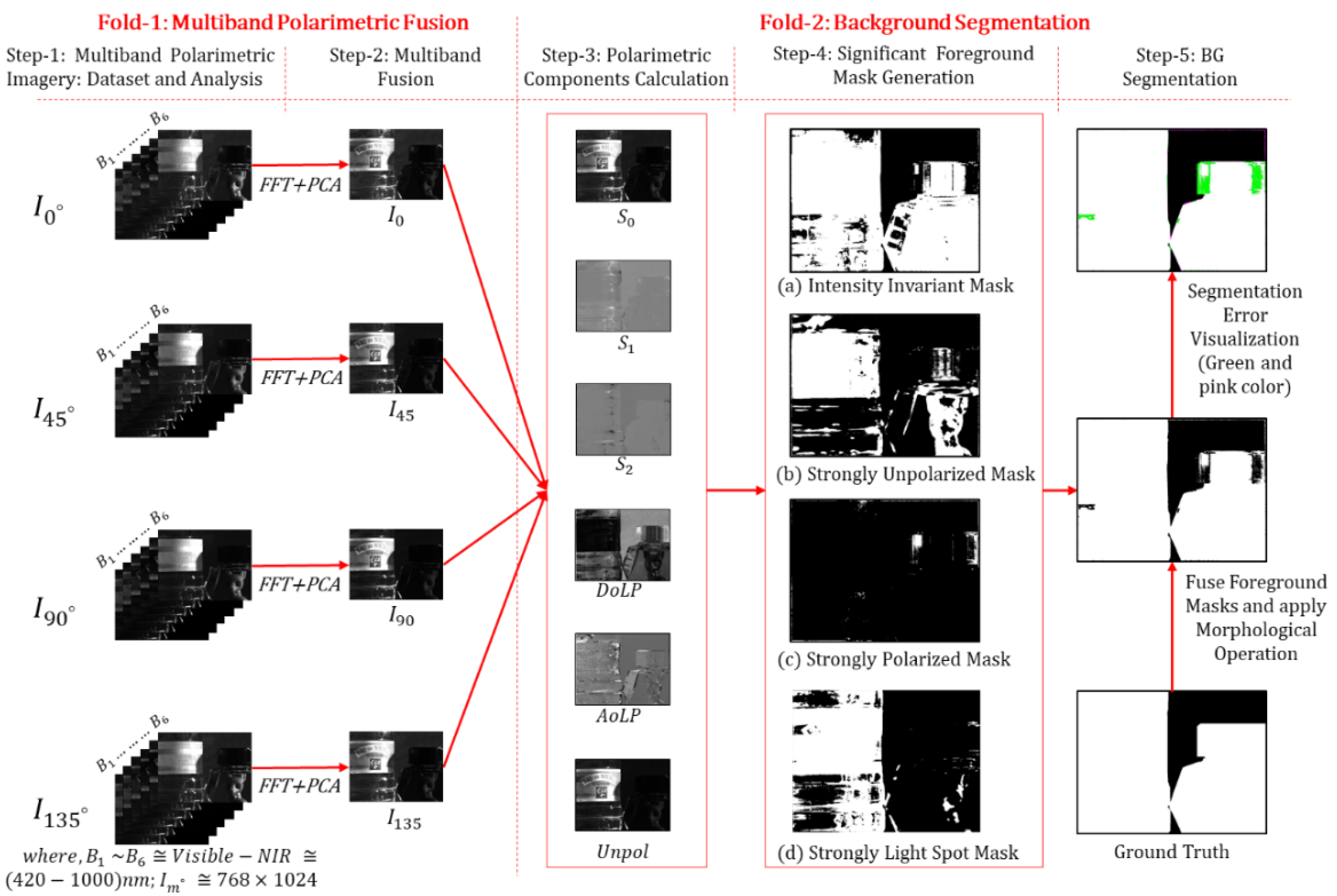
As, in our proposed method, the multiple spectra of each polarimetric filter orientation are fused to solve intricate situations and benefit from the complementarity of the information among multiple bands, it consists of multiband polarimetric fusion and BS. The whole process is decomposed into five main steps: in the first, multiband polarimetric data are captured and analyzed; in the second, a combination of a FFT and PCA is applied on multiple spectra to calculate the fused imagery/image of each polarimetric filter orientation; in the third, the polarimetric components are calculated; in the fourth, four different significant masks are obtained; and, in the last, all of the foreground masks are combined and applied in a morphological operation to generate the final background mask. Figure 5 demonstrates this proposed two-fold BS framework.

The aim of this research is the joint use of spatial, spectral and polarimetric information to segment a polarized background from a complex scene, with Algorithm 1 describing the steps for multiband fusion and BS. In it, the significance of fusion is analyzed by calculating the spectral reflectance, correlation and textural features, and then the proposed fusion algorithm (Algorithm 2) is applied to determine the polarimetric components. Finally, Algorithm 3 is used to segment the background from a complex scene.

Algorithm 1. Multiband Fusion and BS
Requires:
	$Multiband Polarimetric Image Dataset$
Ensures:
	$Background \left(BG\right) segmentation through Multiband Polarimetric Fusion$
1:	Multiband Polarimetric Image Dataset Analysis
2:		Calculate Spectral Reflectance of the Mean Foreground (FG) and BG Area
3:		Calculate Correlation Among Bands and Polarimetric Orientation
4:		Calculate First Order and Second Order Texture Features
5:	ifInformation Differs Significantly among Bands, then
6:		Polarimetric Orientation-wise Multiband Fusion (Algorithm 2)
7:		Evaluate and Performance of the Fusion Method Statistically
8:	end if
9:	if$I_{0^{°}}$, $I_{{45}^{°}}$, $I_{{90}^{°}}$, $I_{{135}^{°}}$exist then
10:		Compute Stokes Vector: $S_0-S_2$
11:		Compute Polarimetric Components:$DoLP$, $AoLP$and$Unpol$
12:	end if
13:	BS in Polarimetric Imagery (Algorithm 3)
14:	Evaluate and Compare Performance of the Proposed Method Statistically

4.2. Hybrid Fusion Framework and Algorithm

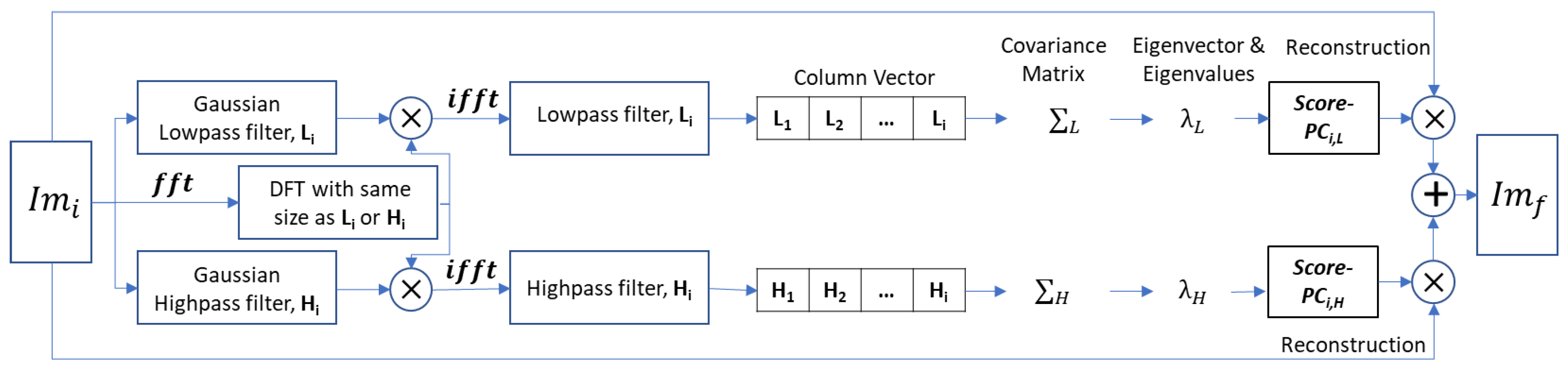
An analysis of MSPI in terms of spectral reflectance, correlation and textural features can predict the significance of multiband pixel-level fusion. The proposed fusion method is based on 2D neighborhood information, such as gradients or edge magnitudes and orientations, with the source images multiple spectral ones ($I{m}_i$) and the fused image ($I{m}_f$) based on different polarimetric filter orientations. This method is hybrid in nature as it combines two different techniques, an FFT and PCA, as shown in Figure 6. Firstly, by applying a Gaussian low-pass filter, each spectral image is decomposed into low- and high-frequency components ($LP{F}_i$ and $HP{F}_i$, respectively). Then, a Discrete Fourier Transform ($DF{T}_i$) of each band is calculated with the help of the FFT. Multiplying the $DF{T}_i$ by the $LP{F}_i$ and $HP{F}_i$, the final FFTs ($FL{P}_i$ and $FH{P}_i$) are obtained. Then, applying an inverse FFT, the results are converted to the spatial domain as the final low and high frequencies of each band as:

$$DF{T}_i=fft\left(ban{d}_i\right)$$

(24)

$$FL{P}_i=LP{F}_i\times DF{T}_i, FH{P}_i=HP{F}_i\times DF{T}_i$$

(25)

$$L{P}_i=ifft\left(FL{P}_i\right), H{P}_i=ifft\left(FH{P}_i\right)$$

(26)

Then, the covariance matrix, eigenvector and eigenvalue of each low- and high-frequency component are calculated and the transformed image reconstructed by determining their first PCs. Finally, these components are combined to obtain the fused image; Figure 6 illustrates the framework of this method. MSPI often presents complementary information about the foreground and background in a scene efficiently combined by pixel-level fusion. The process for polarimetric orientation-wise multiband fused imagery is described in Algorithm 2.

Algorithm 2. Polarimetric Orientation-wise Multiband Fusion
Requires:
	$MSPI Scene Dataset$
Ensures:
	$Polarimetric Orientation-wise Fused Imagery$
1:	forall polarimetric$orientation{s}_k$do
2:		forall$ban{d}_i$do
3:			Create a Gaussian Low Pass Filter ($LP{F}_i$) and Gaussian High Pass Filter ($HP{F}_i$)
4:			Calculate a Discreate Fourier Transform$DF{T}_i$
5:			Multiply$DF{T}_i$with$LP{F}_i$and$HP{F}_i$
6:			Convert the Result to the Spatial Domain by inverting Multiplication result Apply Inverse Fast Fourier Transformation to the multiplication results which produce band-wise final results as$L{P}_{k,i}$and$H{P}_{k,i}$
7:		end for
8:		Calculate the covariance and eigenvector of$L{P}_k$and$H{P}_k$
9:		Calculate the first Principal Component of$L{P}_k$and$H{P}_k$
10:		Calculate the fused imagery by adding both Principal Components
11:	end for

4.3. Calculation of Polarimetric Components

The fused images calculated at different polarimetric orientations ($0^0, {45}^0, {90}^0$, ${135}^0$) are labeled $I_{0^0}$, $I_{{45}^0}$, $I_{{90}^0}$ and $I_{{45}^0}$, respectively, to determine their polarimetric components. The Stokes parameters ($S_0$–$S_2$) [64] describe the linear polarization characteristics using a three-element vector ($S$), as shown in Equation (27), where $S_0$ represents the total intensity of light, $S_1$ the difference between horizontal and vertical polarizations and $S_2$ the difference between linear +45° and −45° ones.

$$S=\left[ \begin{array}{c}{S}_0\\ S_1\\ S_2\end{array} \right]=\left[\begin{array}{c}{I}_{0^0}+I_{{90}^0}\\ I_{0^0}-I_{{90}^0}\\ I_{{45}^0}-I_{{135}^0}\end{array}\right]$$

(27)

The $DoLP$ is a measure of the proportion of the linear polarized light relative to the light’s total intensity, the $AoLP$ the orientation of the major axis of the polarization ellipse, which represents the polarizing angle where the intensity should be the strongest, and the $Unpol$ a measure of the unpolarized light according to the dataset’s author. The $DoLP$, $AoLP$ and $Unpol$ are derived from the Stokes vector, respectively, as:

$$DoLP=\frac{I_{pol}}{I_{tot}}=\frac{\sqrt{S_1^2+S_2^2}}{S_0}$$

(28)

$$AoLP=\frac{1}{2} ta{n}^{-1}\left(\frac{S_2}{S_1}\right)$$

(29)

$$Unpol=S_0-\frac{1}{2}\sqrt{S_1{}^2+S_2{}^2}$$

(30)

4.4. Proposed BS Algorithm

The proposed BS algorithm, which involves five different steps for generating four significant foreground masks through processing the polarimetric components, is presented in Algorithm 3.

Algorithm 3. BS in Polarimetric Imagery
Requires:
	$Stokes Vector and Polarimetric Components$
Ensures:
	$Segmented Background from a scene$
1:	if$S_0-S_2$,$DoLP$,$AoLP$,$UoLP$exist then
2:		Significant Foreground Mask Generation
3:			Construct an intensity invariant mask through differentiating the median filtering version of unpolarized and polarized imagery
4:			Calculate a strongly unpolarized foreground mask in two different ways utilizing$AoLP$and$DoLP$
5:			Calculate a strongly polarized foreground mask
6:			Calculate a strong light intensity mask based on azimuth angle and$S_0$.
7:		Combine steps 3-6 and apply a morphological operation to segment the total background area of a scene.
8:	end if

• Step 1. Construction of intensity-invariant mask

The proportion of the unpolarized to total intensity is defined as the degree of unpolarized intensity (Equation (31)). A $DoLP$ modulation coefficient can be used to stretch the contrast and, thereby, the separability of the foreground/background areas in a polarimetric scene [29]. This function should be continuous in the field of the $DoLP$ and monotonically increase with it. A logarithmic function is a natural choice for this purpose, as pointed out by Shannon [65], and the $DoLP$ modulation coefficient ($M_{DoLP}$) is defined in Equation (32). The differentiation between the median filtering versions of the degree of the unpolarized image ($D_{Unpol}$) and $M_{DoLP}$ in Equation (33) produces an intensity-invariant mask as:

$$D_{Unpol}=Unpol ÷S_0$$

(31)

$$M_{DoLP}=DoLP · log \left(1+DoLP \right)$$

(32)

$$Mas{k}_{IntInv}=\left|D_{Unpol}-M_{DoLP}\right| > Threshold$$

(33)

• Step 2. Construction of strongly unpolarized mask

An indirect unpolarized mask is calculated through a DoLP analysis. Firstly, due to the dark offset and spatial nonuniformity of light, a $DoLP$ image may contain noise. Therefore, a FFT with a Gaussian low-pass filter is applied to smooth it and reduce the noise level (Equation (34), where $D\left(u,v\right)$ is the distance from a point $\left(u,v \right)$ to the center of its frequency in the $DoLP$, and $D_0$ is the cutoff frequency) and the FFT of the $DoLP$ image with padding obtained by Equation (35). The transformed image is multiplied by the filter and then an inverse FFT applied to obtain a noise-free smooth image (Equation (36)). The calculated low-pass filtered image of the $DoLP$ ($Smooth$) is multiplied by the $D_{Unpol}$ to obtain a lower intensity (lower global threshold) of the polarized image and then binarized to calculate a noise-free smooth unpolarized mask (Equation (37)).

$$L\left(u,v\right)=e^{-D^2\left(u,v\right)/2D_0^2}$$

(34)

$$F\left(u,v\right)=fft \left(DoLP\right)$$

(35)

$$S_{DoLP}=ifft \left(L \left(u,v\right)\times F \left(u,v\right)\right)$$

(36)

$$Mas{k}_{IndUnp}=~imbinarize \left(S_{DoLP}\times D_{Unpol} \right)$$

(37)

A direct unpolarized mask is calculated using an $AoLP$ textural analysis. A desultory value of the $AoLP$ denotes a rough surface that indicates the unpolarized part of a scene and a continuous one a smooth surface, which indicates the polarized part of a scene [20]. To segment the unpolarized part, firstly, a textural image is created by applying entropy filtering around a 9-by-9 neighborhood of the $AoLP$. The aim is to obtain an output image ($Mas{k}_{DirUnp}$) in which each output pixel contains the entropy value of the 9-by-9 neighborhood around the corresponding pixel in the input image of the $AoLP$ as:

$$Mas{k}_{DirUnp}=imbinarize \left(entropyfilt\left(AoLP\right)\right)$$

(38)

A final unpolarized mask is generated through a bit-AND operation. Because the contrast, illumination and energy levels are not uniform among the scenes in the bands, some portions of an individual scene gain advantages during this process, with some considering an $AoLP$ textural analysis and others a $DoLP$ one. Applying this operation on both sides obtains an exact unpolarized mask as:

$$Mas{k}_{StUnp}=Mas{k}_{IndUnp} \& Mas{k}_{DirUnp}$$

(39)

• Step 3. Calculation of strongly polarized mask

Based on Otsu’s method for calculating the global threshold, the $DoLP$ image is converted to a binary one to obtain a strongly polarized mask of a scene as:

$$Mas{k}_{StPol}=imbinarize\left(DoLPf\right)$$

(40)

• Step 4. Calculation of strong light intensity mask

The inclination or azimuth angle (β) of the polarized light is calculated. The electric field vector (E) is divided into two orthogonal plane waves ($E_x$ and $E_y$) in the direction of the x- and y-axes, respectively. The calculations of $E_x$ and $E_y$ depend on $S_0, S_1 \mathrm{and} S_2,$ as in Equations (41) and (42), and the azimuth angle is defined in Equation (43). Finally, as the $\beta$ is calculated from the $DoLP$, a noise-free version of it is determined using Equations (41)–(43) and renamed $S_{Azimuth}$.

$$E_x=\sqrt{(S_0\times DoLP)+S_1 }$$

(41)

$$E_y=\sqrt{(S_0\times DoLP)-S_1 }$$

(42)

$$\beta =ta{n}^{-1}\left(E_y/E_x\right)$$

(43)

The total intensity image $(S_0)$ is divided by the logarithmic function of $\beta$ to calculate the area of the maximum strong light intensity. The purpose of using this natural logarithmic function of $\beta$ is to stretch the contrast and, thus, the separability of the strong light intensity areas in polarimetric images by:

$$Mas{k}_{StLight}=imbinarize\left(\frac{S_0}{\log \left(1+S_{Azimuth}\right)}\right)$$

(44)

• Step 5. Combination of foreground masks and application of morphological operation

All the foreground areas, such as the intensity-invariant, strongly unpolarized, strongly polarized and strong light intensity masks, are calculated and fused to obtain the final foreground mask (Equation (45)). Then, a morphological structuring operation based on a dilation followed by an erosion to boost the segmentation performance is applied on the combined background mask. The final background area in the corresponding scene is denoted in black and it can be seen that some object parts are mixed with the background due to the presence of polarization.

$$Mas{k}_{Foreground}=Mas{k}_{IntInv} \cup Mas{k}_{StUnp}\cup Mas{k}_{StPol} \cup Mas{k}_{StLight}$$

(45)

5. Experimental Results

In this section, performance evaluations and comparisons of the proposed two-fold BS and other approaches using different metrics in terms of multiband fusion and polarimetric BS are discussed. Also, computational time analyses of individual methods are conducted.

5.1. Performance Evaluation of MSPI Fusion

5.1.1. Selection of Fusion Metric

Currently, the quality of a fused image can be quantitively evaluated using the metrics [66] Mean Absolute Percentage Error (MAPE), Peak Signal-to-Noise Ratio (PSNR), Pearson Correlation Coefficient (PCOR) and Mutual Information (MI). The MAPE is a measure of the closeness between predictions of the reference and fused images. The PSNR block computes the PSNRs of the reference and fused images. A lower value of MAPE and higher value of PSNR indicate a better quality of the reconstructed or fused image. The PCOR computes the linear correlation coefficient between the reference and fused images, while MI indicates the mutual dependence between them, with the higher their values, the better the correlation. Considering two images $A$ and $B$, the mathematical evaluation measures of the aforementioned metrics are:

$$MAPE=\frac{1}{n} {\displaystyle \sum }_{i=1}^n\left|\left(\frac{A_i-B_i}{B_i}\right)\times 100\right|$$

(46)

$$PSNR=10 . lo{g}_{10} \left(\frac{MA{X}_I^2}{MSE}\right)$$

(47)

$$PCOR=\frac{{{\displaystyle \sum }}_m{{\displaystyle \sum }}_n\left(A_{mn}-\overline{A}\right) \left(B_{mn}-\overline{B}\right)}{\sqrt{({{\displaystyle \sum }}_m{{\displaystyle \sum }}_n{\left(A_{mn}-\overline{A}\right)}^2) ({{\displaystyle \sum }}_m{{\displaystyle \sum }}_n{\left(B_{mn}-\overline{B}\right)}^2)} }$$

(48)

$$MI={\displaystyle \sum }_{a\in A}{\displaystyle \sum }_{b\in B}P\left(a,b\right)\log \frac{P\left(a,b\right)}{P\left(a\right) P\left(b\right)}$$

(49)

5.1.2. Observation of Fusion Quality

To evaluate the performance of fusion, the median image of each band is considered the reference one and the fused image the resultant one. The former contains the central value of the bands and tends to retain more detailed information.

Table 1. Mean Absolute Percentage Error and Peak Signal-to-Noise Ratio error metrics (MAPE, PSNR) and Pearson Correlation Coefficient and Mutual Information correlation metrics (PCOR, MI) of different fusion methods.

		MAPE				PSNR				PCOR				MI
		0°	45°	90°	135°	0°	45°	90°	135°	0°	45°	90°	135°	0°	45°	90°	135°
Liquid Scene	DWT [37]	26.28	33.42	41.25	31.74	31.94	32.96	31.73	32.28	0.99	0.99	0.99	0.98	2.32	2.42	2.32	2.18
	PCA [33]	19.23	26.47	34.69	22.54	29.05	28.88	28.86	28.86	0.99	0.99	0.99	0.99	2.62	2.72	2.64	2.49
	DCT–LP [40]	146.25	167.14	189.36	150.89	23.19	24.57	24.12	22.99	0.81	0.83	0.84	0.82	0.93	1.09	1.01	0.92
	SHT [20]	93.80	123.43	164.35	116.91	19.60	19.32	20.01	19.46	0.86	0.88	0.88	0.86	1.32	1.48	1.37	1.25
	FPDE [34]	16.79	21.53	27.83	19.28	30.48	31.08	31.24	30.51	0.99	0.99	0.99	0.99	2.73	2.87	2.77	2.63
	Proposed	30.86	39.55	52.80	35.23	18.90	19.37	19.49	19.10	0.99	0.99	0.99	0.99	2.89	2.97	2.84	2.75
Food Scene	DWT [37]	11.13	16.33	15.08	14.22	32.56	32.28	31.37	32.04	0.99	0.99	0.99	0.99	2.68	2.60	2.57	2.76
	PCA [33]	5.06	8.81	8.56	6.64	30.19	28.13	27.53	30.00	0.99	0.99	0.98	0.99	3.02	2.76	2.68	3.00
	DCT–LP [40]	93.21	156.36	157.00	122.33	21.64	21.59	21.24	22.05	0.84	0.81	0.81	0.83	1.17	1.04	1.02	1.16
	SHT [20]	20.39	30.40	30.56	22.83	20.47	19.21	18.38	20.01	0.95	0.92	0.92	0.94	1.87	1.70	1.62	1.85
	FPDE [34]	19.79	31.96	30.23	25.02	20.11	18.76	19.16	19.93	0.90	0.80	0.81	0.89	2.21	1.77	1.77	2.20
	Proposed	10.14	15.66	15.08	12.22	16.90	18.15	18.32	17.14	1.00	0.99	0.99	1.00	3.32	3.07	3.05	3.43
Leaf Scene	DWT [37]	15.00	14.45	14.52	14.95	26.14	26.63	26.60	26.29	0.98	0.97	0.97	0.98	2.20	2.07	2.07	2.22
	PCA [33]	5.32	8.64	9.51	5.37	26.95	22.53	21.97	26.60	0.99	0.94	0.93	0.99	2.78	2.35	2.30	2.75
	DCT–LP [40]	55.15	63.95	62.89	54.54	14.87	14.53	14.61	14.82	0.84	0.76	0.75	0.84	1.17	1.10	1.12	1.18
	SHT [20]	26.72	32.41	36.56	26.46	13.19	11.96	11.89	13.04	0.86	0.76	0.74	0.85	1.58	1.57	1.56	1.60
	FPDE [34]	9.51	24.55	32.66	10.82	25.41	20.43	18.84	24.64	0.98	0.89	0.86	0.97	3.43	2.01	1.48	3.28
	Proposed	10.41	14.39	15.58	10.30	10.54	12.14	12.22	10.75	0.99	0.96	0.95	0.99	2.89	2.52	2.47	2.88
Average	DWT [37]	17.47	21.40	23.62	20.30	30.21	30.63	29.90	30.20	0.99	0.98	0.98	0.99	2.40	2.36	2.32	2.39
	PCA [33]	9.87	14.64	17.59	11.52	28.73	26.51	26.12	28.49	0.99	0.97	0.97	0.99	2.81	2.61	2.54	2.74
	DCT–LP [40]	98.20	129.15	136.42	109.25	19.90	20.23	19.99	19.95	0.83	0.80	0.80	0.83	1.09	1.08	1.05	1.09
	SHT [20]	46.97	62.08	77.16	55.40	17.75	16.83	16.76	17.50	0.89	0.85	0.85	0.88	1.59	1.58	1.52	1.57
	FPDE [34]	15.36	26.01	30.24	18.37	25.33	23.42	23.08	25.03	0.95	0.89	0.88	0.95	2.79	2.22	2.01	2.70
	Proposed	17.14	23.20	27.82	19.25	15.44	16.55	16.68	15.66	0.99	0.98	0.98	0.99	3.03	2.86	2.79	3.02

demonstrates that the average PSNR value of the proposed method is lower than other methods; however, the average MAPE value is significantly better than some references. The average metric value of the three scenes demonstrates that the fusion quality of our proposed hybrid fusion-based approach is superior in terms of its higher PCOR and MI compared to those in the current literature.

5.1.3. Comparison of Performances of Fusion Methods

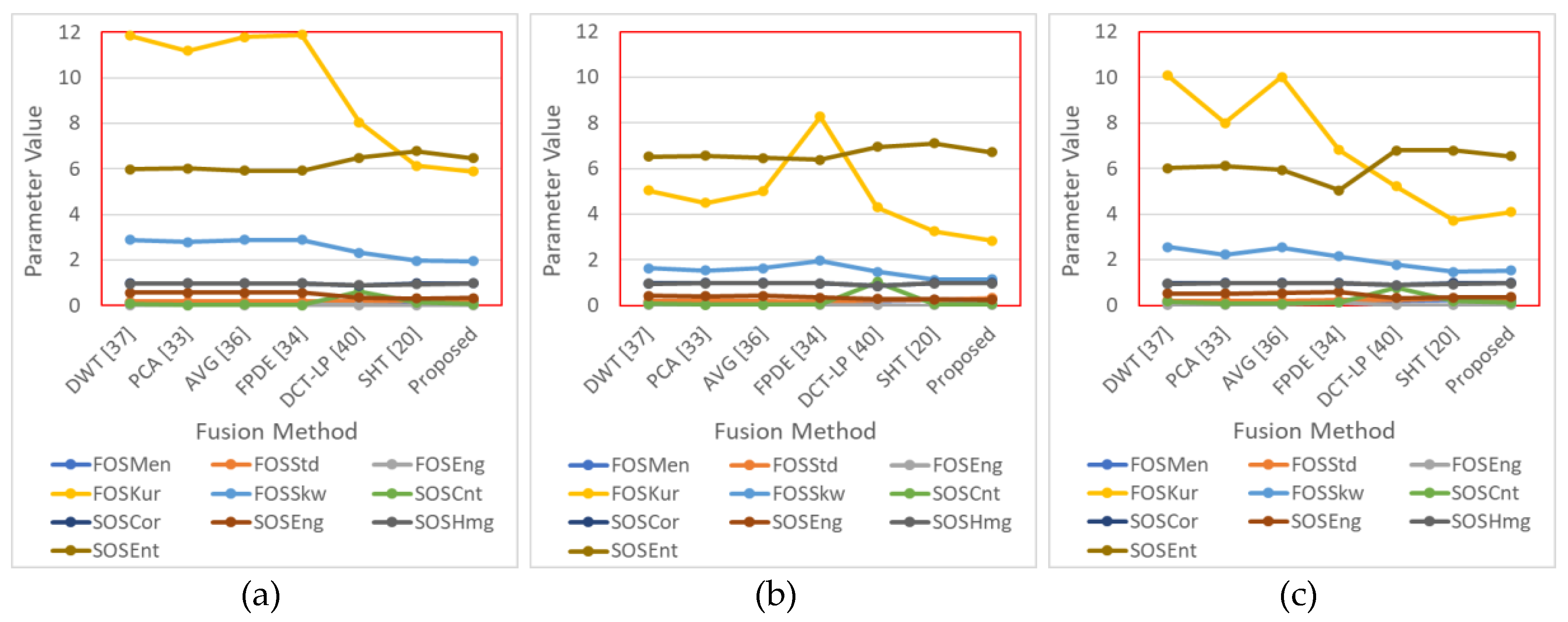
The textural features of the fused images are presented in Figure 7. It can be seen that the kurtosis, skewness and energy of the liquid, food and leaf scenes demonstrate lower values for the proposed hybrid fusion method than for the DWT [37], PCA [33], AVG [36], DCT–LP [40], SHT [20] and FDPE [34] while, in contrast, its entropy is predicted to be higher than those of the DWT, PCA and AVG methods. Therefore, it is considered that, overall, the proposed hybrid pixel-level fusion method generates the maximum amount of information among multiple spectra.

5.1.4. Visualization of Fusion Performance

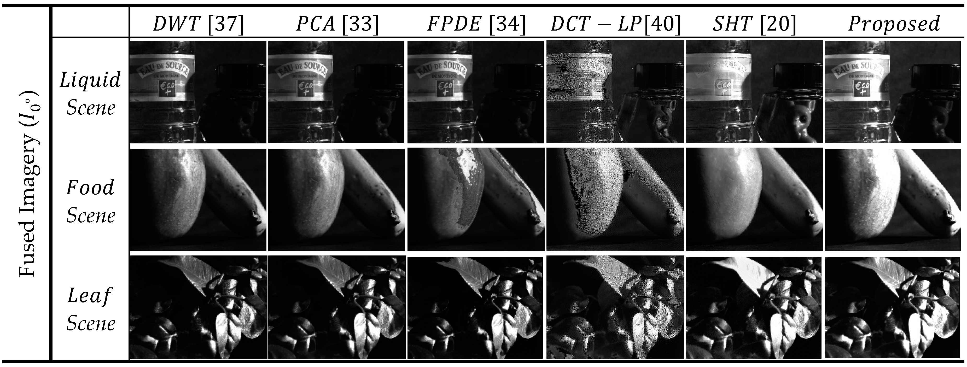
It is obvious that multiband fusion methods demonstrate better BS accuracy than direct processing [67,68]. The multiband fusion results shown in Figure 8 demonstrate that the proposed hybrid fusion approach has an advantage over the other methods as it appears strongly at the edge of an object, which will enable foreground objects to be further separated from a scene.

5.2. Calculation of Polarimetric Component

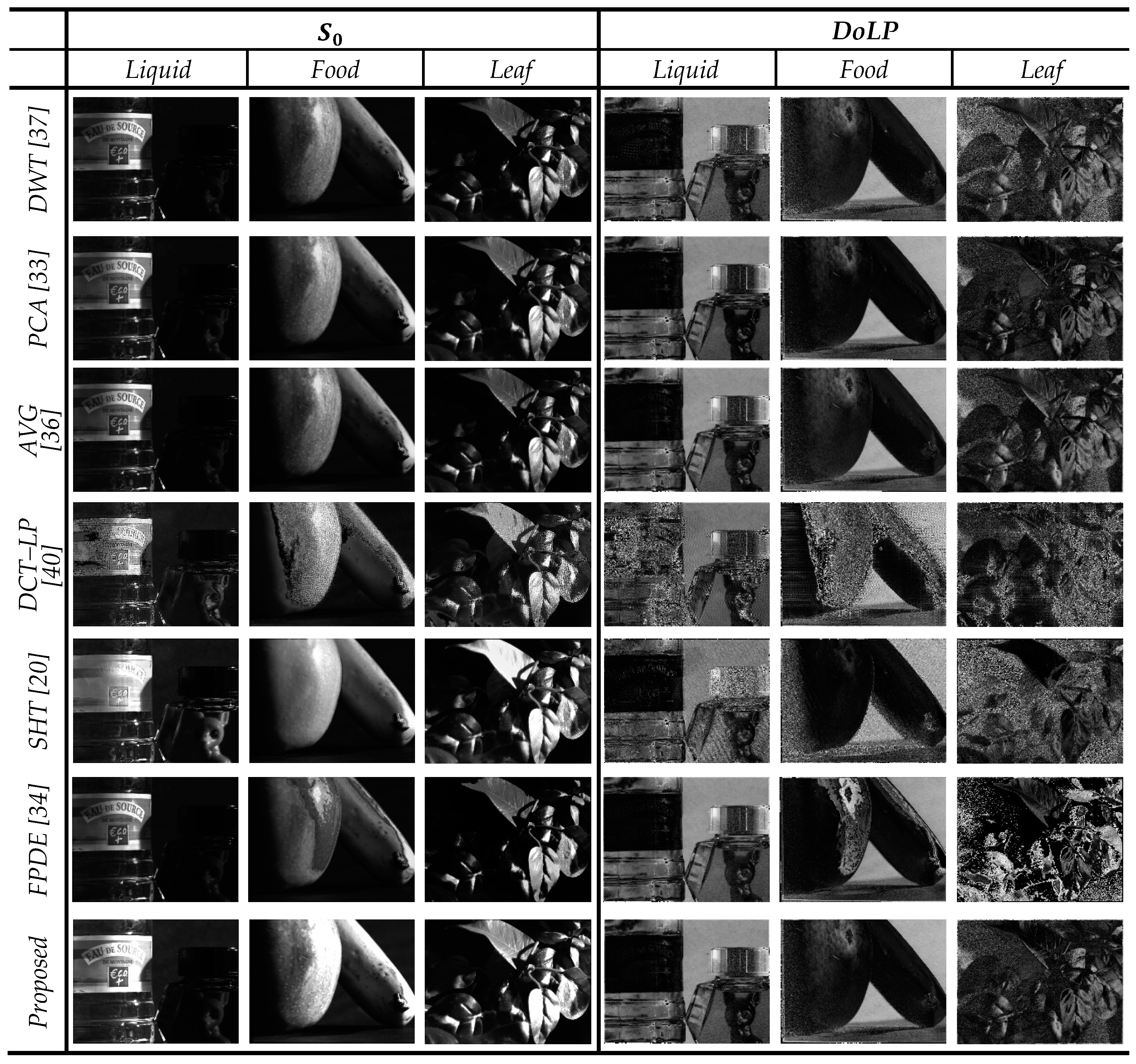
Based on different fusion methods, the polarimetric components $S_0$ and $DoLP$ are calculated and shown in Figure 9. Analyzing the $DoLP$ values, it is predicted that, in the scenes, the backgrounds are polarized, whereas the foregrounds have mixed polarized and unpolarized intensities.

5.3. Performance Evaluation of MSPI BS

5.3.1. Selection of BS Metric

The BS method is evaluated at the pixel level of a binarized scene in which the foreground and background are white and black, respectively. Its performance can be divided into four pixel-wise classification results: true positives ($T_p$), which mean correctly detected foreground pixels; false positives ($F_p$), that is, background pixels incorrectly detected as foreground ones; true negatives ($T_n$), which indicate correctly detected background pixels; and false negatives ($F_n$), that is, foreground pixels incorrectly detected as background ones. The binary classification metrics used in this paper are accuracy, specificity, sensitivity, Geometric mean (G-mean), precision, recall and the F1-score. Accuracy is measured as the proportion of true results obtained, either $T_n$ or $T_p$; specificity (a $T_n$ fraction) as the proportion of actual negatives predicted as negatives; sensitivity (a $T_p$ fraction) as the proportion of actual positives predicted as positives; the G-mean, the root of the product of specificity and sensitivity; precision, the number of foreground pixels detected that are actually foreground ones; recall, the number of foreground pixels detected from the actual foreground (recall and sensitivity are similar); the F1-score (a boundary F1 measure) the harmonic mean of the precision and recall values, which measures how closely the predicted boundary of an object matches its ground-truth and is an overall indicator of the performance of binary segmentation. The mathematical evaluation measures of the aforementioned metrics follow [69]:

$$Accuracy \left(AC\right)=\frac{T_p+T_n}{T_p+F_n+T_n+F_p}$$

(50)

$$Specificity \left(SP\right)=\frac{T_n}{T_n+F_p}$$

(51)

$$Sensitivity \left(SN\right) or Recall \left(RC\right)=\frac{T_p}{T_p+F_n}$$

(52)

$$Geometric-Mean \left(GM\right)=\sqrt{Specificity\times Sensitivity}$$

(53)

$$Precision \left(PR\right)=\frac{T_p}{T_p+F_p}$$

(54)

$$F1-Score \left(F1S\right)= 2\times \frac{Precision\times Recall}{Precision+Recall}$$

(55)

5.3.2. Generation of Ground Truth

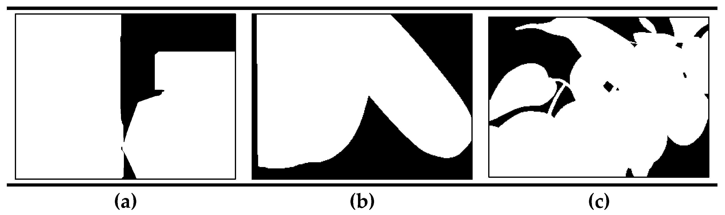
Each ground truth is generated manually by an expert with the maximum possible background among bands covered. In Figure 10, for the scenes’ binary ground truths, the black and white pixels indicate their backgrounds and foregrounds, respectively.

5.3.3. Comparison of BS Accuracy: Direct vs. Fusion

In

Table 2. Evaluation of direct- vs. fusion-based BS performances for three scenes in the MSPI dataset.

	Direct BG Separation								Fusion-based BG Segmentation
		AC	SP	SN	GM	PR	RC	F1S		AC	SP	SN	GM	PR	RC	F1S
Liquid Scene	B-1	0.91	0.68	0.96	0.80	0.93	0.96	0.94	DWT [37]	0.96	0.97	0.96	0.97	0.99	0.96	0.98
	B-2	0.91	0.74	0.95	0.84	0.94	0.95	0.95	PCA [33]	0.96	0.95	0.96	0.95	0.99	0.96	0.97
	B-3	0.92	0.84	0.94	0.89	0.96	0.94	0.95	AVG [36]	0.96	0.98	0.95	0.97	1.00	0.95	0.97
	B-4	0.91	0.61	0.98	0.77	0.92	0.98	0.95	DCT–LP [40]	0.94	0.73	0.98	0.85	0.94	0.98	0.96
	B-5	0.91	0.78	0.94	0.86	0.95	0.94	0.94	SHT [20]	0.95	0.81	0.98	0.89	0.96	0.98	0.97
	B-6	0.95	0.81	0.98	0.89	0.96	0.98	0.97	FPDE [34]	0.92	0.98	0.91	0.94	1.00	0.91	0.95
									Proposed	0.97	0.98	0.97	0.97	1.00	0.97	0.98
Food Scene	B-1	0.62	0.69	0.59	0.64	0.81	0.59	0.68	DWT [37]	0.91	0.85	0.93	0.89	0.93	0.93	0.93
	B-2	0.59	0.76	0.51	0.63	0.83	0.51	0.63	PCA [33]	0.95	0.85	0.99	0.92	0.94	0.99	0.96
	B-3	0.54	0.88	0.39	0.59	0.88	0.39	0.54	AVG [36]	0.92	0.87	0.94	0.90	0.94	0.94	0.94
	B-4	0.60	0.67	0.56	0.61	0.79	0.56	0.66	DCT–LP [40]	0.92	0.75	0.99	0.86	0.90	0.99	0.94
	B-5	0.53	0.87	0.37	0.57	0.86	0.37	0.52	SHT [20]	0.85	0.73	0.91	0.82	0.88	0.91	0.89
	B-6	0.93	0.80	0.99	0.89	0.92	0.99	0.95	FPDE [34]	0.84	0.79	0.86	0.82	0.90	0.86	0.88
									Proposed	0.96	0.90	0.99	0.94	0.96	0.99	0.97
Leaf Scene	B-1	0.65	0.25	0.77	0.44	0.77	0.77	0.77	DWT [37]	0.71	0.90	0.65	0.76	0.95	0.65	0.77
	B-2	0.63	0.29	0.73	0.46	0.77	0.73	0.75	PCA [33]	0.80	0.82	0.79	0.80	0.93	0.79	0.86
	B-3	0.67	0.63	0.68	0.66	0.86	0.68	0.76	AVG [36]	0.81	0.80	0.82	0.81	0.93	0.82	0.87
	B-4	0.68	0.24	0.81	0.44	0.78	0.81	0.79	DCT–LP [40]	0.92	0.81	0.95	0.88	0.94	0.95	0.94
	B-5	0.55	0.52	0.57	0.54	0.79	0.57	0.66	SHT [20]	0.76	0.55	0.82	0.67	0.86	0.82	0.84
	B-6	0.82	0.26	1.00	0.50	0.81	1.00	0.89	FPDE [34]	0.58	0.83	0.50	0.65	0.91	0.50	0.65
									Proposed	0.89	0.84	0.90	0.87	0.95	0.90	0.92
Average	Direct	0.74	0.63	0.76	0.67	0.86	0.76	0.80	Fusion	0.88	0.84	0.89	0.86	0.94	0.89	0.91

, the performances of BS in terms of the metrics for direct and fusion-based approaches are compared, where B-1 to B-6 denote Bands 1 to 6, respectively, in the range of 400–1000 nm. As can be seen, the mean of an individual evaluation metric is significantly higher for a fusion-based BS method than for a direct band-wise BS one. Also, it can be ascertained that the mean accuracy, G-mean and F1-score are 0.88, 0.86 and 0.91, respectively, for the former, and 0.74, 0.67 and 0.80 for the latter.

5.3.4. Visualization of Performance of BS

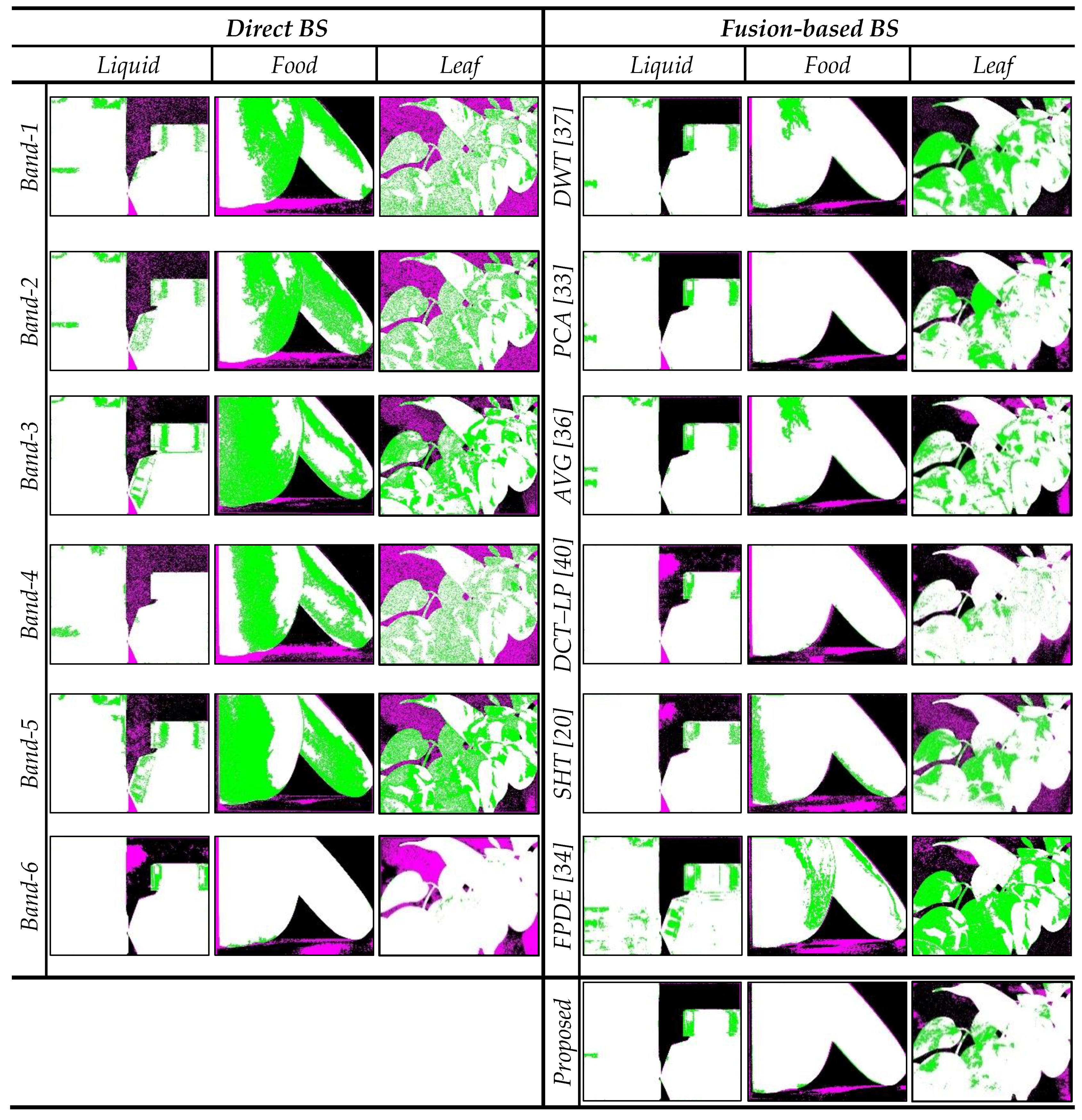
The polarimetric BS errors are shown in Figure 11 in which purple and green denote the error areas of the segmentation methods present in the ground truths’ black and white portions, respectively. These errors are lower for the fusion-based methods than for the direct band-wise ones, with our proposed hybrid fusion-based polarimetric BS approach superior to all the others.

5.3.5. Comparison of BS Accuracy: Proposed Method vs. Those in Literature

It is worth mentioning that the performances of these existing BS methods are not exactly comparable, as each reports its accuracy for a specific MSPI database. Also, the recognition accuracy values obtained from the fusion methods and color-mapping techniques used for segmentation vary.

By integrating an FFT with PCA for a fusion approach and then generating foreground masks for the segmentation task, the proposed BS method obtains higher accuracy, G-mean and F1-score values for the liquid (0.97, 0.97 and 0.98, respectively), food (0.96, 0.94 and 0.97, respectively) and leaf (0.89, 0.87 and 0.92, respectively) scenes in the MSPI dataset than those in the existing literature on foreground separation methods, as presented in

Table 3. Comparison of performances of BS methods for three scenes in the MSPI dataset.

	Liquid Scene							Food Scene							Leaf Scene
	AC	SP	SN	GM	PR	RC	F1S	AC	SP	SN	GM	PR	RC	F1S	AC	SP	SN	GM	PR	RC	F1S
Wolf [13]	0.69	0.00	0.84	0.06	0.79	0.84	0.82	0.57	0.99	0.38	0.61	0.99	0.38	0.55	0.65	0.40	0.73	0.54	0.80	0.73	0.76
Zhao [29]	0.95	1.00	0.94	0.97	1.00	0.94	0.97	0.81	0.38	1.00	0.62	0.78	1.00	0.88	0.44	0.93	0.28	0.51	0.93	0.28	0.44
Zhou [20]	0.67	1.00	0.60	0.78	1.00	0.60	0.75	0.70	0.85	0.62	0.73	0.90	0.62	0.74	0.58	0.40	0.64	0.51	0.78	0.64	0.70
Lu [59]	0.75	1.00	0.69	0.83	1.00	0.69	0.82	0.89	0.72	0.96	0.83	0.88	0.96	0.92	0.51	0.62	0.48	0.54	0.80	0.48	0.60
Proposed	0.97	0.98	0.97	0.97	1.00	0.97	0.98	0.96	0.90	0.99	0.94	0.96	0.99	0.97	0.89	0.84	0.90	0.87	0.95	0.90	0.92

.

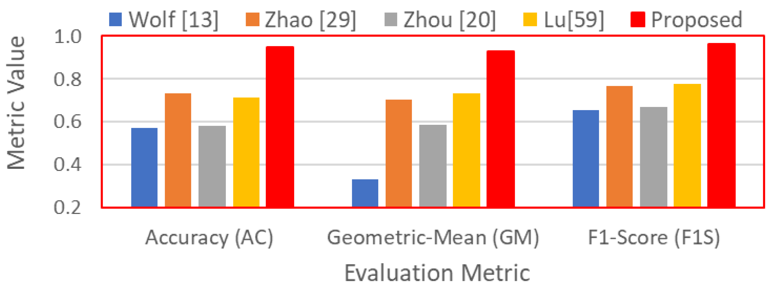
Figure 12 shows the average performances of individual methods for scenes in the MSPI dataset. It is clear that the proposed method performs better than the others with a mean accuracy, G-mean and F1-score of 0.95, 0.93 and 0.97, respectively.

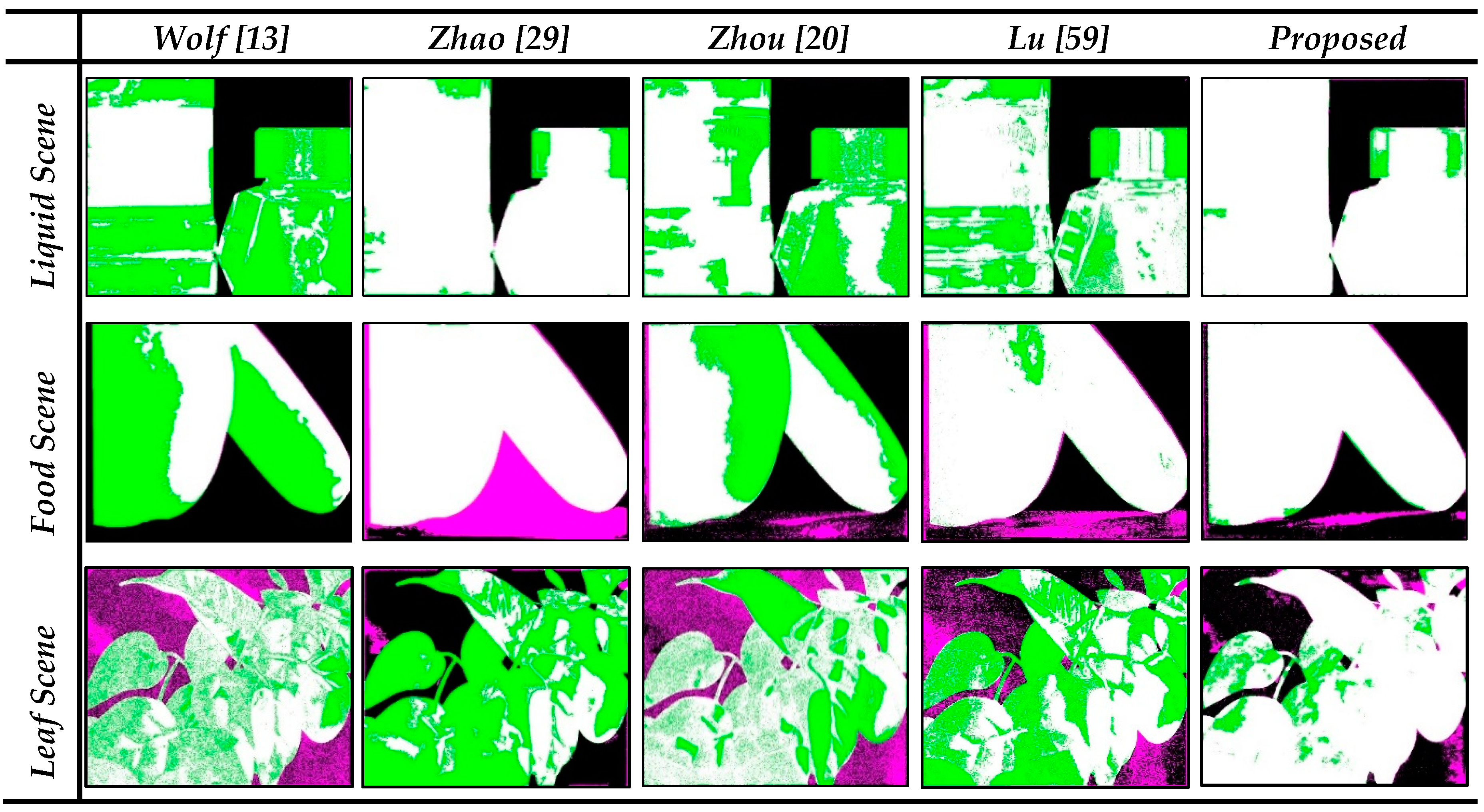
Figure 13 presents the error areas (purple and green) obtained from the individual methods for different scenes in the MSPI dataset. As can be seen, the proposed system reports fewer BS errors than the others. In the liquid scene, however, the background is completely separated by the proposed method, due to weak polarization in the jar cap’s area; it has some errors. In the food (apple and banana) and leaf scenes, although their foregrounds are completely separated by the proposed method, there are some errors due to strong unpolarization in their background areas.

5.4. Computational Time Analysis

The experiments are carried out using MATLAB on a desktop with a hardware configuration of 16 GB RAM and 3.4 GHz Intel Core i7 CPU.

Table 4. Analysis of computational times of different techniques for three scenes in the MSPI dataset.

Running Time (Seconds) – Multiband Fusion					Running Time (Seconds) – Polarimetric BS
	Liquid	Food	Leaf	Average		Liquid	Food	Leaf	Average
DWT [37]	55.76	57.01	57.51	56.76	Wolf [13]	10.74	10.14	11.35	10.74
PCA [33]	38.70	38.19	37.26	38.05	Zhao [29]	8.66	8.93	7.40	8.33
AVG [36]	63.05	63.47	62.94	63.15	Zhou [20]	12.38	8.95	12.57	11.30
DCT–LP [40]	56.40	56.00	56.70	56.37	Lu [59]	10.81	10.61	11.60	11.01
SHT [20]	162.06	163.48	160.23	161.92	Proposed	2.52	3.45	3.74	3.23
FPDE [34]	113.20	113.91	113.90	113.67
Proposed	44.65	44.62	44.58	44.62

presents the running times (in seconds) of the individual methods for multiband fusion and polarimetric BS approach. As can be seen, the proposed system incurs slightly longer computational times than the PCA-based multiband fusion method, but shorter ones than the polarimetric BS, with its shortest mean running time demonstrating its effectiveness in terms of BS in MSPI.

6. Conclusions

In this paper, a two-fold BS approach involving multiband fusion followed by polarimetric BS is proposed for MSPI. Combining complementary information from spectral and polarimetric cues in the visible and NIR ranges improves a foreground’s contrast and details. This framework and algorithm demonstrate the significance of multiband fusion through analyzing spectral reflectance, correlation and textural features. The proposed hybrid fusion method first decomposes each band image into low and high frequencies using an FFT. Then a PCA is performed, with the first PC of each frequency computed and combined with the others to obtain a final fused image. The proposed fusion algorithm predicts better fusion quality with fewer errors in terms of the MAPE, PSNR, COR and MI than the DWT, PCA, DCT–LP, SHT and FPDE techniques. After fusion, the polarimetric components are calculated through a Stokes vector analysis. Finally, four significant foreground masks are generated and combined with the polarimetric components to segment the complex background of a scene. The proposed BS algorithm is compared with four baseline approaches based on fusion, color mapping and fuzzy C-means clustering using an MSPI dataset. The experimental results illustrate the validity and efficiency of the proposed BS method based on diverse performance evaluation metrics. They also demonstrate that it significantly improves the mean accuracy, G-mean and F1-score to 0.95, 0.93, 0.97, respectively, for three scenes in the MSPI dataset compared with those in the existing literature referenced in this paper.

As an extension of this work, we will investigate an advanced BS method in which the background and foreground of a scene are mixed with polarized and unpolarized intensities. We will also address the issues related to the specular reflection of the foreground area in a scene that may mistakenly be detected as the background. As it is known that the specular reflection in an area of strong light intensity can destroy the shape of an actual object; developing an algorithm for detecting and reconstructing a secular reflection in the MSPI dataset will be explored.

References

- Lapray, P.J.; Gendre, L.; Foulonneau, A.; Bigué, L. Database of polarimetric and multispectral images in the visible and NIR regions. In Unconventional Optical Imaging, Proceedings of the SPIE, Strasbourg, France, 24 May 2018; SPIE: Bellingham, WA, USA, 2018. [Google Scholar]
- Yan, Q.; Shen, X.; Xu, L.; Zhuo, S.; Zhang, X.; Shen, L.; Jia, J. Crossfield joint image restoration via scale map. In Proceedings of the IEEE International Conference on Computer Vision, Sydney, NSW, Australia, 1–8 December 2013. [Google Scholar]
- Schaul, L.; Fredembach, C.; Susstrunk, S. Color image dehazing using the near-infrared. In Proceedings of the 16th IEEE International Conference on Image Processing (ICIP), Chiang Mai, Thailand, 7 November 2009. [Google Scholar]
- Salamati, N.; Larlus, D.; Csurka, G.; Süsstrunk, S. Semantic image segmentation using visible and near-infrared channels. In Proceedings of the European Conference on Computer Vision, Florence, Italy, 7–13 October 2012. [Google Scholar]
- Berns, R.S.; Imai, F.H.; Burns, P.D.; Tzeng, D.Y. Multispectral-based color reproduction research at the Munsell Color Science Laboratory. In Electronic Imaging: Processing, Printing, and Publishing in Color, Proceedings of the SPIE, Zurich, Switzerland, 7 September 1998; SPIE: Bellingham, WA, USA, 1998. [Google Scholar]
- Thomas, J.B. Illuminant estimation from uncalibrated multispectral images. In Proceedings of the 2015 Colour and Visual Computing Symposium (CVCS), Gjovik, Norway, 25–26 August 2015. [Google Scholar]
- Motohka, T.; Nasahara, K.N.; Oguma, H.; Tsuchida, S. Applicability of green-red vegetation index for remote sensing of vegetation phenology. Remote Sens. 2010, 2, 2369–2387. [Google Scholar]
- Dandois, J.P.; Ellis, E.C. Remote sensing of vegetation structure using computer vision. Remote. Sens. 2010, 2, 1157–1176. [Google Scholar] [CrossRef] [Green Version]
- Rfenacht, D.; Fredembach, C.; Süsstrunk, S. Automatic and accurate shadow detection using near-infrared information. IEEE Trans. Pattern Anal. Mach. Intell. 2014, 36, 1672–1678. [Google Scholar] [CrossRef] [PubMed]
- Sobral, A.; Javed, S.; Ki Jung, S.; Bouwmans, T.; Zahzah, E.H. Online stochastic tensor decomposition for background subtraction in multispectral video sequences. In Proceedings of the 2015 IEEE International Conference on Computer Vision Workshop (ICCVW), Santiago, Chile, 7–13 December 2015. [Google Scholar]
- Tyo, J.S.; Goldstein, D.L.; Chenault, D.B.; Shaw, J.A. Review of passive imaging polarimetry for remote sensing applications. Appl. Opt. 2006, 45, 5453–5469. [Google Scholar] [CrossRef] [PubMed] [Green Version]
- Nayar, S.K.; Fang, X.-S.; Boult, T. Separation of reflection components using color and polarization. Int. J. Comput. Vis. 1997, 21, 163–186. [Google Scholar] [CrossRef]
- Wolff, L.B. Polarization-based material classification from specular reflection. IEEE Trans. Pattern Anal. Mach. Intell. 1990, 12, 1059–1071. [Google Scholar] [CrossRef]
- Atkinson, G.A.; Hancock, E.R. Shape estimation using polarization and shading from two views. IEEE Trans. Pattern Anal. Mach. Intell. 2007, 29, 2001–2017. [Google Scholar]
- Tan, J.; Zhang, J.; Zhang, Y. Target detection for polarized hyperspectral images based on tensor decomposition. IEEE Geosci. Remote Sens. Lett. 2017, 14, 674–678. [Google Scholar] [CrossRef]
- Goudail, F.; Terrier, P.; Takakura, Y.; Bigue, L.; Galland, F.; DeVlaminck, V. Target detection with a liquid-crystal-based passive stokes polarimeter. Appl. Opt. 2004, 43, 274–282. [Google Scholar] [CrossRef] [Green Version]
- Denes, L.J.; Gottlieb, M.S.; Kaminsky, B.; Huber, D.F. Spectropolarimetric imaging for object recognition. In Proceedings of the 26th AIPR Workshop: Exploiting New Image Sources and Sensors, Washington, DC, USA, 1 March 1998. [Google Scholar]
- Romano, J.M.; Rosario, D.; McCarthy, J. Day/night polarimetric anomaly detection using SPICE imagery. IEEE Trans. Geosci. Remote Sens. 2012, 50, 5014–5023. [Google Scholar] [CrossRef]
- Islam, M.N.; Tahtali, M.; Pickering, M. Man-made object separation using polarimetric imagery. In Proceedings of the SPIE Future Sensing Technologies, Tokyo, Japan, 12–14 November 2019. [Google Scholar]
- Zhou, P.C.; Liu, C.C. Camouflaged target separation by spectral-polarimetric imagery fusion with shearlet transform and clustering segmentation. In Proceedings of the International Symposium on Photoelectronic Detection and Imaging 2013: Imaging Sensors and Applications, Beijing, China, 21 August 2013. [Google Scholar]
- Domadiya, P.; Shah, P.; Mitra, S.K. Fast and Accurate Foreground Background Separation for Video Surveillance. In Proceedings of the 6th International Conference on Pattern Recognition and Machine Intelligence (PReMI), Warsaw, Poland, 30 June–3 July 2015; Springer: Cham, Switzerland, 2015. [Google Scholar]
- Bouwmans, T. Traditional and recent approaches in background modeling for foreground detection: An overview. Comput. Sci. Rev. 2014, 11, 31–66. [Google Scholar] [CrossRef]
- Perazzi, F.; Pont-Tuset, J.; McWilliams, B.; Van Gool, L.; Gross, M.; Sorkine-Hornung, A. A benchmark dataset and evaluation methodology for video object segmentation. In Proceedings of the 2016 IEEE Conference on Computer Vision and Pattern Recognition (CVPR), Las Vegas, NV, USA, 27–30 June 2016. [Google Scholar]
- Zitova, B.; Flusser, J. Image registration methods: A survey. Image Vis. Comput. 2003, 21, 977–1000. [Google Scholar] [CrossRef] [Green Version]
- Benezeth, Y.; Sidibé, D.; Thomas, J.B. Background subtraction with multispectral video sequences. In Proceedings of the IEEE International Conference on Robotics and Automation workshop on Nonclassical Cameras, Camera Networks and Omnidirectional Vision (OMNIVIS), Hong Kong, China, 11 June 2014. HAL-00986168f. [Google Scholar]
- Ma, J.; Ma, Y.; Li, C. Infrared and visible image fusion methods and applications: A survey. Inf. Fusion 2019, 45, 153–178. [Google Scholar] [CrossRef]
- Zhan, L.; Zhuang, Y.; Huang, L. Infrared and visible images fusion method based on discrete wavelet transform. J. Comput. 2017, 28, 57–71. [Google Scholar] [CrossRef]
- Li, H.; Liu, L.; Huang, W.; Yue, C. An improved fusion algorithm for infrared and visible images based on multi-scale transform. Infrared Phys. Technol. 2016, 74, 28–37. [Google Scholar] [CrossRef]
- Zhao, Y.Q.; Zhang, L.; Zhang, D.; Pan, Q. Object separation by polarimetric and spectral imagery fusion. Comput. Vis. Image Underst. 2009, 113, 855–866. [Google Scholar] [CrossRef]
- Weinberger, M.J.; Seroussi, G.; Sapiro, G. The LOCO-I lossless image compression algorithm: Principles and standardization into JPEG-LS. IEEE Trans. Image Process. 2000, 12, 1309–1324. [Google Scholar] [CrossRef] [Green Version]
- Rizzo, F.; Carpentieri, B.; Motta, G.; Storer, J.A. Low-Complexity Lossless Compression of Hyperspectral Imagery via Linear Prediction. IEEE Signal Process. Lett. 2005, 12, 138–141. [Google Scholar] [CrossRef]
- Seki, M.; Wada, T.; Fujiwara, H.; Sumi, K. Background subtraction based on cooccurrence of image variations. In Proceedings of the 2003 IEEE Computer Society Conference on Computer Vision and Pattern Recognition, Madison, WI, USA, 18–20 June 2003. [Google Scholar]
- Naidu, V.P.S.; Raol, J.R. Pixel-level image fusion using wavelets and principal component analysis. Def. Sci. J. 2008, 58, 338. [Google Scholar] [CrossRef]
- Bavirisetti, D.P.; Xiao, G.; Liu, G. Multi-sensor image fusion based on fourth order partial differential equations. In Proceedings of the 2017 20th International Conference on Information Fusion (Fusion), Xi’an, China, 10–13 July 2017. [Google Scholar]
- Lapray, P.J.; Thomas, J.B.; Gouton, P.; Ruichek, Y. Energy balance in Spectral Filter Array camera design. J. Eur. Opt. Soc.-Rapid Publ 2017, 13, 1–13. [Google Scholar] [CrossRef] [Green Version]
- Malviya, A.; Bhirud, S.G. Image fusion of digital images. Int. J. Recent Trends Eng. 2009, 2, 146. [Google Scholar]
- Jian, M.; Dong, J.; Zhang, Y. Image fusion based on wavelet transform. In Proceedings of the 8th ACIS International Conference on Software Engineering, Artificial Intelligence, Networking, and Parallel/Distributed Computing (SNPD), Qingdao, China, 30 July–1 August 2017. [Google Scholar]
- Raju, V.B.; Sankar, K.J.; Naidu, C.D.; Bachu, S. Multispectral image compression for various band images with high resolution improved DWT SPIHT. Int. J. Signal Process. Image Process. Pattern Recognit. 2016, 9, 271–286. [Google Scholar] [CrossRef]
- Desale, R.P.; Verma, S.V. Study and analysis of PCA, DCT & DWT based image fusion techniques. In Proceedings of the 2013 International Conference on Signal Processing, Image Processing & Pattern Recognition, Coimbatore, India, 7–8 February 2013. [Google Scholar]
- Naidu, V.P.S.; Elias, B. A novel image fusion technique using DCT based Laplacian pyramid. Int. J. Inventive Eng. Sci. (IJIES) 2013, 1, 1–9. [Google Scholar]
- Liu, R.; Ruichek, Y.; El Bagdouri, M. Extended Codebook with Multispectral Sequences for Background Subtraction. Sensors 2019, 19, 703. [Google Scholar] [CrossRef] [PubMed] [Green Version]
- Zhao, J.; Sen-ching, S.C. Human segmentation by geometrically fusing visible-light and thermal imageries. Multimed. Tools Appl. 2012, 73, 61–89. [Google Scholar] [CrossRef]
- Arbelaez, P.; Maire, M.; Fowlkes, C.; Malik, J. Contour detection and hierarchical image segmentation. IEEE Trans. Pattern Anal. Mach. Intell. 2010, 33, 898–916. [Google Scholar] [CrossRef] [PubMed] [Green Version]
- Rother, C.; Kolmogorov, V.; Blake, A. “GrabCut” interactive foreground extraction using iterated graph cuts. ACM Trans. Graph. (TOG) 2004, 23, 309–314. [Google Scholar] [CrossRef]
- Tron, R.; Vidal, R. A benchmark for the comparison of 3-d motion segmentation algorithms. In Proceedings of the 2007 IEEE Conference on Computer Vision and Pattern Recognition, Minneapolis, MN, USA, 17–22 June 2007. [Google Scholar]
- Cheng, J.; Tsai, Y.H.; Wang, S.; Yang, M.H. SegFlow: Joint learning for video object segmentation and optical flow. In Proceedings of the 2017 IEEE International Conference on Computer Vision (ICCV), Venice, Italy, 22–29 October 2017. [Google Scholar]
- Jain, S.D.; Xiong, B.; Grauman, K. Fusionseg: Learning to combine motion and appearance for fully automatic segmentation of generic objects in videos. In Proceedings of the 2017 IEEE Conference on Computer Vision and Pattern Recognition (CVPR), Hawaii, HI, USA, 21–26 July 2017. [Google Scholar]
- Rother, C.; Minka, T.; Blake, A.; Kolmogorov, V. Cosegmentation of image pairs by histogram matching—Incorporating a global constraint into MRFs. In Proceedings of the 2006 IEEE Computer Society Conference on Computer Vision and Pattern Recognition (CVPR’06), New York, NY, USA, 17–22 June 2006. [Google Scholar]
- Zhu, H.; Meng, F.; Cai, J.; Lu, S. Beyond pixels: A comprehensive survey from bottom-up to semantic image segmentation and cosegmentation. J. Vis. Commun. Image Represent. 2016, 34, 12–27. [Google Scholar] [CrossRef] [Green Version]
- St-Charles, P.L.; Bilodeau, G.A.; Bergevin, R. Online mutual foreground segmentation for multispectral stereo videos. Int. J. Comput. Vis. 2019, 127, 1044–1062. [Google Scholar] [CrossRef] [Green Version]
- Jeong, S.; Lee, J.; Kim, B.; Kim, Y.; Noh, J. Object segmentation ensuring consistency across multi-viewpoint images. IEEE Trans. Pattern Anal. Mach. Intell. 2017, 40, 2455–2468. [Google Scholar] [CrossRef] [PubMed]
- Djelouah, A.; Franco, J.S.; Boyer, E.; Le Clerc, F.; Pérez, P. Sparse multi-view consistency for object segmentation. IEEE Trans. Pattern Anal. Mach. Intell. 2014, 37, 1890–1903. [Google Scholar] [CrossRef] [Green Version]
- Riklin-Raviv, T.; Sochen, N.; Kiryati, N. Shape-based mutual segmentation. Int. J. Comput. Vis. 2008, 79, 231–245. [Google Scholar] [CrossRef] [Green Version]
- Bleyer, M.; Rother, C.; Kohli, P.; Scharstein, D.; Sinha, S. Object stereo-joint stereo matching and object segmentation. In Proceedings of the 2015 IEEE Conference on Computer Vision and Pattern Recognition (CVPR), Providence, RI, USA, 20–25 June 2011. [Google Scholar]
- Del-Blanco, C.R.; Mantecón, T.; Camplani, M.; Jaureguizar, F.; Salgado, L.; García, N. Foreground segmentation in depth imagery using depth and spatial dynamic models for video surveillance applications. Sensors 2014, 14, 1961–1987. [Google Scholar] [CrossRef] [PubMed]
- Fernandez-Sanchez, E.J.; Diaz, J.; Ros, E. Background subtraction based on color and depth using active sensors. Sensors 2013, 13, 8895–8915. [Google Scholar] [CrossRef]
- Zhou, X.; Liu, X.; Jiang, A.; Yan, B.; Yang, C. Improving video segmentation by fusing depth cues and the visual background extractor (ViBe) algorithm. Sensors 2017, 17, 1177. [Google Scholar] [CrossRef] [Green Version]
- Zhang, C.; Li, Z.; Cai, R.; Chao, H.; Rui, Y. Joint Multiview segmentation and localization of RGB-D images using depth-induced silhouette consistency. In Proceedings of the 2016 IEEE Conference on Computer Vision and Pattern Recognition (CVPR), Las Vegas, NV, USA, 27–30 June 2016. [Google Scholar]
- Lu, X.; Peng, F.; Li, G.; Xiao, Z.; Hu, T. Object Segmentation for Linearly Polarimetric Passive Millimeter Wave Images Based on Principle Component Analysis. Prog. Electromagn. Res. 2017, 61, 169–176. [Google Scholar] [CrossRef] [Green Version]
- Lapray, P.J.; Gendre, L.; Foulonneau, A.; Bigué, L. A Database of Polarimetric and Multispectral Images in the Visible and NIR Regions. In Proceedings of the SPIE Photonics Europe, Strasbourg, France, 22–26 April 2018. [Google Scholar]
- Richards John, A.; Xiuping, J. Remote Sensing Digital Image Analysis: An Introduction, 4th ed.; Springer: Berlin/Heidelberg, Germany, 1999. [Google Scholar]
- Haralick, R.M.; Shanmugam, K.; Dinstein, I.H. Textural features for image classification. IEEE Trans. Syst. Man Cybern 1973, SMC-3, 610–621. [Google Scholar] [CrossRef] [Green Version]
- Zhang, X.; Cui, J.; Wang, W.; Lin, C. A study for texture feature extraction of high-resolution satellite images based on a direction measure and gray level co-occurrence matrix fusion algorithm. Sensors 2017, 17, 1474. [Google Scholar] [CrossRef] [Green Version]
- Stokes, G.G. On the composition and resolution of streams of polarized light from different sources. Trans. Camb. Philos. Soc. 1851, 9, 399. [Google Scholar]
- Shannon, C.E. A mathematical theory of communication. Bell Syst. Tech. J. 1948, 27, 379–423. [Google Scholar] [CrossRef] [Green Version]
- Somvanshi, S.S.; Kunwar, P.; Tomar, S.; Singh, M. Comparative statistical analysis of the quality of image enhancement techniques. Int. J. Image Data Fusion 2017, 9, 131–151. [Google Scholar] [CrossRef]
- Haghighat, M.B.A.; Aghagolzadeh, A.; Seyedarabi, H. A non-reference image fusion metric based on mutual information of image features. Comput. Electr. Eng. 2011, 37, 744–756. [Google Scholar] [CrossRef]
- Rani, K.; Sharma, R. Study of different image fusion algorithm. Int. J. Emerg. Technol. Adv. Eng. 2013, 3, 288–291. [Google Scholar]
- Chiu, S.Y.; Chiu, C.C.; Xu, S.S.D. A Background Subtraction Algorithm in Complex Environments Based on Category Entropy Analysis. Appl. Sci. 2018, 8, 885. [Google Scholar] [CrossRef] [Green Version]
Figure 1.
Samples of MSPI dataset scenes composed of six spectral channels and four polarimetric orientations [60].
Figure 2.
Multiband mean spectral reflectance measurements of the three scenes.
Figure 3.
Multiband dissimilarity matrices for three scenes: (a–c) Pearson correlations; and (d–f) Euclidean distances.
Figure 4.
Analyses of multiband first- and second-order textural features of scenes: (a) liquid; (b) food; and (c) leaf.
Figure 5.
Proposed two-fold Background Segmentation (BS) framework.
Figure 6.
Proposed framework of hybrid fusion.
Figure 7.
Analysis of multiband fusion-based first- and second-order textural features of scenes: (a) liquid, (b) food and (c) leaf.
Figure 8.
Samples of results of fusion methods across multiple bands at 0° polarimetric orientation.
Figure 9.
Polarimetric components calculated using different fusion methods.
Figure 10.
Ground truths of the MSPI dataset for: (a) liquid scene, (b) food scene, (c) leaf scene.
Figure 11.
Direct vs. fusion-based segmentation errors of three scenes in the MSPI dataset.
Figure 12.
Average performances of individual methods for scenes in the MSPI dataset.
Figure 13.
Comparison of segmentation errors of three scenes in the MSPI dataset.