Monitoring Vegetation Change in the Presence of High Cloud Cover with Sentinel-2 in a Lowland Tropical Forest Region in Brazil

Abstract

Forests play major roles in climate regulation, ecosystem services, carbon storage, biodiversity, terrain stabilization, and water retention, as well as in the economy of numerous countries. Nevertheless, deforestation and forest degradation are rampant in many parts of the world. In particular, the Amazonian rainforest faces the constant threats posed by logging, mining, and burning for agricultural expansion. In Brazil, the “Sete de Setembro Indigenous Land”, a protected area located in a lowland tropical forest region at the border between the Mato Grosso and Rondônia states, is subject to illegal deforestation and therefore necessitates effective vegetation monitoring tools. Optical satellite imagery, while extensively used for landcover assessment and monitoring, is vulnerable to high cloud cover percentages, as these can preclude analysis and strongly limit the temporal resolution. We propose a cloud computing-based coupled detection strategy using (i) cloud and cloud shadow/vegetation detection systems with Sentinel-2 data analyzed on the Google Earth Engine with deep neural network classification models, with (ii) a classification error correction and vegetation loss and gain analysis tool that dynamically compares and updates the classification in a time series. The initial results demonstrate that such a detection system can constitute a powerful monitoring tool to assist in the prevention, early warning, and assessment of deforestation and forest degradation in cloudy tropical regions. Owing to the integrated cloud detection system, the temporal resolution is significantly improved. The limitations of the model in its present state include classification issues during the forest fire period, and a lack of distinction between natural vegetation loss and anthropogenic deforestation. Two possible solutions to the latter problem are proposed, namely, the mapping of known agricultural and bare areas and its subsequent removal from the analyzed data, or the inclusion of radar data, which would allow a large amount of finetuning of the detection processes.

1. Introduction

Forests are an essential element of Earth’s dynamic equilibrium. They store an estimated 60% of all the terrestrial carbon [1] and contribute up to 70% of the global evapotranspiration [2], which is a major element of rain cycles on which a large part of human activity is dependent. Forest loss represents not only a decrease of the carbon sink but also a net carbon emission source through the burning and decomposing of plant and soil material; its relative contribution to the global anthropogenic CO₂ emissions is estimated at about 12% [3]. Moreover, it largely contributes to the global loss of biodiversity [4].

The Amazon rainforest covers most of the Amazon basin, which is primarily located in Brazil, and represents half of all remaining tropical rainforests [5]. Since the 1970s, anthropogenic deforestation economically driven by the demand for timber, livestock grazing lands, and by mining activities has caused the disappearance of a large portion of the forest’s surface, which, in combination with rising temperatures, contributes to an increase in drought and forest fire severity. Although the rate of deforestation in Brazil has substantially decreased between 2004 and 2012 [6], a trend reversal has been observed in recent years as a result of the loosening of conservation policy and forest protection measures’ enforcement by the Brazilian government [7]. The states of Rondônia and Mato Grosso are especially sensitive areas, as they are subjected to high levels of deforestation pressure [8] while encompassing some of the last large intact forest areas and indigenous lands, which play a major role in deterring deforestation and forest degradation [9]. The Sete de Setembro Indigenous Land (SSIL), Terra Indígena Sete de Setembro, is located on the border between Rondônia and Mato Grosso, in the so-called “arc of deforestation” of the Amazon, and is inhabited by the Suruí, one of the 300 indigenous people of Brazil. Protection and demarcation efforts have been undertaken since the 1980s, with varying degrees of success due to shifting public policy and support. Since 2009, the Suruí have been largely involved in forest conservation efforts and carbon storage projects, with the support of a number of Non-Governmental Organizations NGOs [10]. As the scarcely populated SSIL covers a vast territory of 250 km², the timely detection of vegetation loss represents an important challenge that could be overcome by taking advantage of the development and accessibility of cloud-computing technologies to implement automated classification of optical remote sensing data.

Cloud computing refers to the on-demand availability of computing and data storage resources. This technology has rapidly developed over the past decade, raising the efficiency of computing power use and freeing the user from the need to invest in costly hardware [11]. As the use of remote sensing datasets is typically very computing- and storage intensive, cloud computing is increasingly used to improve the speed and efficiency of processing [12,13,14,15]. Cloud computing represents a particularly relevant solution for environmental monitoring needs in regions where computing resources and data accessibility may otherwise be a limiting factor, as the integrality of the computation processes can be executed from any common web browser without the necessity to download large datasets [15].

The imagery produced by the Copernicus Sentinel-2 mission, a twin optical remote sensing satellite constellation characterized by high spatial, temporal, and spectral resolutions, has been increasingly employed for landcover monitoring applications since its launch by the European Space Agency (ESA) in 2015, e.g., [16,17], as it offers a higher temporal and spatial resolution relative to Landsat missions. One common challenge in the use of optical satellite imagery in lowland tropical regions is the ubiquity of high cloud cover percentages, which cause an important signal perturbation and can prevent spectral analysis entirely [18,19]. Moreover, as high (>30%) to complete (100%) cloud cover follows a seasonal distribution (October to May), it can completely preclude monitoring during large fractions of the year. The Sentinel-2 data are provided with a cloud mask; however, its identification of cloudy pixels is insufficiently reliable and cloud shadow pixels are not identified at all [20,21,22]. Because cloud and cloud shadow detection is an essential step in the analysis of optical remote sensing data, many detection schemes have been developed in the past. Multiple algorithms are currently implemented to detected cloud and cloud shadow pixels, using either single acquisition data or time series. Three commonly used algorithms are MAJA [21], Fmask [23], and Sen2Cor [18]. All three algorithms use either static or dynamic threshold values for different spectral bands dedicated to the separate detection of clouds, cirrus (or thin clouds), and cloud shadows. This type of detection strategy shows good results for thick clouds but is less efficient for cirrus detection and for the detection of cloud edges [21]. The MAJA algorithm uses a multi-temporal method to detect cloudy pixels by assuming that landcover changes slowly and therefore a sudden increase in reflectance indicates the presence of clouds. As it is a recurrent method, it is less reliable in regions where cloud cover is persistent, such as in lowland tropical regions, as the most recent cloud-free pixel may be too old to be used to detect clouds [21]. The Fmask algorithm was originally developed for masking cloud, cloud shadow, and snow pixels for Landsat 4–7 and was extended to Landsat 8 [23,24]. A variant was later developed for Sentinel-2 data, even though the original algorithm uses the thermal infra-red channels (TIR), which are not present in Sentinel-2 [21,23]. Fmask performs similarly to MAJA overall [21] but better in tropical regions [22]. Sen2Cor is the algorithm currently used by ESA to provide a cloud mask for the Sentinel-2 imagery. While its overall accuracy has been estimated to be 84% [21], its performance over Amazonian rainforest has been shown to be poor, with local occurrences of omission errors of >70% [18]. Commonly used algorithms can show good performances; however, their application to tropical regions remains a challenge due not only to the high frequency of important cloud cover but also to cloud formation processes specific to tropical forest regions [22,25].

The use of artificial intelligence algorithms (e.g., machine and deep learning) for the classification of satellite imagery has been reported extensively in the literature, e.g., [26,27,28]. In recent years, its frequency has been growing owing to the availability of abundant quality data and to the increase of readily available computing power. As the surface of the planet is extremely heterogeneous, regional and global models have to overcome significant interference problems, such as the similarity between the spectral signal of highly reflective surfaces (e.g., clouds and snow) or vegetation types, the spectral signal of which shows not only high seasonal variability [29] but also important geographic heterogeneity. Nevertheless, machine learning has been successfully applied both to forest monitoring and to cloud detection [21,30,31,32]. A recent example is the s2cloudless algorithm developed by the Sentinel Hub, which shows high performance globally [33] but at the moment is less performant than more traditional cloud detection methods in Amazonian regions [22].

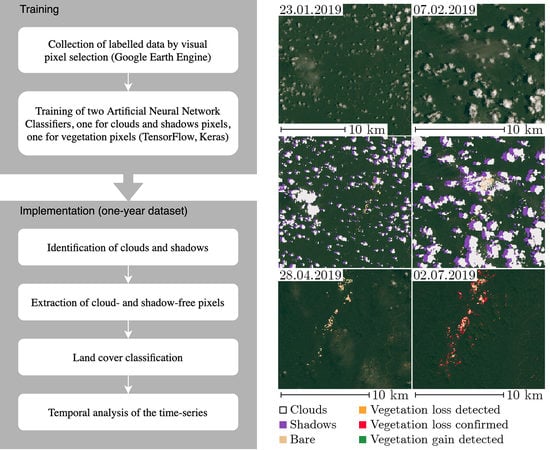
The objective of this paper was to propose a vegetation loss and gain monitoring strategy using cloud computing on Sentinel-2 data in a lowland tropical region strongly affected by the presence of high cloud percentage covers. It was hypothesized that the challenges posed by cloud and cloud shadow detection in the Amazon may be more effectively overcome with a region-specific model instead of an algorithm aiming to perform well globally. Therefore, the proposed strategy consists in (i) the identification and removal of cloud and cloud shadow pixels in order to increase the temporal density of analyzable images by using an artificial neural network classifier tailored to the region of interest, (ii) the identification of the green vegetation and bare soil/dry vegetation areas in the remaining clear pixels, and (iii) the implementation of an instrument to track vegetation loss and gain throughout the year while self-correcting for classification errors. This strategy is proposed as an initial step towards the development of an ecoregion-specific monitoring system that takes advantage of the possibilities offered by the development and spreading of cloud-computing technology and large remote sensing datasets.

2. Methods and Implementation

2.1. Study Site

The Sete de Setembro Indigenous Land (Figure 1), 250 km² of protected land at the border between Mato Grosso and Rondônia, is inhabited by the Suruí indigenous people of Brazil. It is surrounded almost integrally by cattle pastures and croplands and is especially vulnerable to illegal deforestation and forest degradation, as is generally observed for forest-covered land surrounded by cleared areas [10]. The Suruí people were among the first in the region to seek and implement a Reducing Emissions from Deforestation and Degradation program [10,34] and a large tree plantation program in formerly degraded areas. Nevertheless, illegal deforestation is still experienced on its territory [10]. The protection effort is complicated by the geographic extent of the area and by the inherent challenge posed by the detection of small-scale deforestation (e.g., artisanal-scale gold mining in river placers deposits, selective logging for timber production, and illegal extension of cattle pasture surfaces). In order to achieve better control over illegal intrusion, the Suruí villages are strategically located at the edges of the SSIL territory. Many villages are surrounded by legal plantations (e.g., coffee, cocoa, bananas) and cattle pastures exploited by the Suruí people. With the exception of these areas, the SSIL is covered by dense forest and crossed by the Rio Branco and several of its tributaries. The topography is mostly flat, with the exception of an 11-km-long vegetation-free protruding rock formation that appears distinctly on satellite images. The region is characterized by a tropical climate, with about 2000 mm of annual rainfall. A short dry season with less than 40 mm of monthly rainfall occurs from June to August and coincides with the occurrence of clear cloud-free satellite images.

2.2. Data

Optical remote sensing imagery from the Copernicus Sentinel-2 mission [35,36] was used in this study. The Sentinel-2 mission has a short revisit time of five days at the equator owing to its twin polar-orbiting satellites phased at 180° to each other. The Multi-Spectral Instrument (MSI) equipping the Sentinel-2 satellites passively collects 12-bit data on the sunlight reflection from the Earth within 13 spectral bands in the visible, near infrared (NIR), and short-wave infrared (SWIR) electromagnetic spectra with a high spatial resolution of 10 to 60 m, depending on the band [35,37]. The Sentinel-2 data product is available to users in two levels of processing: Level-1C (Top-Of-Atmosphere, TOA) and Level-2A (Bottom-Of-Atmosphere, BOA) in 100 km × 100 km granules. The Level-1C was chosen due to its systematic availability in the Google Earth Engine catalogue.

The SSIL is covered by four Sentinel-2 granules (T20LPN, T20LPP, T20LQN, and T20LQP) that overlap on a central point located at 10°53′24.0″ S, 61°07′48.0″ W. The study site (Figure 1) was constrained to a polygon defined by the following coordinates: 10°44′47.0″ S, 61°26′30.1″ W; 10°43′11.3″ S, 60°54′35.3″ W; 11°15′18.4″ S, 60°53′50.3″ W; 11°15′30.2″ S, 61°26′17.9″ W.

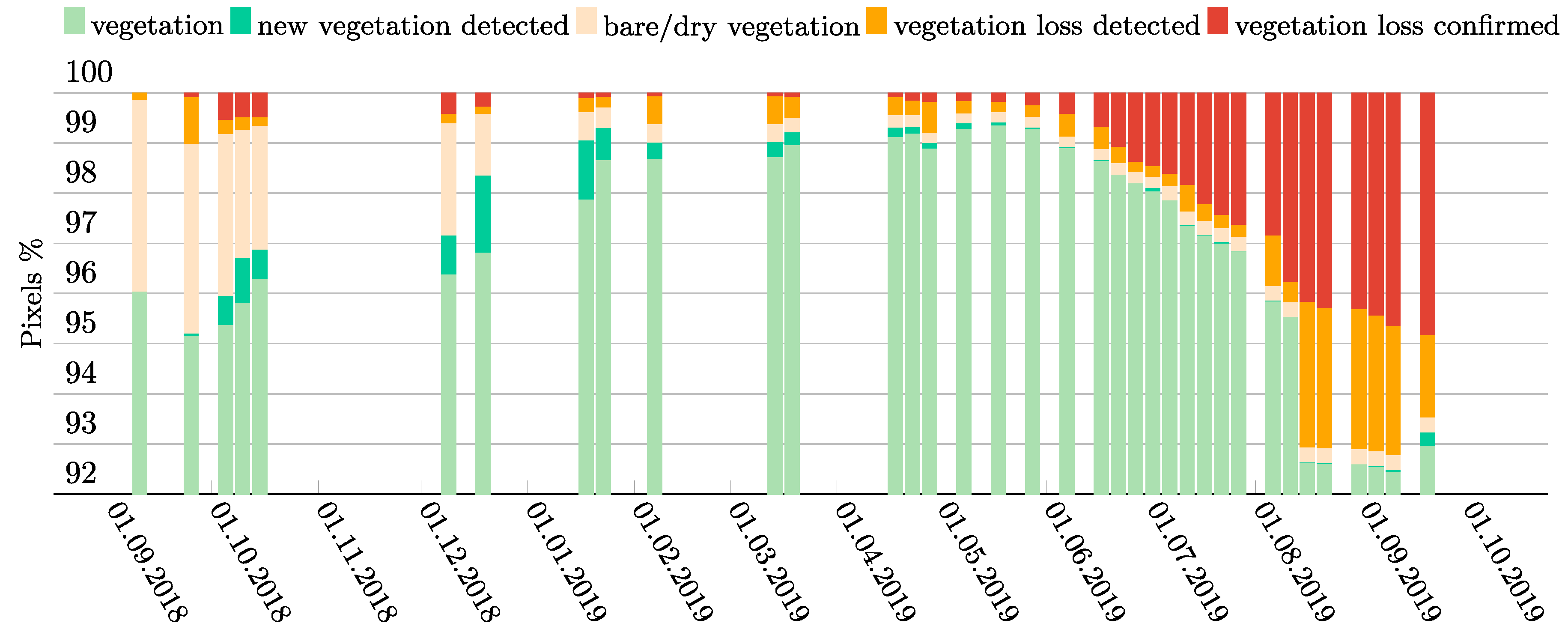
One year of data (05.09.2018 to 20.09.2019) was processed. During this time interval, out of 72 available scenes, 37 have a mean cloud cover of 50% or less and only 10 are completely cloud free (Figure 2). Such a yearly cloud cover percentage is representative for lowland tropical regions [19].

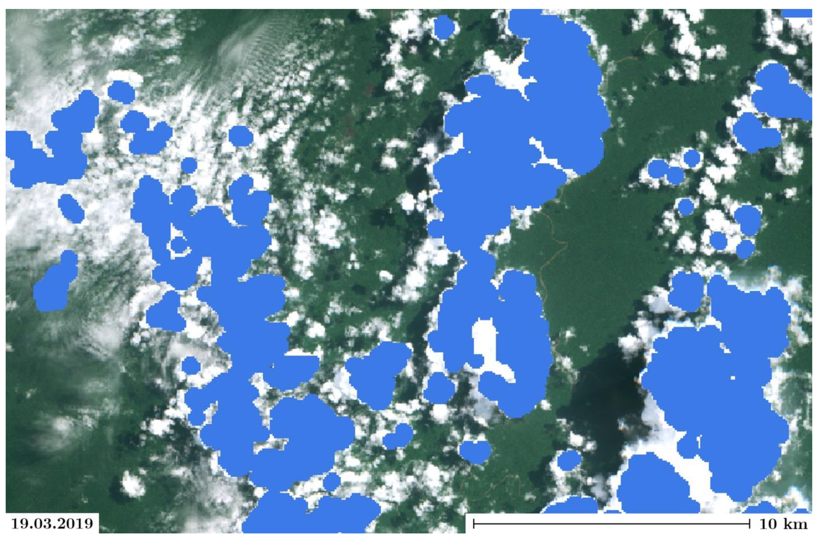
The Sentinel-2 data products are accompanied by a cloud-cover mask layer (band QA60, bitmask, Bit 10: opaque clouds, Bit 11: cirrus clouds) complemented by a mean cloud cover percentage given in the metadata of the granule [38]. However, as can be seen in Figure 3, the cloud mask fails to reliably identify the extent of the clouds and neglects their shadows entirely [21,22,39].

In addition to the Sentinel-2 bands, four spectral indices were computed for all images. The normalized difference vegetation index (NDVI):

NDVI = (NIR − RED)/(NIR + RED),

(1)

is used extensively to assess the general vegetation health and to distinguish vegetation types [40]. The normalized difference water index (NDWI):

NDWI = (GREEN − NIR)/(GREEN + NIR),

(2)

which was originally proposed for the delineation of open water features [41], was used to help distinguish water and cloud shadow areas. The enhanced vegetation index (EVI):

EVI = 2.5 ∙ ((NIR − RED)/((NIR + 6 ∙ RED − 7.5 ∙ BLUE) + 1)),

(3)

shows improved sensitivity compared to the NDVI in areas with high biomass and dense canopies [42]. Additionally, a cloud index (CI):

CI = (NIR + 2 ∙ SWIR1)/(BLUE + GREEN + RED),

(4)

as proposed by Zhai et al. [43], was used to help identify cloudy pixels, as these tend to be confused with bare soil areas.

2.3. Methodology

The selection of an image from the Sentinel-2 collection, its pre-processing, and part of the computing was performed with the Google Earth Engine (GEE), a cloud computing platform [15]. GEE allows relatively easy user-friendly access to high-performance computing resources for the processing of large geospatial datasets. The analyses are performed with an Application Programming Interface (API) available in JavaScript and Python languages. Freely available analysis-ready remote sensing data produced daily by the United States Geological Survey (USGS), the National Aeronautics and Space Administration (NASA), ESA, and other large public-funded agencies and data providers are included in the GEE catalogue. User-generated or uploaded data can be stored in Assets, a private data catalogue bound to the user’s account. The import and export of data can be performed through Google Drive (GD) or Google Cloud Storage (GCS) in a variety of formats. GEE-specific data types include Images (objects representing raster data, e.g., one scene from the Sentinel-2 dataset, composed of one or several bands), Image collections (stacks of individual images, e.g., a time series), Geometries (geographically defined vector data, such as points or polygons), Features (a geometry, e.g., points or polygons, and the associated properties), or Feature collections (stacks of features).

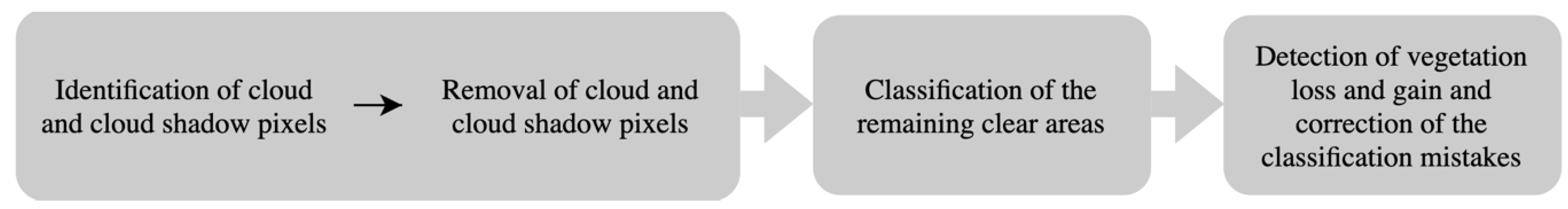
An automated classification strategy consisting in a two-step detection with a machine learning algorithm was developed and tested on a one-year set of Sentinel-2 images (Figure 4). The first step consisted in the identification of clouds and cloud shadows in order to isolate clear (i.e., cloud- and cloud shadow-free) pixels. This permitted the use of images with high cloud cover percentages, and, therefore, the extraction of maximum information from the time series. The second step consisted in a separate identification of two landcover categories (vegetation, bare soil/dry vegetation). To this end, two Artificial Neural Network (ANN) classifiers were trained in Google Colab notebooks using TensorFlow, a machine learning library developed by Google Brain with a focus on training and inference on deep artificial neural networks [44], and Keras, an open-source Python library aiming to facilitate the model construction and training process. The choice of the ANN approach was motivated by its reported high performance in remote sensing image classification, e.g., [27,45]. A detailed assessment of the use of ANNs in remote sensing was proposed by Mas and Flores [28]. After the initial classification, a false positive correction and vegetation evolution analysis were achieved with an automated comparison of the classified time series.

2.4. Training of the Classifiers

The GEE offers a Classifier package that handles supervised classification by several machine learning algorithms. Because it does not support large datasets or time series, it was not sufficient for the objectives of this study; however, it could be used to interactively identify the main classification challenges. After an initial assessment, it was determined that high reflectance surfaces, such as dirt roads, dry vegetation, and bare soil, were the landcover type most misclassified as clouds. Increasing the number of categories and labelled training points for these landcover types improved the identification of the cloud pixels; however, it also increased the classification errors between all other landcover types (roads, dry vegetation, green vegetation, bare soil). Because it was not possible to find a set of classification categories that allowed reliable identification of both the clouds and the vegetation, it was decided to train two classifiers.

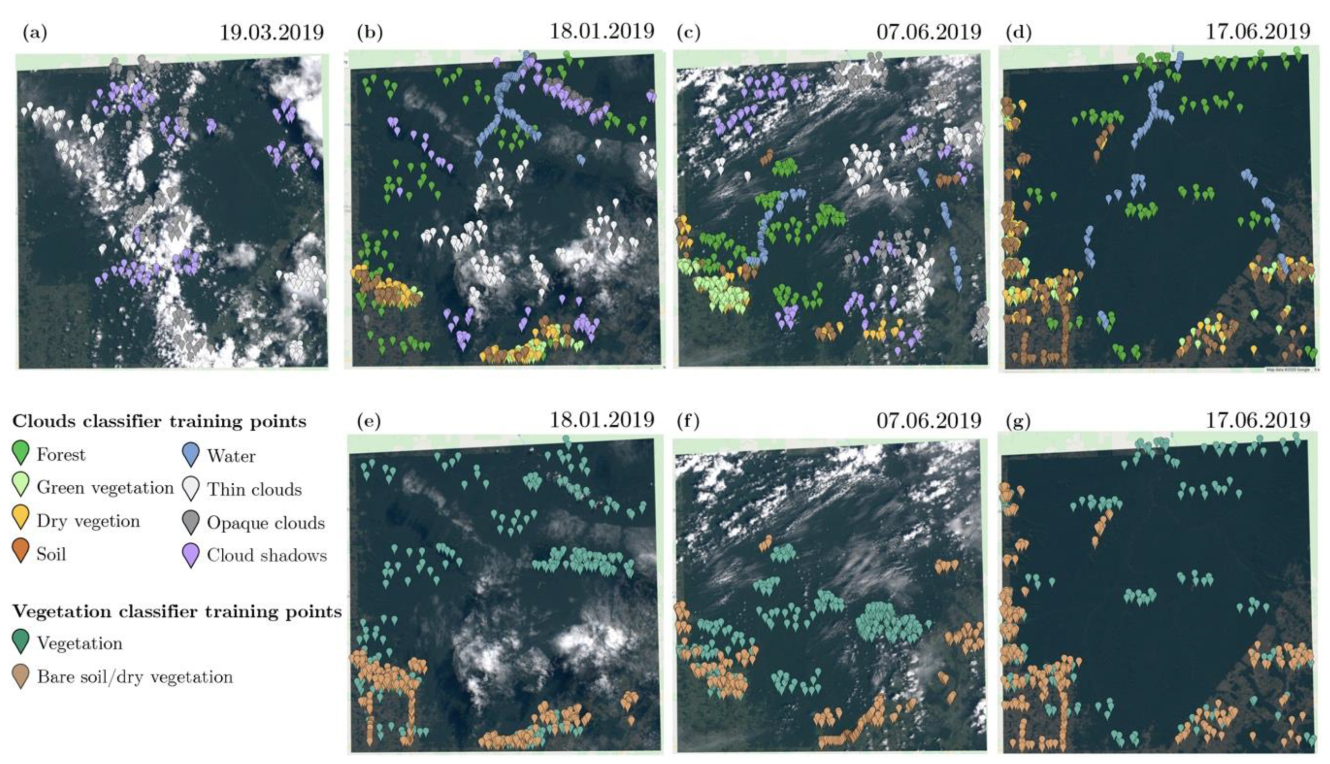
The aim of the first classifier was to reliably identify clouds and cloud shadows. A multi-class approach showed better results; therefore, seven classification categories (Forest, Green vegetation, Dry vegetation, Soil, Water, Shadows, Thin clouds, Opaque clouds) were chosen empirically with a trial-and-error approach in order to maximize the quality of the cloud and cloud shadow detection without special consideration for the quality or relevance of the classification for all other categories. Green vegetation refers to low vegetation, such as croplands or pastures; Dry vegetation refers to any vegetation that appears in brown tones in true color images and has low NDVI values; and Soil refers to bare soil and dirt roads. By contrast, the aim of the second classifier was solely to distinguish between bare soil/dry vegetation and any green vegetation. A binary output was chosen because the main interest was to distinguish healthy vegetation from all other landcover types, and a more precise identification of the vegetation categories and state was beyond the scope and time constraints of this project. The use of two classifiers allowed the challenge of reliably identifying a wide range of categories by using separate identification steps to be bypassed. Additionally, having two separate classifiers means that it is possible to use the vegetation classifier alone on clear scenes, which further limits the possibility of cloud and cloud shadow misclassification.

The training data for both classifiers were collected on the GEE by random visual pixel selection (Figure 5). No adjacent pixels were used and the distance between labelled points was at least 6 pixels. The four granules of the site were converted to a single image with the mean function, and all band values were converted to a range between 0 and 1. The previously described indices (i.e., NDVI, NDWI, EVI, CI) were added as bands. For the cloud and cloud shadow classifier, 2523 points were collected on four different scenes: Three cloudy scenes (18 January 2019, 19 March 2019, 7 June 2019) and one cloud-free scene (17 June 2019) (Figure 5a–d). The cloudy images were selected to be representative for both thin (i.e., cirrus) and opaque clouds. For the vegetation classifier, 1981 labelled points were collected on two cloudy scenes (18 January 2019, 7 June 2019) and a cloud-free scene (17 June 2019) (Figure 5e–g). The vegetation classifier has a binary output consisting of two classes: Vegetation and bare soil/dry vegetation. All labelled points’ feature collections were merged and sampled on their respective image. The two final collections thus obtained were randomized and attributed to training datasets (75%) or validation datasets (25%), and then exported to Google Drive in TFRecord format (an encoding format for binary records read by TensorFlow). The complete code can be found on Zenodo (https://0-doi-org.brum.beds.ac.uk/10.5281/zenodo.3766743).

In ANN algorithms, “neurons” refer to interconnected computational elements organized in successive layers, while activation functions refer to mathematical equations determining the output of a given layer of neurons. Both trained models were Keras sequential neural networks with two dense layers (consisting of 55 neurons and a rectified linear units (ReLU) activation function) and two dropout layers (rate of 0.2) to prevent overfitting, that is, excessive fitting of the model on the training data. The clouds model has a 16-neuron input layer and a 7-class output layer. The vegetation model has a 7-neuron input layer and a 2-class output layer.

2.5. Validation and Accuracy Assessment

The models were trained and validated on separate data. In total, 25% of the labelled data points, unseen by the models during training, were used to assess its performance during a validation step. The performance of the models on the previously unseen validation data was observed with a confusion matrix (see Section 3.1), where the predictions are compared with the actual labels.

As an additional step, a visual assessment of the classification was done by superposing each classification category on a true color (B423) image and checking the consistency of the results.

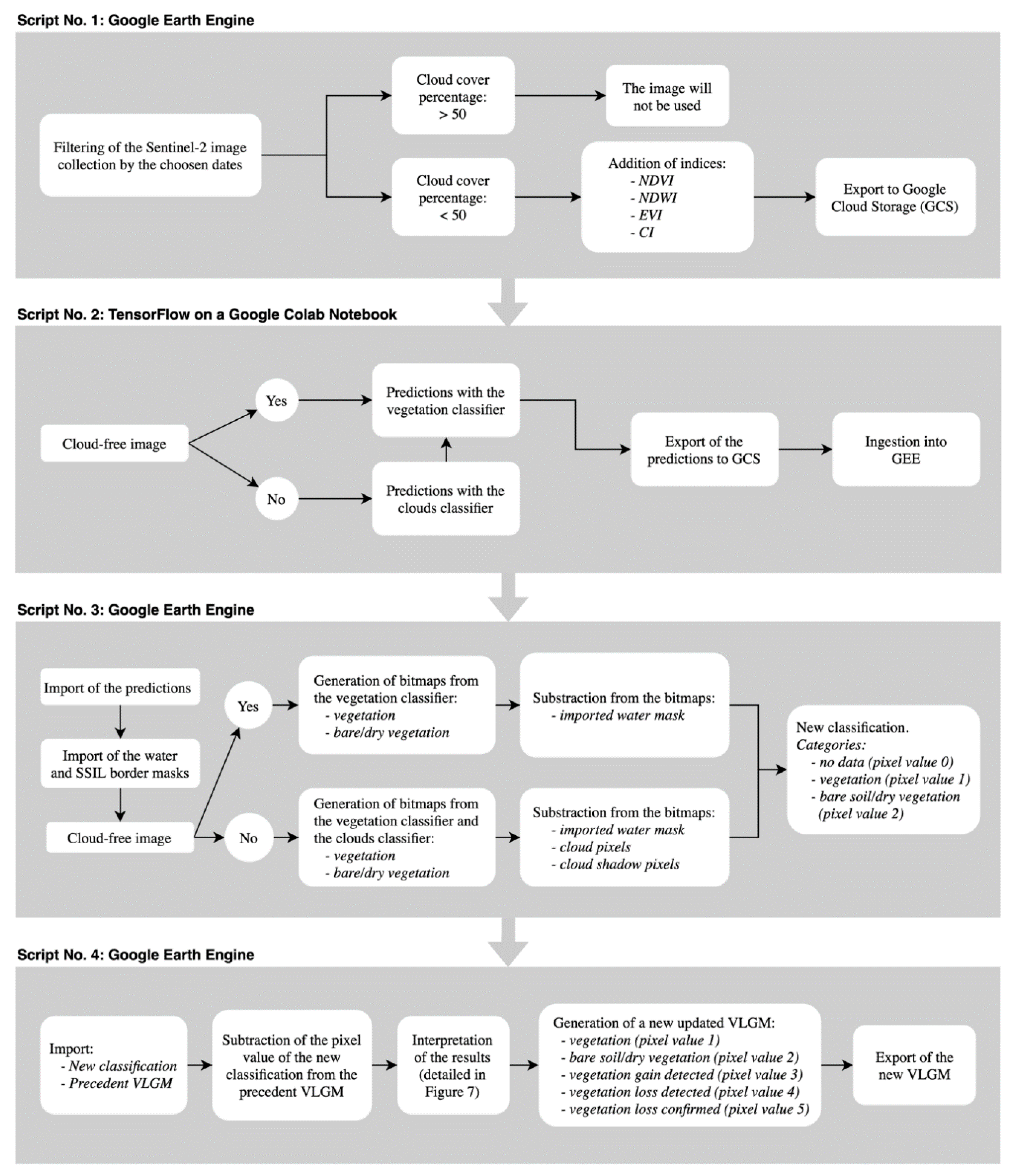
2.6. Data Processing

A workflow using the trained classifiers and consisting of four scripts (Figure 6), three running on GEE (JavaScript) and one running on a Google Colab notebook using TensorFlow and Keras libraries (Python), was implemented and applied to one year of data (5 September 2018–20 September 2019).

The first script (JavaScript, GEE) allowed the selection and export of a Sentinel-2 image to GCS with all bands and indices. An arbitrary threshold value of 50% cloud cover, based on the mean cloud cover estimate from the Sentinel-2 metadata, was set. Above this threshold value, the image was considered too cloudy for analysis and was not automatically exported.

The second script (Python, Google Colab notebook) ran the trained classifiers on the image. The image was retrieved from GCS, parsed, pre-processed, classified, written to a TFRecord file on Google Cloud Storage, and ingested into the GEE Assets. For clear images, the cloud and cloud shadow classifier was not used.

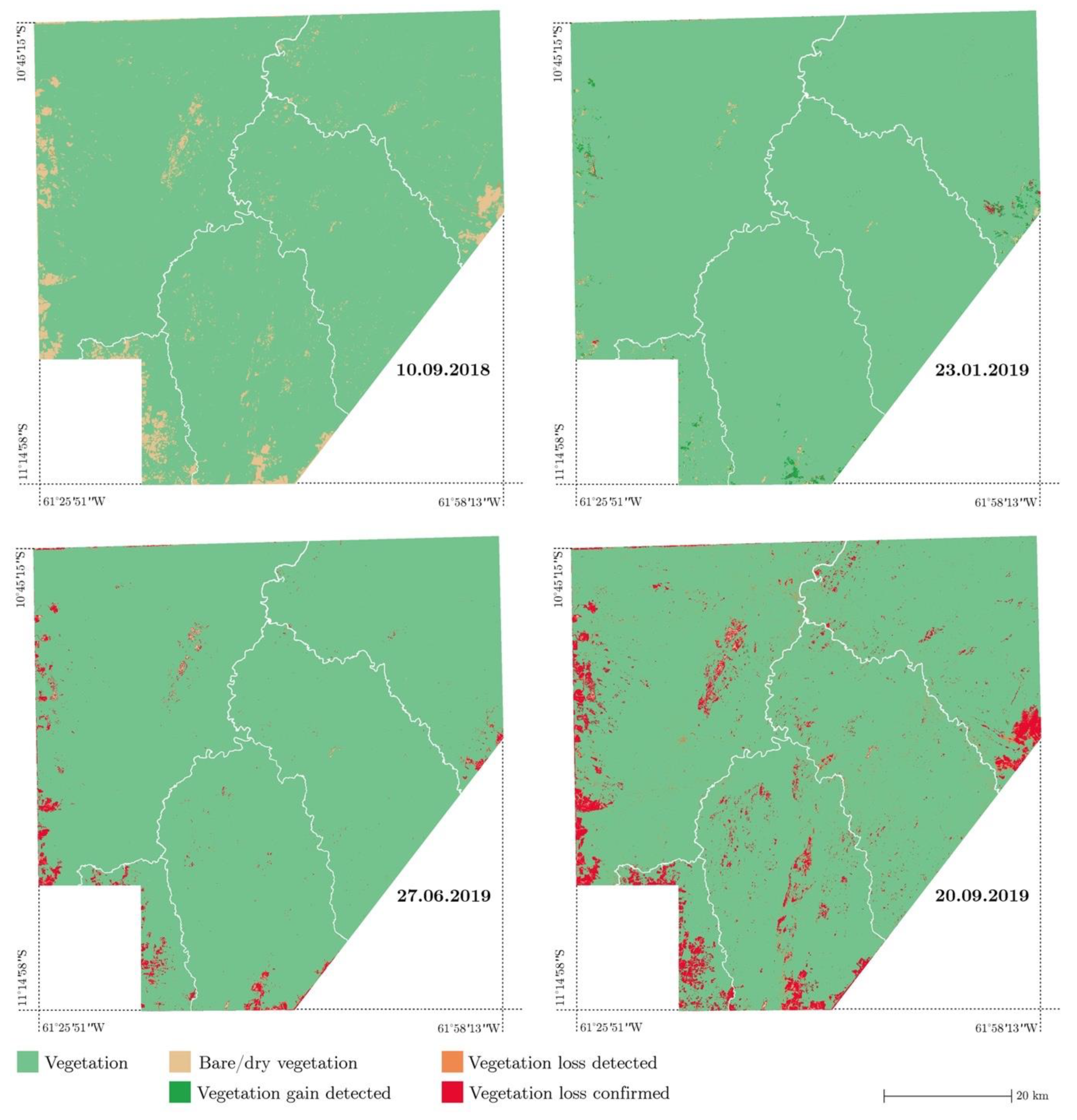
The third script (JavaScript, GEE) processes the prediction outputs and produces a unified synthesis of the vegetation and cloud classification, completed by a raster water mask hand drawn using the GEE interactive geometry tools and stored in the Assets. From the cloud classifier output, only the values of the pixels classified as opaque clouds, thin clouds, shadow, and water were used; all other classes were discarded. The opaque and thin clouds were combined into a single "clouds" class. The shadows and water pixels tended to be confused by the detection algorithm, that is, shadows were sometimes classified as water and vice versa. Because this misclassification did not extend to other categories, both classes were combined in a unique "shadow" class. This pragmatic decision could be taken because the actual water cover on the site is both scarce and stable over time and could therefore easily be drawn by hand. Two images were prepared for export: A first classified image for visualization and archiving purposes, including the categories Clouds, Shadows, Bare soil/dry vegetation, Vegetation, and Water; and a second classified image destined for further analysis, from which clouds, shadows, and water pixels were removed and replaced by a No data category.

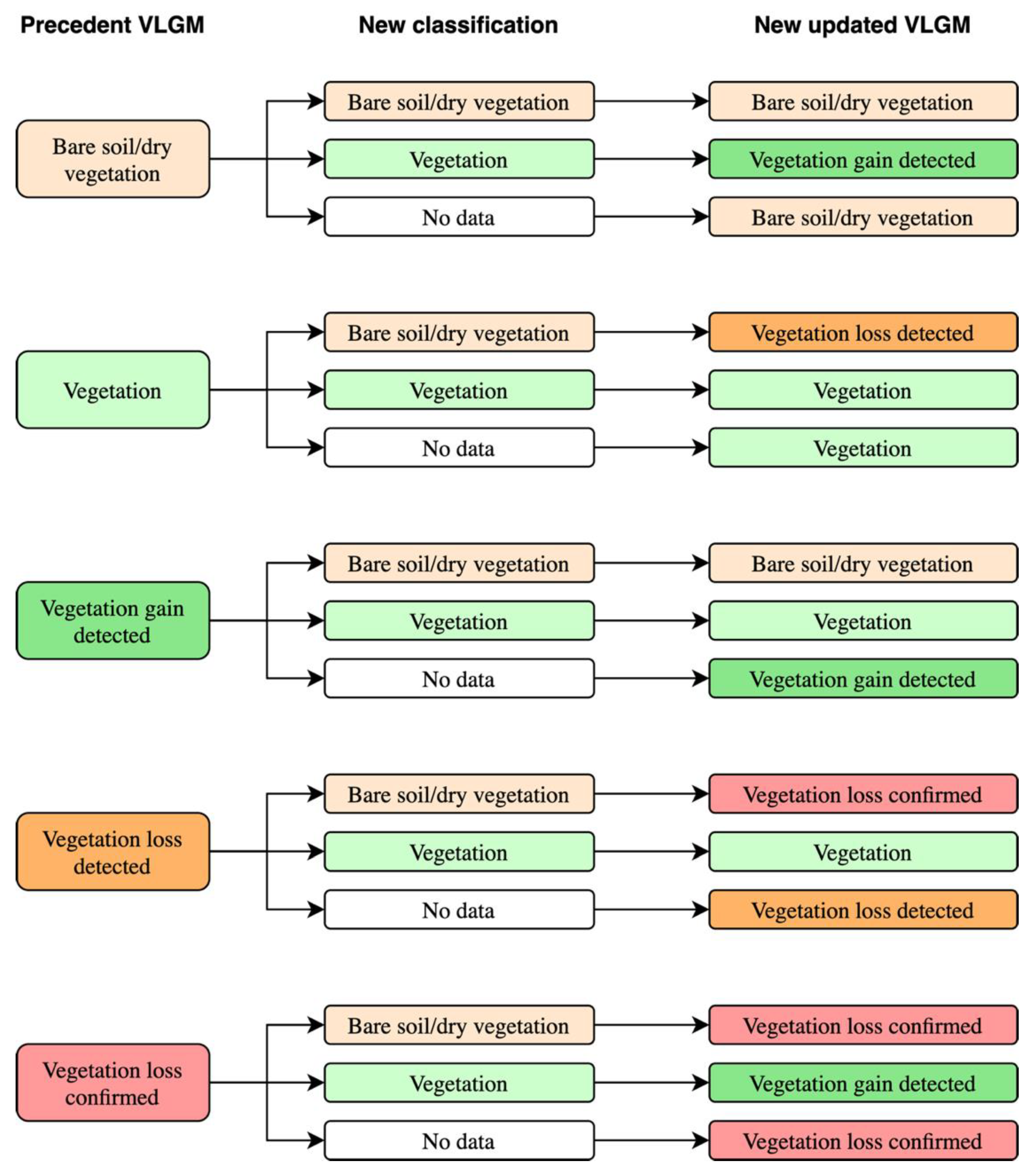
The fourth and final script (JavaScript, GEE) used the classified image in order to create a dynamically updated vegetation loss and gain map (VLGM) comprising the categories Bare soil/dry vegetation, Vegetation, Vegetation loss detected, Vegetation loss confirmed, and New vegetation detected and corrected for detection errors. In order to be confirmed, a loss or gain had to be detected twice in a row (Figure 7). If no data were available in the subsequent image classification, for example, because the area was covered by clouds, the detected status was maintained instead of being confirmed or discarded.

The complete code can be accessed directly in the Google Earth Engine code editor (https://colab.research.google.com/drive/1HgCUiKDqeNI-P1TG4iOK69R75HrkCw1r) or on Zenodo (https://0-doi-org.brum.beds.ac.uk/10.5281/zenodo.3766743).

3. Results

3.1. Models

The confusion matrices produced with the models’ predictions showed that 60% to 85% of the pixels were correctly classified (Figure 8). The clouds and the cirrus were almost only misclassified as each other and as shadows, which is acceptable for the desired use of the model as the categories were later merged into a single mask. Once merged into a single category, the misclassified clouds and cloud shadow pixels dropped to <5%. Pixels corresponding to forest landcover were classified as shadows 25% of the time, presumably when they were darker due to self-shading or the topography. The vegetation and bare soil/dry vegetation classifier correctly classified 86.7% of the forest pixels and 79.5% of the bare soil/dry vegetation pixels. Soil/dry vegetation was misclassified as forest 20.5% of the time. The overall accuracy for both models is >0.95 for the training and validation data.

The visual assessment of the performance of the cloud and cloud shadow classifier also showed very promising initial results on the SSIL dataset. Both opaque and thin clouds were reliably detected and, after visual assessment, showed much better performance than the Sen2Core cloud mask included with the data (Figure 9 and Figure 10). Our cloud classifier detected cloud cover of more than 1% in 23 of the 37 analyzed images (Figure 9). In 13 cases, our classifier detected substantially more cloud cover (between 5 and 25 percentage points) than the Sen2Cor algorithm. In six cases, cloud cover was detected by our classifier but not by Sen2Cor, both in the presence of fire smoke and in the presence of cirrus clouds. In three cases, the detected cloud cover percentages agreed well. In one image (15 October 2018), Sen2Cor detected a large cirrus cover that our classifier did not detect. As can be observed in Figure 10, these differences can be primarily attributed to the underdetection of cloud pixels by the Sen2Cor algorithm. Because, in contrast to Sen2Cor, our classifier also identifies cloud shadows, this means that the area that can be masked before further analysis is substantially larger when our classifier is used (Figure 9).

Due to the choice of training data, the detection was very sensitive, with a tendency to classify pixels as clouds even when the cover was very thin. This choice allowed for a lower occurrence of vegetation misclassification due to altered radiometric signals. The shadow area underneath the clouds was very precisely detected as well. Some shadows due to the topography were additionally detected when the cloud and cloud shadow classifier was run. Figure 10 also shows the output of the cloud and shadow classifier in periods of forest fires (10 September 2019). The smoke cover, which is not identified by the Sentinel-2 cloud cover algorithm, was poorly classified as shadows or clouds. This classification occurred both when the cover was thick and thinner. Therefore, in the present state of our model, such imagery is not suited for vegetation detection. Because our proposed system includes a dynamic vegetation observation step (see next sections), the cloud and cloud shadow classification errors could be corrected at later stages.

3.2. Increase of the Temporal Data Density

The use of a cloud and cloud shadow classifier allowed the inclusion of images with a cloud cover percentage up to 50%, which considerably increased the temporal resolution from 10 (clear images exclusively) to 37 images (50% cloud cover or less) over one year. The percentages of pixels that could be used for analysis over the whole dataset are shown in Figure 11.

The 50% threshold value for the cloud cover percentage showed satisfactory results, that is, a low occurrence of false positives in the vegetation detection. When the cloud concentration over a given area was especially high, false positives did occur. These, however, could be corrected in the comparison process (Figure 12).

3.3. Detection of the Vegetation Loss and Gain

The bare soil and vegetation algorithm showed valid results as well, as it was able to detect individual pixels and was relatively sensitive to drier areas of the forest, with a tendency to detect rather more than less vegetation loss (Figure 10, lower row). In particular, areas covered with lower vegetation (e.g., croplands or cattle pastures), which are highly susceptible to seasonal changes, were detected by the model during the drier season, especially August and September. This sensitivity is justified by the fact that areas covered by trees show only limited drying and change throughout the year. Therefore, any dry or bare areas detected by the model are presumably bare of primary forest, even if they are covered by low vegetation, such as croplands, which makes it suitable for the observation of deforestation by illegal extension of cattle pastures.

The vegetation loss and gain detection system (Figure 12 and Figure 13) allows a dynamic interpretation of the time series and updates all categories, including the areas previously classified as Bare soil or Vegetation loss confirmed where new vegetation was detected, which limits the accumulation of outdated information over time. It also accounts for the evolution of the low vegetation areas (pastures, croplands) over the seasons. On the 23 January 2019 image, new vegetation starts to appear and is identified by the model (green area on the left-hand side of the image). On the 28 April 2019, the vegetation gain has been confirmed and removed from the map. Indeed, on the true color image in the top part, the vegetation is visibly healthy. On the 2 July 2019 image, senescence and drying-out of the vegetation started occurring again—vegetation loss, in red, has been confirmed. A new vegetation loss area, on the right-hand side, has been detected and partially confirmed as well. On the 11 August 2019 image, the vegetation loss has visibly progressed both on the right- and left-hand sides of the image.

The evolution of the vegetation on the SSIL throughout one year (September 2018–September 2019) can be seen in Figure 13 and Figure 14. At time zero of the monitoring, about 96% of the SSIL was covered by forest and green vegetation, while 4% was covered by other types of surfaces (bare soil, dry vegetation, settlements) (Figure 14). During the wet winter season, although regular observation of the landcover was hindered by the frequent occurrence of cloud covers superior to 50%, a trend is distinctly visible. The green vegetation cover expands, reaching more than 99% in May 2019. From June 2019 onwards, the percentage of dry and bare areas started increasing again until reaching values comparable to the previous year. During August 2019 and the first part of September 2019, a very high percentage of detected but unconfirmed bare/dry vegetation appeared due to the interference of forest fire smoke. On the last analyzed image, this category decreases again due to the availability of clearer images. In mid-September 2019, at the end of the monitored period, the area covered by confirmed bare soil/dry land increased by more than 0.5% compared to mid-September 2018. This excess loss of vegetation was confirmed and attributed to a localized deforestation event by a Suruì representative (February 2020, personal communication).

The vegetation loss and gain detection system is a proof of concept. Any shortcomings of the classification algorithms are therefore transferred to it and only the comparison of data over time can improve the quality of the final output. This, however, also means that any improvement done on the models will seamlessly transfer to the vegetation loss and gain system without the need for additional adaptation work.

4. Discussion

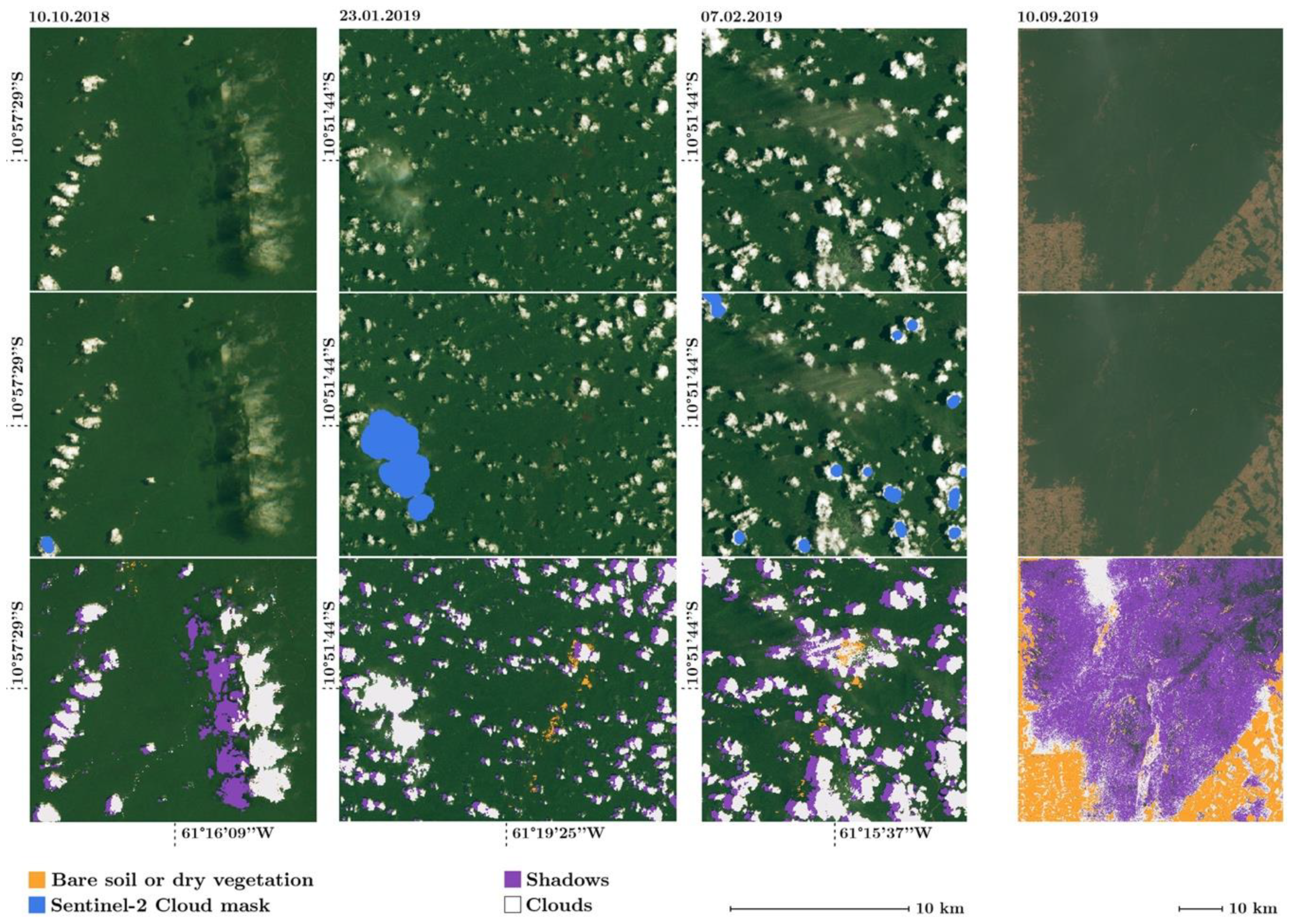
In its present state, the model is able to identify vegetation loss and gain while reliably filtering out cloud and cloud shadow pixels. The vegetation detection efficiently distinguishes forest from bare soil and senescence-prone biomass, such as cattle pastures, shrubs, or plantations. Moreover, it provides an efficient false positive detection system, which prevents the accumulation of detection errors over time. Owing to its coupled vegetation/cloud and shadow detection systems, useful information can be extracted not only from cloud-free scenes but also from images with a high cloud cover percentage, which, combined to the use of the short revisit time of the Sentinel-2 mission, allows for a high temporal resolution. This is especially valuable in lowland tropical regions, where optical satellite imagery is vulnerable to excessive cloud cover. The threshold value of 50% is indicative and could be selectively increased when areas of interest, such as known vulnerable zones, are clear, even when the rest of the scene is not. Because of the precision of the outline of detected clouds, areas in the holes of the clouds could be included as well (Figure 10). The comparison system provided a time series showing the evolution of the vegetation over time. Outdated information, e.g., previously bare areas reclaimed by vegetation growth, were removed from the map through the correction mechanism while newly bared or dried-out surfaces were signaled. This allowed the observation of a distinct trend in the vegetation loss and gain even during the cloudy winter months. In September 2019, a realistic increase in vegetation loss compared to September 2018 could be observed.

The use of GEE and Google Colab notebooks allows the process to be run integrally from a common web browser with an ordinary domestic internet connection without the necessity to download any data on the personal computer of the user. This makes the system suitable for use in remote locations, provided an internet connection can be established (the use of a laptop with the “mobile hotspot” function of a mobile phone connected to the internet has proven to be sufficient without inducing any significant treatment time increase).

Our workflow allowed us to successfully remove cloud and cloud shadow pixels from analyzed images, thus significantly increasing the data density. The remaining pixels could be realistically classified and used in an automated vegetation loss and gain monitoring with a self-correcting function that led to the identification of a vegetation loss due to actual deforestation. This model can therefore constitute a powerful monitoring tool to assist in the prevention and assessment of deforestation and forest degradation. As all three steps of the strategy are separated, a more precise classification of the vegetation categories, which was outside the scope of this project, could be further improved in the future development of an ecoregion-specific monitoring system.

Compared with other studies, where underdetection of clouds and cloud shadows by globally targeted clouds detectors was challenging in lowland tropical regions [18,21,22], our target classifier combined with a false positive/false negative detection strategy yielded satisfactory results over the region of study.

The first limitation of the system in its present state is its malfunction in the presence of forest fire smoke, which has proven especially relevant in the chosen one-year dataset, as the intensity of the 2019 fire season was high. The vulnerability of the model to the signal perturbations due to a high fire-induced aerosol concentration in the drier season (August–September) could be overcome with an additional classification category or with a dedicated classifier. The second limitation is the lack of distinction between anthropogenic and seasonal vegetation loss. Because the natural seasonal cycles of vegetation senescence and regrowth dominate several areas of the SSIL, notably in the legal cropland zone, in the vicinity of vegetation-free rock formations and along the rivers, the signal can be excessively cluttered by natural ecological processes, which hinders the detection of smaller scale anthropogenic forest degradation. Therefore, this limitation implies that a final interpretation effort is still required of the user. This distinction could be improved with two complementary strategies. The first would consist in the hand mapping of known legal low vegetation areas. The produced mask would allow the removal of these areas from the analysis entirely. In order to implement such a solution, collaboration with the inhabitants of the SSIL is of paramount importance, as the legitimacy of such masked areas cannot be deduced from satellite data alone. This strategy may imply that the model will function best in well-known areas, where collaboration with local inhabitants is possible, and its extension to other parts of the eco-region could be limited by a loss of classification quality. The second strategy would be to include different types of data into the classification system, such as radar data. As the Sentinel-2 mission, the Sentinel-1 mission consists of two twin satellites orbiting at 180° from each other. These satellites are equipped with a C-band synthetic-aperture radar (SAR) instrument that collects observational data regardless of the weather, as it is not susceptible to the cloud cover, with a revisit time of 12 days for each satellite [46,47]. SAR imaging can be used to produce 3-D elevation imagery after processing. Including such data in the classification model would allow filtering of the vegetation loss signal by isolating alerts that correspond not only to dry bare land but also to an elevation loss due to the felling of trees [48]. As an additional advantage, radar imagery can be used to very effectively identify water, which would further improve the quality and resolution of the detection and eliminate yet more false positives, and to improve the detection of cloud shadows, as in the current state of the model, shadows due to the topography are partially detected as well. Moreover, for the analysis of a larger dataset spanning several years, a variability index for individual pixels could be introduced as an additional tool for quality control and analysis improvement. In addition to visual pixel selection by hand, the collection of training data could benefit from the inclusion of a larger variety of data sources, such as on-site observational data or participative citizen science [49,50], and by collection and organization of the reference spectra in a spectral library [51]. This would allow for further finetuning of the model and an improved classification quality.

Owing to the rapid development of solutions that allow one to train a machine learning algorithm without extensive prior knowledge in programming or costly investments in fast computers, the training of a highly specialized classifier is now an implementable solution to support conservation efforts in a given area. This project represents a first step in the development and implementation of a specialized ecoregion-specific monitoring system. Further development and implementation of such a system could be performed either with the GEE or with a Data Cube on Demand (DCoD) approach, as proposed by Giuliani et al. [52]. The implementation in a DCoD system would allow heightened ownership and control over the processed data, as well as a higher level of flexibility because machine learning algorithms could be implemented directly into the structure.

5. Conclusions

Thanks to its high spatial, temporal, and spectral resolutions, Sentinel-2 is a potentially powerful tool for the monitoring of deforestation and forest degradation. Nevertheless, its application in lowland tropical regions is limited by the inherently frequent cloud cover, which greatly impacts the temporal resolution of the images. Even though a low revisit time increases the chances of obtaining clear images, the coverage outside the drier season (July–September) is insufficient to guarantee regular monitoring. Therefore, to fully take advantage of the Sentinel-2 products and obtain the highest density of data, cloud and shadow pixels must be reliably identified and removed from the analysis in order to extract the informative areas of the image. If such processing can be implemented, the obtained dense time series allows for effective and regular tracking of vegetation dynamics through time, including, for example, seasonal variations, deforestation, and forest regrowth.

The proposed coupled vegetation/cloud and cloud shadow classification model was able to identify vegetation loss and gain while reliably filtering out cloud and cloud shadow pixels. The vegetation detection system efficiently distinguished undisturbed forest from bare soil and senescence-prone vegetation for a test batch of one year of Sentinel-2 data for the SSIL territory. The false positive/false negative detection system prevented the accumulation of errors over time and offered an overview of the seasonal evolution of the vegetation on the SSIL. It is a promising first step towards a specialized ecoregion-specific vegetation dynamics and deforestation monitoring system supporting conservation efforts.