Multiplatform-SfM and TLS Data Fusion for Monitoring Agricultural Terraces in Complex Topographic and Landcover Conditions

 , , ,
, , ,  and
and 
Abstract
:
1. Introduction
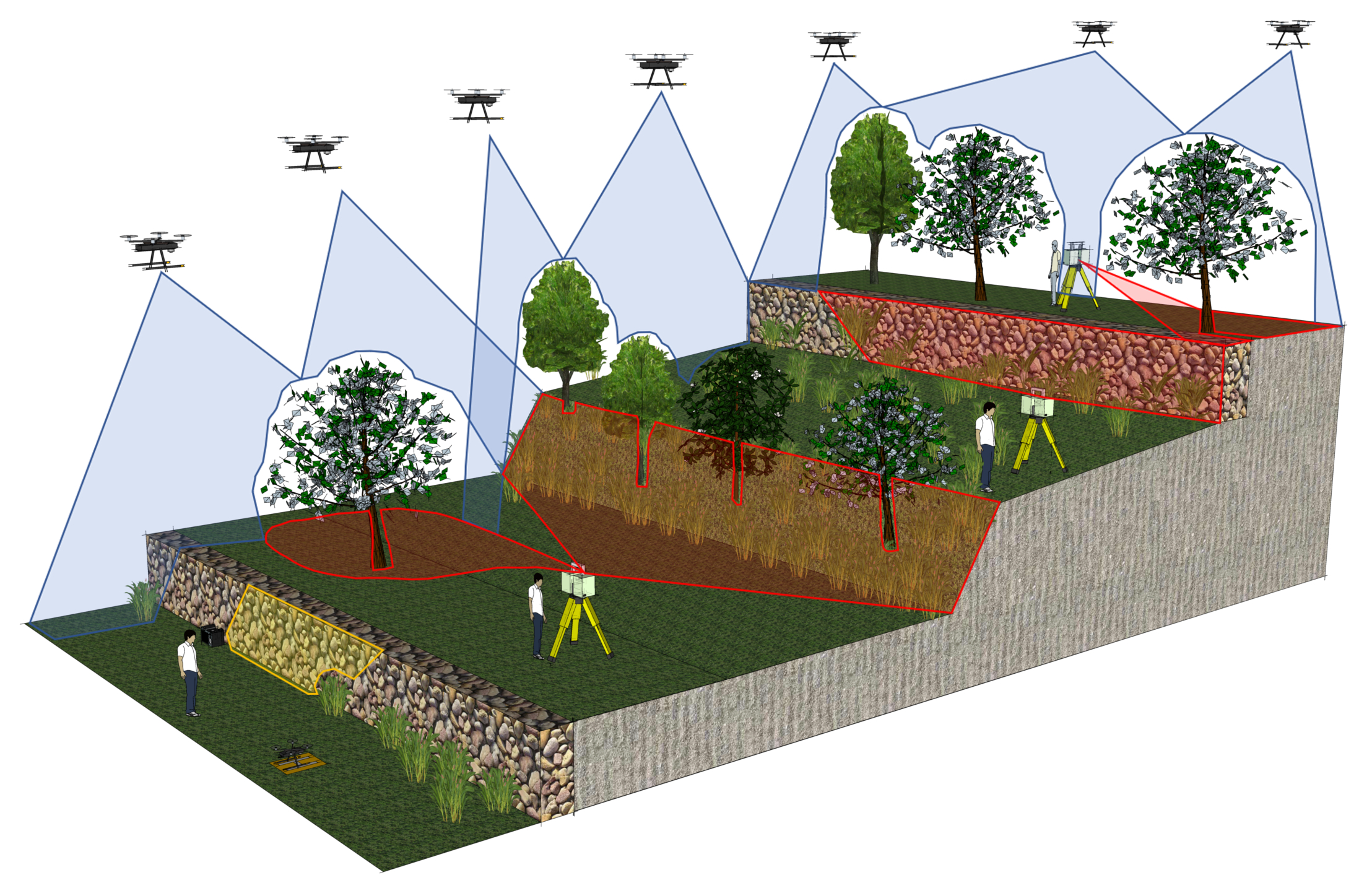
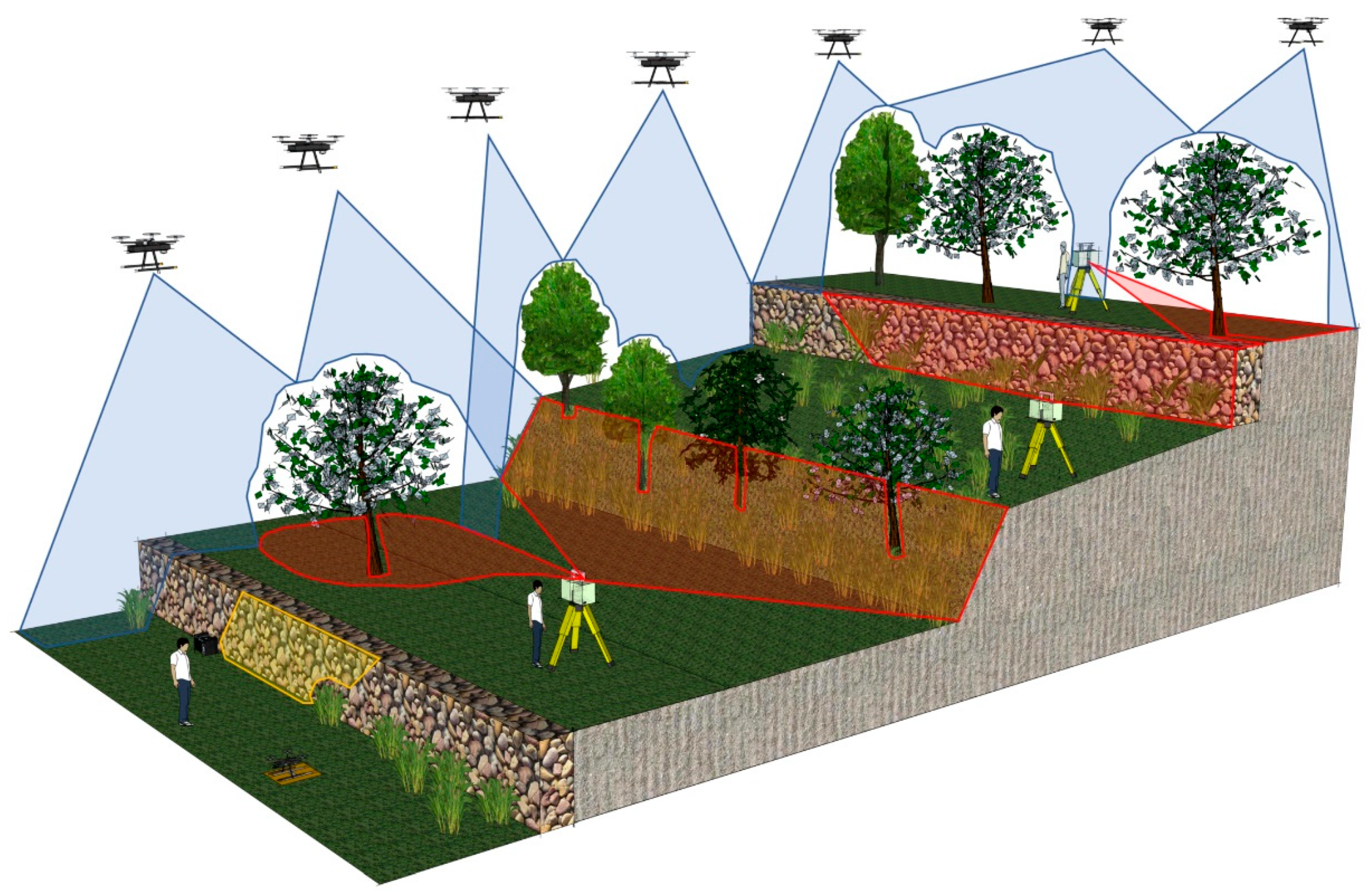
2. SfM–TLS Data Fusion
3. Data and Methods
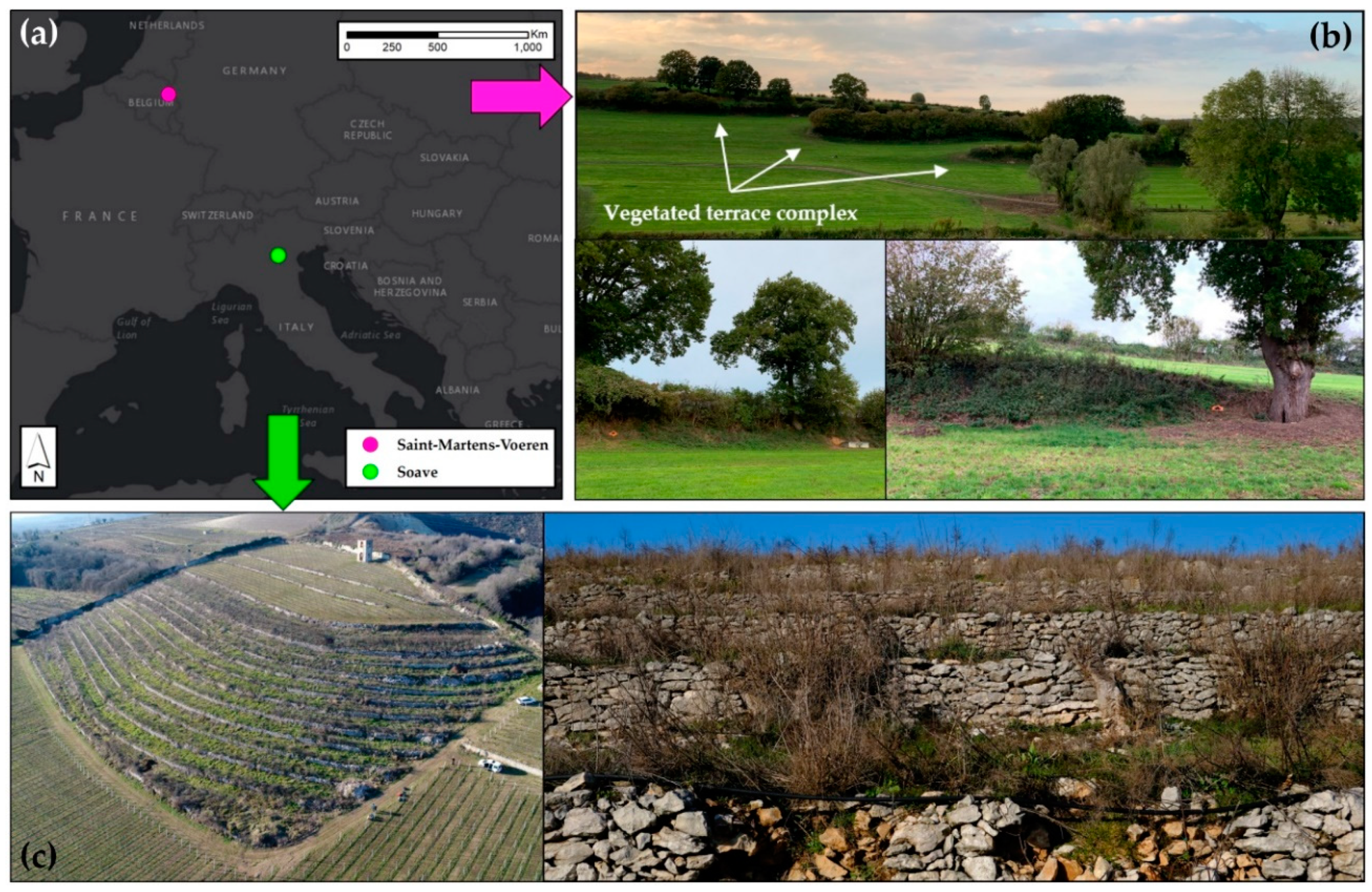
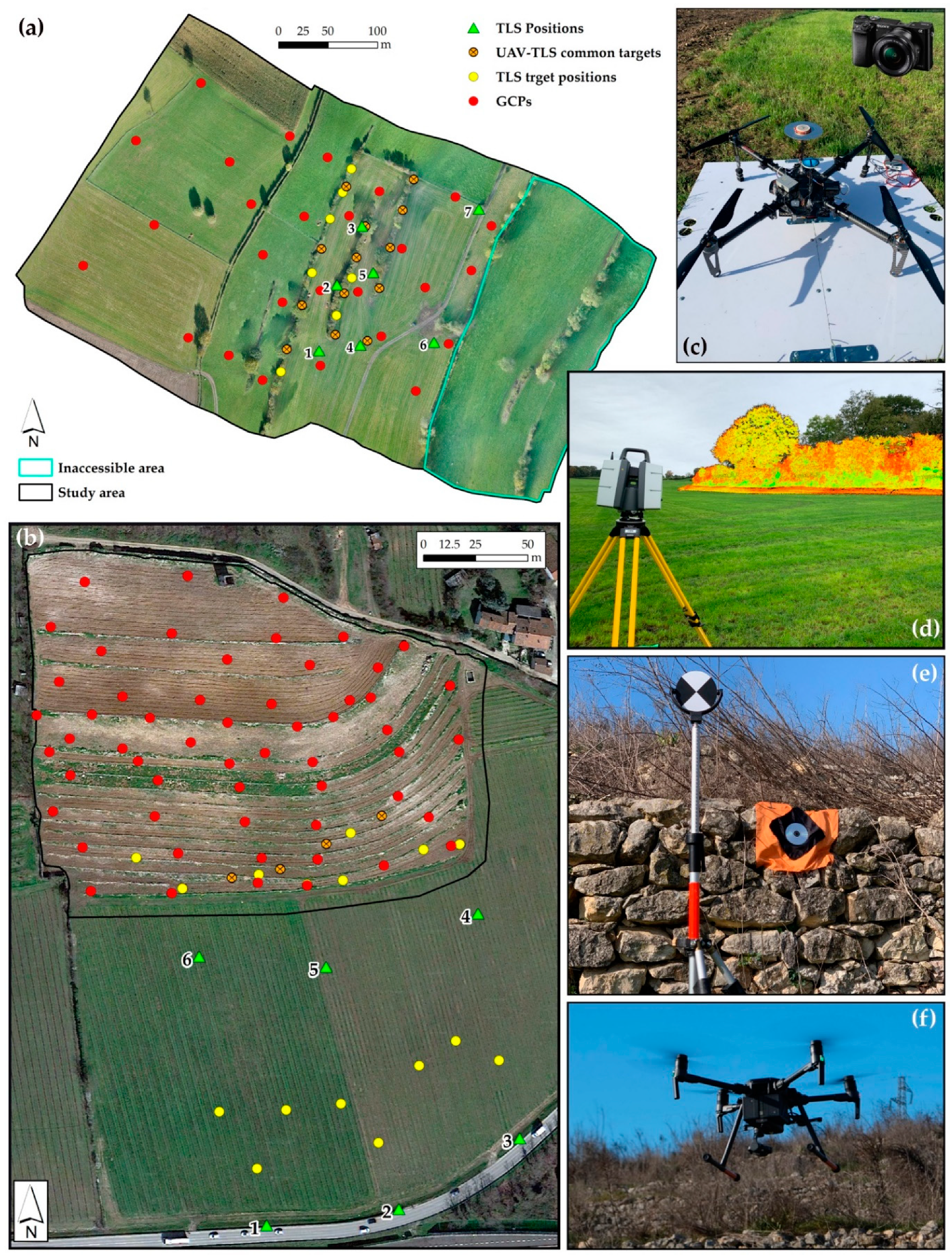
3.1. Study Areas
3.1.1. Belgian Study Area
3.1.2. Italian Study Area
3.2. Data Acquisition
3.2.1. SfM Surveys
3.2.2. TLS Surveys
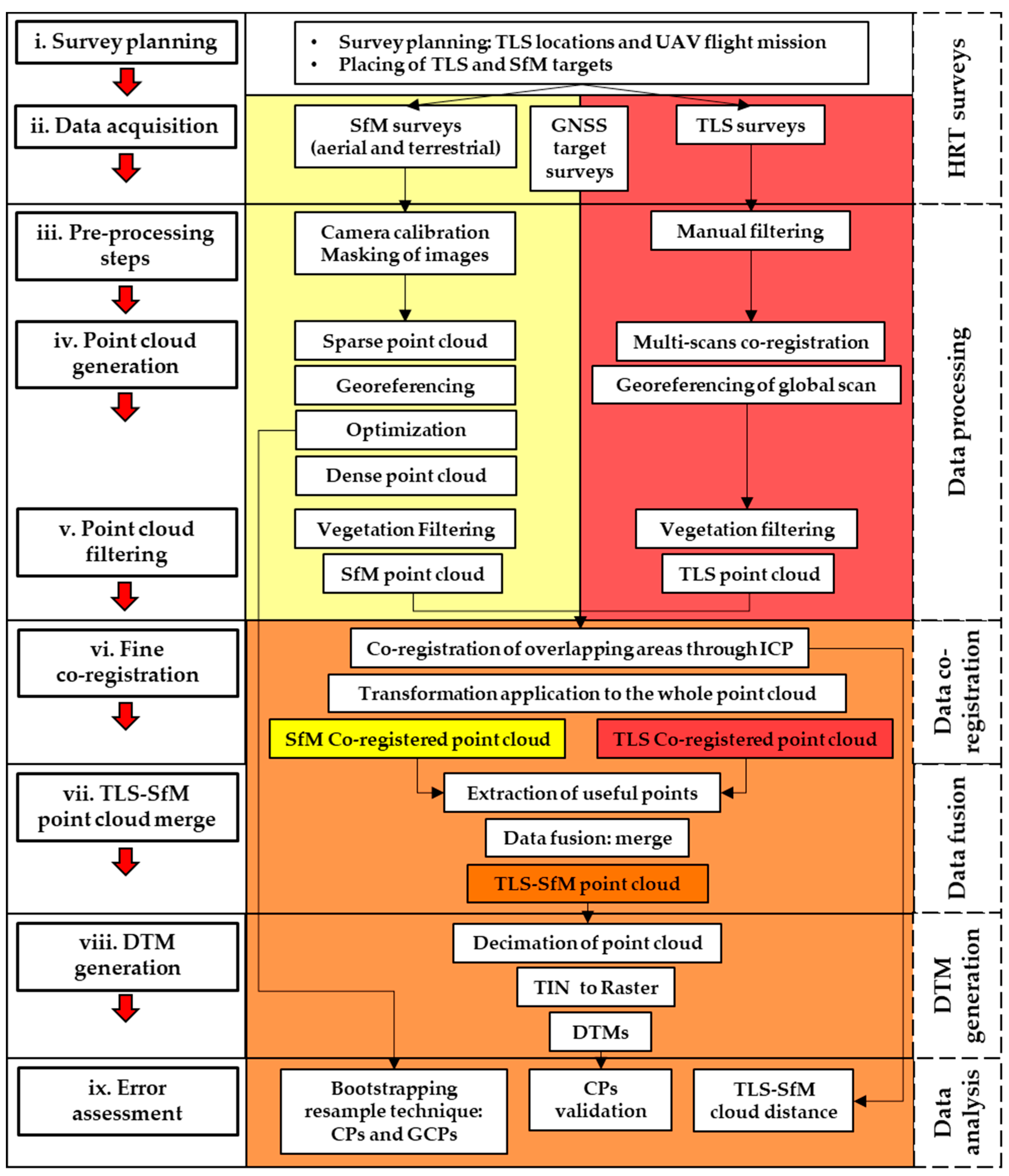
3.3. Data Processing
3.3.1. SfM Processing
- GCP solution: The traditional solution of the GCP coordinates (evaluating the level of GCP uncertainty before including these data to avoid adversely affecting data accuracy [58]) was employed to scale and georeference the SfM-derived point cloud. This result was obtained by using a seven-parameter linear similarity transformation, through locating and manually marking GCPs on at least two photographs. In this case, some of the GCPs (one-third) were used as control points (CPs) to provide an independent measure of accuracy.
- PPK solution: The camera positions from PPK data encoded in the images were used. Here, no information on GCPs was exploited.
3.3.2. TLS Processing
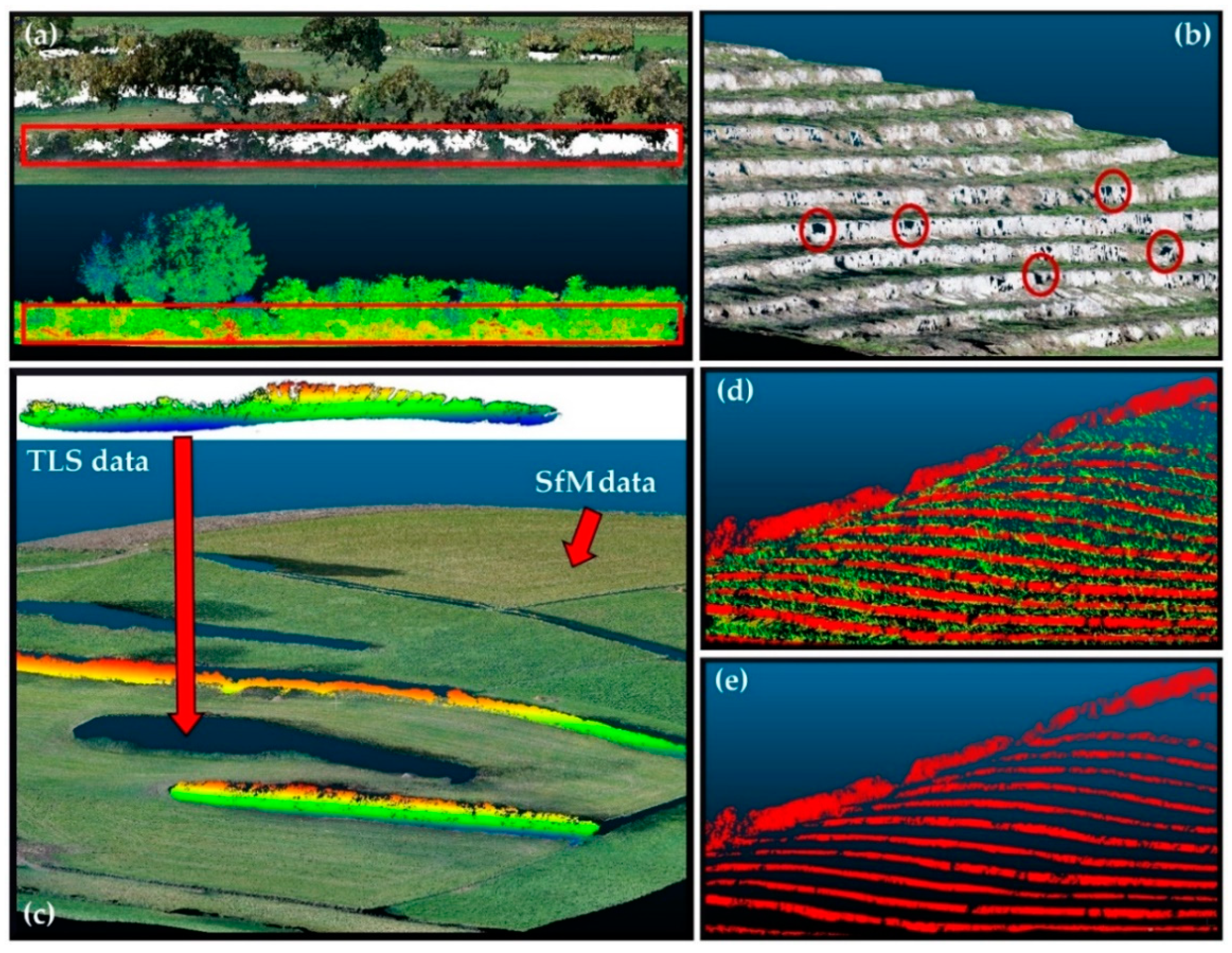
3.4. Coregistration and Data Fusion
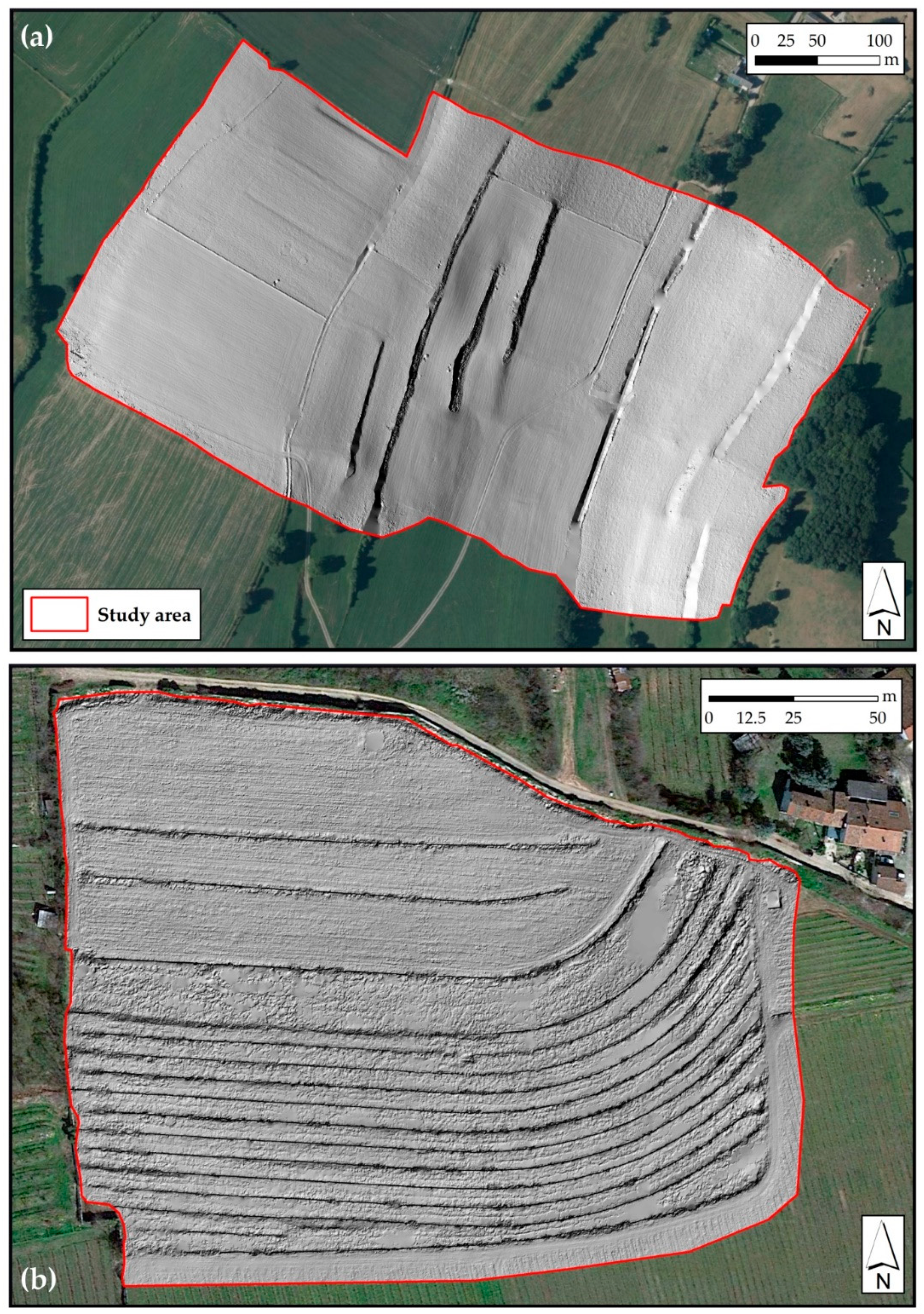
3.5. DTM Generation
3.6. Data Analysis
4. Results and Discussion
4.1. SfM Outputs
4.2. Coregistration Process
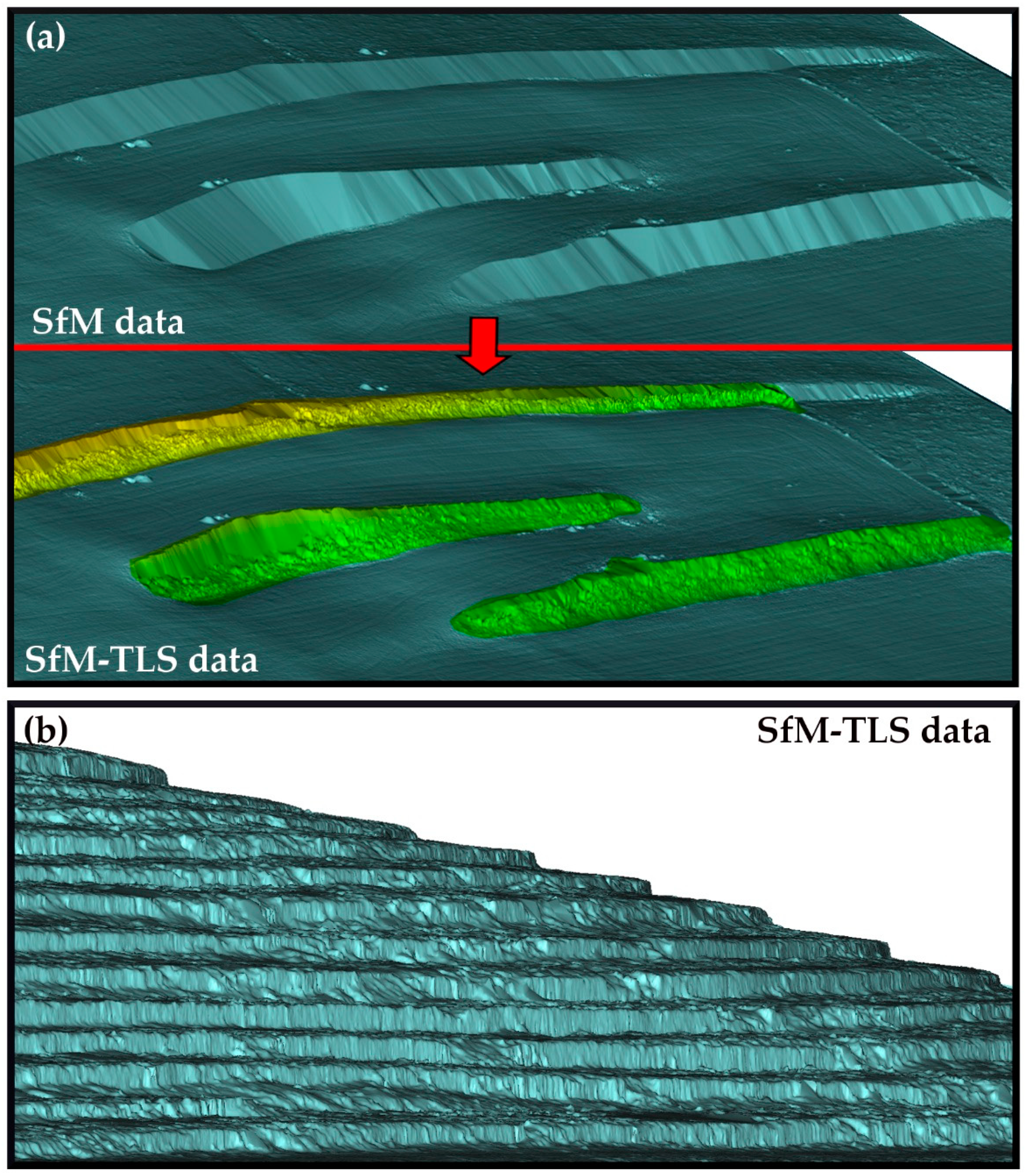
4.3. Data Fusion
4.4. DTM Error Assesment
5. Conclusions
Author Contributions
Funding
Acknowledgments
Conflicts of Interest
References
- Hengl, T.; Reuter, H.I. Geomorphometry: Concepts, Software, Applications, 1st ed.; Elsevier Science: Amsterdam, The Netherlands, 2009. [Google Scholar]
- Tarolli, P. High-resolution topography for understanding Earth surface processes: Opportunities and challenges. Geomorphology 2014, 216, 295–312. [Google Scholar] [CrossRef]
- Glennie, C.L.; Carter, W.E.; Shrestha, R.L.; Dietrich, W.E. Geodetic imaging with airborne LiDAR: The Earth’s surface revealed. Rep. Prog. Phys. 2013, 76, 86801. [Google Scholar] [CrossRef] [PubMed]
- Passalacqua, P.; Hillier, J.K.; Tarolli, P. Innovative analysis and use of high-resolution DTMs for quantitative interrogation of Earth-surface processes. Earth Surf. Process. Landf. 2014, 39, 1400–1403. [Google Scholar] [CrossRef] [Green Version]
- Passalacqua, P.; Belmont, P.; Staley, D.M.; Simley, J.D.; Arrowsmith, J.R.; Bode, C.A.; Crosby, C.; Delong, S.B.; Glenn, N.F.; Kelly, S.A.; et al. Analyzing high resolution topography for advancing the understanding of mass and energy transfer through landscapes: A review. Earth Sci. Rev. 2015, 148, 174–193. [Google Scholar] [CrossRef] [Green Version]
- Bangen, S.; Wheaton, J.M.; Bouwes, N.; Bouwes, B.; Jordan, C. A methodological intercomparison of topographic survey techniques for characterizing wadeable streams and rivers. Geomorphology 2014, 206, 343–361. [Google Scholar] [CrossRef]
- James, L.A.; Watson, D.G.; Hansen, W.F.; James, L.A. Using LiDAR data to map gullies and headwater streams under forest canopy: South Carolina, USA. Catena 2007, 71, 132–144. [Google Scholar] [CrossRef]
- Cavalli, M.; Marchi, L. Characterisation of the surface morphology of an alpine alluvial fan using airborne LiDAR. Nat. Hazards Earth Syst. Sci. 2008, 8, 323–333. [Google Scholar] [CrossRef]
- Sofia, G.; Pirotti, F.; Tarolli, P. Variations in multiscale curvature distribution and signatures of LiDAR DTM errors. Earth Surf. Process. Landf. 2013, 38, 1116–1134. [Google Scholar] [CrossRef]
- Roering, J.J.; Mackey, B.H.; Marshall, J.A.; Sweeney, K.E.; Deligne, N.; Booth, A.M.; Handwerger, A.L.; Cerovski-Darriau, C. ‘You are HERE’: Connecting the dots with airborne lidar for geomorphic fieldwork. Geomorphology 2013, 200, 172–183. [Google Scholar] [CrossRef]
- Pfeifer, N.; Mandlburger, G.; Otepka, J.; Karel, W. OPALS—A framework for Airborne Laser Scanning data analysis. Comput. Environ. Urban. Syst. 2014, 45, 125–136. [Google Scholar] [CrossRef]
- Schwendel, A.C.; Milan, D.J. Terrestrial structure-from-motion: Spatial error analysis of roughness and morphology. Geomorphology 2020, 350, 106883. [Google Scholar] [CrossRef]
- Lobb, M.; Brown, A.G.; Leyland, J.; Bernard, V.; Daire, M.Y.; Langouët, L. An estuarine tide-scape of production: Terrestrial laser scanning (TLS) of fixed fishing structures and a tidal mill in the Léguer Estuary, Brittany, France. Antiquity 2018, in press. [Google Scholar]
- Tong, X.; Liu, X.; Chen, P.; Liu, S.; Luan, K.; Li, L.; Liu, S.; Liu, X.; Xie, H.; Jin, Y.; et al. Integration of UAV-Based Photogrammetry and Terrestrial Laser Scanning for the Three-Dimensional Mapping and Monitoring of Open-Pit Mine Areas. Remote Sens. 2015, 7, 6635–6662. [Google Scholar] [CrossRef] [Green Version]
- Westoby, M.; Brasington, J.; Glasser, N.F.; Hambrey, M.; Reynolds, J. ‘Structure-from-Motion’ photogrammetry: A low-cost, effective tool for geoscience applications. Geomorphology 2012, 179, 300–314. [Google Scholar] [CrossRef] [Green Version]
- Carrivick, J.L.; Smith, M.W.; Quincey, D. Structure from Motion in the Geosci; John Wiley & Sons: Hoboken, NJ, USA, 2016. [Google Scholar]
- James, M.R.; Chandler, J.H.; Eltner, A.; Fraser, C.; Miller, P.E.; Mills, J.P.; Noble, T.; Robson, S.; Lane, S.N. Guidelines on the use of structure-from-motion photogrammetry in geomorphic research. Earth Surf. Process. Landf. 2019, 44, 2081–2084. [Google Scholar] [CrossRef]
- Bastonero, P.; Donadio, E.; Chiabrando, F.; Spanò, A. Fusion of 3D models derived from TLS and image-based techniques for CH enhanced documentation. ISPRS Ann. Photogramm. Remote Sens. Spat. Inf. Sci. 2014, 2, 73–80. [Google Scholar] [CrossRef] [Green Version]
- Ramos, M.M.; Remondino, F. Data fusion in Cultural Heritage—A Review. ISPRS Int. Arch. Photogramm. Remote Sens. Spat. Inf. Sci. 2015, 40, 359–363. [Google Scholar] [CrossRef] [Green Version]
- Tarolli, P.; Sofia, G.; Calligaro, S.; Prosdocimi, M.; Preti, F.; Fontana, G.D. Vineyards in Terraced Landscapes: New Opportunities from Lidar Data. Land Degrad. Dev. 2014, 26, 92–102. [Google Scholar] [CrossRef]
- Forlani, G.; Diotri, F.; Di Cella, U.M.; Roncella, R. Indirect UAV Strip Georeferencing by on-Board GNSS Data under Poor Satellite Coverage. Remote Sens. 2019, 11, 1765. [Google Scholar] [CrossRef] [Green Version]
- Sofia, G.; Roder, G.; Fontana, G.D.; Tarolli, P. Flood dynamics in urbanised landscapes: 100 years of climate and humans’ interaction. Sci. Rep. 2017, 7, 40527. [Google Scholar] [CrossRef]
- Brown, A.G.; Walsh, K.; Fallu, D.; Cucchiaro, S.; Tarolli, P. Global agricultural terraces and lynchets: From archaeological theory to heritage management. Submitted to World Archaeology.
- Lesschen, J.P.; Cammeraat, E.; Nieman, T. Erosion and terrace failure due to agricultural land abandonment in a semi-arid environment. Earth Surf. Process. Landf. 2008, 33, 1574–1584. [Google Scholar] [CrossRef]
- Tarolli, P.; Preti, F.; Romano, N. Terraced landscapes: From an old best practice to a potential hazard for soil degradation due to land abandonment. Anthropocene 2014, 6, 10–25. [Google Scholar] [CrossRef]
- Tarolli, P. Agricultural Terraces Special Issue Preface. Land Degrad. Dev. 2018, 29, 3544–3548. [Google Scholar] [CrossRef]
- Pijl, A.; Tosoni, M.; Roder, G.; Sofia, G.; Tarolli, P.; Pijl, A. Design of Terrace Drainage Networks Using UAV-Based High-Resolution Topographic Data. Water 2019, 11, 814. [Google Scholar] [CrossRef] [Green Version]
- Tarolli, P.; Straffelini, E. Agriculture in Hilly and Mountainous Landscapes: Threats, Monitoring and Sustainable Management. Geogr. Sustain. 2020, 1, 70–76. [Google Scholar] [CrossRef]
- Cucchiaro, S.; Fallu, D.J.; Zhao, P.; Waddington, C.; Cockcroft, D.; Tarolli, P.; Brown, A.G. SfM photogrammetry for GeoArchaeology. Dev. Earth Surf. Process. 2020, 23, 183–205. [Google Scholar] [CrossRef]
- Zieher, T.; Toschi, I.; Remondino, F.; Rutzinger, M.; Kofler, C.; Mejia-Aguilar, A.; Schlögel, R. Sensor- and Scene-Guided Integration of Tls and Photogrammetric Point Clouds for Landslide Monitoring. ISPRS Int. Arch. Photogramm. Remote Sens. Spat. Inf. Sci. 2018, 42, 1243–1250. [Google Scholar] [CrossRef] [Green Version]
- Klein, L.A. Sensor and Data Fusion: A Tool for Information Assessment and Decision Making, 2nd ed.; SPIE Press: Bellingham, WA, USA, 2004. [Google Scholar]
- Xu, Z.; Wu, L.; Shen, Y.; Li, F.; Wang, Q.; Wang, R. Tridimensional Reconstruction Applied to Cultural Heritage with the Use of Camera-Equipped UAV and Terrestrial Laser Scanner. Remote Sens. 2014, 6, 10413–10434. [Google Scholar] [CrossRef] [Green Version]
- Balletti, C.; Guerra, F.; Scocca, V.; Gottardi, C. 3D Integrated Methodologies for the Documentation and the Virtual Reconstruction of an Archaeological Site. ISPRS Int. Arch. Photogramm. Remote Sens. Spat. Inf. Sci. 2015, 40, 215–222. [Google Scholar] [CrossRef] [Green Version]
- Chiabrando, F.; Di Pietra, V.; Lingua, A.; Maschio, P.; Noardo, F.; Sammartano, G.; Spanò, A. TLS models generation assisted By UAV survey. Int. Arch. Photogramm. Remote Sens. Spat. Inf. Sci. ISPRS Arch. 2016, 41, 413–420. [Google Scholar]
- Chatzistamatis, S.; Kalaitzis, P.; Chaidas, K.; Chatzitheodorou, C.; Papadopoulou, E.E.; Tataris, G.; Soulakellis, N. Fusion of Tls and Uav Photogrammetry Data for Post-Earthquake 3d Modeling of a Cultural Heritage Church. ISPRS Int. Arch. Photogramm. Remote Sens. Spat. Inf. Sci. 2018, 42, 143–150. [Google Scholar] [CrossRef] [Green Version]
- Luhmann, T.; Chizhova, M.; Gorkovchuk, D.; Hastedt, H.; Chachava, N.; Lekveishvili, N. Combination of Terrestrial Laserscanning, Uav and Close-Range Photogrammetry for 3d Reconstruction of Complex Churches in Georgia. ISPRS Int. Arch. Photogramm. Remote Sens. Spat. Inf. Sci. 2019, 42, 753–761. [Google Scholar] [CrossRef] [Green Version]
- Eltner, A.; Kaiser, A.; Castillo, C.; Rock, G.; Neugirg, F.; Abellán, A. Image-based surface reconstruction in geomorphometry—Merits, limits and developments. Earth Surf. Dyn. 2016, 4, 359–389. [Google Scholar] [CrossRef] [Green Version]
- Tilly, N.; Kelterbaum, D.; Zeese, R. Geomorphological mapping with terrestrial laser scanning and uav-based imaging. Int. Arch. Photogramm. Remote Sens. Spat. Inf. Sci. ISPRS Arch. 2016, 41, 591–597. [Google Scholar] [CrossRef]
- Šašak, J.; Gallay, M.; Kaňuk, J.; Hofierka, J.; Minár, J. Combined Use of Terrestrial Laser Scanning and UAV Photogrammetry in Mapping Alpine Terrain. Remote Sens. 2019, 11, 2154. [Google Scholar] [CrossRef] [Green Version]
- Wu, B.; Tang, S. Review of geometric fusion of remote sensing imagery and laser scanning data. Int. J. Image Data Fusion 2015, 6, 97–114. [Google Scholar] [CrossRef]
- Brandolini, P.; Cevasco, A.; Capolongo, D.; Pepe, G.; Lovergine, F.; Del Monte, M. Response of Terraced Slopes to a Very Intense Rainfall Event and Relationships with Land Abandonment: A Case Study from Cinque Terre (Italy). Land Degrad. Dev. 2017, 29, 630–642. [Google Scholar] [CrossRef]
- Camera, C.; Djuma, H.; Bruggeman, A.; Zoumides, C.; Eliades, M.; Charalambous, K. Catena Quantifying the e ff ectiveness of mountain terraces on soil erosion protection with sediment traps and dry-stone wall laser scans. Catena 2018, 171, 251–264. [Google Scholar] [CrossRef]
- Calsamiglia, A.; Fortesa, J.; García-Comendador, J.; Lucas-Borja, M.E.; Calvo-Cases, A.; Bertos, J.E. Spatial patterns of sediment connectivity in terraced lands: Anthropogenic controls of catchment sensitivity. Land Degrad. Dev. 2017, 29, 1198–1210. [Google Scholar] [CrossRef]
- Brodu, N.; Lague, D. 3D terrestrial lidar data classification of complex natural scenes using a multi-scale dimensionality criterion: Applications in geomorphology. ISPRS J. Photogramm. Remote Sens. 2012, 68, 121–134. [Google Scholar] [CrossRef] [Green Version]
- Guarnieri, A.; Vettore, A.; Pirotti, F.; Menenti, M.; Marani, M. Retrieval of small-relief marsh morphology from Terrestrial Laser Scanner, optimal spatial filtering, and laser return intensity. Geomorphology 2009, 113, 12–20. [Google Scholar] [CrossRef]
- Medjkane, M.; Maquaire, O.; Costa, S.; Roulland, T.; Letortu, P.; Fauchard, C.; Antoine, R.; Davidson, R. High-resolution monitoring of complex coastal morphology changes: Cross-efficiency of SfM and TLS-based survey (Vaches-Noires cliffs, Normandy, France). Landslides 2018, 15, 1097–1108. [Google Scholar] [CrossRef]
- Rossi, P.; Mancini, F.; Dubbini, M.; Mazzone, F.; Capra, A. Combining nadir and oblique UAV imagery to reconstruct quarry topography: Methodology and feasibility analysis. Eur. J. Remote Sens. 2017, 50, 211–221. [Google Scholar] [CrossRef]
- Li, W.; Wang, C.; Zai, D.; Huang, P.; Liu, W.; Wen, C.; Li, J. A Volumetric Fusing Method for TLS and SFM Point Clouds. IEEE J. Sel. Top. Appl. Earth Obs. Remote Sens. 2018, 11, 3349–3357. [Google Scholar] [CrossRef]
- Colomina, I.; Molina, P. Unmanned aerial systems for photogrammetry and remote sensing: A review. ISPRS J. Photogramm. Remote Sens. 2014, 92, 79–97. [Google Scholar] [CrossRef] [Green Version]
- Manfreda, S.; McCabe, M.; Miller, P.; Lucas, R.; Madrigal, V.P.; Mallinis, G.; Ben Dor, E.; Helman, D.; Estes, L.D.; Ciraolo, G.; et al. On the Use of Unmanned Aerial Systems for Environmental Monitoring. Remote Sens. 2018, 10, 641. [Google Scholar] [CrossRef] [Green Version]
- Tmušić, G.; Manfreda, S.; Aasen, H.; James, M.R.; Gonçalves, G.; Ben Dor, E.; Brook, A.; Polinova, M.; Arranz, J.J.; Mészáros, J.; et al. Current Practices in UAS-based Environmental Monitoring. Remote Sens. 2020, 12, 1001. [Google Scholar] [CrossRef] [Green Version]
- Cucchiaro, S.; Maset, E.; Fusiello, A.; Cazorzi, F. 4d-Sfm Photogrammetry for Monitoring Sediment Dynamics in a Debris-Flow Catchment: Software Testing and Results Comparison. ISPRS Int. Arch. Photogramm. Remote Sens. Spat. Inf. Sci. 2018, 42, 281–288. [Google Scholar] [CrossRef] [Green Version]
- Niethammer, U.; James, M.R.; Rothmund, S.; Travelletti, J.; Joswig, M. UAV-based remote sensing of the Super-Sauze landslide: Evaluation and results. Eng. Geol. 2012, 128, 2–11. [Google Scholar] [CrossRef]
- Smith, M.W.; Carrivick, J.L.; Quincey, D. Structure from motion photogrammetry in physical geography. Prog. Phys. Geogr. Earth Environ. 2015, 40, 247–275. [Google Scholar] [CrossRef]
- Crema, S.; Llena, M.; Calsamiglia, A.; Bertos, J.E.; Marchi, L.; Vericat, D.; Cavalli, M. Can inpainting improve digital terrain analysis? Comparing techniques for void filling, surface reconstruction and geomorphometric analyses. Earth Surf. Process. Landf. 2020, 45, 736–755. [Google Scholar] [CrossRef]
- Carbonneau, P.; Dietrich, J.T. Cost-effective non-metric photogrammetry from consumer-grade sUAS: Implications for direct georeferencing of structure from motion photogrammetry. Earth Surf. Process. Landf. 2016, 42, 473–486. [Google Scholar] [CrossRef] [Green Version]
- Benassi, F.; Dall’Asta, E.; Diotri, F.; Forlani, G.; Di Cella, U.M.; Roncella, R.; Santise, M. Testing Accuracy and Repeatability of UAV Blocks Oriented with GNSS-Supported Aerial Triangulation. Remote Sens. 2017, 9, 172. [Google Scholar] [CrossRef] [Green Version]
- James, M.R.; Robson, S.; D’Oleire-Oltmanns, S.; Niethammer, U. Optimising UAV topographic surveys processed with structure-from-motion: Ground control quality, quantity and bundle adjustment. Geomorphology 2017, 280, 51–66. [Google Scholar] [CrossRef] [Green Version]
- Forlani, G.; Dall’Asta, E.; Diotri, F.; Di Cella, U.M.; Roncella, R.; Santise, M. Quality Assessment of DSMs Produced from UAV Flights Georeferenced with On-Board RTK Positioning. Remote Sens. 2018, 10, 311. [Google Scholar] [CrossRef] [Green Version]
- Tomaštík, J.; Mokroš, M.; Surový, P.; Grznárová, A.; Merganič, J. UAV RTK/PPK method-An optimal solution for mapping inaccessible forested areas? Remote Sens. 2019, 11, 721. [Google Scholar] [CrossRef] [Green Version]
- Pfeifer, N.; Glira, P.; Briese, C. Direct georeferencing with on board navigation components of light weight uav platforms. ISPRS Int. Arch. Photogramm. Remote Sens. Spat. Inf. Sci. 2012, 39, 487–492. [Google Scholar] [CrossRef] [Green Version]
- Turner, D.; Lucieer, A.; Wallace, L.O. Direct Georeferencing of Ultrahigh-Resolution UAV Imagery. IEEE Trans. Geosci. Remote Sens. 2014, 52, 2738–2745. [Google Scholar] [CrossRef]
- Stöcker, C.; Nex, F.; Koeva, M.; Gerke, M. QUALITY ASSESSMENT OF COMBINED IMU/GNSS DATA FOR DIRECT GEOREFERENCING IN THE CONTEXT OF UAV-BASED MAPPING. ISPRS Int. Arch. Photogramm. Remote Sens. Spat. Inf. Sci. 2017, 42, 355–361. [Google Scholar] [CrossRef] [Green Version]
- Padró, J.-C.; Muñoz, F.-J.; Planas, J.; Pons, X. Comparison of four UAV georeferencing methods for environmental monitoring purposes focusing on the combined use with airborne and satellite remote sensing platforms. Int. J. Appl. Earth Obs. Geoinf. 2019, 75, 130–140. [Google Scholar] [CrossRef]
- Zhang, H.; Aldana-Jague, E.; Clapuyt, F.; Wilken, F.; Vanacker, V.; Van Oost, K. Evaluating the Potential of PPK Direct Georeferencing for UAV-SfM Photogrammetry and Precise Topographic Mapping. Earth Surf. Dyn. Discuss. 2019, 1–34. [Google Scholar] [CrossRef]
- Azmi, M.A.A.M.; Abbas, M.A.; Zainuddin, K.; Mustafar, M.A.; Zainal, M.Z.; Majid, Z.; Idris, K.M.; Ariff, M.F.M.; Luh, L.C.; Aspuri, A. 3D Data Fusion Using Unmanned Aerial Vehicle (UAV) Photogrammetry and Terrestrial Laser Scanner (TLS). In Proceedings of the Second International Conference on the Future of ASEAN (ICoFA) 2017—Volume 2; Springer Science and Business Media LLC: Berlin, Germany, 2018. [Google Scholar]
- Prosdocimi, M.; Calligaro, S.; Sofia, G.; Fontana, G.D.; Tarolli, P. Bank erosion in agricultural drainage networks: New challenges from structure-from-motion photogrammetry for post-event analysis. Earth Surf. Process. Landf. 2015, 40, 1891–1906. [Google Scholar] [CrossRef]
- Smith, M.W.; Vericat, D. From experimental plots to experimental landscapes: Topography, erosion and deposition in sub-humid badlands from Structure-from-Motion photogrammetry. Earth Surf. Process. Landf. 2015, 40, 1656–1671. [Google Scholar] [CrossRef] [Green Version]
- Clapuyt, F.; Vanacker, V.; Van Oost, K. Reproducibility of UAV-based earth topography reconstructions based on Structure-from-Motion algorithms. Geomorphology 2016, 260, 4–15. [Google Scholar] [CrossRef]
- Glendell, M.; McShane, G.; Farrow, L.; James, M.R.; Quinton, J.N.; Anderson, K.; Evans, M.; Benaud, P.; Rawlins, B.; Morgan, D.; et al. Testing the utility of structure-from-motion photogrammetry reconstructions using small unmanned aerial vehicles and ground photography to estimate the extent of upland soil erosion. Earth Surf. Process. Landf. 2017, 42, 1860–1871. [Google Scholar] [CrossRef]
- Cucchiaro, S.; Maset, E.; Cavalli, M.; Crema, S.; Marchi, L.; Beinat, A.; Cazorzi, F. How does co-registration affect geomorphic change estimates in multi-temporal surveys? GIScience Remote Sens. 2020, 45, 1–22. [Google Scholar] [CrossRef]
- Bornaz, L.; Lingua, A.; Rinaudo, F. Multiple scan registration in LIDAR close range applications. Int. Arch. Photogram. Rem. Sens. Spat. Inform. Sci. 2003, 34, 72–77. [Google Scholar]
- Nyssen, J.; Debever, M.; Jean, P.; Deckers, J. Lynchets in eastern Belgium—A geomorphic feature resulting from non-mechanised crop farming. Catena 2014, 121, 164–175. [Google Scholar] [CrossRef] [Green Version]
- Sanz-Ablanedo, E.; Chandler, J.; Rodríguez-Pérez, J.R.; Ordóñez, C. Accuracy of Unmanned Aerial Vehicle (UAV) and SfM Photogrammetry Survey as a Function of the Number and Location of Ground Control Points Used. Remote Sens. 2018, 10, 1606. [Google Scholar] [CrossRef] [Green Version]
- Tonkin, T.; Midgley, N. Ground-Control Networks for Image Based Surface Reconstruction: An Investigation of Optimum Survey Designs Using UAV Derived Imagery and Structure-from-Motion Photogrammetry. Remote Sens. 2016, 8, 786. [Google Scholar] [CrossRef] [Green Version]
- Marteau, B.; Vericat, D.; Gibbins, C.; Batalla, R.J.; Green, D.R. Application of Structure-from-Motion photogrammetry to river restoration. Earth Surf. Process. Landf. 2016, 42, 503–515. [Google Scholar] [CrossRef] [Green Version]
- Cucchiaro, S.; Cavalli, M.; Vericat, D.; Crema, S.; Llena, M.; Beinat, A.; Marchi, L.; Cazorzi, F. Monitoring topographic changes through 4D-structure-from-motion photogrammetry: Application to a debris-flow channel. Environ. Earth Sci. 2018, 77, 632. [Google Scholar] [CrossRef]
- Guarnieri, A.; Fissore, F.; Masiero, A.; Di Donna, A.; Coppa, U.; Vettore, A. From Survey to Fem Analysis for Documentation of Built Heritage: The Case Study of Villa Revedin-Bolasco. ISPRS Int. Arch. Photogramm. Remote Sens. Spat. Inf. Sci. 2017, 42, 527–533. [Google Scholar] [CrossRef] [Green Version]
- James, M.R.; Robson, S. Straightforward reconstruction of 3D surfaces and topography with a camera: Accuracy and geoscience application. J. Geophys. Res. Space Phys. 2012, 117, 1–17. [Google Scholar] [CrossRef] [Green Version]
- Harwin, S.; Lucieer, A.; Osborn, J. The Impact of the Calibration Method on the Accuracy of Point Clouds Derived Using Unmanned Aerial Vehicle Multi-View Stereopsis. Remote Sens. 2015, 7, 11933–11953. [Google Scholar] [CrossRef] [Green Version]
- Granshaw, S.I. Bundle adjustment methods in engineering photogrammetry. Photogramm. Rec. 2006, 10, 181–207. [Google Scholar] [CrossRef]
- Woodget, A.; Carbonneau, P.E.; Visser, F.; Maddock, I. Quantifying submerged fluvial topography using hyperspatial resolution UAS imagery and structure from motion photogrammetry. Earth Surf. Process. Landf. 2014, 40, 47–64. [Google Scholar] [CrossRef] [Green Version]
- Piermattei, L.; Carturan, L.; Guarnieri, A. Use of terrestrial photogrammetry based on structure-from-motion for mass balance estimation of a small glacier in the Italian alps. Earth Surf. Process. Landf. 2015, 40, 1791–1802. [Google Scholar] [CrossRef]
- Zhang, J.; Hu, J.; Lian, J.; Fan, Z.; Ouyang, X.; Ye, W. Seeing the forest from drones: Testing the potential of lightweight drones as a tool for long-term forest monitoring. Boil. Conserv. 2016, 198, 60–69. [Google Scholar] [CrossRef]
- Zeybek, M.; Şanlıoğlu, I. Point cloud filtering on UAV based point cloud. Measurement 2019, 133, 99–111. [Google Scholar] [CrossRef]
- Lague, D.; Brodu, N.; Leroux, J. Accurate 3D comparison of complex topography with terrestrial laser scanner: Application to the Rangitikei canyon (N-Z). ISPRS J. Photogramm. Remote Sens. 2013, 82, 10–26. [Google Scholar] [CrossRef] [Green Version]
- Chen, Y.; Medioni, G. Object modelling by registration of multiple range images. Image Vis. Comput. 1992, 10, 145–155. [Google Scholar] [CrossRef]
- Besl, P.; McKay, H. A method for registration of 3-D shapes. IEEE Trans. Pattern Anal. Mach. Intell. 1992, 14, 239–256. [Google Scholar] [CrossRef]
- Guarnieri, A.; Remondino, F.; Vettore, A. Digital photogrammetry and TLS data fusion applied to Cultural Heritage 3D modeling. Int. Arch. Photogramm. Remote Sens. Spat. Inf. Sci. 2006, 36, 1–6. [Google Scholar]
- Zang, Y.; Yang, B.; Li, J.; Guan, H. An Accurate TLS and UAV Image Point Clouds Registration Method for Deformation Detection of Chaotic Hillside Areas. Remote Sens. 2019, 11, 647. [Google Scholar] [CrossRef] [Green Version]
- Micheletti, N.; Chandler, J.; Lane, S.N. Investigating the geomorphological potential of freely available and accessible structure-from-motion photogrammetry using a smartphone. Earth Surf. Process. Landf. 2014, 40, 473–486. [Google Scholar] [CrossRef] [Green Version]
- Cucchiaro, S.; Cavalli, M.; Vericat, D.; Crema, S.; Llena, M.; Beinat, A.; Marchi, L.; Cazorzi, F. Geomorphic effectiveness of check dams in a debris-flow catchment using multi-temporal topographic surveys. Catena 2019, 174, 73–83. [Google Scholar] [CrossRef]
- Parente, L.; Chandler, J.; Dixon, N. Optimising the quality of an SfM-MVS slope monitoring system using fixed cameras. Photogramm. Rec. 2019, 34, 408–427. [Google Scholar] [CrossRef]
- Wheaton, J.M.; Brasington, J.; Darby, S.E.; Sear, D.A. Accounting for uncertainty in DEMs from repeat topographic surveys: Improved sediment budgets. Earth Surf. Process. Landf. 2009, 35, 136–156. [Google Scholar] [CrossRef]
- Javernick, L.; Brasington, J.; Caruso, B. Modeling the topography of shallow braided rivers using Structure-from-Motion photogrammetry. Geomorphology 2014, 213, 166–182. [Google Scholar] [CrossRef]
- Vericat, D.; Smith, M.W.; Brasington, J. Patterns of topographic change in sub-humid badlands determined by high resolution multi-temporal topographic surveys. Catena 2014, 120, 164–176. [Google Scholar] [CrossRef]
- Brasington, J.; Vericat, D.; Rychkov, I. Modeling river bed morphology, roughness, and surface sedimentology using high resolution terrestrial laser scanning. Water Resour. Res. 2012, 48, 1–18. [Google Scholar] [CrossRef] [Green Version]
- Heritage, G.L.; Milan, D.J.; Large, A.R.; Fuller, I. Influence of survey strategy and interpolation model on DEM quality. Geomorphology 2009, 112, 334–344. [Google Scholar] [CrossRef]
- Milan, D.J.; Heritage, G.L.; Large, A.R.; Fuller, I. Filtering spatial error from DEMs: Implications for morphological change estimation. Geomorphology 2011, 125, 160–171. [Google Scholar] [CrossRef]
- Höhle, J.; Höhle, M. ISPRS Journal of Photogrammetry and Remote Sensing Accuracy assessment of digital elevation models by means of robust statistical methods. ISPRS J. Photogramm. Remote Sens. 2009, 64, 398–406. [Google Scholar] [CrossRef] [Green Version]
- Gonçalves, G.; Pérez, J.A.; Duarte, J. Accuracy and effectiveness of low cost UASs and open source photogrammetric software for foredunes mapping. Int. J. Remote Sens. 2018, 39, 5059–5077. [Google Scholar] [CrossRef]
- Remondino, F.; Nocerino, E.; Toschi, I.; Menna, F. A critical review of automated photogrammetric processing of large datasets. ISPRS Int. Arch. Photogramm. Remote Sens. Spat. Inf. Sci. 2017, 42, 591–599. [Google Scholar] [CrossRef] [Green Version]
- Turner, D.; Lucieer, A.; Watson, C.S. An Automated Technique for Generating Georectified Mosaics from Ultra-High Resolution Unmanned Aerial Vehicle (UAV) Imagery, Based on Structure from Motion (SfM) Point Clouds. Remote Sens. 2012, 4, 1392–1410. [Google Scholar] [CrossRef] [Green Version]
- Nolan, M.; Larsen, C.F.; Sturm, M. Mapping snow-depth from manned-aircraft on landscape scales at centimeter resolution using Structure-from-Motion photogrammetry. Cryosphere Discuss. 2015, 9, 333–381. [Google Scholar] [CrossRef]
- Shahbazi, M.; Sohn, G.; Théau, J.; Ménard, P. Development and Evaluation of a UAV-Photogrammetry System for Precise 3D Environmental Modeling. Sensors 2015, 15, 27493–27524. [Google Scholar] [CrossRef] [Green Version]
- Gerke, M. Accuracy Analysis of Photogrammetric UAV Image Blocks: Influence of Onboard RTK-GNSS and Cross Flight Patterns. Photogramm. Fernerkund. Geoinf. 2016, 2016, 17–30. [Google Scholar] [CrossRef] [Green Version]
- Eltner, A.; Sofia, G. Structure from motion photogrammetric technique. Dev. Earth Surf. Process. 2020, 23, 1–24. [Google Scholar] [CrossRef]
- Jozkow, G.; Toth, C. Georeferencing experiments with UAS imagery. ISPRS Ann. Photogramm. Remote Sens. Spat. Inf. Sci. 2014, 25, 25–29. [Google Scholar] [CrossRef] [Green Version]
- Benjamin, A.R.; O’Brien, D.; Barnes, G.; Wilkinson, B.E.; Volkmann, W. Improving Data Acquisition Efficiency: Systematic Accuracy Evaluation of GNSS-Assisted Aerial Triangulation in UAS Operations. J. Surv. Eng. 2020, 146, 05019006. [Google Scholar] [CrossRef]
- James, M.R.; Robson, S.; Smith, M.W. 3-D uncertainty-based topographic change detection with structure-from-motion photogrammetry: Precision maps for ground control and directly georeferenced surveys. Earth Surf. Process. Landf. 2017, 42, 1769–1788. [Google Scholar] [CrossRef]
- Hugenholtz, C.; Brown, O.; Walker, J.; Barchyn, T.E.; Nesbit, P.; Kucharczyk, M.; Myshak, S. Spatial Accuracy of UAV-Derived Orthoimagery and Topography: Comparing Photogrammetric Models Processed with Direct Geo-Referencing and Ground Control Points. Geomatica 2016, 70, 21–30. [Google Scholar] [CrossRef]
- Zhou, Y.; Rupnik, E.; Faure, P.-H.; Pierrot-Deseilligny, M. GNSS-Assisted Integrated Sensor Orientation with Sensor Pre-Calibration for Accurate Corridor Mapping †. Sensors 2018, 18, 2783. [Google Scholar] [CrossRef] [Green Version]
- Gabrlik, P.; La Cour-Harbo, A.; Kalvodova, P.; Zalud, L.; Janata, P. Calibration and accuracy assessment in a direct georeferencing system for UAS photogrammetry. Int. J. Remote Sens. 2018, 39, 4931–4959. [Google Scholar] [CrossRef] [Green Version]
- James, M.R.; Robson, S. Mitigating systematic error in topographic models derived from UAV and ground-based image networks. Earth Surf. Process. Landf. 2014, 39, 1413–1420. [Google Scholar] [CrossRef] [Green Version]
- Bemis, S.; Micklethwaite, S.; Turner, D.; James, M.R.; Akciz, S.O.; Thiele, S.; Bangash, H.A. Ground-based and UAV-Based photogrammetry: A multi-scale, high-resolution mapping tool for structural geology and paleoseismology. J. Struct. Geol. 2014, 69, 163–178. [Google Scholar] [CrossRef]
- Cook, K. An evaluation of the effectiveness of low-cost UAVs and structure from motion for geomorphic change detection. Geomorphology 2017, 278, 195–208. [Google Scholar] [CrossRef]
- Pfeiffer, J.; Zieher, T.; Bremer, M.; Wichmann, V.; Rutzinger, M. Derivation of Three-Dimensional Displacement Vectors from Multi-Temporal Long-Range Terrestrial Laser Scanning at the Reissenschuh Landslide (Tyrol, Austria). Remote Sens. 2018, 10, 1688. [Google Scholar] [CrossRef] [Green Version]
- Beinat, A.; Crosilla, F. Generalized Procrustes Analysis for Size and Shape 3-D Object Reconstructions. Optical 2001, 345–353. [Google Scholar]
- James, M.R.; Quinton, J.N. Ultra-rapid topographic surveying for complex environments: The hand-held mobile laser scanner (HMLS). Earth Surf. Process. Landf. 2013, 39, 138–142. [Google Scholar] [CrossRef] [Green Version]
- Nahon, A.; Molina, P.; Blázquez, M.; Simeon, J.; Capo, S.; Ferrero, C. Corridor Mapping of Sandy Coastal Foredunes with UAS Photogrammetry and Mobile Laser Scanning. Remote Sens. 2019, 11, 1352. [Google Scholar] [CrossRef] [Green Version]
- Torresan, C.; Berton, A.; Carotenuto, F.; Chiavetta, U.; Miglietta, F.; Zaldei, A.; Gioli, B. Development and Performance Assessment of a Low-Cost UAV Laser Scanner System (LasUAV). Remote Sens. 2018, 10, 1094. [Google Scholar] [CrossRef] [Green Version]
- Brasington, J.; Langham, J.; Rumsby, B. Methodological sensitivity of morphometric estimates of coarse fluvial sediment transport. Geomorphology 2003, 53, 299–316. [Google Scholar] [CrossRef]
- Lane, S.N.; Westaway, R.M.; Hicks, D.M. Estimation of erosion and deposition volumes in a large, gravel-bed, braided river using synoptic remote sensing. Earth Surf. Process. Landf. 2003, 28, 249–271. [Google Scholar] [CrossRef]
- Chaplot, V.; Darboux, F.; Bourennane, H.; Leguédois, S.; Silvera, N.; Phachomphon, K. Accuracy of interpolation techniques for the derivation of digital elevation models in relation to landform types and data density. Geomorphology 2006, 77, 126–141. [Google Scholar] [CrossRef]
- Schwendel, A.C.; Fuller, I.; Death, R.G. Assessing DEM interpolation methods for effective representation of upland stream morphology for rapid appraisal of bed stability. River Res. Appl. 2010, 28, 567–584. [Google Scholar] [CrossRef] [Green Version]
- Wang, B.; Shi, W.; Liu, E. Robust methods for assessing the accuracy of linear interpolated DEM. Int. J. Appl. Earth Obs. Geoinf. 2015, 34, 198–206. [Google Scholar] [CrossRef]
- Tarolli, P.; Cao, W.; Sofia, G.; Evans, D.; Ellis, E.C. From features to fingerprints: A general diagnostic framework for anthropogenic geomorphology. Prog. Phys. Geogr. Earth Environ. 2019, 43, 95–128. [Google Scholar] [CrossRef] [Green Version]


| Study Area | Area Covered (ha) | Number of Images | Flight Height (m) | GSD (m) | Number of GCPs (CPs) 1 | GNSS Positional Accuracy (X, Y—Z) (m) |
|---|---|---|---|---|---|---|
| Belgium | 18 | 1219 | 20–45 | 0.005–0.015 | 40 (13) | <0.05 |
| Italy | 3.5 | 632 | 25–35 | 0.006–0.008 | 56 (18) | 0.03–0.04 |
| Study Area | Number of Scans | Mean Distance between Scans (m) | Accuracy (m) | Maximum Range Mode (m) | Scan Rate (Points/s) | Image Resolution (Mpixels) | Number of Targets |
|---|---|---|---|---|---|---|---|
| Belgium | 7 | 70 | 1.6 mm@10 | 120 | 1,000,000 | 4 | 20 |
| Italy | 6 | 65 | 1.6 mm@10 | 270–570 1 | 250,000–500,000 1 | 4 | 16 |
| Solution Type | Accuracy | Precision | Registration | ||||||
|---|---|---|---|---|---|---|---|---|---|
| MAE (m) | RMSE3D 1 (m) | SDE (m) | RMSE3D 1 (m) | Cameras 2 (m) | |||||
| X | Y | Z | CPs | X | Y | Z | GCPs | ||
| Italy | |||||||||
| GCP | 0.013 | 0.014 | 0.019 | 0.034 | 0.010 | 0.011 | 0.014 | 0.031 | - |
| Belgium | |||||||||
| GCP | 0.014 | 0.015 | 0.052 | 0.070 | 0.013 | 0.011 | 0.025 | 0.068 | - |
| PPK | 0.016 | 0.017 | 0.060 | 0.072 | 0.012 | 0.012 | 0.026 | - | 0.088 |
| PPK + 1GCP | 0.016 | 0.016 | 0.058 | 0.071 | 0.012 | 0.012 | 0.025 | 0.072 | 0.088 |
| M3C2 Distance | Non-Coregistered Point Clouds | Coregistered Point Clouds | ||||
|---|---|---|---|---|---|---|
| Accuracy | Precision | Accuracy | Precision | |||
| Solution Type | MAE (m) | ME (m) | SDE (m) | MAE (m) | ME (m) | SDE (m) |
| Italy | ||||||
| GCP | 0.169 | 0.169 | 0.006 | 0.048 | −0.027 | 0.069 |
| Belgium | ||||||
| GCP | 0.209 | 0.218 | 0.120 | 0.080 | 0.018 | 0.102 |
| PPK | 0.246 | −0.246 | 0.155 | 0.106 | 0.019 | 0.132 |
| PPK + 1GCP | 0.219 | −0.208 | 0.177 | 0.069 | 0.004 | 0.089 |
| Solution Type | MAE (m) | ME (m) | SDE (m) | RMSE (m) | Median 1 (m) | NMAD 2 (m) |
|---|---|---|---|---|---|---|
| Italy | ||||||
| GCP | 0.024 | −0.017 | 0.026 | 0.040 | −0.022 | 0.035 |
| Belgium | ||||||
| GCP | 0.063 | −0.033 | 0.073 | 0.075 | −0.038 | 0.069 |
| PPK | 0.095 | −0.095 | 0.035 | 0.101 | −0.079 | 0.099 |
| PPK+1GCP | 0.063 | −0.062 | 0.034 | 0.080 | −0.054 | 0.078 |
© 2020 by the authors. Licensee MDPI, Basel, Switzerland. This article is an open access article distributed under the terms and conditions of the Creative Commons Attribution (CC BY) license (http://creativecommons.org/licenses/by/4.0/).
Share and Cite
Cucchiaro, S.; Fallu, D.J.; Zhang, H.; Walsh, K.; Van Oost, K.; Brown, A.G.; Tarolli, P. Multiplatform-SfM and TLS Data Fusion for Monitoring Agricultural Terraces in Complex Topographic and Landcover Conditions. Remote Sens. 2020, 12, 1946. https://0-doi-org.brum.beds.ac.uk/10.3390/rs12121946
Cucchiaro S, Fallu DJ, Zhang H, Walsh K, Van Oost K, Brown AG, Tarolli P. Multiplatform-SfM and TLS Data Fusion for Monitoring Agricultural Terraces in Complex Topographic and Landcover Conditions. Remote Sensing. 2020; 12(12):1946. https://0-doi-org.brum.beds.ac.uk/10.3390/rs12121946
Chicago/Turabian StyleCucchiaro, Sara, Daniel J. Fallu, He Zhang, Kevin Walsh, Kristof Van Oost, Antony G. Brown, and Paolo Tarolli. 2020. "Multiplatform-SfM and TLS Data Fusion for Monitoring Agricultural Terraces in Complex Topographic and Landcover Conditions" Remote Sensing 12, no. 12: 1946. https://0-doi-org.brum.beds.ac.uk/10.3390/rs12121946