Impact of Stereo Camera Calibration to Object Accuracy in Multimedia Photogrammetry

Jade University of Applied Sciences, Institute for Applied Photogrammetry and Geoinformatics (IAPG), Ofener Str. 16/19, 26121 Oldenburg, Germany
*
Author to whom correspondence should be addressed.
Remote Sens. 2020, 12(12), 2057; https://0-doi-org.brum.beds.ac.uk/10.3390/rs12122057
Submission received: 22 May 2020
/
Revised: 20 June 2020
/
Accepted: 23 June 2020
/
Published: 26 June 2020
(This article belongs to the Special Issue Underwater 3D Recording & Modelling)
Abstract
:Camera calibration via bundle adjustment is a well-established standard procedure in single-medium photogrammetry. When using standard software and applying the collinearity equations in multimedia photogrammetry, the effects of refractive interfaces are compensated in an implicit form, hence by the usual parameters of interior orientation. This contribution analyses different calibration strategies for planar bundle-invariant interfaces. To evaluate the effects of implicitly modelling the refractive effects within bundle adjustment, synthetic error-free datasets are simulated. The behaviour of interior, exterior, and relative orientation parameters is analysed using synthetic datasets free of underwater imaging effects. A shift of the camera positions of 0.2% of the acquisition distance along the optical axis can be observed. The relative orientation of a stereo camera shows systematic effects when the angle of convergence varies. The stereo baseline increases by 1% at 25° convergence. Furthermore, the interface is set up at different distances to the camera. When the interface is at 50% distance assuming a parallel camera setup, the stereo baseline also increases by 1%. It becomes clear that in most cases the implicit modelling is not suitable for multimedia photogrammetry due to geometrical errors (scaling) and absolute positioning errors. Explicit modelling of the refractive interfaces is implemented into a bundle adjustment and is also used to analyse calibration parameters and deviations in object space. Real experiments show that it is difficult to separate the effects of implicit modelling, since other effects, such as poor image measurements, affect the final result. However, trends can be seen, and deviations are quantified.
1. Introduction
Photogrammetry is a technique known to a wide field of users, including interdisciplinary operators from a variety of fields of application. It becomes increasingly important since methods like structure from motion (SfM) are available in cost-effective software solutions. Furthermore, the costs of optical sensors became meaningful less in the last few years. Besides many kinds of cameras, from low-cost consumer cameras to highly expensive expert cameras, like airborne cameras, today, underwater cameras are an inherent part of the camera market. According to [1], the compound annual growth rate of the global underwater camera market is expected to be 14.8% until 2023, and the size of the global market is expected to reach $5.9 billion by then. The report predicts the percentage of commercial usage of underwater cameras at approximately 40%. A recent market size estimation [2] focusses on the underwater drone market and states an expected growth of 15% until 2027 in the international underwater drone market.
Photogrammetry taking more than one optical medium into account is known as multimedia photogrammetry. Many commercial and public use cases of photogrammetry such as fish farming [3,4], industrial inspection tasks [5], archaeological tasks [6] or surveying of cultural heritage [7] take place underwater, thus deal with multimedia photogrammetry. In the case of underwater photogrammetry, usually, three media are present. The optical path of light is bent at the interfaces water/glass on the way from the water into the camera housing and glass/air from the glass of the housing into the air just in front of the camera. The resulting refractive effects can either be compensated implicitly by the standard calibration parameters or explicitly by using an extended camera model within photogrammetric camera calibration. The camera calibration via bundle adjustment is a well-established technique and can be conducted using standard software when dealing with single-medium photogrammetry. When it comes to multimedia photogrammetry, this standard procedure might also be a reasonable tool. Standard software that model the refractive effects implicitly is often used by non-experts or interdisciplinary users. To use an explicit model, programming skills and expert knowledge in photogrammetry is required, since, best to the authors’ knowledge, no standard software is available for explicit photogrammetric camera calibration. In some cases, depending on the calibration strategy, and the application, it could be reasonable to use standard software, thus an implicit model. In other cases, it is crucial to model all refractive effects explicitly to gain the required accuracy. When no absolute error in object space is determined as in the majority of cases, errors like wrong scaling might remain undetected. As already depicted in [8], systematic errors occur in the forward intersection when the scale is provided only by the relative orientation of a multi-camera system.
Based on [8], this article focusses on the implicit calibration of a stereo system, aiming to show characteristics regarding two main applications, from a typical scenario of a remotely operated vehicle (ROV) implying small image scales to an ultra-close-range scenario implying large images scales.
Images taken underwater are usually degraded in quality due to large wavelength-dependent chromatic aberration, absorbed and scattered light and blurring due to an anisotropic or imperfectly arranged glass interface. Furthermore, the geometrical result might be affected by varying refractive indices (lab vs in-situ), physical deformations of camera housing, or reference targets due to pressure or temperature. Not underlying the effects of underwater imaging, the simulated data depict model discrepancies of the implicit multimedia approach by comparing spatially intersected image coordinates with a synthetic reference. Simulated datasets using two different calibration fixtures (2D and 3D) are used for the calibration. A stereo system is simulated with varying angles of convergence and varying interface setups. Calibrated interior and exterior orientation parameters are analysed as well as correlations between those. It becomes clear that the need for explicit modelling, thus strict modelling of the refractive effects, highly depends on the accuracy requirements and the hardware setup when planar interfaces are used. Real experiments are conducted featuring similar configurational setups as the simulations and proving some findings of the simulated data analysis. However, it will be shown that the separation and quantification of the effects of implicit modelling is difficult to conduct in real experiments.
The paper outline is as follows: After an overview of calibration techniques and the theoretical considerations for multimedia photogrammetry, the creation of synthetic datasets is introduced. Consequently, analysis of the calibration results is conducted, and consequential errors covering different calibration strategies and setups are outlined. Eventually, real experiments prove given statements. The paper closes with a conclusion and an outlook.
2. Calibration Techniques in Multimedia Photogrammetry
In the field of underwater photogrammetry, a number of different approaches to (multi-)camera calibration exist. A comprehensive overview of calibration techniques is given by [9]. The authors of [10] focus on underwater stereo systems and compare existing calibration methods using different (2D and 3D) calibration fixtures. In general, the goal of a stereo calibration usually is to determine exterior and interior parameters of all cameras of the system to be able to compute 3D object points based on corresponding image points. Performing a stereo calibration, it is very critical to obtain reliable and accurate results when the scale of the object points is provided by the relative orientation of the stereo system only. As stated in [11], SfM methods lack a correct scale, and stereo systems shall be able to solve such scaling problems. However, even when a stereo system is used, there might still be a lack of correct scale, depending on the quality of the scale-providing calibrated relative orientation.
Photogrammetric underwater systems are designed depending on some main considerations. The intended application requires specifications in accuracy, resolution (ground sampling distance), processing time, system dimensions, costs, acquisition rate, handling, etc., thus restricting the hardware configuration. The configuration of single components like cameras and artificial light needs to be set up wisely, depending on the needs of the application taking into account the environmental conditions. Furthermore, for underwater systems, the housing is fundamental. Depending on the required operation depth, camera housings differ in costs, material and structural aspects. The interface in front of a lens is usually either shaped hemispherical or flat, made of (acryl)glass. Another important aspect regarding the calibration of a system is its ability to be calibrated in the lab (pre-calibration) and its ability to be calibrated on the site. Also, it is important which additional tools are needed to execute a reasonable calibration (i.e., calibration targets, reference frames, etc.). Due to changing conditions on the site, it might be necessary to recalibrate an underwater system more frequently. According to [12], salinity, depth and temperature affect the refractive index of water as a function of the wavelength of the light. Thus, these parameters have an effect on the quality of the final data, when calibration conditions were different in calibration and survey. Furthermore, geometrical conditions might also change during image acquisition. When dealing with ROV applications, acquisition distances might vary widely within a task. Consequently, optical rays of stereo systems underlie changing intersection angles. In addition, the acquisition distance within the calibration process might be different to some of the acquired images during the actual task, which becomes critical when the refractive effects are modelled implicitly as this work will depict.
Multimedia photogrammetry should not only be associated with underwater pressure housings, but also with any kind of optical ray passing through different media. As in [13], the setup could also be in a lab without any kind of pressure housing acquiring images through a glass pane. Another example of multimedia photogrammetry, exclusive of any pressure housing is the shallow water bathymetry as in [14]. In contrast to classical underwater applications, bathymetry is characterised by a long path of light through air and a comparably short path through the water column.
2.1. Planar Interfaces
In the field of underwater photogrammetry, two main approaches of underwater camera calibration exist regarding planar interfaces. In general, homogenous and isotropic interfaces are assumed. The first approach compensates refraction effects implicitly within the standard pinhole camera model, according to [15], used in photogrammetry. This allows for the usage of standard photogrammetric software to calibrate a camera in a self-calibration process. The second approach models the refraction effects caused by interfaces explicitly via raytracing (e.g., [16]). Most authors assume the parameters of the interfaces (orientation, thickness, refractive indices) to be known (e.g., [17]). Under the assumption that one plane of a local coordinate system is parallel to the plane interface, a simplified approach by [13] can be used. In [18], a modular geometric model, which can be integrated into standard photogrammetric software, is proposed. In this approach, a radial shift of an underwater object point with respect to the camera nadir is computed, in order to fulfil the collinearity condition. Furthermore, it allows for the introduction of the refractive indices into the bundle adjustment as unknowns. However, the author addresses the instability of the mathematical system when introducing refractive indices as unknowns, especially when introducing more than one index. The more complex strict approach by [16] generically models the number, shape, and orientation of interfaces within the adjustment process without any restrictions regarding the orientation of the interfaces. All interface parameters can be solved via the bundle adjustment, as implemented in a flexible approach in [19].
2.2. Hemispherical Interfaces
Besides planar interfaces, hemispherical interfaces or dome ports can be mounted on a camera as an interface of the underwater housing. When the entrance pupil is mounted exactly in the centre of the hemispherical port, the ray of light is not refracted at all, since every ray to the centre of projection intersects the surface of the dome port perpendicularly. In contrast to a flat port, it keeps the field of view as it is in air, thus the standard photogrammetric model can be applied. In [20], flat and dome ports are compared in experimental work. The calibration of dome ports as well as the robustness towards an imperfect setup are investigated by [21] without explicitly modelling the effects introduced due to imperfect positioning. The advantages of dome ports comparted to flat ports regarding the geometrical and optical characterisations are discussed in [22,23].
2.3. System Configurations and Calibration Strategies
Several contributions discuss calibration techniques for underwater photogrammetry. However, the effects on the exterior orientation are rarely considered in these works. In [24], a number of case studies for underwater stereo systems are provided. The relative orientation can be calibrated within the bundle adjustment if it is introduced as a constraint. Using stereo photogrammetry, the scale may be provided by either a reference object, so that the exterior orientations could be determined simultaneously, or by the pre-calibrated relative orientation of the stereo system itself. According to [25], using a stereo system, using additional equipment for the scale definition problem becomes obsolete, which is stated as an advantage for underwater inspection utilised by an ROV. This statement only holds true as long as the refractive interfaces are modelled explicitly (flat port) or omitted (dome port). In [26], the scale is also given by a pre-calibrated stereo system without verifying results with a reference. Using planar interfaces and the implicit estimation of interior and relative orientation, the bundle adjustment leads to significant errors when the scale is provided by the relative orientation only. The size of these errors depends on camera configuration, calibration fixture and acquisition distances. Furthermore, using the relative orientation for scale definition in navigation tasks, implicit modelling might lead to significant positioning errors when multi-camera systems are used, such as in [27].
Figure 1 illustrates some conceivable setups of different photogrammetric multimedia systems and their calibration approaches. The first two rows define the elements of the physical system. The separation is made between a single-camera and a multi-camera system and between hemispherical (dome) and flat port. In terms of interfaces, it must be differentiated between a fixed object-interface relation (object-invariant), like when acquiring images through a glass pane of an aquarium, and a fixed camera-interface relation (bundle-invariant) as to be found when underwater camera housings are used. In this article, only bundle-invariant interfaces are considered. The third row indicates the type of calibration fixture used. Certainly, every kind of shape could be realised for the calibration fixture, but two groups can be classified in view of the literature [9,10] regarding test-field calibration, which is the only considered kind of calibration in this work: firstly, flat calibration fixtures (2D), typically used in computer vision and secondly, spatial objects (3D), well-established in photogrammetry. Again, minor parameters specify the calibration fixture: the number of points, shape of targets (typically circular or chessboard targets), physical dimensions and material are the most mentionable ones. Especially in underwater conditions, these parameters become more critical. Calibration fixtures must be manoeuvrable underwater and should not be afflicted with corrosion when utilised in saltwater. The authors of [28] give an overview of approaches adopted for camera calibration in photogrammetry and computer vision using 2D and 3D calibration fixtures and off the shelf software to determine calibration parameters. The study of [10] points out that the calibration using 3D-test-fields improves measurement accuracy compared to the 2D calibration approach. Theoretical considerations and minimal configurations are discussed by [29]. Extended calibration models considering refractive effects are threatened in detail in [30].
Depending on the number of cameras, different approaches are possible. Approaches 1 and 2 (in single and multi-camera case) model the refraction effects implicitly by adjusting only the interior orientation (IO) and, if applicable, the relative orientation (RO). Conversely, approaches 3, 4, and 5 model the interfaces (IF) explicitly. Strategies 1 and 2 can be applied by using standard software. However, in order to determine the interior orientation in the air (approaches 1), this procedure would automatically lead to gross scale errors for which reason this solution is not considered any further. Approaches 2 are performed in many cases (e.g., [26] or [31]) using standard software. In [32], the relative orientation is used to provide scale, and the interior orientation is assumed to be known by pre-calibration. Approach 3 is investigated for a single-camera bundle (object-invariant) by [19] but, best to the authors’ knowledge, not for a multi-camera system yet. The approaches 4 and 5 model the interfaces explicitly, thus probably not leading to a scale error in case of multi-camera system usage. Approach 5 gives the possibility to rearrange the cameras and recalibrate the relative orientation, with cameras still mounted in their housing. In contrast, approach 4 calibrates the relative orientation in air; thus the cameras need to be separated from their housings when their arrangement is changed. From a practical point of view, this approach is marginal realistic since the interfaces need to be mounted after the first calibration of the interior and relative orientation without alternating their already calibrated parameters. Thus, in Figure 1 “Air” means no interface being present in front of a camera. In this work, the focus is on approaches 2 calibrating the interior and, in case of a stereo system, the relative orientation using standard software and simulated synthetic datasets. This kind of calibration is, as already mentioned, performed by many operators. Approach 5 is investigated for stereo camera systems in this work exclusively for bundle-invariant interfaces.
2.4. Calibration Fixtures
Calibration fixtures, also named test-fields in literature, are used to calibrate a camera system. Targets are installed on a fixture so they can be measured within acquired images. While in computer vision often chessboard targets come into operation, in photogrammetry, mostly circular targets are employed for automatic image measurements. Ellipses can be detected and measured using an operator such as the star operator, according to [33]. Theoretically, the accuracy of such image measurements reaches up to a few thousands of a pixel for synthetic ellipse features. Realistic image measurement accuracies range between 2/100 and 5/100 pixel. As reported in [23], the modulation in underwater photogrammetry depends on the port and on visual conditions. Quality assessments and empirical evaluations regarding the image measurement of elliptical and chessboard targets for underwater applications are not published yet best to the authors’ knowledge.
When camera calibration is conducted as self-calibration within bundle adjustment, acquiring several images from different positions with respect to the test-field, the quality of the image measurement is usually not as crucial as the shape of the test-field and the configuration of camera positions. Reasonable configurations for photogrammetric camera calibration are discussed in [34] and [29]. These publications also discuss the relevance of calibration-related parameters. The inner accuracy (precision) of a bundle adjustment increases with high redundancy. Thus, the more targets are installed on the calibration fixture and especially the more images are taken, the higher the precision of calibrated parameters, e.g., principal distance. However, the inner accuracy only depicts non-systematic errors; thus this statistical parameter must be verified by external references e.g., redundant scale bars. Besides the number of points on the calibration fixture, their distribution on the image sensor is critical. Image points should cover the whole sensor in order to obtain high-quality calibration results valid for the entire sensor area. The volume expansion has a main effect on accuracy. According to [34], the accuracy of calibration parameters (i.e., principal distance and principal point) can be expressed as a function of the ratio of the depth of the calibration fixture and the acquisition distance. This function converges at a ratio of 0.3, meaning that the depth of the calibration fixture should approximately be a third of the acquisition distance to achieve maximum accuracy. In the case of typical ROV applications, this requirement goes along with restricted manoeuvrability. An acquisition distance of 6m would require an object 1.8 m in depth, which is difficult to handle underwater. In ultra-close-range applications, the depth of the fixture mostly is restricted by the depth of field (DOF) of the optical system. An application such as in [35] dealing with acquiring distances at around 150 mm would need a calibration fixture of 45 mm in depth. The DOF usually is less than the required size of the fixture in such cases. The ratio of the actual DOF and the needed depth of the calibration fixture changes with increasing acquisition distance, thus making it much more difficult to obtain accurate calibration parameters when dealing with ultra-close-range applications. The DOF usually is less than the required size of the fixture in such cases. The ratio of the actual DOF and the needed depth of the calibration fixture changes with increasing acquisition distance, thus making it much more difficult to obtain accurate calibration parameters when dealing with ultra-close-range applications.
In the following simulations, no blur is considered. Real data experiments (Section 6) show blurring problems for close-range applications. Many applications in literature deal with large acquisition ranges, thus the limited DOF is not a big challenge. Simulations in this work also do to show model discrepancies independent of other effects. Due to error-free simulated image coordinates, model discrepancies are scalable optional.
3. Synthetic Datasets
In this section, the synthetic data is introduced. The idea of the simulations in this work is to show only model discrepancies. Thus, no image measurements are taken which would be affected by image degradation in the underwater case. Real tasks would introduce not only modelling errors but would be affected by poor image measurements due to light absorption and scattering, poorly arranged and anisotropic interfaces and large chromatic aberration. Furthermore, the configurational setup could be varied easily when simulations are conducted, thus enabling flexibility regarding the arrangement of system components. By using exterior orientations (EO) of a photogrammetric bundle and a fixed interior orientation (IO) exclusive of distortions, any object point can be projected into the image via the collinearity equations. Thus, error-free image coordinates unaffected by degradation or noise are determined. Due to technological software restrictions, a non-relevant white noise of 10−6 mm is added to the error-free image coordinates of the calibration fixture. These coordinates are named error-free coordinates in the following. By integrating a strict raytracing model using synthetic interfaces, the object points can also be projected into the image through refracting interfaces.
Figure 2 shows the schema of the whole process of simulating synthetic datasets. Simulated image coordinates of the calibration fixture are introduced as observations to the bundle adjustment within the calibration process. Interior and exterior orientation also become unknowns of the adjustment system. The calibration is conducted using standard software (AICON 3D Studio). The calibration process is performed for a single camera and for stereo systems. If two cameras are calibrated, the relative orientation (RO) is also calibrated introducing conditional equations. The object points are introduced as fixed reference points. For simulations of a stereo system, the calibrated orientation parameters (EO, IO, RO) are used to calculate 3D object points of an independent synthetic test object via forward intersection. Exemplarily pairs of images of the bundle are used to determine the points in object space. Thus, the scaling of the object space is only defined by the calibrated relative orientation of the stereo system. To evaluate the effects of implicit modelling, the deviations of calculated 3D points with respect to nominal values are determined.
With a variety of applications, all requiring their distinct configurational and environmental parameters, realistic quality values can hardly be given. However, in order to provide an estimation of the accuracy level of two applications, the experiments in Section 6 are performed.
3.1. Notation and Assumptions
For the following sections a notation will be used which describes the experiments in a structure as follows:
Number of cameras single/multimedia convergence-ratioair/water–calibration fixture
The example 2MM10°-5/95-Cube describes an experiment with two cameras in a multimedia case (air-glass-water) with a convergence of 10° equipped with a glass interface at 5% of the distance for each camera (bundle-invariant case) to the object, based on the dataset with a cube as calibration fixture. In case of single-camera setting, of course, no convergence is part of the experiments naming. Datasets having a ratio of 1/99 assume the interface to be 20 mm in front of the principal point as in Figure 3.
The assumptions for the simulated data are:
- Isotropic glass interface of 10 mm thickness
- Refractive index of air = 1.000
- Refractive index of water = 1.3318
- Refractive index of glass = 1.490
- Perpendicular arrangement of the interface with respect to the optical axis
3.2. Dataset Cube
The synthetic dataset of the photogrammetric bundle consists of 100 object points and 36 well distributed exterior orientations. It is based on an accuracy evaluation test, according to the German guideline VDI/VDE 2634.1 [36] (see Figure 4). Cameras are rotated around the optical axis in some positions. In addition to the single-camera dataset, a dataset using a stereo system is simulated. The second camera is created with a baseline of 200 mm in the direction of the local x-axis (camera sensor) of the particular camera. In terms of a self-calibration bundle adjustment, this dataset presumably provides optimal data. The dimension of the calibration fixture is 2 × 2 × 1.5 m3, the average acquisition distance 3.5 m. Thus, this dataset represents a typical ROV application using an ideal spatial test-field, even though such a large object would be hard to handle underwater. Correlations should become as small as possible using such a dataset. By introducing bundle-invariant interfaces, this dataset is extended to a multimedia dataset. Variations of interface parameters and convergence of the stereo system will be discussed in Section 3.4 and Section 3.5.
3.3. Dataset HS
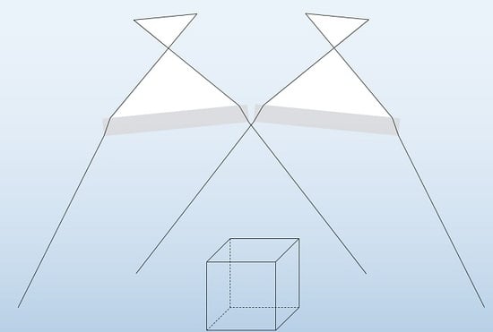
The dataset HS consists of a synthetic bundle in the form of a half-sphere (HS). The 2D object is made up of regularly spaced points at a distance of 250 mm. The 10 × 10 points result in a calibration fixture of 2500 mm × 2500 mm. The 36 camera positions reach down to 45° observation angle to simulate a realistic configuration (Figure 5). The average acquisition distance is 3.5 m as in dataset Cube. This dataset is created to simulate a different calibration fixture. In practice, often flat test-fields are used to calibrate stereo systems, as in [37]. The best configuration for a flat object is a half-sphere-shaped bundle. In real tasks, acquisition angles of less than 45° with respect to the targets on the calibration fixture often are avoided, since targets might not be measurable anymore, respectively have large elliptical eccentricity. Computer vision approaches often use such flat test-fields in the form of chessboard targets [37,38]. According to [29], 2D test-field calibrations result in less accurate and less robust parameter estimation. Furthermore, correlations between calibrated parameters usually are higher.
3.4. Variation of Convergence
The determinability of the relative orientation depends on the stereo configuration (Figure 6). Because of correlations between interior and exterior orientation parameters, the angle of convergence is critical when calibrating stereo systems in multimedia photogrammetry. To analyse the calibration results and their effect in object space in different setups, the convergence is varied for both datasets Cube and HS. Six different angles of convergence are simulated in 5° steps from 0° (parallel configuration) to 25° leading to the datasets shown in Table 1.
3.5. Variation of Air/Water Ratio
The refractive effects on photogrammetric calibration depend, apart from the refractive indices, on the distances the ray of light travels through each medium. In many applications a camera is mounted in a watertight housing, thus the interface is placed nearly perpendicularly right in front of the camera lens. In close-range applications, the ratio of distance through air and water can become close to 1/1 whereas in typical ROV applications the ratio becomes smaller (e.g., 1/300).
The datasets Cube and HS are varied at the air/water ratio to analyse the effects on the orientation parameters and the effects in object space. In particular, this means that the synthetic interface is moved along the optical axis towards the object space from a planar interface just in front of the lens to 50% of the acquisition distance. Overall, six ratios are simulated leading to six datasets for the cubic arrangement and further six for the spherical configuration (Figure 7, Table 2), by shifting the interface away from the cameras by 10% successively. The percentage of data do not take the glass interface into account, thus showing the ratio of the length of the path of light through air and water. The first datasets are simulated as a single medium case; therefore, no interface is present. The datasets in the second row represent the case of a typical underwater housing with an air/water depth ratio of 1/99 as used in ROV applications, whereas the latter datasets are valid only for ultra-close-range applications where the camera is very close to an object or in cases in which the object is close to an interface not mounted to the camera, as an aquarium glass pane. In this work, the acquisition distances are not varied; thus no real ultra-close-range application is simulated, but discrepancies in the mathematical model are transmissible. The relative relations between air/water are identical.
3.6. Quality Evaluation in Object Space via Forward Intersection
To evaluate the actual error in object space, 3D coordinates are calculated using the calibrated parameters of the relative and interior orientation. Besides the calibrated parameters, the error-free simulated image coordinates are used to perform the forward intersection. Thus, a process is simulated as a standard software would do. Refractive effects are modelled implicitly within the bundle adjustment of the calibration. Thus, a standard forward intersection can be calculated, not modelling the refractive interfaces. If the parameters model the setup properly, no significant error should occur in object space when intersecting error-free image coordinates of a stereo pair.
A test object of 500 mm × 500 mm is created and moved through the object space (Figure 8). The simulated 3D coordinates of this (moved) object can then be compared with the forward intersection results of one pair of images of the bundle. The object is shifted along the optical axis of the left camera in discrete steps of 100 mm, from just in front of the camera (once all five points are projected into both images) up to 6 m. Thus, approximately 50 test objects with five points each can be calculated via forward intersection and checked against nominal 3D coordinates for one image pair of the bundle. It would be possible to calculate each of the 36 stereo pairs. In the interest of clarity, one exemplary pair is analysed in this work. In the following, all analyses refer to this image pair of the specific bundle if not indicated otherwise.
4. Analysis of Calibration and Orientation for Planar Interfaces in Implicit Form
In this section, the analyses of the interior, exterior and relative orientation parameters for single and stereo camera systems, based on the synthetic data are presented. Furthermore, the effect of implicit modelling is analysed in object space to assess options and limits of implicit modelling with respect to the configuration of the system, including the shape of the calibration fixture. Besides the calibrated parameters, statistics and correlations of the conducted bundle adjustment are analysed. The goal of this analysis is to assess model discrepancy with respect to different setups. The configurations simulated underlie varying conditions and represent a variety of applications.
4.1. Single-Camera Bundle Adjustment
To analyse the exterior and interior orientations within a bundle adjustment, two datasets based on the setup of Figure 4 and Figure 5 are simulated for each dataset, Cube and HS. In Table 3, principal distance and radial-symmetric parameters of resulting datasets are listed. Furthermore, the introduced nominal values are listed in dataset 1.
For the datasets 2 and 3 (1SM-1/99), image coordinates without any refractive effects are used for the bundle adjustment, whereas the datasets 3 and 4 (1MM-1/99) contain error-free refracted image coordinates. The interface is simulated 20mm in front of the lens, thus leading to an air/water depth ratio of approximately 1/99. The bundle adjustment was performed using standard software not introducing any interfaces as parameters, and using the standard collinearity equations with the distortion model according to [15]. The interior and exterior orientations are determined within the bundle adjustment employing the object points as fixed reference points. Table 3 shows that the principal distance is longer in the multimedia case by a factor of 1.42 compared to the nominal value. Furthermore, the values of the radial distortion parameters increase significantly. According to [39], the principal distance c increases underwater by a factor equivalent to the refraction index of water. The authors of [40] present ratios of 1.335 to 1.345 in experimental setups within identical environmental conditions and show that the principal distance as well as the exterior orientations of a stereo camera system exhibit high discrepancies between in-air and in-water calibration. In [41], it is suggested not to overcome the refraction effects by camera calibration and shown how the principal distance behaves in calibration depending on the ratio of air and water within the path of light.
In underwater imaging, a pincushion radial symmetric distortion is typically introduced, since the path of light travels from air into a medium of higher refractive index. Thus, radial distortion parameters A become unequal to zero, when an underwater case is simulated. In contrast to the analysis of real datasets, analysing synthetic data allows for the comparison of the exterior orientations among different datasets.
Figure 9 shows the systematic shifts of exterior orientations between single-medium and multimedia bundles along the optical axes of the respective camera. For dataset Cube, these shifts of the camera position are 6.8 mm while for HS, they are 6.6 mm in size.
Due to high correlations, mainly between c and the EO translation parameter in the direction of the optical axis, it might occur that the principal distance, and the exterior orientation is calculated incorrectly. However, if calibrated parameters are used within one process such as bundle adjustment with self-calibration, these values represent the optimal mathematical solution, and systematical shifts of exterior orientations might be irrelevant. Present correlation between the principal distance and the translation parameter in the direction of the optical axis is similar for both datasets, Cube and HS, at a level of 0.75 in single media datasets as well as in the multimedia datasets. By reason of the flat calibration fixture, higher correlations are expected to appear. Probably, because of such optimal bundle configuration as in HS, correlations are not notably higher than in Cube, even though a flat calibration fixture is used.
When parameters are used in separate measurement tasks as when pre-calibration is conducted, the correlations might lead to incorrect results in object space. The fact that the calibration in the multimedia case can introduce an error to the interior (mainly the principal distance) and exterior orientation might become more relevant when the scale is provided not by reference points but by a stereo base only.
4.2. Stereo Camera Bundle Adjustment
The analysis of stereo camera calibration is conducted for the Cube and HS dataset variations. Two groups of simulated datasets are established. As presented in Section 3, the first group consists of datasets where the angle of convergence is varied. The second group consists of datasets, with translated interfaces, thus leading to varying air/water ratios.
The simulation of image coordinates for 36 image pairs is performed the same way as explained previously with the interface 20 mm in front of the principal point and a base of 200 mm. When no convergence is introduced, the following datasets can be generated as a stereo dataset:
- 2SM-0°-1/99
- 2MM-0°-1/99
When analysing these datasets, the same effects as in Section 4.1 can be observed. The principal distance becomes longer, and the radial distortion parameters differ significantly from the nominal parameters in multimedia case. In addition, the exterior orientations of the multimedia dataset show systematic translations in the direction of the optical axes as in the single-camera case illustrated in Figure 9. When the scale is provided by the relative orientation, it is essential that the relevant parameters are adjusted correctly. The following section discusses the behaviour of the relative orientation when using standard software and points out the critical aspect when the scale is provided by the relative orientation only. In the following subsections, relative and interior orientations are analysed and correlations depicted. Resulting errors in object space are quantified.
4.2.1. Variation of Convergence
The determinability of the relative orientation depends on the stereo configuration. The results in Table 4 show different datasets, whereat the angle of convergence varies by 5° at each dataset from 0° to 25°. First, only datasets of an air/water ratio of 1/99 are analysed.
The dataset 1 confirms that the mathematical model is correct for the single-medium case, since all parameters of the relative orientation equal the nominal parameters. As already noted, the camera positions of all multimedia datasets are systematically estimated further away from the object. Dataset 2 shows slightly different results for X0 (direction of stereo base) and Z0 (direction of the optical axis) of the relative orientation and the expected longer principal distance. This parallel dataset suggests a nearly correct estimation of the relative orientation, thus leading to the assumption that no significant scaling error is introduced. The convergent datasets show a significant change in relative orientation, whereby the most convergent configuration leads to the most affected orientation parameters. The convergent data of HS contain similar results, as Table 5 shows.
The parameters of the calibrated interior orientations remain nearly constant between different datasets. Also, the computed standard deviation of these parameters is not of noteworthy difference between the setups.
When analysing the correlations of the data, both datasets HS and Cube show similar trends. In general, the level of correlations is a little higher in the HS data. Some major correlations (higher than |0.5|) between relative and interior orientation can be identified (Table 6), where B represent the parameters of tangential and radial-asymmetric distortion according to [15]. Figure 10 shows the trend for increasing convergence exemplarily for the correlations of the principal distance and the translation parameters of the relative orientation. Relations between other parameters behave similarly showing higher correlations at larger angles of convergence. When the image coordinate is perfect, as in real case measurements, especially underwater, these correlations would lead to errors in correlated parameters. As Figure 10 implies, for parallel configurations (0°), discrepancies would rather occur in Z and/or c, while for convergent configurations (25°) discrepancies could also be highly possible in the direction of X, since the correlation of X and c converge to the one between Z and c with an increasing angle of convergence.
When analysing the correlations of one specific image of the bundle with the optical axis parallel to one of the coordinate system, large dependencies can be observed between the principal distance and the translation in the direction of the camera’s optical axis. Thus, calibration results might cause errors in the scale when the relative orientation is calculated incorrectly, and the exterior orientation is shifted. Besides the wrong scale, the absolute position of the determined coordinates might be incorrect. Scale can be corrected using scale bars as in [25] and validated using independent reference lines as in [20]. Regarding the absolute position of object points obtained from a stereo camera system, a quality assessment is difficult in praxis. Even though the absolute positioning is negligible for many applications, it might cause discrepancies when points in different absolute positions, underlying different positioning errors, are used to determine relevant measurements (e.g., fish length).
As described in Section 3.6, the effect of calibrated parameters is quantified in object space. Figure 11 visualises the 3D deviations from reference points (centre point of the moved reference object, Figure 8) to the calculated coordinates from forward intersection using one image pair and calibrated interior and relative orientation parameters.
Deviations are higher for larger angles of convergence and form a steeper ‘v’ around the calibration distance. It can be seen that the lowest deviation is not exactly at the calibration distance and is different for the different datasets. All images of the bundle, having different acquisition distances and image coordinates, are part of the network; therefore, the calibrated parameters fit the whole bundle optimal. Probably, because only a single image pair is used to determine spatial intersection, the deviation is not the lowest at exact calibration distance. As for the 25° dataset, the lowest deviations of intersected points are present at ~4000 mm, thus the minimum of deviations is ~500 mm further than the average calibration distance.
Due to imperfect calibration all over the image sensor, image coordinates at the image borders, which occur more often in convergent setups, result in less accurate object coordinates, despite error-free image coordinates being used for calibration and forward intersection. According to [42,43], the physical model of refraction fits much worse at the image borders than in the image centre. Thus, even with only error-free image coordinates being present, the calibration can be assumed to be of decreasing quality towards the image borders. The visualised deviations only depend on the calibrated interior and relative orientation parameters. The quality of spatially intersected points highly depends of the position of the image sensor and related calibrated parameters. Since the calibration is conducted using several images, with their points covering different sensor areas, a single forward intersection might not be best at the average calibration distance (see dataset 25° in Figure 11).
Besides an absolute translation deviation along the observation axis of the particular image pair, a deviation in the scale can be observed in spatially intersected points. The implicit calibration, thus leads to two main effects—first, an absolute translation in the object space, second a scale error. The error in scale can be quantified by performing a 3D similarity transformation of five spatially intersected points at one step (see Figure 8) to the five reference object points. The determined scale parameter is visualised in Figure 12. It can be observed that the scale becomes larger when the reference object is moved away from the camera, especially for more converged configurations. Due to the changing positions on the image sensor, the intersected points underlie different conditions. Also, when moving the object very close towards the camera, a quick change of scale can be observed. While the absolute positioning error remains stable in the range between 1 m and 2 m, the scale is majorly affected. Even for the parallel setup (0°), an error in scale would be introduced when the acquisition distance is low.
The analyses of the dataset HS show similar results to presented data of Cube. No mentionable systematic differences exist.
4.2.2. Variation of Air/Water Ratio
Besides the convergence, the air/water ratio is varied as described in Section 3.5. Table 7 shows the calibrated parameters of the relative orientation and the principal distance.
The dataset 2 represents the case of a typical underwater housing with an air/water depth ratio of 1/99. This dataset shows only a small difference in the stereo base. When moving the interface away from the camera, the error of the relative orientation raises up to more than 2 mm in translation and 0.03° in rotation (2MM-0°-50/50). The results are not stable, not even with synthetic data. They highly depend on the configuration of the bundle and the correlations between critical parameters. As expected, the principal distance becomes smaller when the percentage of water is decreased. As presented by [41], using standard software might lead to contrasting results regarding the principal distance. Compared with the results of convergent datasets (Section 4.2.1), the principal distance is calibrated significantly different. Furthermore, in contrast to the experiments of the previous section, the variation of the interface leads to large errors of the relative orientation in Z0, which represents the direction of the optical axis of the stereo camera (Table 8).
The principal distance of dataset HS is calibrated up to 0.6 mm shorter by moving the interface towards a ratio of 50/50. Also, the variation in X0 is higher than in Cube datasets. Generally, the trend of calibrated parameters of the relative orientation is confirmed and similar to one of the Cube datasets.
Presented correlations of datasets of different air/water ratios are slightly lower than for convergent datasets. The major correlations are listed in Table 9. Fewer parameters correlate by more than 0.5 compared to convergent setups. Figure 13 shows exemplarily the trend of correlations of the principal distance and the translation parameter of the relative orientation. In contrast to the correlations of convergent datasets (Figure 9), the correlations behave stable between different datasets. When the interface is moved towards to calibration fixture, no relevant change of correlations arises.
Again, to quantify the discrepancies of the implicit system calibration, deviations in object space are calculated. Figure 14 visualises the 3D deviations from the reference points (centre point of the moved reference, according to Figure 8) to the calculated coordinates of the Cube datasets. The results are based on the same image pairs as for the convergent dataset analyses. It can be seen that the 50/50 dataset creates the largest deviations. The dataset with the interface just in front of the lens (1/99) has almost no error in forward intersection, thus can be modelled well by the implicit calibration. The deviations rise up to more than 40 mm when the intersection is performed very close to the camera. Compared to the deviations of the convergence dataset (Figure 11), the deviations of the ratio datasets are not only much higher but also form a steeper ‘v’ around the calibration distance, which means that deviations in the object space will occur when the acquisition distance is significantly shorter or longer than the calibration distance.
It is mentionable that the HS dataset again proves the trends but has higher deviations for object points further away from the camera (larger slope). For closer simulated acquisition distances, the plane 2D calibration fixture leads to lower deviations in the object space (Figure 15).
As for convergent data, a 3D transformation of the intersected object (five points, according to Figure 8) to the reference is performed. The resulting scale parameters are visualised for each dataset in Figure 16. The geometry of the five-point pattern is scaled in object space by a factor of up to 0.999 at 6 m acquisition distance. When the acquisition distance becomes very short, the error in scale is increased promptly. In contrast to the data of Cube, the data of HS show a larger scale factor (up to 1.002 at 6 m for 2MM-0-50/50) and have the largest scale in the dataset 50/50. At the range of ±2.5 m of the calibration distance, the 50/50 ratio shows the highest scale error.
4.3. Assessment of Simulated Data
Deviations in object space increase with longer distances. In practical applications, this effect is well known and due to poor intersection angles at far points. In underwater cases, the turbidity of large water columns usually decreases the quality of further points, in addition, the simulated data neither underlie any degradation effects nor is it affected by any target image measurement quality. Thus, the angle of intersection is irrelevant for the accuracy of intersected points in this study. However, the simulated data still shows the tendency to result in worse intersection at larger acquisition distances.
Since no errors are present in synthetic data, only the effect of the implicit modelling is responsible for remaining deviations. The only influences on the intersected points are the calibrated parameters of the relative and interior orientations. Depending on their quality and mathematical validity, the intersection quality is determined. Convergent configurations show worse results than parallel. As a result of the convergent setup, the simulated image coordinates are further towards the image borders in convergent datasets. The calibrated parameters of both interior orientation and relative orientation seem to fit less towards the image borders. In practical applications, the image border should be excluded as much as possible since other degradation effects intensify poor calibration results at the image borders.
As for an increased angle of convergence, the higher ratios show a steeper ‘v’ in deviations in object space. In general, varying ratios result in higher deviation in object space. Errors also increase with distances which is consistent with the findings of [9]. When the interface is moved towards the object, the mathematical model does not fit as well as it does when the interface is just in front of the camera. Due to present refractions, the assumption of a single projection centre is invalid [42,43]. These discrepancies from the real physical model are increased when the air/water ratio is increased. This is particularly crucial when the interface is not mounted directly in front of the lens or when the water column is not very large. Thus, especially in close-range applications with short acquisition distances, the invalidity of the assumption of one projection centre needs to be taken into account.
Due to correlations of exterior and interior parameters, besides the geometrical deviation expressed mainly as scaling errors, the absolute position of intersected points might be incorrect. The exterior orientations can barely be validated in real applications. However, the simulated data allows for validation. As shown in Figure 9, the exterior orientation is shifted in bundle adjustment. The deviations of intersected points in object space have their major component in the direction of the optical axis. It might be irrelevant for many applications that the object points are shifted, but when object points of different acquisition distance are combined for final results (e.g., fish length of a fish pointing towards the camera), the effect of wrong absolute positioning also affects the geometrical quality. Validating stereo reconstructions just by using scale bars in object space is crucial regarding the absolute position. It is recommended when scale bars are used for validation, that these point towards the camera in order to quantify the deviations of different acquisition distances.
The deviations of a combination of 5° convergence at a ratio of 10/90 is exemplary shown in Figure 17. It can be seen that the implicit modelling leads to errors of <2 mm in a range of 2 m (2–4 m). The acquisition distances far from the calibration distance would lead to large errors. Low ratios at a preferably parallel setup result in the lowest deviations, according to the modelling discrepancies of implicit modelling.
5. Analysis of Calibration and Orientation for Planar Interfaces in Explicit Form
As stated in the previous section, the implicit modelling of refractive interfaces is critical due to highly correlated parameters. In this section, the synthetic data from Section 3 will be analysed using a strict explicit model. It is assumed that due to the strict model, the synthetic data will not lead to systematic errors in object space as observed when running standard software using implicit modelling. The presented explicit analyses are also conducted for real data experiments in Section 6.
5.1. Explicit Modelling
The use of standard software and the implicit modelling of refractive effects can lead to relevant errors in the object space. Therefore, a multimedia bundle adjustment explicitly modelling the refractive interfaces according to [19] is implemented. In real tasks, the interior orientation could be determined by a standard calibration procedure in the air using existing software products and toolboxes. If mechanically possible, the relative orientation could also be calibrated in the air (see case 4 and 5, Figure 1). The simultaneous determination of the parameters of interfaces, interior and, relative orientation (see case 3, Figure 1) is theoretically possible, but will probably lead to a very unstable numerical system.
To be able to calculate a relative orientation in the multimedia case, the following parameters are introduced to the bundle adjustment:
| nair | = refractive index of air |
| nglass | = refractive index of glass |
| nwater | = refractive index of water |
| N1x, N1y, N1z, d | = plane parameters of interface 1 |
| N2x, N2y, N2z, d2 | = plane parameters of interface 2 |
| X0, Y0, Z0 | = translation of the relative orientation |
| ω, φ, κ | = rotation of relative orientation |
The first interface represents the plane of refraction from medium air to glass, the second one the plane of refraction from glass to water. The thickness of the interfaces, as well as the refractive indices of air and glass, are assumed to be known, whereas the other added parameters are treated as unknowns.
5.2. Synthetic Data
First of all, synthetic datasets are analysed again using the multimedia bundle adjusting the exterior orientations and the relative orientation. The results of the adjustment equal the nominal synthetic values. Furthermore, a combination of the most critical datasets (25° convergence and air/water ratio of 50/50) is adjusted via the multimedia bundle. Even this critical configuration converges correctly (Table 10), thus proving the implementation of the multimedia bundle adjustment.
Initial values for unknowns can be received by standard software ignoring the refractive physics processing bundle adjustment. Due to highly correlated parameters and possible poor bundle configurations, the implementation needs to be robust in order to deal with bad initial values. To prove the robustness of the process, realistic noise for observations, as well as for the first approximations for the unknown values, is introduced as follows:
| nwater | ± 0.01 |
| Image coordinates | ± 1 pixel |
| Translation of exterior orientations | ± 200 mm |
| Rotation of exterior orientations | ± 1° |
The results converge to the same values as those without noise, which verifies our implementation with respect to the modelled parameters. Furthermore, the results of spatially intersected points do not show any significant errors in the object space, as expected with simulated data.
6. Experiments
To prove the findings of the analyses of the synthetic data and to quantify the real deviations, the following experiment is conducted. Two stereo camera setups are realised in the laboratory using both a 2D and a 3D calibration fixture. Monochromatic cameras with a sensor of 2048 × 2048 pixel (5.5 µm pixel pitch) are used in this study. After a description of the experiments, quantifying analyses lead to an assessment of the results.
6.1. Description of the Experiments
In Figure 18, the setups of the experiments can be seen. Two setups are realised—one parallel and one convergent setup at an angle of convergence of ~27°. Furthermore, an exemplary image in the air (Figure 18c, top) and through water (Figure 18c, bottom) are presented. The inverted radial distortion, introduced by refractive effects, can be noted at the image border. In both cases, 2D and 3D calibration fixtures are used to calibrate the stereo camera, thus yielding four datasets. Both objects consist of 246 uniformly distributed points of 1 mm in diameter, whereat the points are arranged in two levels (20 mm in height) at the 3D object and in only one at the 2D (flat) object. Twelve image pairs are taken for each calibration in a similar acquisition arrangement rotating and tilting the calibration fixture leading to an overall redundancy of 7000–10,000 depending on the setup. The average acquisition distance is 180 mm for all experiments.
6.2. Calibration Parameters
First, the interior orientation of each camera is calibrated in air using bundle adjustment. The points on the calibration fixtures are introduced as unknown tie points; thus the position of the targets is derived as part of the self-calibration. Introduced predefined distances between some points define the scale within the network. The calibrated parameters of the interior orientation are listed in Table 11 exemplary for the parallel dataset with the 3D calibration fixture used. Typical pincushion distortion (A-Parameters) and an increased principal distance are calibrated in the underwater case. The resulting radial distortion is visualised in Figure 19. It can be seen that the curve of the radial distortion gets steeper towards the image edges in underwater implicit modelling. Furthermore, the distortion underwater is of an opposite algebraic sign compared to the distortion of the calibration in air.
Due to the instability of the underwater camera housings, the relative orientation in air and underwater would not be comparable. However, in the case of the parallel setup, the cameras are placed in front of an aquarium; thus the relative orientation of the multimedia setup can be compared to the parameters determined in air. Table 12 shows relative orientation parameters for the four multimedia setups and the parallel configuration in air. Besides the four implicit calibrations (No. 1,2,5,6), the images of the bundles are used to conduct an explicit calibration as described in Section 5.1, introducing the interior orientation of the calibration in air as fixed parameters. Thus, in both analyses (implicit and explicit), the same imagery is used.
It can be seen that the calibrated parameters differ significantly in most cases. While the differences between different calibration fixtures are rather small (compare dataset 1 and 2, also 5 and 6) but still significant, the explicit calibration determine the relative orientation parameters completely different. To quantify an error in the object space, it is inevitable to calculate 3D points. Since different adjusted interior and exterior orientations form a mathematical model with the adjusted relative orientation, the whole system needs to be analysed. As done for synthetic data, forward intersection is used to compute 3D points from one image pair based on the adjusted orientations.
6.3. Deviations in Object Space
In order to quantify deviations in the object space, the 2D calibration fixture is shifted through the object space after calibration and acts as an independent test object. Nine separate image pairs are acquired in different distances from the fixed stereo camera (position 1–9). Independent forward intersections can be calculated using the image coordinates of these nine image pairs. Based on the same image coordinates, four different relative and interior orientations can be introduced to the forward intersection to calculate 3D points. Thus, all calibrated parameters of parallel experiments can be used and compared against each other as well as the four convergent data. As it turns out, some positions are too far out of focus and cannot be analysed. Due to the limited DOF of ~25 mm, the range in the object space of the shifted 2D test object is also limited. Since slightly blurred images can also be analysed, the range in the object space, where image coordinates can still be measured with standard software is approximately 100 mm. Figure 20 and Figure 21 show the 3D deviations of the independent spatially intersected object points to the reference. The points from intersection need to be transformed to be able to compare geometries; thus no absolute position in the object space can be evaluated yet. Between every position, the test object is moved ~25 mm towards the cameras, from 250 mm at position 5 to 150 mm at position 1. Positions 3 and 4 are close to the calibration distance of 180 mm on average.
First, the parallel setup (Figure 20) is analysed. As expected, the mean deviation is the smallest near the calibration distance. The explicit method is much better (approx. factor 2) at further positions and similar in quality near the calibration distance. The implicit model seems to be “more valid” for a certain range near the calibration distance as simulations also identified. The performance of the spatial calibration fixture is slightly better than that of the 2D calibration fixture. Furthermore, the further away the object is, the worse the angle of intersection becomes and due to limited DOF, the quality of image measurement is also worse. Especially, the component in the direction of the optical axis is thus defective.
In case of the convergent experiment, the results do not appear as expected. In general, the 2D calibration fixture performs much better than the 3D object—our implementation of explicit modelling results in large errors underlying systematic spreading. Even when an explicit model is used, high correlations might be present in the bundle adjustment, and furthermore, pinhole model is still adopted after refracting the image ray. As [42] and [43] discuss in detail, the pinhole model does not hold true underwater due to arising caustics. Existing errors might also relate to the fact that initial values for the explicit modelling are not provided well enough by the bundle adjustment of the standard software (implicit model). Further investigations must be performed in order to see the limits and restrictions of the explicit modelling regarding initial values and configurational setups.
As observed for implicit modelling, the initial values for the implicit form are also important. The software used for this work calculates slightly different interior orientation parameters but significantly different exterior orientation parameters according to the initial values for the interior orientation within the bundle adjustment. It is recommended multiplying the (in air) known focal length by a factor of ~1.4 in order to introduce reasonable initial values for an implicit bundle adjustment when standard software is used.
Besides the geometrical evaluation, a relative comparison of absolute positioning in the object space can be performed. Figure 22 shows the mean difference of the intersected points underlying the calibration parameters of 2D calibration to the points intersected underlying parameters of 3D calibration. No absolute positioning reference is known in the experiments; therefore, no statement can be given as to which calibration parameters result in more accurate results. However, a significant difference in the object space can be determined. Despite the identical geometry of both sets, 2D and 3D calibration have mean deviations between 0.55 mm and 0.1 mm (Figure 20), whereas the absolute difference is much higher in parallel cases and a little higher in convergent cases. When calculating the differences, it is visible that the difference is clearly in the direction of the optical axis of the cameras as can be found in Figure 23 exemplary.
7. Conclusions
This contribution refers to different articles of underwater photogrammetry and computer vision. An overview of system configurations and calibration techniques is given, and the investigation of the behaviour of relative and interior orientation of stereo camera systems with planar interfaces within the bundle adjustment is covered. Synthetic datasets prove theoretical considerations and show how implicit calibration affects the 3D reconstruction. It can be seen that the error in the object space highly depends on the setup of the cameras and interfaces. Furthermore, the configuration of the bundle and of the reference object for calibration affect the dimension of the introduced errors. The correlations between the principal distance and the camera positions become critical when the scale is provided by the relative orientation of multi-camera systems. As already reported in [9,44], systematic errors remain due to the invalid assumption of a single projection centre. Due to error-free simulations and analyses of correlations, these errors can be classified in absolute location deviations and geometric deformations. In the real datasets only a relative comparison of absolute positioning is possible. It can be seen that the implicit calibration using a spatial calibration fixture leads to the best (implicit) results in the parallel setup. In convergent setup, the 2D calibration results in better intersection points. All datasets show the trend to produce poor results when the acquisition distance differs from the one of the calibration. The explicit modelling showed the best results in parallel setup. In explicit modelling, the 3D calibration fixture also leads to better results. The explicit modelling is able to increase accuracy by a factor of 1.1–2 depending on the acquisition distance. However, remaining systematic deviations are still present in the forward intersected points. The convergent datasets do not show any improvement of results when calibration is conducted in explicit form. This might be due restrictions of the explicit implementation regarding initial values or due to modelling discrepancies according to [43].
In real tasks, many influences, such as the turbidity of the water, affect the final measurement. In general, it seems to be difficult to separate those influences and the resulting deviations (geometrical and positioning errors) in real datasets. In multimedia photogrammetry, a loss of accuracy is expectable. Depending on the configuration of a multi-camera system and on the needs of the application, it might be reasonable to use implicit modelling for multimedia photogrammetry. Especially for parallel setups with the interface just in front of the lens, loss in accuracy due to implicit modelling might be acceptable in some applications. However, it is highly recommended not to neglect refractive interfaces in general.
Using a dome port is probably a suitable solution for many applications since standard software can be used. As stated by [21], small misalignments of a dome port do not produce departures from the geometrical model in standard photogrammetry. However, besides the fact that an imperfectly arranged dome port can introduce systematic errors and establishing a pre-defined focusing distance is not trivial when using dome ports [21], there are good reasons to use flat ports (costs, installation size, easier to mount).
Regardless of the port and calibration strategy, independent validation should be conducted on site, using reference objects when accuracy is a crucial aspect of the desired application. If possible, reference objects with known absolute position could help to quantify the error budget according to the absolute positioning in stereo multimedia cases.
Author Contributions
Conceptualisation, O.K.; Methodology, O.K., Data simulation, O.K. and R.R.; Software, R.R. and O.K., Investigations, O.K.; visualisation, O.K.; Writing–original draft, O.K.; Writing–review and editing, R.R. and T.L. All authors have read and agreed to the published version of the manuscript.
Funding
This research was funded by the European Regional Development Fund (EFRE, ZW 6-85003503 and ZW 6-85007826) and by the Volkswagen Foundation, Germany (ZN3253).
Conflicts of Interest
The authors declare no conflict of interest.
References
- kbvresearch.com. Underwater Camera Market Size. Available online: https://www.kbvresearch.com/underwater-camera-market-size/ (accessed on 28 November 2019).
- Datainsightspartner.com. Underwater Drones Market Size Estimation, in-Depth Insights, Historical Data, Price Trend, Competitive Market Share & Forecast 2019–2027. Available online: https://datainsightspartner.com/report/underwater-drones-market/61 (accessed on 28 November 2019).
- Shortis, M.; Ravanbakskh, M.; Shaifat, F.; Harvey, E.S.; Mian, A.; Seager, J.W.; Culverhouse, P.F.; Cline, D.E.; Edgington, D.R. A review of techniques for the identification and measurement of fish in underwater stereo-video image sequences. In SPIE Optical Metrology; Remondino, F., Shortis, M.R., Beyerer, J., Puente León, F., Eds.; SPIE: Munich, Germany, 2013. [Google Scholar]
- Torisawa, S.; Kadota, M.; Komeyama, K.; Suzuki, K.; Takagi, T. A digital stereo-video camera system for three-dimensional monitoring of free-swimming Pacific bluefin tuna, Thunnus orientalis, cultured in a net cage. Aquat. Living Resour. 2011, 24, 107–112. [Google Scholar] [CrossRef] [Green Version]
- Menna, F.; Nocerino, E.; Nawaf, M.M.; Seinturier, J.; Torresani, A.; Drap, P.; Remondino, F.; Chemisky, B. Towards real-time underwater photogrammetry for subsea metrology applications. In OCEANS 2019; IEEE: Marseille, France, 2019; pp. 1–10. [Google Scholar]
- Bruno, F.; Lagudi, A.; Collina, M.; Medaglia, S.; Davidde Petriaggi, B.; Petriaggi, R.; Ricci, S.; Sacco Perasso, C. Documentation and monitoring of underwater archaeological sites using 3d imaging techniques: The case study of the “nymphaeum of punta epitaffio” (baiae, naples). Int. Arch. Photogramm. Remote Sens. Spat. Inf. Sci. 2019, XLII-2/W10, 53–59. [Google Scholar] [CrossRef] [Green Version]
- Costa, E. The progress of survey techniques in underwater sites: The case study of cape stoba shipwreck. Int. Arch. Photogramm. Remote Sens. Spat. Inf. Sci. 2019, XLII-2/W10, 69–75. [Google Scholar] [CrossRef] [Green Version]
- Kahmen, O.; Rofallski, R.; Conen, N.; Luhmann, T. On scale definition within calibration of multi-camera systems in multimedia photogrammetry. Int. Arch. Photogramm. Remote Sens. Spat. Inf. Sci. 2019, XLII-2/W10, 93–100. [Google Scholar] [CrossRef] [Green Version]
- Shortis, M. Calibration Techniques for Accurate Measurements by Underwater Camera Systems. Sensors (Basel) 2015, 15, 30810–30826. [Google Scholar] [CrossRef] [Green Version]
- Boutros, N.; Shortis, M.R.; Harvey, E.S. A comparison of calibration methods and system configurations of underwater stereo-video systems for applications in marine ecology. Limnol. Oceanogr. Methods 2015, 13, 224–236. [Google Scholar] [CrossRef]
- Massot-Campos, M.; Oliver-Codina, G. Optical Sensors and Methods for Underwater 3D Reconstruction. Sensors (Basel) 2015, 15, 31525–31557. [Google Scholar] [CrossRef] [PubMed] [Green Version]
- Höhle, J. Zur Theorie und Praxis der Unterwasser-Photogrammetrie; Deutsche Geodätische Kommission: München, Germany, 1971. [Google Scholar]
- Maas, H.-G. Digitale Photogrammetrie in der Dreidimensionalen Strömungsmesstechnik. Ph.D. Thesis, ETH Zürich—Dissertation Nr. 9665, Zürich, Switzerland, 1992. [Google Scholar]
- Mandlburger, G. A case study on through-water dense image matching. Int. Arch. Photogramm. Remote Sens. Spat. Inf. Sci. 2018, XLII-2, 659–666. [Google Scholar] [CrossRef] [Green Version]
- Brown, D.C. Close-Range Camera Calibration. Photogramm. Eng. 1971, 37, 855–866. [Google Scholar]
- Kotowski, R. Zur Berücksichtigung Lichtbrechender Flächen im Strahlenbündel; Zugl.: Bonn, Univ., Diss., 1986; Beck: München, Germany, 1987; ISBN 3769693795. [Google Scholar]
- Bräuer-Burchardt, C.; Heinze, M.; Schmidt, I.; Kühmstedt, P.; Notni, G. Compact handheld fringe projection based underwater 3d-scanner. Int. Arch. Photogramm. Remote Sens. Spat. Inf. Sci. 2015, XL-5/W5, 33–39. [Google Scholar] [CrossRef] [Green Version]
- Maas, H.-G. A modular geometric model for underwater photogrammetry. Int. Arch. Photogramm. Remote Sens. Spat. Inf. Sci. 2015, XL-5/W5, 139–141. [Google Scholar] [CrossRef] [Green Version]
- Mulsow, C. A flexible multi-media bundle approach. Int. Arch. Photogramm. Remote Sens. Spat. Inf. Sci. 2010, XXXVIII/5, 472–477. [Google Scholar]
- Menna, F.; Nocerino, E.; Remondino, F. Flat versus hemispherical dome ports in underwater photogrammetry. Int. Arch. Photogramm. Remote Sens. Spat. Inf. Sci. 2017, XLII-2/W3, 481–487. [Google Scholar] [CrossRef] [Green Version]
- Nocerino, E.; Menna, F.; Fassi, F.; Remondino, F. Underwater calibration of dome port pressure housings. Int. Arch. Photogramm. Remote Sens. Spat. Inf. Sci. 2016, XL-3/W4, 127–134. [Google Scholar] [CrossRef] [Green Version]
- Menna, F.; Nocerino, E.; Fassi, F.; Remondino, F. Geometric and Optic Characterization of a Hemispherical Dome Port for Underwater Photogrammetry. Sensors (Basel) 2016, 16, 48. [Google Scholar] [CrossRef] [Green Version]
- Menna, F.; Nocerino, E.; Remondino, F. Optical aberrations in underwater photogrammetry with flat and hemispherical dome ports. In Videometrics, Range Imaging, and Applications XIV; SPIE: Munich, Germany, 2017; pp. 26–27. [Google Scholar]
- Shortis, M.; Harvey, E.; Seager, J. A Review of the Status and Trends in Underwater Videometric Measurement. In Proceedings of the SPIE Conference 6491, Videometrics IX, IS&T/SPIE Electronic Imaging, San Jose, CA, USA, 28 January–1 February 2007. Invited paper. [Google Scholar]
- Menna, F.; Nocerino, E.; Troisi, S.; Remondino, F. A photogrammetric approach to survey floating and semi-submerged objects. In SPIE Optical Metrology; Remondino, F., Shortis, M.R., Beyerer, J., Puente León, F., Eds.; SPIE: Munich, Germany, 2013; 87910H. [Google Scholar]
- Johnson-Roberson, M.; Pizarro, O.; Williams, S.B.; Mahon, I. Generation and visualization of large-scale three-dimensional reconstructions from underwater robotic surveys. J. Field Robotics 2010, 27, 21–51. [Google Scholar] [CrossRef]
- Rofallski, R.; Luhmann, T. Fusion von Sensoren mit optischer 3D-Messtechnik zur Positionierung von Unterwasserfahrzeugen. In Hydrographie 2018, Trend zu Unbemannten Messsystemen; Wißner-Verlag: Augsburg, Germany, 2018; pp. 223–234. ISBN 978-3-95786-165-8. [Google Scholar]
- Luhmann, T.; Fraser, C.; Maas, H.-G. Sensor modelling and camera calibration for close-range photogrammetry. ISPRS J. Photogramm. Remote Sens. 2016, 37–46. [Google Scholar] [CrossRef]
- Wester-Ebbinghaus, W. Verfahren zur Feldkalibrierung von photogrammetrischen Aufnahmekammern im Nahbereich. In Kammerkalibrierung in der Photogrammetrischen Praxis; Reihe, B., Kupfer, G., Wester-Ebbinghaus, W., Eds.; Heft Nr. 275; Deutsche Geodätische Kommission: München, Germany, 1985; pp. 106–114. [Google Scholar]
- Luhmann, T. Erweiterte Verfahren zur Geometrischen Kamerakalibrierung in der Nahbereichsphotogrammetrie; Beck: München, Germany, 2010; ISBN 978-3-7696-5057-0. [Google Scholar]
- Bruno, F.; Bianco, G.; Muzzupappa, M.; Barone, S.; Razionale, A.V. Experimentation of structured light and stereo vision for underwater 3D reconstruction. ISPRS J. Photogramm. Remote Sens. 2011, 66, 508–518. [Google Scholar] [CrossRef]
- Drap, P.; Seinturier, J.; Hijazi, B.; Merad, D.; Boi, J.-M.; Chemisky, B.; Seguin, E.; Long, L. The ROV 3D Project. J. Comput. Cult. Herit. 2015, 8, 1–24. [Google Scholar] [CrossRef]
- Luhmann, T.; Robson, S.; Kyle, S.; Boehm, J. Close-Range Photogrammetry and 3D Imaging, 3rd ed.; De Gruyter: Berlin, Germany; Boston, MA, USA, 2020; ISBN 9783110607246. [Google Scholar]
- Wester-Ebbinghaus, W. Einzelstandpunkt-Selbstkalibrierung. Ein Beitrag zur Feldkalibrierung von Aufnahmekammern; Zugl.: Bonn, Univ., Habil.-Schr., 1982; Beck: München, Germany, 1983; ISBN 3769693396. [Google Scholar]
- Ekkel, T.; Schmik, J.; Luhmann, T.; Hastedt, H. Precise laser-based optical 3d measurement of welding seams under water. Int. Arch. Photogramm. Remote Sens. Spat. Inf. Sci. 2015, XL-5/W5, 117–122. [Google Scholar] [CrossRef]
- VDI. VDI/VDE. 2634.1: Optical 3-D Measuring Systems—Imaging Systems with Point-by-Point Probing; VDI: Düsseldorf, Geramny, 2002. [Google Scholar]
- Costa, C.; Loy, A.; Cataudella, S.; Davis, D.; Scardi, M. Extracting fish size using dual underwater cameras. Aquac. Eng. 2006, 35, 218–227. [Google Scholar] [CrossRef]
- Buschinelli, P.D.V.; Matos, G.; Pinto, T.; Albertazzi, A. Underwater 3D shape measurement using inverse triangulation through two flat refractive surfaces. In OCEANS 2016 MTS/IEEE, Monterey, CA, USA, 19–23 September 2016; IEEE: Piscataway, NJ, USA, 2016; pp. 1–7. ISBN 978-1-5090-1537-5. [Google Scholar]
- Lavest, J.M.; Rives, G.; Laprest, J.T. Dry camera calibration for underwater applications. Mach. Vis. Appl. 2003, 13, 245–253. [Google Scholar] [CrossRef]
- Rahman, T.; Anderson, J.; Winger, P.; Krouglicof, N. Calibration of an Underwater Stereoscopic Vision System. In 2013 OCEANS—San Diego; IEEE: San Diego, CA, USA, 2013; pp. 1–6. [Google Scholar] [CrossRef]
- Agrafiotis, P.; Georgopoulos, A. Camera constant in the case of two media photogrammetry. Int. Arch. Photogramm. Remote Sens. Spat. Inf. Sci. 2015, XL-5/W5, 1–6. [Google Scholar] [CrossRef] [Green Version]
- Sedlazeck, A.; Koch, R. Calibration of Housing Parameters for Underwater Stereo-Camera Rigs. In British Machine Vision Conference 2011; Hoey, J., McKenna, S., Trucco, E., Zhang, J., Eds.; BMVA Press: Dundee, UK, 2011; pp. 118.1–118.11. [Google Scholar]
- Sedlazeck, A.; Koch, R. Perspective and Non-perspective Camera Models in Underwater Imaging—Overview and Error Analysis. In Outdoor and Large-Scale Real-World Scene Analysis; Hutchison, D., Kanade, T., Kittler, J., Kleinberg, J.M., Mattern, F., Mitchell, J.C., Naor, M., Nierstrasz, O., Pandu Rangan, C., Steffen, B., et al., Eds.; Springer: Berlin/Heidelberg, Germany, 2012; pp. 212–242. ISBN 978-3-642-34090-1. [Google Scholar]
- Maas, H.-G. On the Accuracy Potential in Underwater/Multimedia Photogrammetry. Sensors (Basel) 2015, 15, 18140–18152. [Google Scholar] [CrossRef] [PubMed]
Figure 1.
System components, calibration approaches for underwater photogrammetric systems. The left side illustrates options of configuration for single-camera usage; the right side illustrates options for multi-camera systems. Approaches 1 can be declared as unreasonable strategies, approaches 2 are standard strategies using standard software, explicit modelling approaches 3 are not part of this work but theoretically possible, approaches 4 and 5 model refractive effects explicitly using a known IO.

Figure 2.
Schema of the creation of synthetic datasets. After error-free images, the coordinates are calculated via strict ray tracing, the calibration is conducted using standard software and implicit modelling. The 3D coordinates are calculated via forward intersection of a stereo image pair, based on the standard model. These coordinates are compared to the nominal values of simulated test object coordinates.

Figure 3.
Exemplarily configuration of the interfaces. A plane interface (10 mm in thickness) of isotropic glass is simulated 20 mm in front of the principal point.
Figure 3.
Exemplarily configuration of the interfaces. A plane interface (10 mm in thickness) of isotropic glass is simulated 20 mm in front of the principal point.

Figure 4.
Setup of the synthetic dataset Cube. Blue points (36) indicate the positions of the cameras, red points (100) indicate the cubic arranged object points (a). Cubic test object, according to VDI/VDE 2634.1 (b).
Figure 4.
Setup of the synthetic dataset Cube. Blue points (36) indicate the positions of the cameras, red points (100) indicate the cubic arranged object points (a). Cubic test object, according to VDI/VDE 2634.1 (b).

Figure 5.
Half-sphere-shaped bundle. Green dots indicate 10 × 10 points of the calibration fixture. The points are spaced at 250 mm in each direction. Simulated stereo cameras are rotated around the optical axis by 90° at each position. The basis is 200 mm.
Figure 5.
Half-sphere-shaped bundle. Green dots indicate 10 × 10 points of the calibration fixture. The points are spaced at 250 mm in each direction. Simulated stereo cameras are rotated around the optical axis by 90° at each position. The basis is 200 mm.

Figure 6.
Convergent stereo camera setup with bundle-invariant interfaces.

Figure 7.
Illustration of the refractive effects with different air to water ratio. The ratios vary from 1% air and 99% water (a) to a 50/50 configuration (b).
Figure 7.
Illustration of the refractive effects with different air to water ratio. The ratios vary from 1% air and 99% water (a) to a 50/50 configuration (b).

Figure 8.
Test object with five points moved 6 m in 100 mm steps along the optical axis of the left camera.
Figure 8.
Test object with five points moved 6 m in 100 mm steps along the optical axis of the left camera.

Figure 9.
Setup of the synthetic datasets. Blue points indicate the positions of the cameras, red points indicate the cubically arranged object points of dataset Cube (a) and object points of dataset HS (b), respectively. The arrows indicate the offset of the camera positions of dataset 2 and 4 and of 3 and 5 according to Table 3.

Figure 10.
Correlations between translation parameters of the relative orientation (X, Y, Z) and the principal distance c as a function of the convergence of the stereo configuration.
Figure 10.
Correlations between translation parameters of the relative orientation (X, Y, Z) and the principal distance c as a function of the convergence of the stereo configuration.

Figure 11.
3D deviations of the forward intersected points to the reference object points for 6 m through the object space. Different datasets of varying convergence of Cube and the average calibration distance are visualised.
Figure 11.
3D deviations of the forward intersected points to the reference object points for 6 m through the object space. Different datasets of varying convergence of Cube and the average calibration distance are visualised.

Figure 12.
Factors of the scale of a 3D similarity parameter transformation of each five-point object in object space to the corresponding reference five-point object. The scale is calculated for 6 m (each 100 mm) and visualised for the object space. Different datasets of varying convergence of Cube and the average calibration distance are visualised.

Figure 13.
Correlations between translation parameters of the relative orientation (X, Y, Z) and the principal distance c as a function of the air/water ratio of the stereo configuration.
Figure 13.
Correlations between translation parameters of the relative orientation (X, Y, Z) and the principal distance c as a function of the air/water ratio of the stereo configuration.

Figure 14.
3D deviations of spatially intersected points to the reference object points for 6 m through the object space. Different datasets of varying air/water ratios of Cube and the average calibration distance are visualised.
Figure 14.
3D deviations of spatially intersected points to the reference object points for 6 m through the object space. Different datasets of varying air/water ratios of Cube and the average calibration distance are visualised.

Figure 15.
3D deviations of spatially intersected points to the reference object points for 6 m through the object space. Different datasets of varying air/water ratios of HS and the average calibration distance are visualised.
Figure 15.
3D deviations of spatially intersected points to the reference object points for 6 m through the object space. Different datasets of varying air/water ratios of HS and the average calibration distance are visualised.

Figure 16.
Factors of the scale of a 3D similarity parameter transformation of each five-point object in the object space to the corresponding reference five-point object. The scale is calculated for 6 m (each 100 mm) and visualised for the object space. Different datasets of varying convergence of Cube and the average calibration distance are visualised.

Figure 17.
3D deviations of the forward intersected points to the reference object points as an exemplary for the dataset 2MM-5-10-90-Cube.
Figure 17.
3D deviations of the forward intersected points to the reference object points as an exemplary for the dataset 2MM-5-10-90-Cube.

Figure 18.
Stereo setups of experiments. The convergent arranged cameras in waterproofed housings observe the 3D calibration fixture (a). The parallel setup (b) is realised using two cameras placed just in front of an aquarium (top view). In (c), two images are shown. The top one is acquired in air, the bottom one through glass and water.

Figure 19.
Radial-symmetric distortion of the calibrated cameras of Table 11 in air (red) and water (blue).
Figure 19.
Radial-symmetric distortion of the calibrated cameras of Table 11 in air (red) and water (blue).

Figure 20.
Mean (left) and Max (right) deviation (3D) of intersected 3D points from stereo images 1–5. Parallel datasets (No. 1–4 of Table 12).
Figure 20.
Mean (left) and Max (right) deviation (3D) of intersected 3D points from stereo images 1–5. Parallel datasets (No. 1–4 of Table 12).

Figure 21.
Mean (left) and max (right) deviation (3D) of intersected 3D points from stereo images 1–5. Convergent datasets (No. 5–8 of Table 12).
Figure 21.
Mean (left) and max (right) deviation (3D) of intersected 3D points from stereo images 1–5. Convergent datasets (No. 5–8 of Table 12).

Figure 22.
Mean absolute difference of intersected points underlying 2D calibration parameter and underlying 3D calibration parameters for parallel and convergent data at positions 1–5.
Figure 22.
Mean absolute difference of intersected points underlying 2D calibration parameter and underlying 3D calibration parameters for parallel and convergent data at positions 1–5.

Figure 23.
Vectors, exemplary showing differences of absolute coordinates of the forward intersected points of the 2D calibration object in parallel datasets 2D and 3D at position 4. The red vectors indicate the largest differences of ~1.2 mm, green the smallest of 0.8 mm. All vectors point towards the stereo camera.


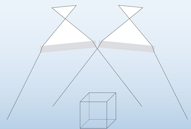
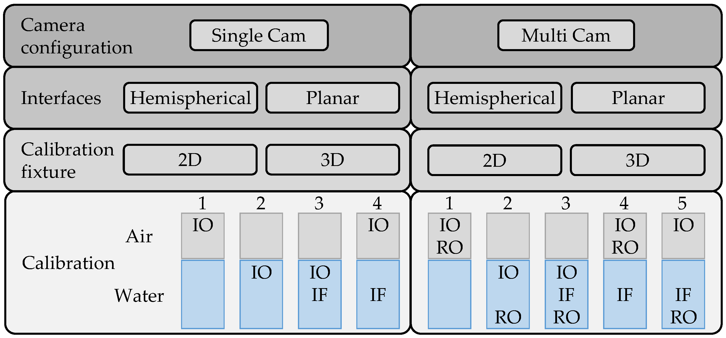
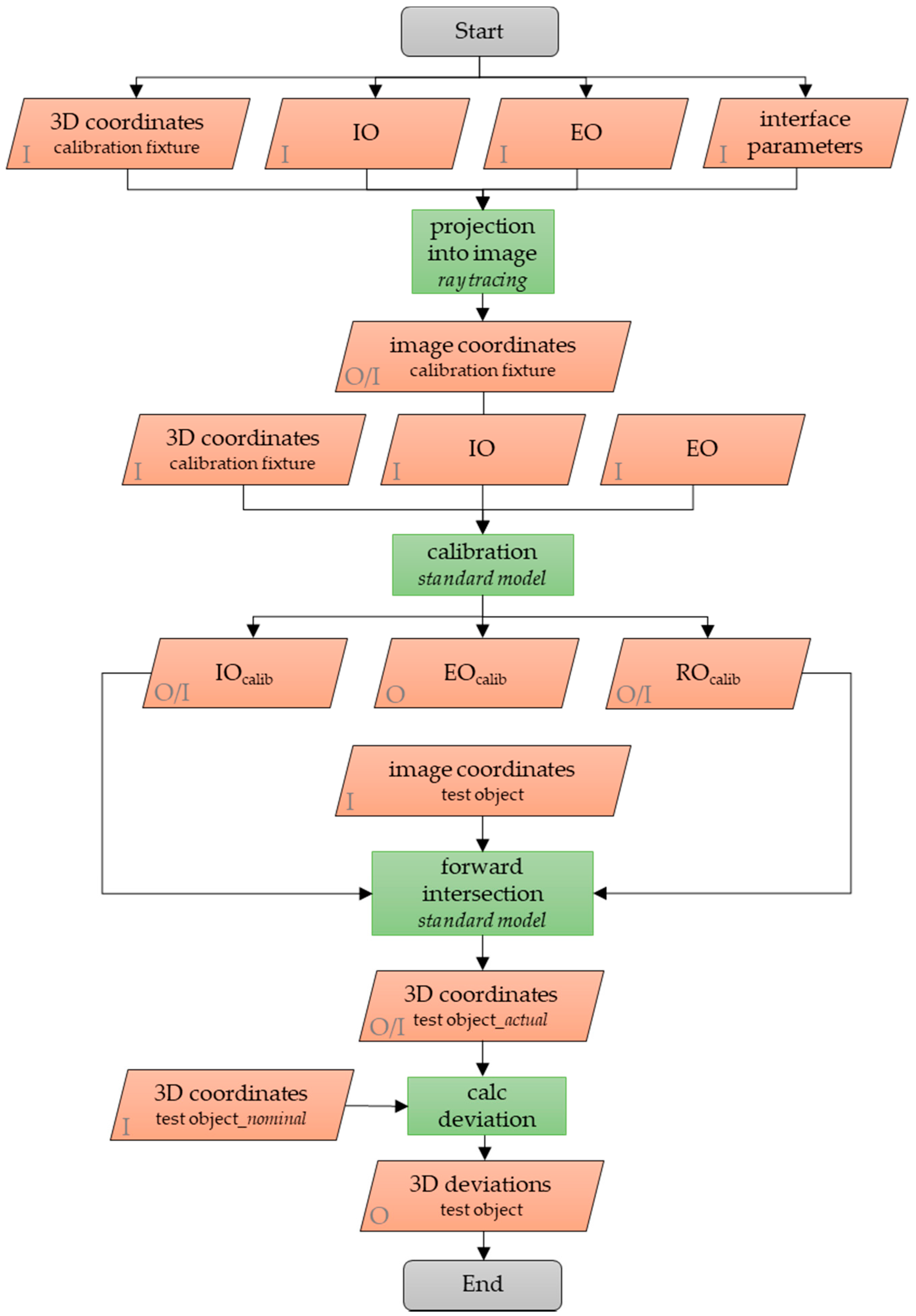
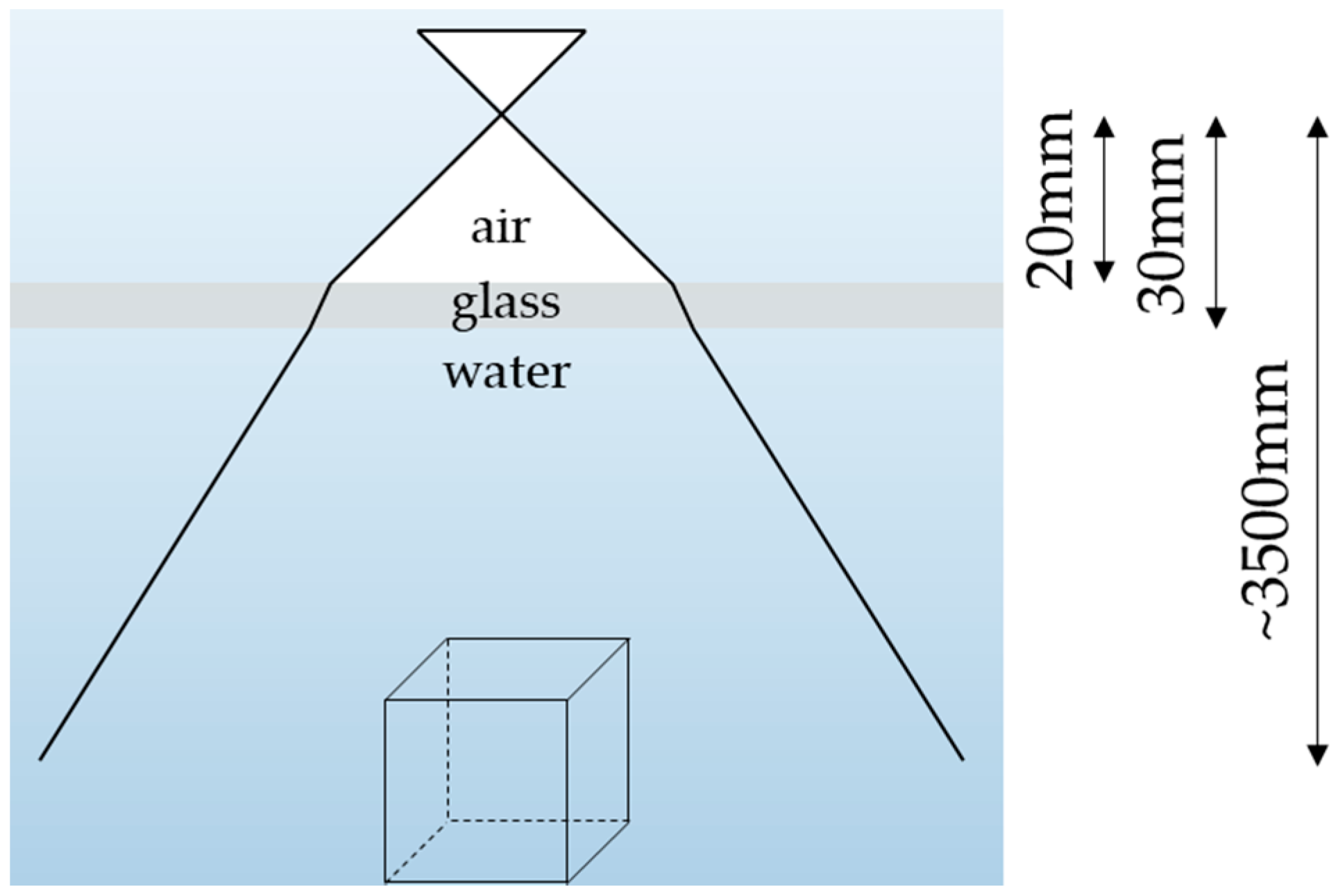
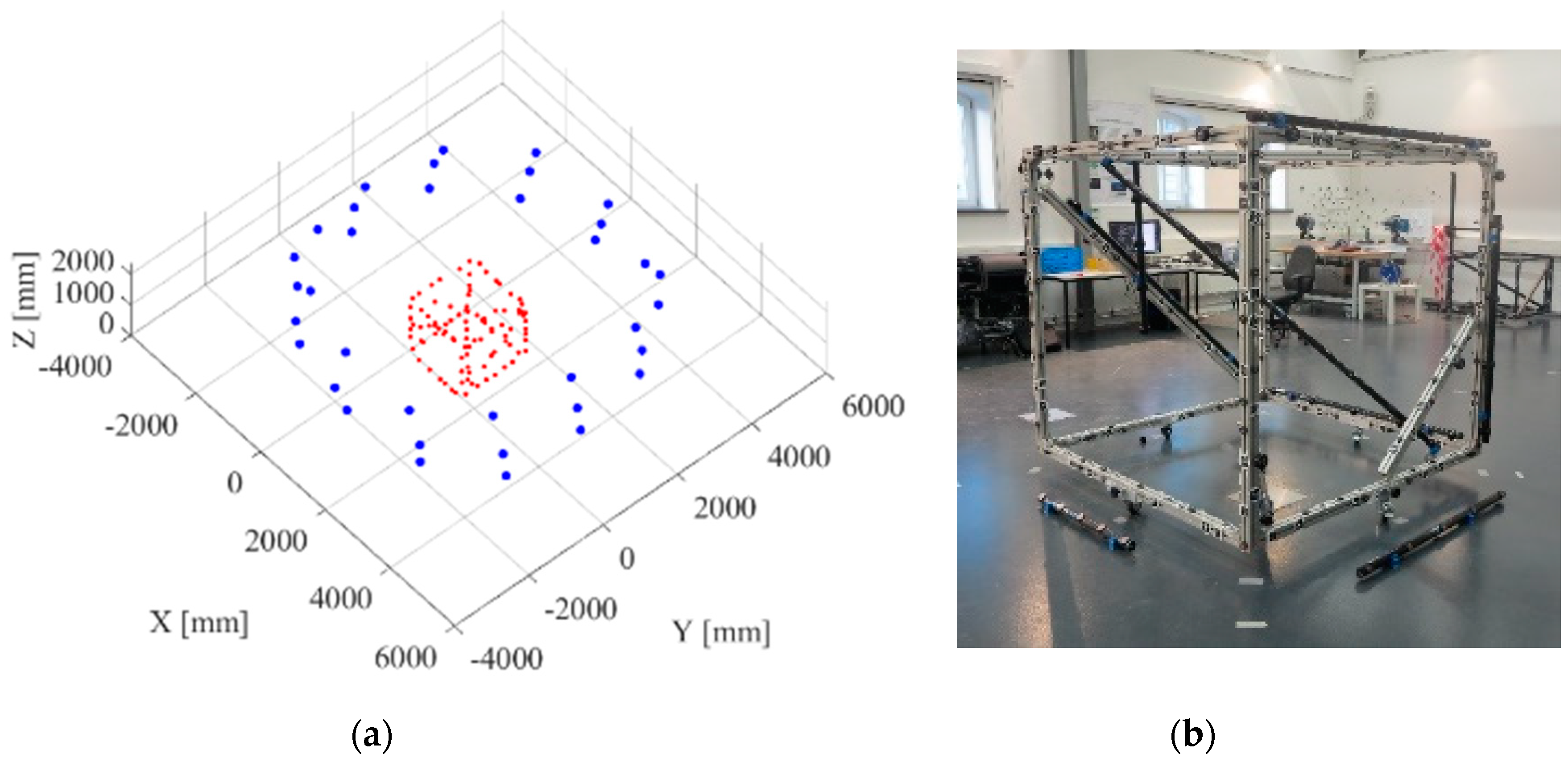
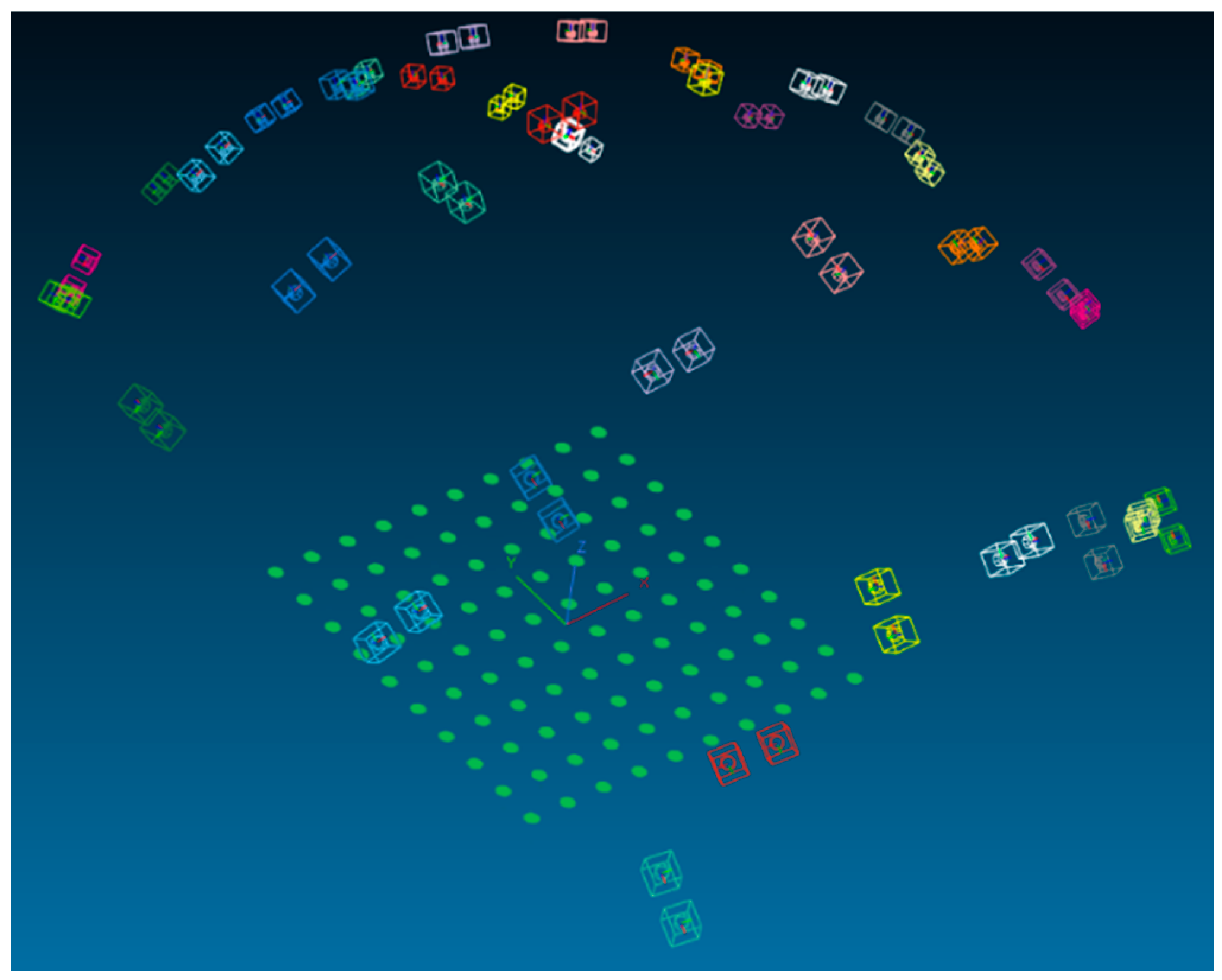
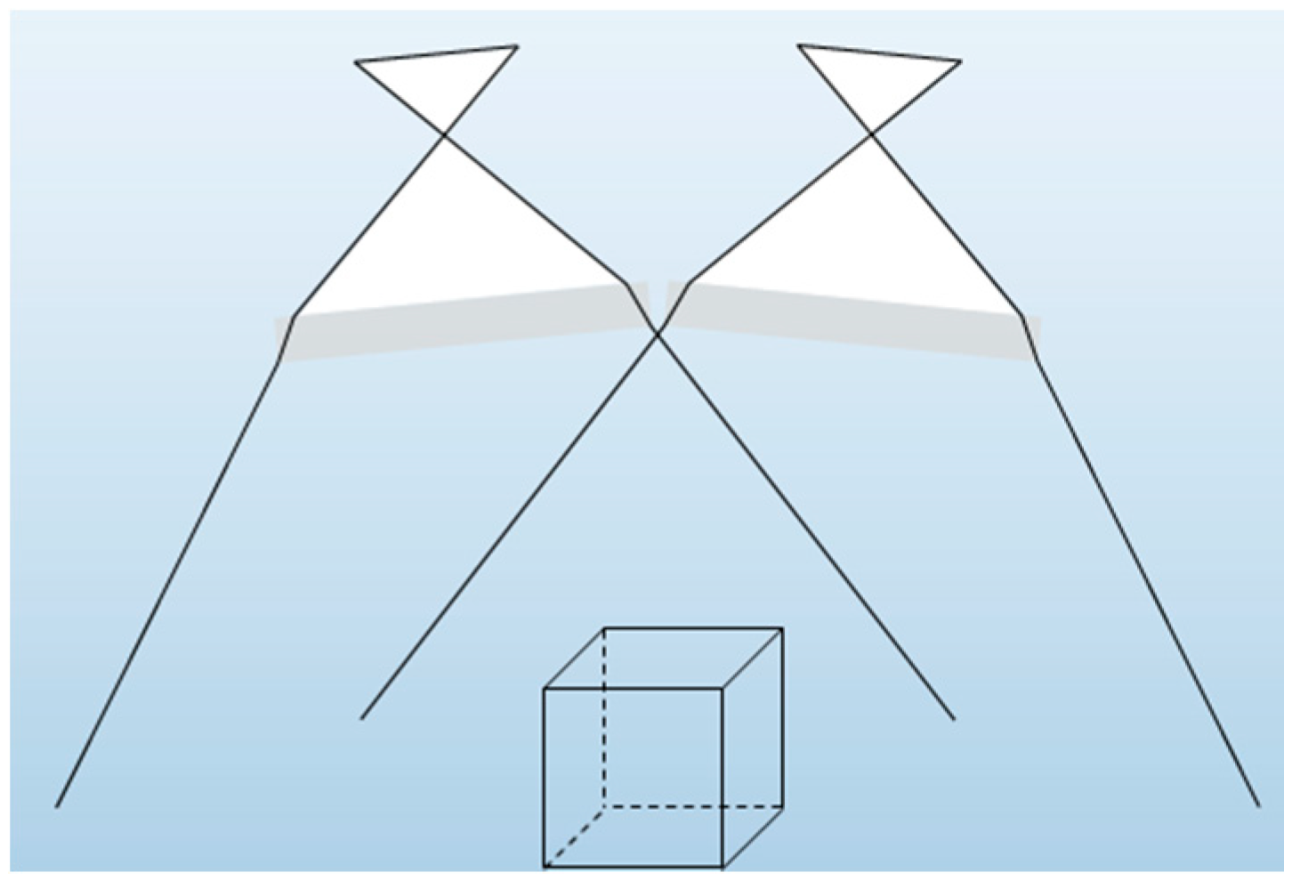
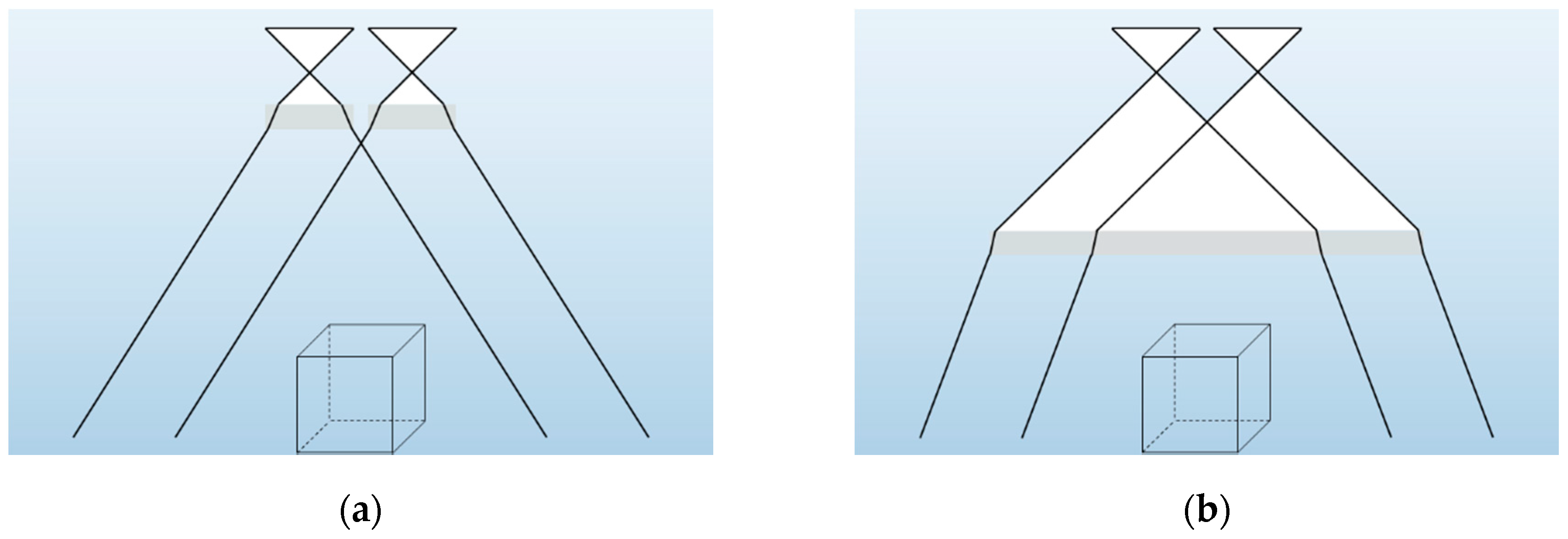
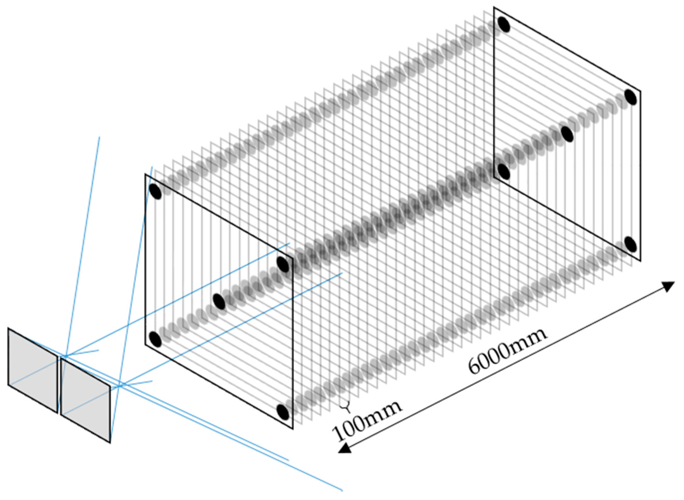
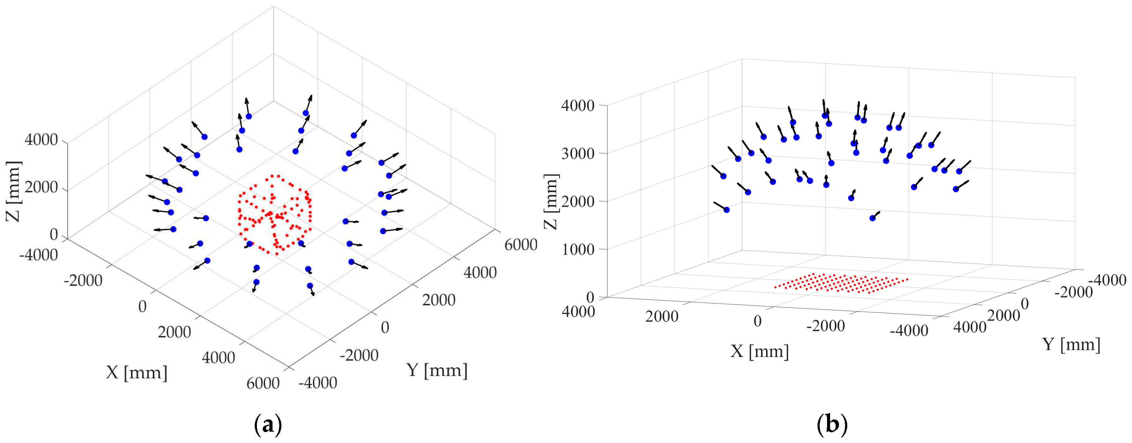
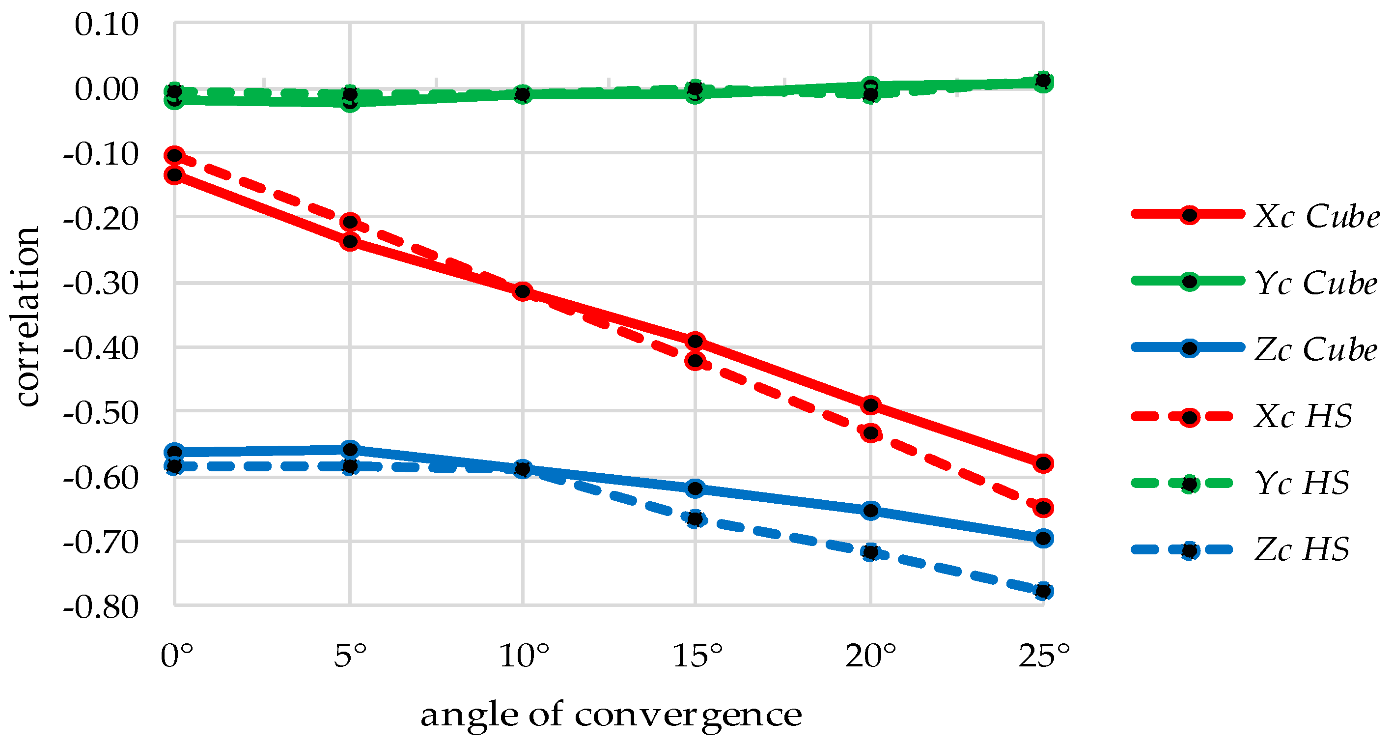
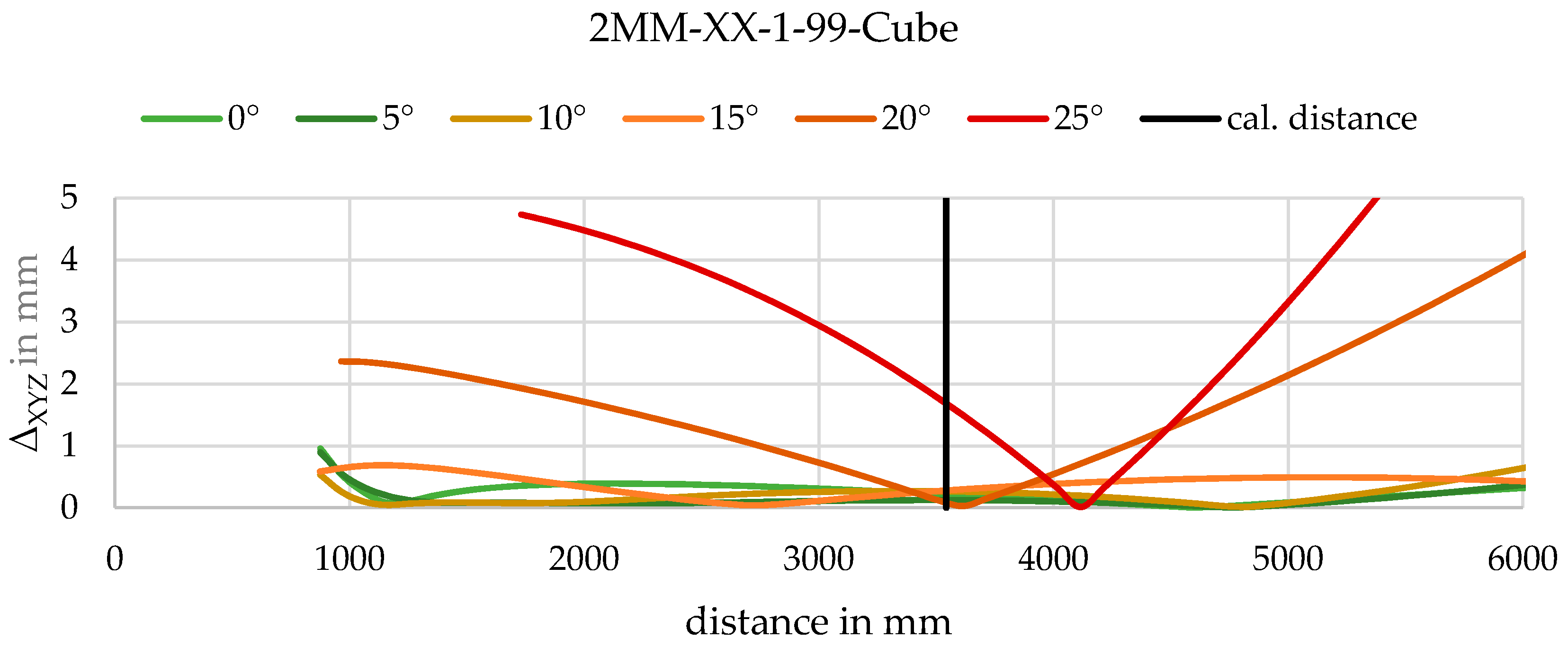
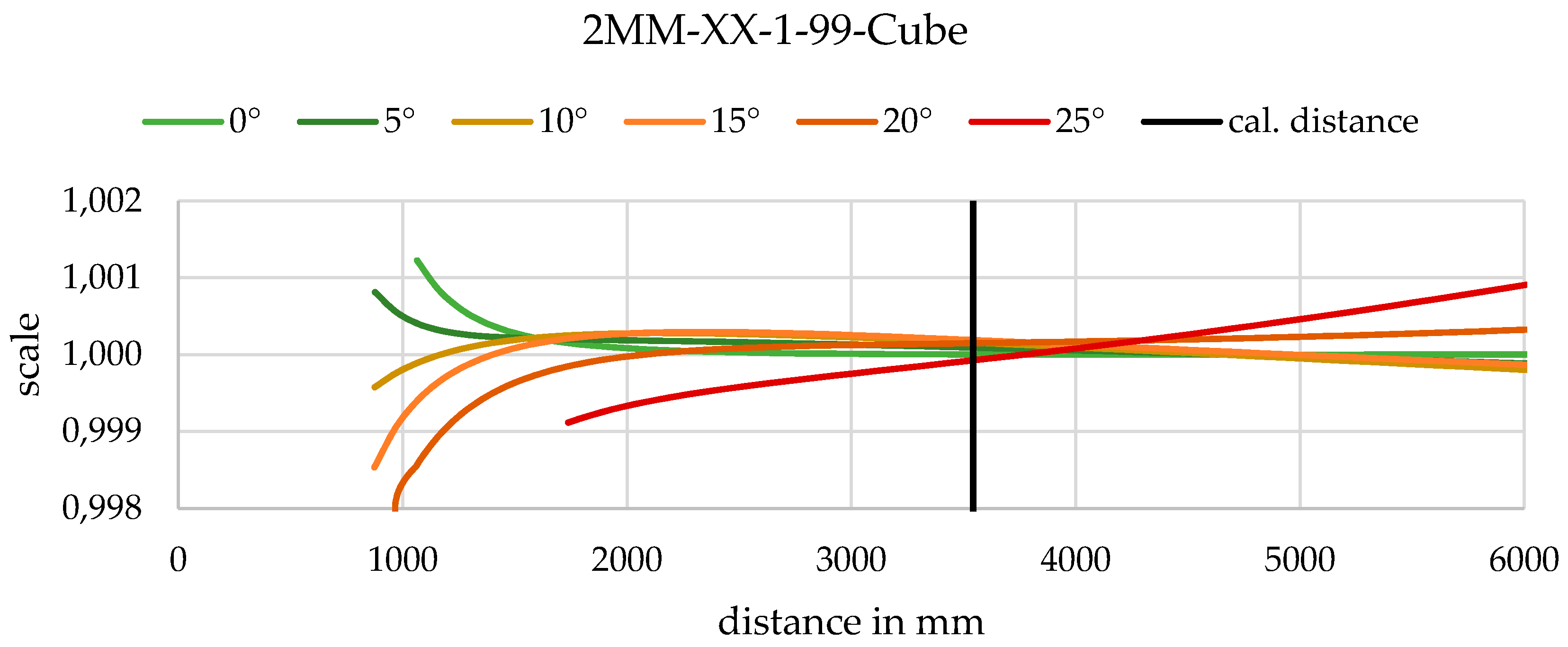
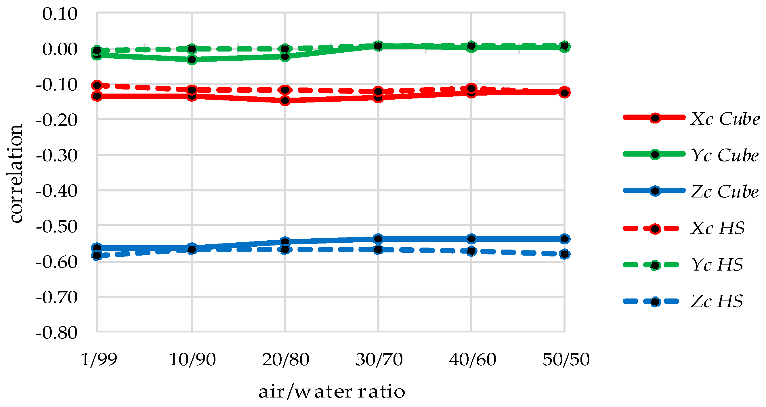
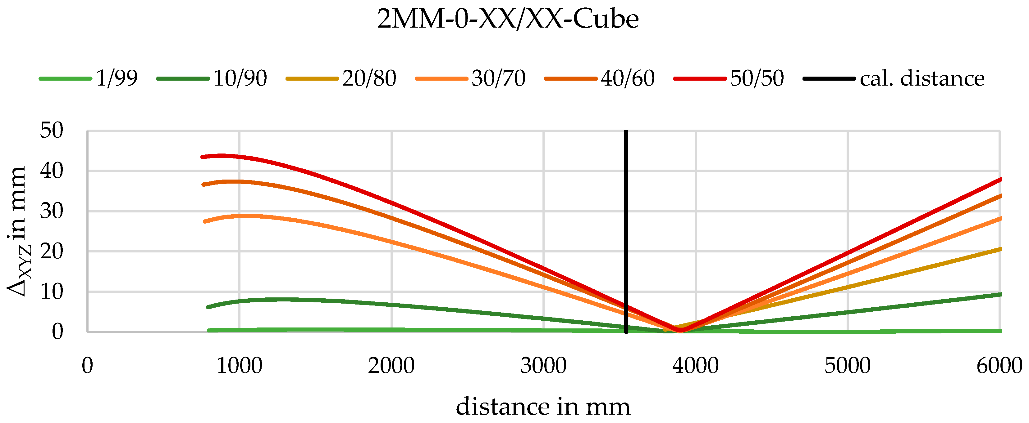
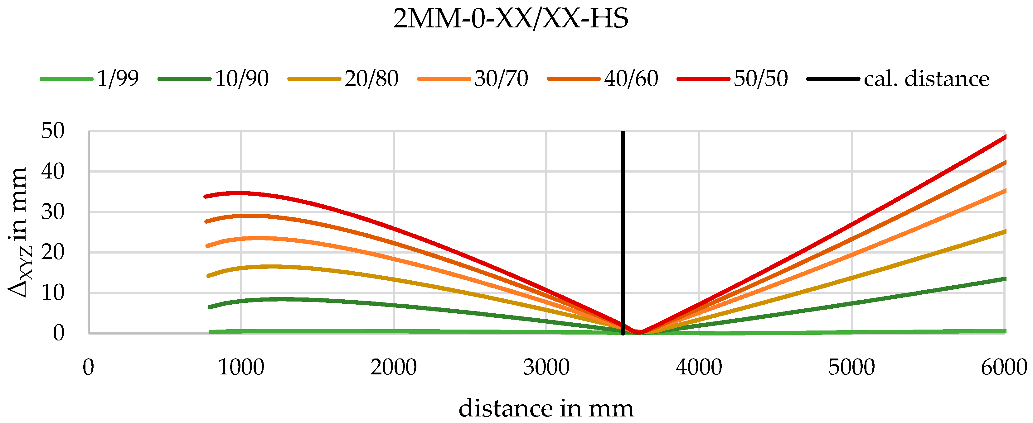
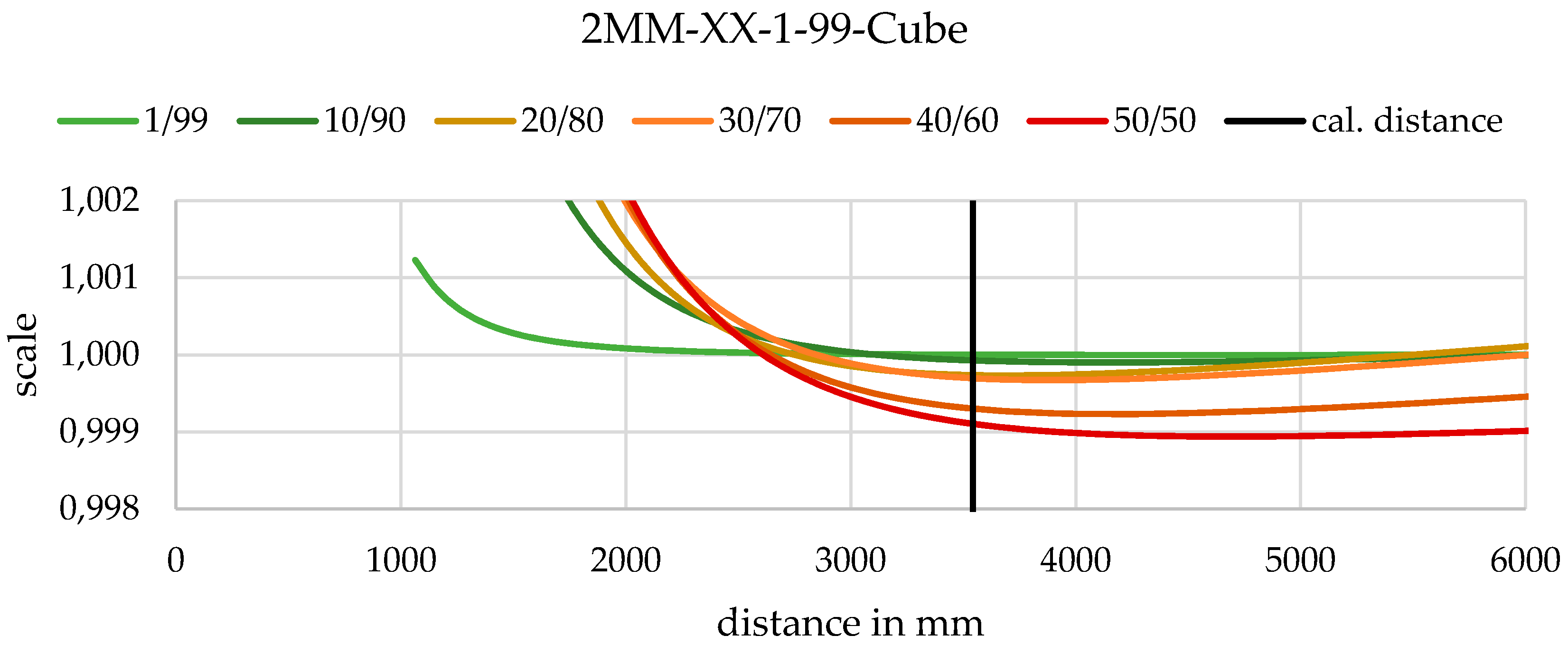
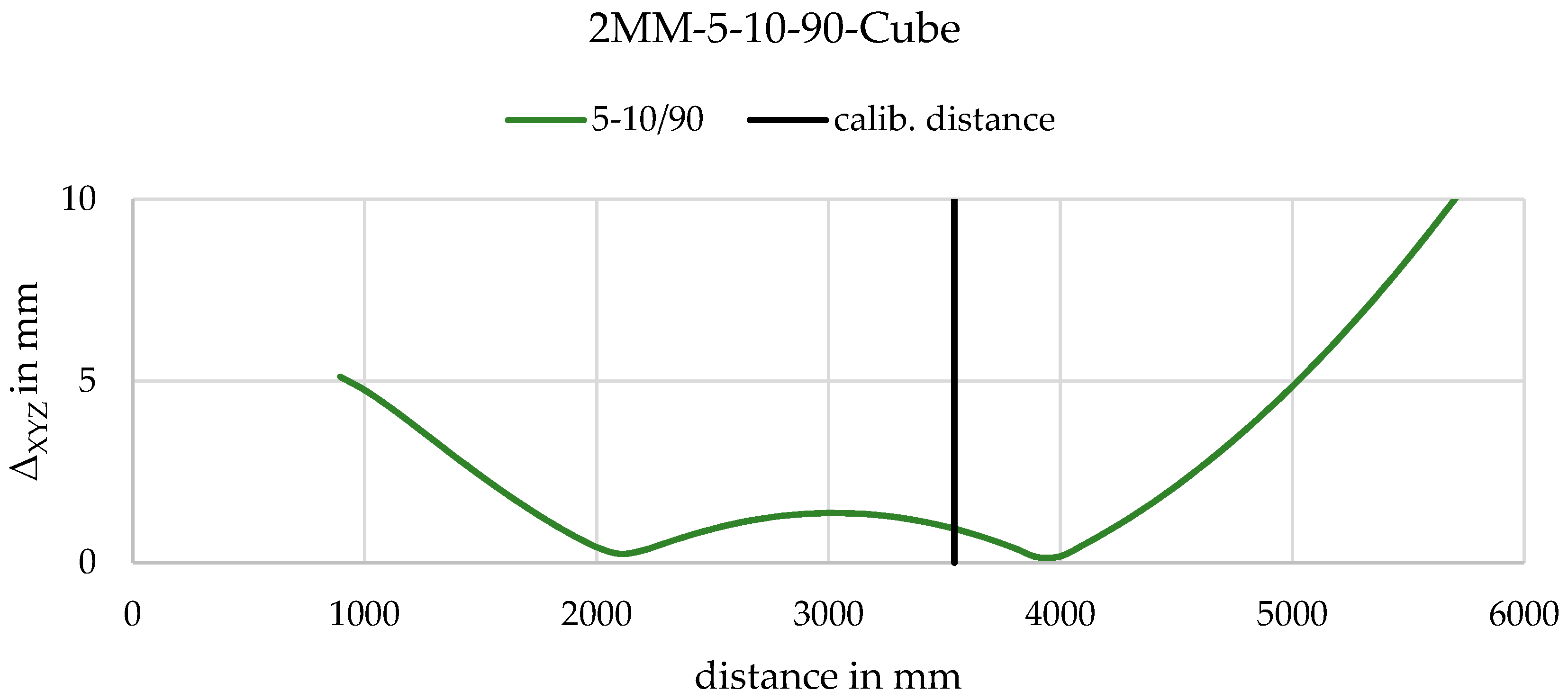
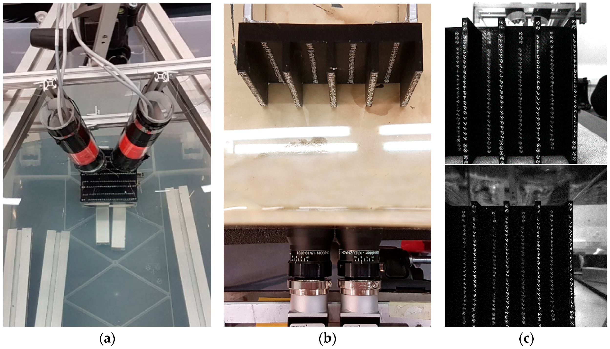
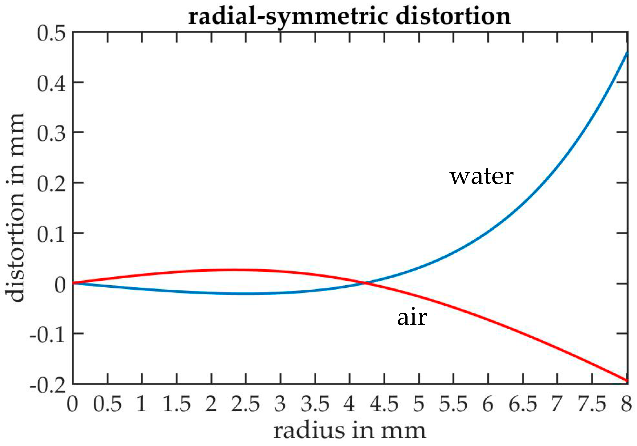
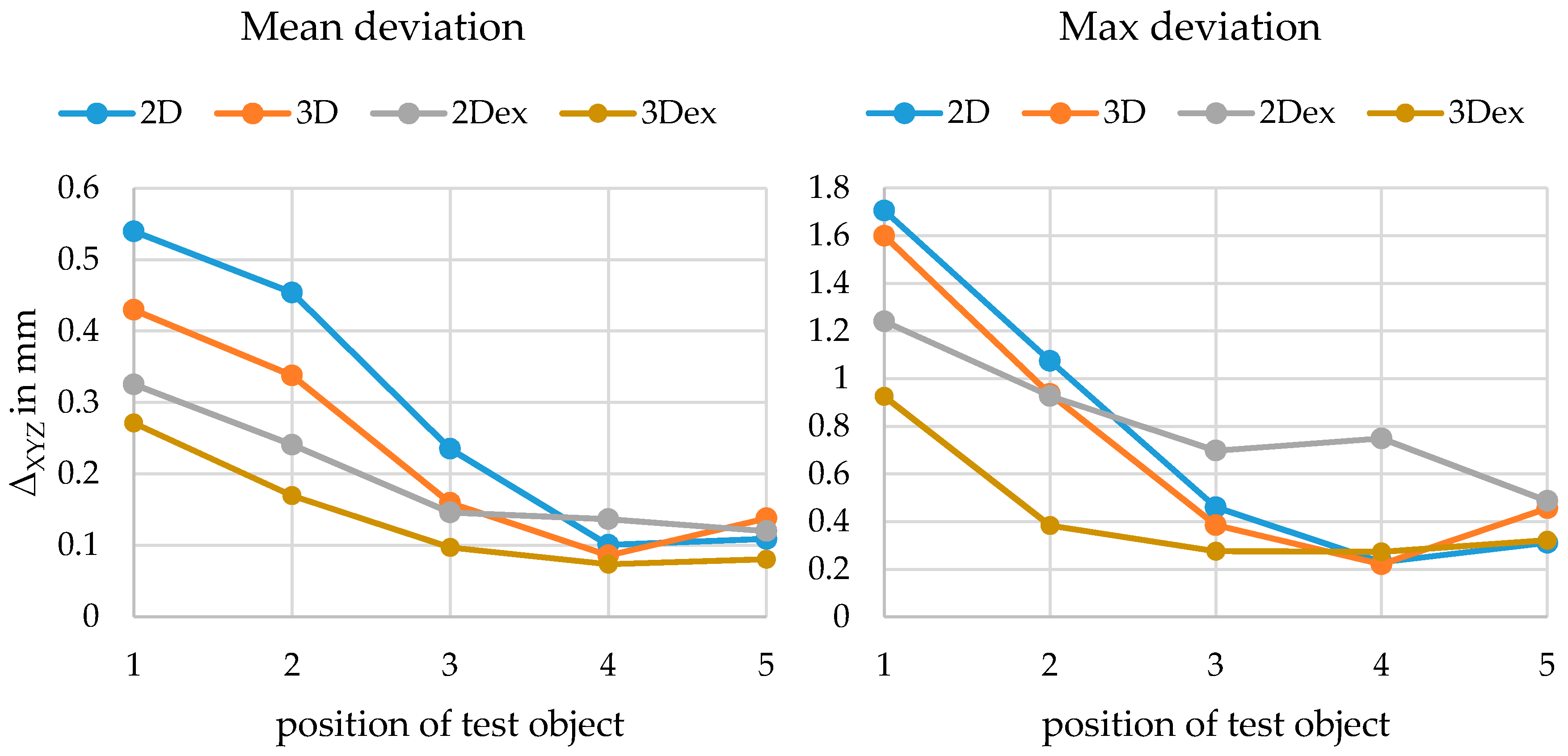
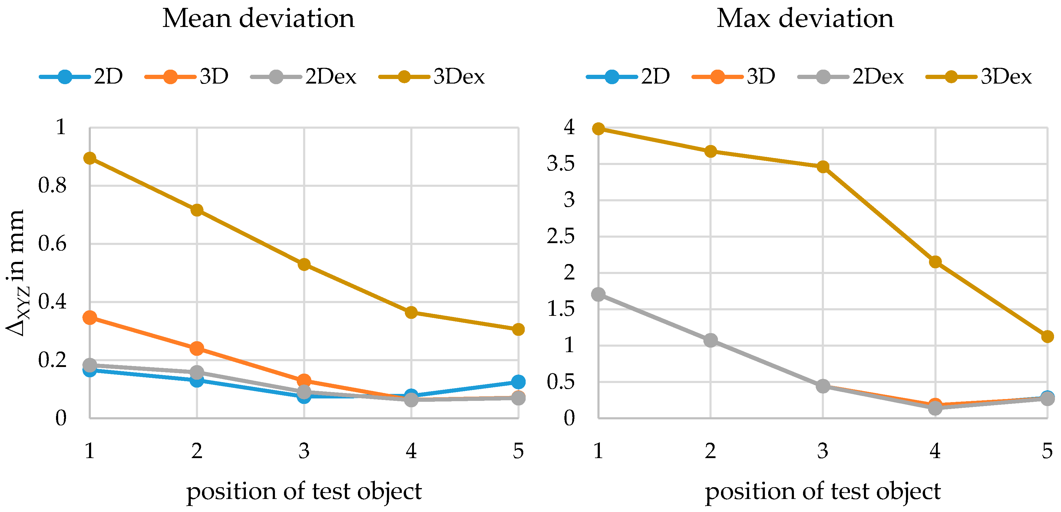
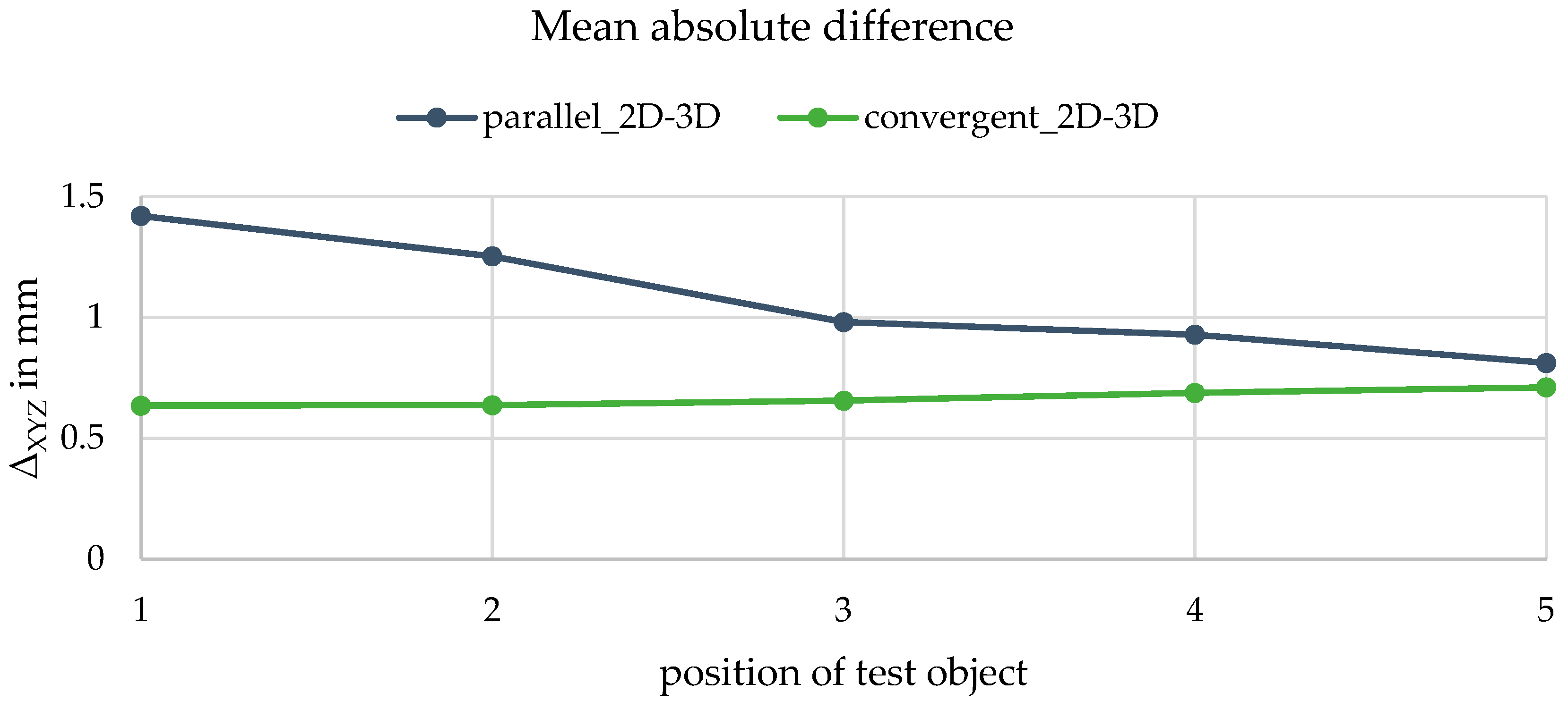
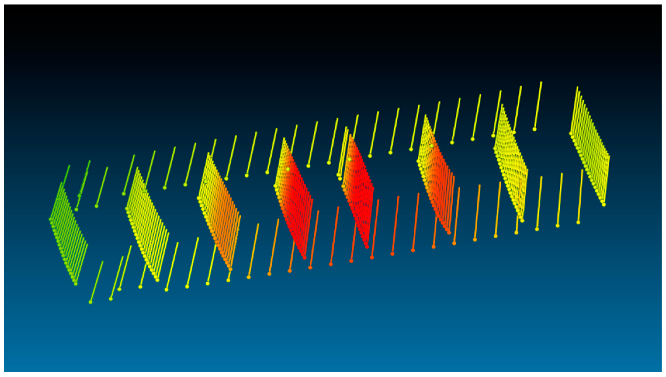
Table 1.
Simulated stereo datasets for different angles of convergence. The air/water ratio is not considered and named XX according to the notation (Section 3.1).
Table 1.
Simulated stereo datasets for different angles of convergence. The air/water ratio is not considered and named XX according to the notation (Section 3.1).
| Cube | HS |
|---|---|
| 2SM-0-Cube | 2SM-0-HS |
| 2MM-0-XX-Cube | 2MM-0-XX-HS |
| 2MM-5-XX-Cube | 2MM-5-XX-HS |
| 2MM-10-XX-Cube | 2MM-10-XX-HS |
| 2MM-15-XX-Cube | 2MM-15-XX-HS |
| 2MM-20-XX-Cube | 2MM-20-XX-HS |
| 2MM-25-XX-Cube | 2MM-25-XX-HS |
Table 2.
Simulated stereo datasets for different air/water ratios. The angle of convergence is not considered and named XX according to the notation (Section 3.1).
Table 2.
Simulated stereo datasets for different air/water ratios. The angle of convergence is not considered and named XX according to the notation (Section 3.1).
| Cube | HS |
|---|---|
| 2SM-XX-Cube | 2SM-XX-HS |
| 2MM-XX-1/99-Cube | 2MM-XX-1/99-HS |
| 2MM-XX-10/90-Cube | 2MM-XX-10/90-HS |
| 2MM-XX-20/80-Cube | 2MM-XX-20/80-HS |
| 2MM-XX-30/70-Cube | 2MM-XX-30/70-HS |
| 2MM-XX-40/60-Cube | 2MM-XX-40/60-HS |
| 2MM-XX-50/50-Cube | 2MM-XX-50/50-HS |
Table 3.
Interior orientation parameters (principal distance and radial distortion) of two single-medium and two multimedia datasets.
Table 3.
Interior orientation parameters (principal distance and radial distortion) of two single-medium and two multimedia datasets.
| No. | Experiment | Principal Distance c [mm] | A1 | A2 | A3 |
|---|---|---|---|---|---|
| 1 | nominal | −23.908 | 0.0 | 0.0 | 0.0 |
| 2 | 1SM-1/99-Cube | −23.908 | 0.0 | 0.0 | 0.0 |
| 3 | 1SM-1/99-HS | −23.908 | 0.0 | 0.0 | 0.0 |
| 4 | 1MM-1/99-Cube | −33.980 | 3.1e-4 | 1.4e-7 | 1.3e-10 |
| 5 | 1MM-1/99-HS | −33.979 | 3.1e-4 | 1.5e-7 | 1.1e-10 |
Table 4.
Relative orientation and principal distance of convergent datasets of Cube as a result of the bundle adjustment running standard software for different datasets with varying angles of convergence.
Table 4.
Relative orientation and principal distance of convergent datasets of Cube as a result of the bundle adjustment running standard software for different datasets with varying angles of convergence.
| No. | Dataset | Relative Orientation | c [mm] | |||||
|---|---|---|---|---|---|---|---|---|
| X0 [mm] | Y0 [mm] | Z0 [mm] | ω [°] | φ [°] | κ [°] | |||
| 0 | nominal | 200.000 | 0.000 | 0.000 | 0.000 | 0–25 | 0.000 | −23.908 |
| 1 | 2SM-0°-1/99-Cube | 200.000 | 0.000 | 0.000 | 0.000 | 0.000 | 0.000 | −23.908 |
| 2 | 2MM-0°-1/99-Cube | 199.994 | 0.000 | 0.019 | 0.000 | 0.000 | 0.000 | −33.979 |
| 3 | 2MM-5°-1/99-Cube | 200.572 | 0.000 | −0.062 | 0.000 | 5.001 | 0.000 | −33.978 |
| 4 | 2MM-10°-1/99-Cube | 201.143 | −0.002 | −0.116 | 0.000 | 10.000 | 0.000 | −33.978 |
| 5 | 2MM-15°-1/99-Cube | 201.715 | −0.007 | −0.192 | 0.000 | 15.003 | 0.000 | −33.979 |
| 6 | 2MM-20°-1/99-Cube | 202.266 | −0.010 | −0.339 | −0.001 | 20.003 | 0.000 | −33.979 |
| 7 | 2MM-25°-1/99-Cube | 202.884 | −0.011 | −0.378 | 0.001 | 25.004 | 0.000 | −33.981 |
Table 5.
Relative orientation and principal distance of convergent datasets of HS as a result of the bundle adjustment running standard software for different datasets with varying angles of convergence.
Table 5.
Relative orientation and principal distance of convergent datasets of HS as a result of the bundle adjustment running standard software for different datasets with varying angles of convergence.
| No. | Dataset | Relative Orientation | c [mm] | |||||
|---|---|---|---|---|---|---|---|---|
| X0 [mm] | Y0 [mm] | Z0 [mm] | ω [°] | φ [°] | κ [°] | |||
| 0 | nominal | 200.000 | 0.000 | 0.000 | 0.000 | 0–25 | 0.000 | −23.908 |
| 1 | 2SM-0°-1/99-HS | 200.000 | 0.000 | 0.000 | 0.000 | 0.000 | 0.000 | −23.908 |
| 2 | 2MM-0°-1/99-HS | 199.987 | 0.000 | 0.007 | 0.000 | 0.000 | 0.000 | −33.978 |
| 3 | 2MM-5°-1/99-HS | 200.573 | 0.000 | −0.047 | 0.000 | 5.000 | 0.000 | −33.977 |
| 4 | 2MM-10°-1/99-HS | 201.164 | −0.001 | −0.037 | 0.000 | 10.000 | 0.000 | −33.978 |
| 5 | 2MM-15°-1/99-HS | 201.736 | −0.004 | −0.082 | 0.000 | 15.000 | 0.000 | −33.979 |
| 6 | 2MM-20°-1/99-HS | 202.314 | −0.008 | −0.113 | 0.002 | 20.001 | 0.000 | −33.980 |
| 7 | 2MM-25°-1/99-HS | 202.845 | −0.005 | −0.290 | 0.001 | 25.000 | 0.000 | −33.981 |
Table 6.
Major correlations between selected interior and relative orientation parameters for dataset 2MM-25°-1/99-Cube and 2MM-25°-1/99-HS. Only correlations higher than |0.5| are listed. Grey cells indicate correlations lower than |0.5|.
Table 6.
Major correlations between selected interior and relative orientation parameters for dataset 2MM-25°-1/99-Cube and 2MM-25°-1/99-HS. Only correlations higher than |0.5| are listed. Grey cells indicate correlations lower than |0.5|.
| Parameter | Dataset | |||||||||
|---|---|---|---|---|---|---|---|---|---|---|
| Cube | HS | Cube | HS | Cube | HS | Cube | HS | Cube | HS | |
| X | −0.58 | −0.65 | ||||||||
| Y | ||||||||||
| Z | −0.69 | −0.78 | ||||||||
| ω | 0.75 | 0.81 | 0.76 | 0.80 | ||||||
| φ | −0.82 | −0.82 | −0.79 | −0.74 | ||||||
| κ | −0.88 | −0.90 | −0.85 | −0.87 | ||||||
| c | Xh | Yh | B1 | B2 | ||||||
Table 7.
Relative orientation and principal distance of ratio datasets of Cube as a result of the bundle adjustment running standard software for different datasets with varying air/water ratios.
Table 7.
Relative orientation and principal distance of ratio datasets of Cube as a result of the bundle adjustment running standard software for different datasets with varying air/water ratios.
| No. | Dataset | Relative Orientation | c [mm] | |||||
|---|---|---|---|---|---|---|---|---|
| X0 [mm] | Y0 [mm] | Z0 [mm] | ω [°] | Φ [°] | κ [°] | |||
| 0 | nominal | 200.000 | 0.000 | 0.000 | 0.000 | 0–25 | 0.000 | −23.908 |
| 1 | 2SM-0°-1/99-Cube | 200.000 | 0.000 | 0.000 | 0.000 | 0.000 | 0.000 | −23.908 |
| 2 | 2MM-0°-1/99-Cube | 199.994 | 0.000 | 0.019 | 0.000 | 0.000 | 0.000 | −33.979 |
| 3 | 2MM-0°-10/90-Cube | 199.912 | −0.018 | 0.012 | −0.001 | −0.008 | 0.001 | −33.891 |
| 4 | 2MM-0°-20/80-Cube | 199.780 | 0.021 | 1.491 | 0.003 | 0.018 | 0.001 | −33.806 |
| 5 | 2MM-0°-30/70-Cube | 199.732 | 0.142 | 1.501 | 0.019 | 0.002 | −0.002 | −33.744 |
| 6 | 2MM-0°-40/60-Cube | 199.664 | 0.219 | 1.594 | 0.018 | 0.015 | −0.001 | −33.654 |
| 7 | 2MM-0°-50/50-Cube | 199.702 | 0.234 | 2.345 | 0.021 | 0.033 | 0.000 | −33.549 |
Table 8.
Relative orientation and principal distance of ratio datasets of HS as a result of the bundle adjustment running standard software for different datasets with varying air/water ratios.
Table 8.
Relative orientation and principal distance of ratio datasets of HS as a result of the bundle adjustment running standard software for different datasets with varying air/water ratios.
| No. | Dataset | Relative Orientation | c [mm] | |||||
|---|---|---|---|---|---|---|---|---|
| X0 [mm] | Y0 [mm] | Z0 [mm] | ω [°] | Φ [°] | κ [°] | |||
| 0 | nominal | 200.000 | 0.000 | 0.000 | 0.000 | 0–25 | 0.000 | −23.908 |
| 1 | 2SM-0°-1/99-HS | 200.000 | 0.000 | 0.000 | 0.000 | 0.000 | 0.000 | −23.908 |
| 2 | 2MM-0°-1/99-HS | 199.987 | 0.000 | 0.007 | 0.000 | 0.000 | 0.000 | −33.978 |
| 3 | 2MM-0°-10/90-HS | 199.782 | −0.019 | 0.616 | −0.001 | 0.000 | 0.000 | −33.878 |
| 4 | 2MM-0°-20/80-HS | 199.586 | −0.039 | 1.288 | −0.004 | 0.004 | 0.000 | −33.758 |
| 5 | 2MM-0°-30/70-HS | 199.441 | −0.056 | 2.092 | −0.006 | 0.007 | 0.000 | −33.630 |
| 6 | 2MM-0°-40/60-HS | 199.345 | −0.028 | 2.187 | −0.003 | 0.011 | 0.000 | −33.496 |
| 7 | 2MM-0°-50/50-HS | 199.287 | −0.028 | 2.254 | −0.001 | 0.013 | 0.000 | −33.362 |
Table 9.
Major correlations between selected interior and relative orientation parameters for dataset 2MM-0°-50/50-Cube and 2MM-0°-50/50-HS. Only correlations bigger than |0.5| are listed. Grey cells indicate correlations less than |0.5|.
Table 9.
Major correlations between selected interior and relative orientation parameters for dataset 2MM-0°-50/50-Cube and 2MM-0°-50/50-HS. Only correlations bigger than |0.5| are listed. Grey cells indicate correlations less than |0.5|.
| Parameter | Dataset | |||||||||
|---|---|---|---|---|---|---|---|---|---|---|
| Cube | HS | Cube | HS | Cube | HS | Cube | HS | Cube | HS | |
| X | ||||||||||
| Y | ||||||||||
| Z | −0.54 | −0.58 | ||||||||
| ω | 0.55 | 0.63 | 0.54 | 0.63 | ||||||
| φ | −0.64 | −0.64 | −0.64 | −0.62 | ||||||
| κ | ||||||||||
| c | Xh | Yh | B1 | B2 | ||||||
Table 10.
Relative orientation as a result of the multimedia bundle adjustment for the most critical datasets.
Table 10.
Relative orientation as a result of the multimedia bundle adjustment for the most critical datasets.
| No. | Dataset | Relative Orientation | |||||
|---|---|---|---|---|---|---|---|
| X0 [mm] | Y0 mm] | Z0 [mm] | ω [°] | φ [°] | κ [°] | ||
| 0 | nominal | 200.000 | 0.000 | 0.000 | 0.000 | 0–25 | 0.000 |
| 1 | 2MM-25°-1/99-Cube | 200.000 | 0.000 | 0.000 | 0.000 | 25.000 | 0.000 |
| 2 | 2MM-0°-50/50-Cube | 200.000 | 0.000 | 0.000 | 0.000 | 0.000 | 0.000 |
| 3 | 2MM-25°-50/50-Cube | 200.000 | 0.000 | 0.000 | 0.000 | 0.000 | 0.000 |
Table 11.
Interior orientation parameters and their standard deviation of the left camera of the bundle adjustment using standard software in the air and in the underwater configuration (exemplary for the parallel setup, 3D calibration fixture used).
Table 11.
Interior orientation parameters and their standard deviation of the left camera of the bundle adjustment using standard software in the air and in the underwater configuration (exemplary for the parallel setup, 3D calibration fixture used).
| Data | c | xh | yh | A1 | A2 | A3 | B1 | B2 | C1 | C2 |
|---|---|---|---|---|---|---|---|---|---|---|
| [mm] | [mm] | [mm] | ||||||||
| σc | σxh | σyh | σA1 | σA2 | σA3 | σB1 | σB2 | σC1 | σC2 | |
| IO AIR | −10.52 | −6.84E-02 | −4.24E-02 | −1.13E-03 | 1.04E-05 | −4.45E-08 | −4.08E-05 | −3.79E-05 | −1.83E-04 | −6.51E-05 |
| 1.08E-03 | 7.43E-04 | 7.96E-04 | 4.88E-06 | 2.25E-07 | 3.18E-09 | 2.50E-06 | 2.02E-06 | 1.16E-05 | 1.15E-05 | |
| IO Water | −14.49 | −4.41E-02 | −3.01E-02 | 6.35E-04 | 2.64E-06 | 6.87E-08 | 4.62E-05 | −1.34E-05 | −1.30E-04 | −2.02E-04 |
| 3.07E-03 | 2.73E-03 | 2.85E-03 | 9.32E-06 | 4.41E-07 | 6.31E-09 | 8.22E-06 | 8.39E-06 | 2.53E-05 | 3.09E-05 |
Table 12.
The relative orientation of the bundle adjustment using standard software (implicit modelling) and own implementation (explicit modelling). The ending 2D/3D indicates which calibration fixture is used. The ending “ex” indicates the explicitly modelled data.
Table 12.
The relative orientation of the bundle adjustment using standard software (implicit modelling) and own implementation (explicit modelling). The ending 2D/3D indicates which calibration fixture is used. The ending “ex” indicates the explicitly modelled data.
| No. | Dataset | Relative Orientation | c [mm] | |||||
|---|---|---|---|---|---|---|---|---|
| X0 [mm] | Y0 [mm] | Z0 [mm] | ω [°] | Φ [°] | κ [°] | |||
| 0 | air, parallel | −37.914 | 0.886 | 0.214 | 0.120 | −0.022 | −0.180 | −10.520 |
| 1 | parallel-2D | −37.817 | 0.916 | 0.251 | 0.197 | 0.040 | −0.194 | −14.547 |
| 2 | parallel-3D | −37.814 | 0.939 | 0.510 | 0.139 | 0.022 | −0.180 | −14.492 |
| 3 | parallel-2Dex | −37.544 | 0.838 | 0.940 | 0.079 | −0.053 | −0.197 | −10.520 |
| 4 | parallel-3Dex | −37.744 | 0.935 | 0.450 | 0.080 | 0.069 | −0.193 | −10.520 |
| 5 | convergent-2D | −75.961 | −2.683 | −17.026 | 2.461 | −27.792 | −2.859 | −14.555 |
| 6 | convergent-3D | −75.611 | −2.735 | −16.769 | 2.452 | −27.556 | −2.862 | −14.501 |
| 7 | convergent-2Dex | −72.735 | −2.602 | −15.273 | 2.446 | −27.334 | −2.846 | −10.520 |
| 8 | convergent-3Dex | −74.194 | −4.169 | 5.248 | 3.285 | −28.640 | −2.828 | −10.520 |
© 2020 by the authors. Licensee MDPI, Basel, Switzerland. This article is an open access article distributed under the terms and conditions of the Creative Commons Attribution (CC BY) license (http://creativecommons.org/licenses/by/4.0/).
Share and Cite
MDPI and ACS Style
Kahmen, O.; Rofallski, R.; Luhmann, T. Impact of Stereo Camera Calibration to Object Accuracy in Multimedia Photogrammetry. Remote Sens. 2020, 12, 2057. https://0-doi-org.brum.beds.ac.uk/10.3390/rs12122057
AMA Style
Kahmen O, Rofallski R, Luhmann T. Impact of Stereo Camera Calibration to Object Accuracy in Multimedia Photogrammetry. Remote Sensing. 2020; 12(12):2057. https://0-doi-org.brum.beds.ac.uk/10.3390/rs12122057
Chicago/Turabian StyleKahmen, Oliver, Robin Rofallski, and Thomas Luhmann. 2020. "Impact of Stereo Camera Calibration to Object Accuracy in Multimedia Photogrammetry" Remote Sensing 12, no. 12: 2057. https://0-doi-org.brum.beds.ac.uk/10.3390/rs12122057
Note that from the first issue of 2016, this journal uses article numbers instead of page numbers. See further details here.