Article

Towards a Large-Scale 3D Modeling of the Built Environment—Joint Analysis of TanDEM-X, Sentinel-2 and Open Street Map Data

1
German Aerospace Center (DLR), Earth Observation Center (EOC), German Remote Sensing Data Center (DFD), Oberpfaffenhofen, D-82234 Weßling, Germany
2
European Space Agency (ESA), Directorate of Earth Observation Programmes, Future Systems Department, Φ-lab Explore, ESRIN, Via Galileo Galilei, 64 I-00044 Casella Postale, Frascati, Italy
*
Author to whom correspondence should be addressed.
Remote Sens. 2020, 12(15), 2391; https://0-doi-org.brum.beds.ac.uk/10.3390/rs12152391
Submission received: 26 June 2020 / Revised: 20 July 2020 / Accepted: 23 July 2020 / Published: 25 July 2020

Abstract

:
Continental to global scale mapping of the human settlement extent based on earth observation satellite data has made considerable progress. Nevertheless, the current approaches only provide a two-dimensional representation of the built environment. Therewith, a full characterization is restricted in terms of the urban morphology and built-up density, which can only be gained by a detailed examination of the vertical settlement extent. This paper introduces a methodology for the extraction of three-dimensional (3D) information on human settlements by analyzing the digital elevation and radar intensity data collected by the German TanDEM-X satellite mission in combination with multispectral Sentinel-2 imagery and data from the Open Street Map initiative and the Global Urban Footprint human settlement mask. The first module of the underlying processor generates a normalized digital surface model from the TanDEM-X digital elevation model for all regions marked as a built-up area by the Global Urban Footprint. The second module generates a building mask based on a joint processing of Open Street Map, TanDEM-X/TerraSAR-X radar images, the calculated normalized digital surface model and Sentinel-2 imagery. Finally, a third module allocates the local relative heights of the normalized digital surface model to the building structures provided by the building mask. The outcome of the procedure is a 3D map of the built environment showing the estimated local height for all identified vertical building structures at 12 m spatial resolution. The results of a first validation campaign based on reference data collected for the seven cities of Amsterdam (NL), Indianapolis (US), Kigali (RW), Munich (DE), New York (US), Vienna (AT), and Washington (US) indicate the potential of the proposed methodology to accurately estimate the distribution of building heights within the built-up area.

1. Introduction

Global urbanization poses a considerable challenge to the goal of sustainable urban development. According to recent estimates of the United Nations [1], about 70% of the world’s population will live in cities by 2050. By that time, it is expected that 90% of population growth, 80% of the increase in wealth and approximately 60% of energy consumption will occur in urban areas. This unprecedented rise of cities and urbanized areas demands for efforts to be made in the integration of new strategies that can help to achieve economic growth as well as social equality and stability, while protecting the environment and reducing the effects and impacts of climate change [2].
To this end, understanding and monitoring the changes in the size and composition of the built environment has become a central element of political frameworks. Here, up-to-date and globally consistent data on the status and characteristics of the built-up area is at the core of national and local initiatives focusing on sustainable development [3,4,5,6]. However, due to the dynamic and rapid nature of global urbanization, such data (and derived empirical evidence) are a resource which is still rare. Here, earth observation (EO) has already been successfully employed to globally identify human settlements and to delineate their size in term of their horizontal extent. Different authors, for instance, introduce various methodologies for the extraction of human settlements, describing the built-area as urban/rural, built-up/non-built-up, or in terms of the population counts per settlement area [7,8,9,10,11,12]. Moreover, human settlements are further characterized in relation to the percentage of impervious surfaces within the built-up area, allowing—to a certain degree—for an assessment of the built-up density and its corresponding population [13,14,15,16].
While the datasets resulting from these approaches have been used in a wide range of applications, remaining limitations still arise from the fact that they only represent a two-dimensional (2D) mapping of the settlement characteristics in the horizontal dimension. In other words, any detailed and effective examinations of the built-up environment in terms of the volume or floor space (as the optimal measure for built-up density), urban morphology, or population distribution, inevitably require the consideration of the vertical dimension. In this context, precise studies on the three-dimensional (3D) extent of urban structures at the level of single cities have been frequently reported in recent years, with many approaches relying on digital elevation data derived from very high-resolution aerial and satellite imagery or airborne light detection and ranging (LiDAR) data [16,17,18,19,20,21]. Another interesting approach is Synthetic Aperture Radar (SAR) tomography which uses data from spaceborne imaging radar systems to reconstruct the location and height of buildings at a very high spatial resolution [22]. However, so far this method has only been applied in studies at a city or regional scale, mostly due to the quite comprehensive data stacks required.
First approaches suitable of measuring the status and development of vertical expansion at a large-scale have been introduced by Frolking et al. [23] and Mahendra and Seto [6]. In order to quantify the outward and upward expansion of cities worldwide, both studies analyze data on the backscattering intensity of the built-up environment derived from NASA’s SeaWinds microwave scatterometer in combination with information from nightlight data and the Global Human Settlement Layer, respectively. Similarly, Mathews et al. [24] estimated the built-up volume for selected cities at a 1km resolution based on scatterometer data collected by QuikSCAT. While promising, these approaches still suffer limitations arising from the comparably low spatial resolution of the scatterometer data and from the fact that variations in the backscattering intensity can result from a multitude of effects in addition to the size and vertical growth of buildings.
Alternative large-scale approaches follow the already established standard idea of defining the local 3D built-up structure via a normalized digital surface model (nDSM), which is calculated by subtracting a modeled digital terrain model (DTM) from the original digital surface model (DSM). Marconcini et al. [25] demonstrated an approach to derive building heights at a spatial resolution of ~100 m with morphological operations that are applied to globally available DSMs such as the 12 m TanDEM-X digital elevation model (TDX-DEM). The same method was later employed by Clinton et al. [26] to conduct a worldwide estimation of built-up heights from the 30 m data of the AW3D30 DSM. Geiß et al. [27] used the TDX-DEM elevation data in combination with Sentinel-2 imagery to estimate the built-up height and density for selected urban areas. Recently, Li et al. [28] presented an approach for the mapping and analysis of 3D building structures based on random forest models applied to a large collection of earth observation data to produce maps of 3D building structures for China, Europe and the United States.
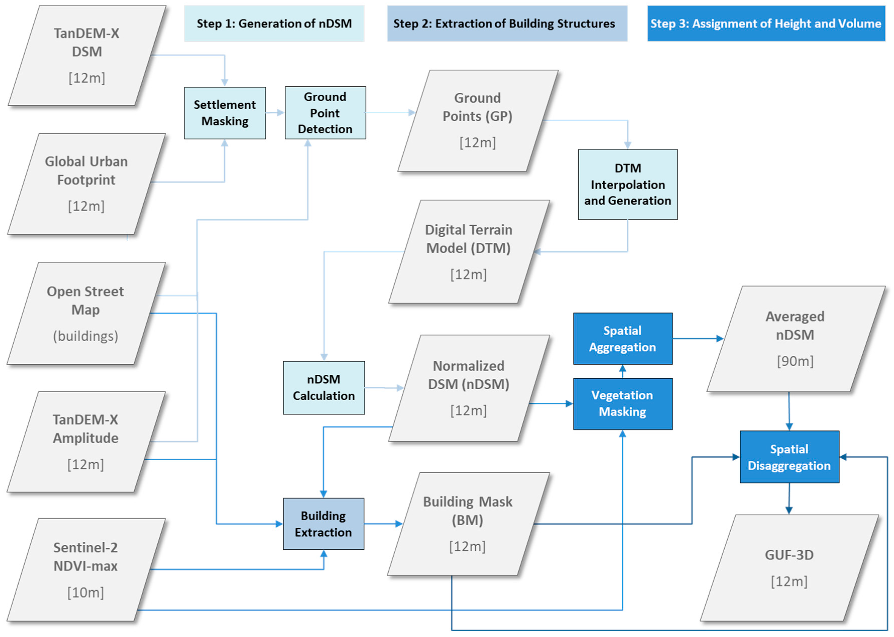
However, none of the approaches developed so far have yet been used to generate a spatially detailed map (<30 m spatial resolution) of the small-scale 3D building structures at a continental or global scale. Hence, this paper presents a processing and analytics concept aiming for a high-resolution large-scale 3D mapping of human settlements. The approach is based on a joint analysis of data collected by the German TanDEM-X satellite mission, namely the TanDEM-X digital elevation model (TDX-DEM) and the underlying SAR amplitude images (TDM-AMP). In addition, multispectral Sentinel-2 (S2) imagery, Open Street Map data (OSM), and the Global Urban Footprint (GUF) settlement mask are considered in this multi-source data analytics procedure.
Section 2 of this manuscript first outlines the input data sources, followed by a detailed description of the main components of the processing framework for urban 3D mapping. This includes automated workflows for (i) the calculation of an nDSM, (ii) the generation of a building mask, and (iii) the assignment of heights to the building structures provided by the building mask. Section 3 then specifies the basic properties of the resulting Global Urban Footprint 3D (GUF-3D) data product along with the first results of a validation exercise conducted on the basis of reference data collected for the cities of Amsterdam (NL), Indianapolis (US), Kigali (RW), Munich (DE), New York (US), Vienna (AT), and Washington (US). Finally, the conclusions are drawn and an outlook on the next developments is provided in Section 4.

2. Three-Dimensional Analysis of the Built-Up Area

The technical framework to generate large-area 3D built-up maps is based on a suite of orchestrated workflows for a highly automated management, processing and analysis of mass geodata. Here, the related solutions capitalize on key knowledge, technologies and data that the study team has already successfully developed and operationally deployed in the context of global urban observation and monitoring, including the Global Urban Footprint (GUF) [29], TimeScan [30], and the World Settlement Footprint 2015 (WSF 2015) [12].

2.1. Input Data Sources

A key element of the GUF-3D analysis is a multi-source information analysis based on a systematic exploitation of data collections from earth observation (EO) and volunteered geographic information (VGI). The primary data source for the 3D modeling was the TanDEM-X digital elevation model (TDX-DEM). The TDX-DEM is currently the most accurate global digital elevation model (DEM) available. It was derived from single-pass SAR interferometry based on the twin X-band satellites TerraSAR-X and TanDEM-X in the context of the German TanDEM-X mission [31]. The SAR data used for the global DEM production were acquired between December 2010 and January 2015 in StripMap mode (3 m posting) with horizontal transmit and receive polarization. The TDX-DEM shows a 0.4 arcsec posting (~12 m) with a 10 m absolute height accuracy (90% linear error) and 2–4 m relative accuracy depending on the terrain slope [32]. The relative height accuracy of 4 m is already in a range that potentially allows for the accurate determination of the number of floors of a building. The absolute height accuracy of 10 m is a less critical factor than the intended approach being based on the analysis of relative height differences using an nDSM. However, the 12 m horizontal resolution of the TDX-DEM still presents a challenge with respect to an accurate detection of buildings or at least the related small-scale morphologic and structural patterns.
To compensate for this limitation, the developed approach employs a multi-source data analytics procedure that integrates information on the location of building structures from two additional sources. Wherever available, all objects tagged as buildings in Open Street Map (OSM) [33] were used to mark the position and extent of buildings, for which, in a later step, the height was estimated from the TDX-DEM. However, although nominally available at a global scale, the data quality, consistency and completeness significantly differ from place to place. Thus, in all areas where no OSM building data was available, the local radar backscattering characteristics derived from TDX-AMP (radar amplitude images) were used to delineate potential building structures. For this purpose, the 3 m StripMap TDX-AMP images already used for the GUF production [7] were transferred to the 12 m posting of the TDX-DEM by means of a spatial averaging operation as described by Wendleder et al. [34].
To spatially delimit the analyses on settlements only, the GUF raster layer was used [7,14,29]. The GUF represents a worldwide binary settlement mask (built-up and non-built-up areas) that is provided by the German Aerospace Center (DLR) in an unprecedented spatial resolution of 0.4 arcsec (~12 m). The GUF was derived from a total of >180,000 TerraSAR-X and TanDEM-X scenes collected in 2012–2014 at 3 m spatial resolution.
Finally, a global multi-temporal yearly composite dataset of the normalized difference vegetation index (NDVI), derived from Sentinel-2 satellite imagery at 10 m spatial resolution, was used to exclude local regions covered by thick vegetation from the 3D analysis within the GUF settlement area. Following the TimeScan approach introduced by Esch et al. [29] and Marconcini et al. [12], the NDVI—here, more precisely, the temporal maximum of this index—was derived using the Google Earth Engine [35] from a multi-temporal collection of ~2.27 M Sentinel-2 granules with less than 60% cloud cover (each one of ~25 × 23 km size). The Sentinel-2 scenes were acquired in the year 2019. Although there is a temporal gap of seven years to the key year 2012 (when the TDX-DEM data was acquired), tests have shown that potential errors resulting from changes that might meanwhile have occurred in the built-area are minor compared to the gain achieved in comparison of the use of a temporally fitted, alternative TimeScan layer, generated for 2012 based on Landsat data with only 30 m resolution. For this purpose, NDVI-based vegetation masks were generated using a collection of Landsat data from 2012 on the one hand, and a set of Sentinel-2 imagery acquired in 2019 on the other. The GUF-3D processing was performed with both sets of masks, whereas the GUF-3D accuracy assessments finally clearly showed the superiority of the results based on the 10 m Sentinel-2 data.

2.2. Estimation of Building Heights

The workflow for the building height estimation includes three basic modules (Figure 1). The first module (see Section 2.2.1) aims at the calculation of an nDSM, including functions for the identification of ground points in the TDX-DEM digital surface model (DSM), an interpolation procedure to generate a digital terrain model (DTM) based on the detected ground points, and the final calculation of the nDSM by subtracting the estimated DTM from the original TDX-DEM. The nDSM forms the basis for the later assignment of heights to the identified building structures.
The identification and delineation of building structures was accomplished by a second module (see Section 2.2.2) which includes workflows for the extraction of single buildings from OSM data (where available), or alternatively, from an analysis of TDX-AMP. In comparison to the exact delineation of dedicated building outlines derived from the OSM data, the use of TDX-AMP allowed for a mapping of the basic morphological structures forming the building patterns within the built-up area than for the precise delineation of single buildings. Due to its origin from the 3 m intensity images, the TDX-AMP frequently showed more and/or additional details compared to the TDX-DEM and the derived nDSM, respectively (an aspect that will specifically be addressed and discussed in Section 3). The result of the second module was a building mask (BM).
Finally, a third module (see Section 2.2.3) used the nDSM and the previously modeled building mask (BM) to assign a height to each pixel of an identified building or building structure as defined by the BM. The outcome of this procedure was the GUF-3D product, a simplified building model at 0.4 arcsec spatial resolution (~12 m at equator) which is, from its basic characteristics, roughly comparable to the LOD1.0 or LOD1.1 standard used for building models (see Section 3).

2.2.1. Generation of a Normalized Digital Surface Model

The nDSM generation was implemented as a procedure that identifies local vertical structures in the TDX-DEM on the one hand and ground surface points on the other. Based on the mask of ground points, the actual terrain height was modeled. The resulting DTM was then iteratively smoothed with a 3 × 3 mean filter to minimize local ramps and sinks and then subtracted from the original TDX-DEM to derive the nDSM. The nDSM was expected to exclusively show the (relative) above-ground height of all local vertical structures (e.g., houses, trees, walls, etc.). Any negative heights, which are rare artefacts introduced in the interpolation step, were set to 0.
The identification and extraction of the local ground pixels were based on the generation and analysis of four primary layers (pL) and three secondary layers (sL). The four primary layers characterized the local height variations and terrain ruggedness by means of adapted versions of the Topographic Position Index (TPI) [36] which were derived from the TDX-DEM as defined by Equations (1)–(4). Based on their definition, the four pLs are well suited to identify regions in a DEM (or DSM) which are locally higher or lower than their neighborhood (e.g., defined by the median X ˜ ).
pL DEM 1 [ x , y ] = DEM [ x , y ] X ˜ i = x 2 ; j = y 2 x + 2 , y + 2 DEM [ i , j ] ,
pL DEM 2 [ x , y ] = 1 225 i = x 7 x + 7 j = y 7 y + 7 | pL DEM 1 [ x , y ] | ,
pL DEM 3 [ x , y ] = DEM [ x , y ] / 1 225 i = x 7 x + 7 j = y 7 y + 7 DEM [ i , j ]
pL DEM 4 [ x , y ] = 1 9 i = x 1 x + 1 j = y 1 y + 1 pL DEM 3 [ i , j ]
The three secondary layers (sL) refer to auxiliary data which are not directly related to the height information and the derived topographic characteristics, respectively. The first secondary layers sLOSM is a raster mask in the TDX-DEM with a spacing of 12 m derived from OSM data. To generate sLOSM, the original OSM vectors were rasterized to the 12 m TDX-DEM resolution to include all pixels that intersect the centroid of an OSM polygon. To avoid missing very small buildings (where often not a single centroid falls into the polygon), all the pixels touching these small polygons were rasterized. All pixels covering a building were assigned a value of 1, all others a value of 0. Therewith, sLOSM directly indicates the presence of a building.
Another secondary layer sLAMP is based on an analysis of TDX-AMP. Here, the binary mask sLAMP was generated by assigning all pixels a value of 1 that potentially show a vertical structure (and 0 to all others) based on an assessment of their characteristics in the radar backscatter. Technically, this assessment was based on the consideration of two parameters, δAmp and δTex, with:
δ A m p [ x , y ] = max ( r A [ 3 , x , y ] ,   r A [ 5 , x , y ] ,   r A [ 7 , x , y ] ,   r A [ 9 , x , y ] ,   r A [ 11 , x , y ] ) ,   with
m A [ N , x , y ] = 1 N N i = x N / 2 x + N / 2 j = y N / 2 y + N / 2 AMP [ i , j ] ,   and
s d A [ N , x , y ] = 1 N N i = x N / 2 x + N / 2 j = y N / 2 y + N / 2 ( AMP [ i , j ] m A [ N , i , j ] ) 2 ,   and
r A [ N , x , y ] = A M P [ x , y ] / m A [ N , x , y ]
δ Tex = S d A [ 11 , x , y ] / m A [ 11 ,   x , y ]
Thereby a pixel was assumed to represent a vertical structure if δAmp > 1.0 and δTex > 0.3. These two properties indicate that an object (or here the corresponding pixels) is relatively brighter than its neighborhood—a characteristic that is typical for vertical features (e.g., buildings or trees) since these parts of their structure, which are facing towards the radar sensor, usually create a relatively high backscatter. For an optimal adaption to the differing size of vertical objects, the δAmp was iteratively calculated with multiple focal window sizes ranging from 3 × 3 to 11 × 11. In addition, the presence of vertical mesoscale structures in SAR images usually leads to a significantly increased heterogeneity of the local backscatter pattern, resulting in a high local texture in TDX-AMP that can effectively be measured in the form of δTex, as shown by Esch et al. [37].
Finally, a third auxiliary layer, sLOSM-AMP, was generated which defines the prevalence of sLOSM and sLAMP within a defined neighborhood of 15 × 15 pixels:
sL OSM-AMP [ x , y ] = 1 225 i = x 7 x + 7 j = y 7 y + 7 s i g n ( sL OSM [ i , j ] + sL AMP [ i , j ] )
Based on this definition, sLOSM-AMP can serve as an estimator for the density of vertical structures (buildings plus other vertical structures such as trees) in a certain area.
The primary and secondary layers described before were used as key inputs to identify all local vertical structures or terrain ground points in the TDX-DEM, respectively. To identify pixels in the TDX-DEM that can be considered to represent ground points, a set of rules based on four exclusion criteria (EC) and three inclusion criteria (IC) was applied. Thereby a pixel was not considered as a ground pixel if one of the rules related to the EC applies, whereas it remained considered as a ground point if one of the IC conditions was fulfilled. The rules and the thresholds have been defined based on comprehensive empirical testing (considering > 100 globally distributed locations) and are listed in Table 1.
EC1, referring to sLOSM, gives a direct indication for the presence of a building so that these pixels were categorically excluded as ground points. In the case that EC2 applies, the corresponding point was at least 0.1 m higher than the median height in a ~24 × 24 m neighborhood meaning that, in effect, it represents a distinct positive vertical edge or ramp, which is unusual of a typical ground point. EC3 targets areas are where sLAMP suggests the presence of a vertical structure. However, since sLAMP gives only an indication of a vertical structure (compared to the more reliable sLOSM used for EC1), a point was still considered as ground if the corresponding pixel represented a very distinct negative vertical edge (its height value had to be at least 1.5 m lower than the average of its neighbors in a radius of 24 m). EC4 tackles the specific conditions in high-density built-up regions. In general, these regions were identified by applying a threshold of 0.6 to sLOSM-AMP, meaning that 60% of the area in a perimeter of ~180 m (15 × 15 pixels) was covered by potential building structures. At the same time, potential urban areas should feature a high-density of the local (height) edges, here defined by values >0.8 in pLDEM2 (meaning that the mean absolute local height differences in a 60 × 60 m neighborhood add up to 0.8 m). Tests showed that this is a typical characteristic for the very rugged urban morphology. If these two conditions are fulfilled, it is quite likely that the proportion of true ground pixels is comparably small in these areas (due to the dominating coverage of ground by buildings, trees, etc.). Hence, here a pixel was just considered as ground if a third, comparably strict condition was true: the point or its neighborhood lies significantly below the mean height of its neighborhood defined in a ~180 m radius (pLDEM3 ≥ 0.96 or pLDEM4 ≥ 1.0). Finally, three strict overruling inclusion criteria (IC1, IC2, IC3) were applied in case a pixel has a remarkably lower height value than its neighbors (Table 1).
By applying the seven criteria (four EC, three IC), a ground point layer (GP) was finally generated (see Figure 1) which served as the basis for the estimation of a DTM. The DTM modeling was realized by interpolating the gaps that result from the erasing of all the identified local vertical structures (places where the EC apply) from the TDX-DEM, by means of a four-direction conic search distance weighting the interpolation available in the GDAL [38] software. Subsequently, the modeled DTM values were iteratively smoothed using a 3 × 3 mean filter function that was applied in three repetitions to the interpolated areas. Next, the estimated DTM was subtracted from the original TDX-DEM to form the nDSM, in which only local vertical elements such as buildings, trees and other features elevated above the ground surface remain, and where height variations due to the local topography have been evened out.

2.2.2. Identification of Building Structures

The identification and delineation of buildings and building structures in the form of a dedicated building mask (BM) makes, on the one hand, use of the two secondary layers (sLOSM and sLAMP) that have already been generated in the context of the nDSM estimation procedure (see Section 2.2.1). sLOSM already represents a building layer as such, and can thus be taken without any modifications. However, for consistency, the abbreviation BMOSM will be used instead of sLOSM in this context.
In contrary to sLOSM, the binary mask of sLAMP potentially includes all the distinct local vertical structures that appear as relatively bright structures in the TDM-AMP image. This includes man-made objects (primarily buildings), but also other features such as trees or hedges. Hence, all significant volumetric vegetation components were removed from the sLAMP layer by masking out those regions which were clearly covered by pure vegetation (meaning here the corresponding pixel values of the binary sLAMP mask were set to a value of 0). The corresponding pixels were identified and defined by a threshold for the maximum NDVI layer described in Section 2.1. Thereby, a specific threshold was defined following a procedure that has already successfully been applied by Marconcini et al. [12] in the context of the global WSF 2015 mapping. The resulting building mask is referred to as BMAMP.
A third building mask, BMnDSM, was derived from the previously calculated nDSM. Thereby, the presence of a building was assumed if the nDSM indicated a height of >3.0 m and the maximum NDVI for these pixels lay below the same local threshold that was defined to eliminate the effect of vegetation in the BMAMP mask.
The final building mask, referred to as BM, was then compiled by merging BMOSM, BMAMP and BMnDSM. Here it is important to note that inputs from BMOSM were given a value of 10 if the building was smaller than 50 pixels (~7500 m2) and a value of 11 for all buildings larger than this size (as defined by the original OSM vector geometry). All building pixels from BMAMP were given a value of 30, except for those which lay within a buffer of two pixels (~24 m) around a BMOSM pixel. If this was the case, they were assigned a value 23. All pixels assigned as buildings in BMnDSM were given a value of 40, and 24 if they were closer than 24 m (two pixels) from a BMOSM pixel. All pixels not representing a building in any of the three BMs, but lay within a two-pixel-buffer around a BMOSM building, were assigned a value of 21. All remaining regions were given a value of 255.
The reasoning behind the differentiation of these categories for the BM was to provide the possibility and flexibility, in the context of the final height assignment, to take the reliability and spatial context of each building pixel into consideration. The highest quality for BM can be expected in those regions where OSM building data is available. Hence, the BMOSM was always considered to be the highest priority, meaning that in case of any spatial overlap of this building mask with BMAMP and BMnDSM, the BMOSM geometry was used. Considering BMAMP and BMnDSM, the first was given a higher priority so that BMnDSM pixels were just added when neither BMOSM nor BMAMP indicated the presence of a building. However, in view of a global mapping scenario, the OSM building outlines are still available for only a minority of all built-up area on Earth. Hence, wherever BMOSM was lacking, BM was solely compiled from BMAMP and BMnDSM. This specific version of BM is referred to as BMNoOSM.

2.2.3. Assignment of Building Heights

With its 12 m spatial resolution, an absolute height accuracy of 10 m, and a relative height accuracy of 4 m, the TDX-DEM specification is not optimal for a detailed 3D reconstruction of the small-scale urban landscape and, in particular, single buildings. Even more important, due to the effect of layover arising from the side-looking principle of SAR sensors, the actual location of the upper parts of any local vertical structure is automatically displaced to the neighboring cells in the DSM image (here the TDX-DEM) as a function of the actual height of the structures, the imaging geometry and the spatial resolution of the imaging system. With the given spatial resolution of 12 m, the layover effect implicates that a spatially strict allocation of the heights from the nDSM to the corresponding pixels in the building layer—in particular to the OSM geometry—is intrinsically prone to uncertainties, especially for buildings which are higher than a multiple of the spatial resolution (e.g., >12–24 m). Often, the pixels related to a high building will be positioned outside the actual building footprint (e.g., as provided by OSM). As a result, the nDSM height value at the building location might be too low as, at the given position of the building, the nDSM actually shows the height of the ground next to the building. At the same time, the ground area next to a building might indicate too high values due to the virtual displacement of the actual building-related pixels (and related nDSM values) into their neighboring area.
A rather straightforward solution to deal with the ambiguities resulting from the layover effect in the local height assignment is a spatial aggregation of all the height values of the nDSM within a defined region. By means of such a spatial aggregation, the impact of local displacements can be expected to decrease and—under the assumption of a normal distribution of height estimation errors—the absolute height accuracy might even increase. However, any spatial aggregation of the TDX-DEM and the derived nDSM, respectively (which is already quite coarse in terms of an accurate representation of the small-scale features of urban landscapes), would inevitably limit the suitability for certain applications that depend upon a spatially explicit description of the buildings and local built-up morphology (e.g., the mapping of urban structural types or local climate zones).
Hence, a specific adaptation function was applied to cope with the effect of local building structure displacement in the nDSM, while at the same time preserving the local built-up structuring provided by the BM. This adaptation procedure started with the calculation of a cumulative local height ( BH 90 m ) from the 12 m pixels of the nDSM within a given neighborhood of 7 * 7 pixels (~90 * 90 m). Next, the BH 90 m value given at the aggregated 90 m cell was redistributed to all the building structures at the 12 m level (BMAMP, BMnDSM, BMOSM), as defined by the BM. Here it is important to note that—due to the described layover effect—the exact locations and geometries of the building structures as they are reflected in the nDSM can significantly differ from the spatial pattern of the building structures provided by the BM, at least in all regions where the BM is composed of BMOSM. Hence, this procedure can be figured as a relocation of the local nDSM heights to the more accurate building positions given by the BM. To effectively redistribute the accumulated height (BH90m) to the 12 m BM structures, BH90m was corrected by the percentage of the built-up coverage (BCA) within the 90 m cell (BCA90m). This BCA90m was calculated as the ratio between the summarized area of all the 12 m BM pixels within a 90 m grid cell (as given by the BM or BMNoOSM, respectively) and the total area of a 90 m cell (~8100 m2). Hence, the final height ( BH 12 m 90 m ) allocated per BM pixel can be expressed as follows:
BH 12 m 90 m = BH ^ 90 m BCA 90 m = BH ^ 90 m 12 m ( A OSM + A nDSM + A AMP ) A 90 m ,
If a volumetric-related as opposed to a height-related characterization of the built-up area is intended or required, the disaggregation procedure might be extended by means of an area adaptation factor ( f A ) since comprehensive empirical tests based on the available reference data indicated a significant overestimation of the true building area compared to the building area given by BMNoOSM (thus also affecting the BM in terms of the dependency of the relative proportion between the BM and BMNoOSM):
BV 12 m 90 m = BH ^ 90 m BCA OSM 90 m + ( BCA NoOSM 90 m f A ) = BH ^ 90 m 12 m ( A OSM + ( ( A nDSM + A AMP ) f A ) ) A 90 m ,
More concretely, the BM showed an average overestimation of 13.45% (individually depending on the actual proportion of BMNoOSM to BMOSM), whereas BMNoOSM showed an average overestimation of 57.47% (for more details see Section 3). Hence, for the BM and BMNoOSM, a global f A of 0.8654 and 0.4252 might be applied. However, to define an appropriate, globally best-fitting value, more comprehensive empirical studies are required.

3. Results

In this section, a brief product specification of the GUF-3D processing outcome is given along with a first qualitative and quantitative characterization of the GUF-3D product based on a systematic validation against ground truth data. In general, the output of the GUF-3D processing is provided as a 16-bit signed integer, Lempel-Ziv-Welch (LZW) compressed GeoTiff file in a geometric resolution of 0.4 arcsec (~12 m) and geographic coordinates (lat, lon) as the projection. The values of the GUF-3D product represent the local relative height above the ground in meters for all the pixels indicated as a building by the corresponding BM. No data regions (all areas outside the mask) are assigned the value −32,767. 
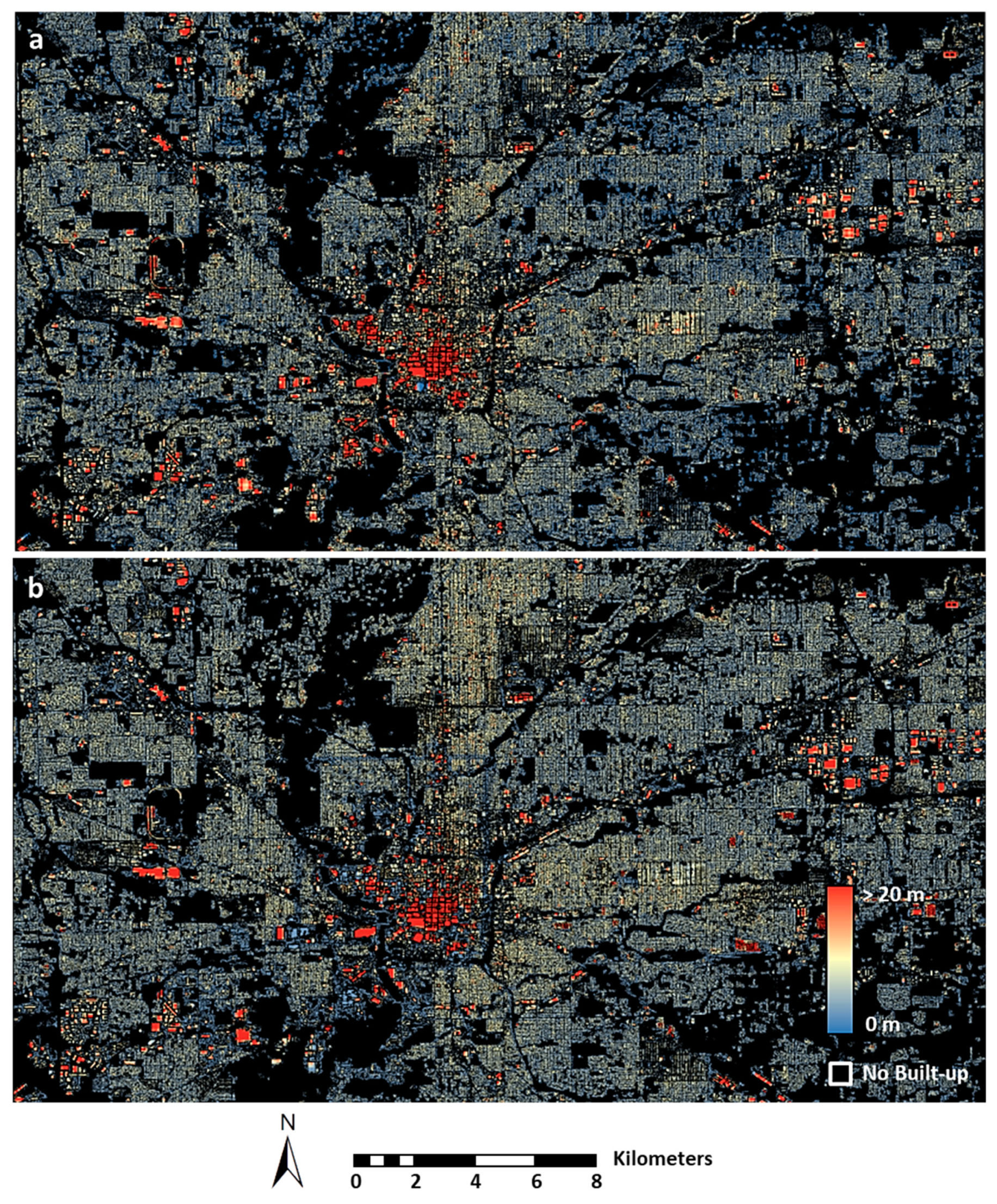
Figure 2 shows the input data, intermediate layers and final result of the GUF-3D processing for the city of Munich, starting with the original TDM-DEM (Figure 2a), then the 12 m nDSM (Figure 2b), the 90 m aggregation of the nDSM (Figure 2c), and the final GUF-3D product indicating the building height estimated for all the building structures (indicated by the BM) at 12 m resolution (Figure 2d). Figure 3 illustrates the GUF-3D layer generated for the reference city Indianapolis (US) in comparison to the 3D information provided by the corresponding ground truth data.
In the following, the results of a first validation campaign for the GUF-3D product are presented for seven cities: Amsterdam (NL), Indianapolis (US), Kigali (RW), Munich (DE), New York (US), Vienna (AT), and Washington (US). The selection of the cities was driven by the availability of accurate reference data on building heights and footprints that had been collected as close in time as possible to the TDX-DEM collection in 2012 (Appendix A). Here it is important to note that the presented work primarily represents a technical feasibility study that aims to indicate the effectiveness and methodological robustness of the described approach to generate urban 3D data at large-scale. A globally more representative and complete validation of the product itself will follow as soon as the GUF-3D data will be available area-wide at a continental or even global scale.
For most cities, the height raster datasets were derived from very high-resolution (VHR) nDSM models, produced based on LiDAR data. On the other hand, building footprints (vector format) were obtained from local cadastral offices (Amsterdam, Munich and Vienna) and the Microsoft building footprints dataset (Indianapolis, New York and Washington) [39]. For the particular case of Kigali, the height data and building footprints were derived from aerial images and VHR Pleiades imagery introduced by Bachofer et al. [40], and this was shared for the study at hand by this group. To produce the final reference 12 m building height layers for each city, the average height was extracted from each VHR height dataset using the corresponding building footprints, which were then rasterized at a 12 m resolution. In total, the area covered by the reference dataset sums up to 3598.6 km2. Generally, it is important to note that for the validation each reference dataset was randomly split into one portion (one-third of the total) used for the empirical determination of thresholds and parameter settings in the context of the system design and parameter tuning, while the remaining two-thirds of the reference data were used for the validation of the final GUF-3D. Therefore, the data was virtually gridded into 500 * 500 pixel cells which were randomly and exclusively assigned in the defined proportions to either the data pool for parameter testing or the one for validation.
When assessing the accuracy of the GUF-3D, two basic components have to be addressed. First, the quality of the extracted building masks (BMs) which is assessed (1) by estimating the accuracy of the identified building pixels in each BM, and (2) by comparing the total building area per city provided by each BM in comparison to the reference data. Secondly, the precision of the estimated heights for the buildings is determined by comparing the height allocated to each BM pixel to its corresponding height in the reference data. Moreover, the dependency between the height estimation errors and the actual heights of the buildings was assessed at the level of building objects.
As detailed in Section 2.2.2, the design of the process for the BM generation provides the flexibility to consider different constellations for the compilation of the final structures, to which the heights formed from the nDSM analysis are assigned. For this research, the BM validation includes the assessment and cross-comparison of the two possible constellations for the building mask: first, the situation that OSM data is available and the BM is thus composed of the components of BMOSM, BMAMP and BMnDSM. Secondly, the BMNoOSM constellation is representative for all regions where no OSM data is available at all, meaning that the final building mask (BM) is solely composed of BMAMP and BMnDSM (here it is important to note that in this version also the ground point detection procedure was run without the consideration of EC1, as defined in Table 1).
The quality and accuracy of the BM and BMNoOSM, respectively, are defined in comparison to the building footprints provided by the reference data. Here, it is important to note that occasionally OSM building polygons also represent the basis for the reference building footprints. Hence, the BM can be expected to be almost identical to the reference mask in these cases or regions. Nonetheless, in those regions lacking any OSM building information, the quality of each BM will solely be defined by the accuracy of the structures provided by BMNoOSM (combination of BMAMP and BMnDSM).
Table 2 presents a summary of the results in the form of a confusion matrix calculated at the pixel level based on the binary building layers (1 = building pixel, 0 = no building pixel) of the BM and the corresponding reference building footprint representations. In terms of building identification, results show that the producer’s accuracy (how well the reference pixels are identified in each BM) ranges between 54.04 and 100% for the BM and between 57.34 and 72.95% for BMNoOSM. The user’s accuracy (the probability of a given building pixel in each BM to be found on the reference) ranges between 53.28% and 88.87% for the BM and between 37.09 and 54.79% for BMNoOSM. Additionally, the overall accuracies of the BM range between 96.78% for Amsterdam and 76.95% for Kigali, whereas the ones for BMNoOSM has values between 82.48% for Indianapolis and 70.28% for New York. Generally, the accuracies are substantially influenced by the proportion of BMNoOSM, with error rates increasing the higher the relative proportion of BMNoOSM to BMOSM is with respect to the BM.
In addition, Figure 4 shows the relative deviation of the BM and BMNoOSM, respectively, in the form of the percentage error between the estimated total building area per city (bar plots) compared to the actual building area derived from the reference data (red lines).
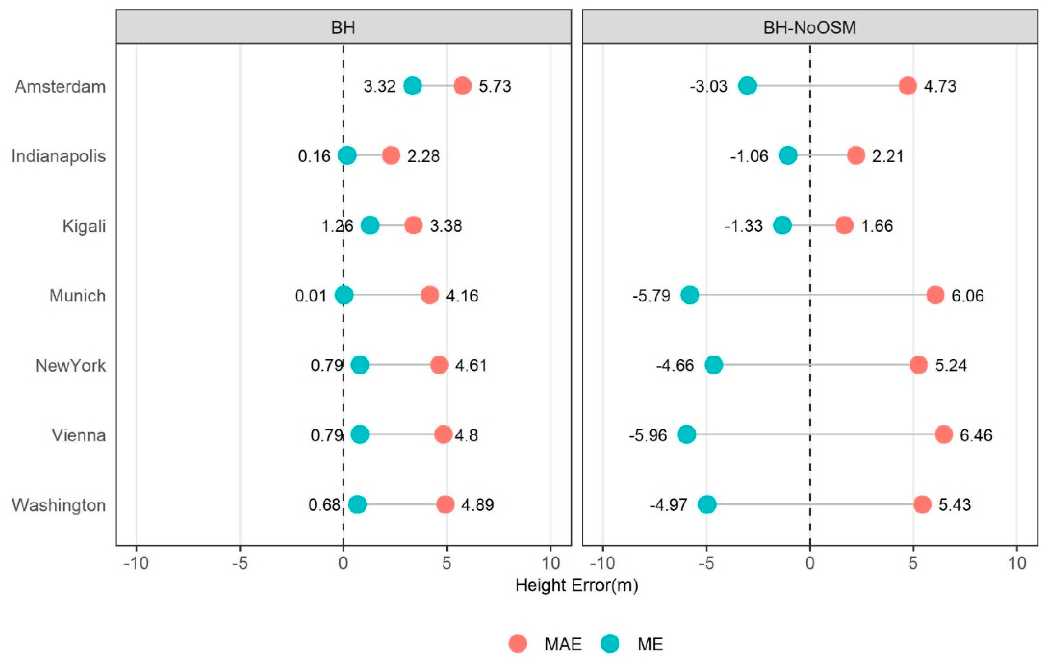
Besides the quality of the building mask, the second key aspect determining the GUF-3D accuracy is the precision of the nDSM modeling and the related height assignment procedure for the identified buildings assigned in the BM and BMNoOSM. The results of a pixel-related accuracy assessment based on the comparison between the estimated building heights (BH and BHNoOSM) and the corresponding values given by the reference data for all the studied cities are illustrated in Figure 5. In terms of the BH (heights estimated for building structures given by the BM), the results show that the mean error (ME) between the estimated heights and the real heights ranges from 0.01 m for Munich to 3.32 m for Amsterdam, indicating a tendency towards a systematic overestimation of the height values at the pixel level. Accordingly, the ME values range from −1.06 m for Indianapolis to −5.96 m for Vienna, based on BHNoOSM. Here, however, results show a systematic underestimation of the height values. The reason for this underestimation is the considerable overestimation of the real building area already reported in the context of the BM validation. This leads to a disaggregation of the collected 12 m heights aggregated at the 90 m cell into too many building pixels. Consequently, the assigned heights are (proportionally at the 12 m level) too low.
In addition to the ME, the mean absolute error (MAE) was calculated in order to develop a better understanding of the local distribution and range of height estimation errors. On the one hand, the BH reports its lowest MAE value of 2.28 m for Indianapolis and its highest MAE value of 4.89 m for Washington. On the other hand, BHNoOSM reports its lowest MAE value of 2.21 m Indianapolis and its highest MAE value of 6.46 m for Vienna.
While Table 2, Figure 4 and Figure 5 present the accuracy results of the GUF-3D in terms of two different components, namely the quality of the BM and the local height estimation BH at the pixel level, a complete interpretation of the results has to be derived simultaneously from both assessments. Due to the incorporation of BMOSM, which is comparable to many of the reference building footprints (see results in Table 2), the reported percentage errors in terms of the building area are lower for the BM in comparison to BMNoOSM (see Figure 4). These lower percentage errors translate into overall more accurate building heights (lower ME and MAE values of the BH), as the final 12 m height values are more accurate due to the lower values for the percentage built-up coverage (BCA). Accordingly, with the large building area overestimations reported for BMNoOSM, the ME and MAE values reported by BHNoOSM are larger as well, due to the influence of higher BCA values in the final 12 m height values. Here, for cities such as Indianapolis and Kigali, where the BMNoOSM presented the lower overestimations of the building area, the ME and MAE values are also lower in comparison to the rest of the countries, which confirms the correlation between both components.
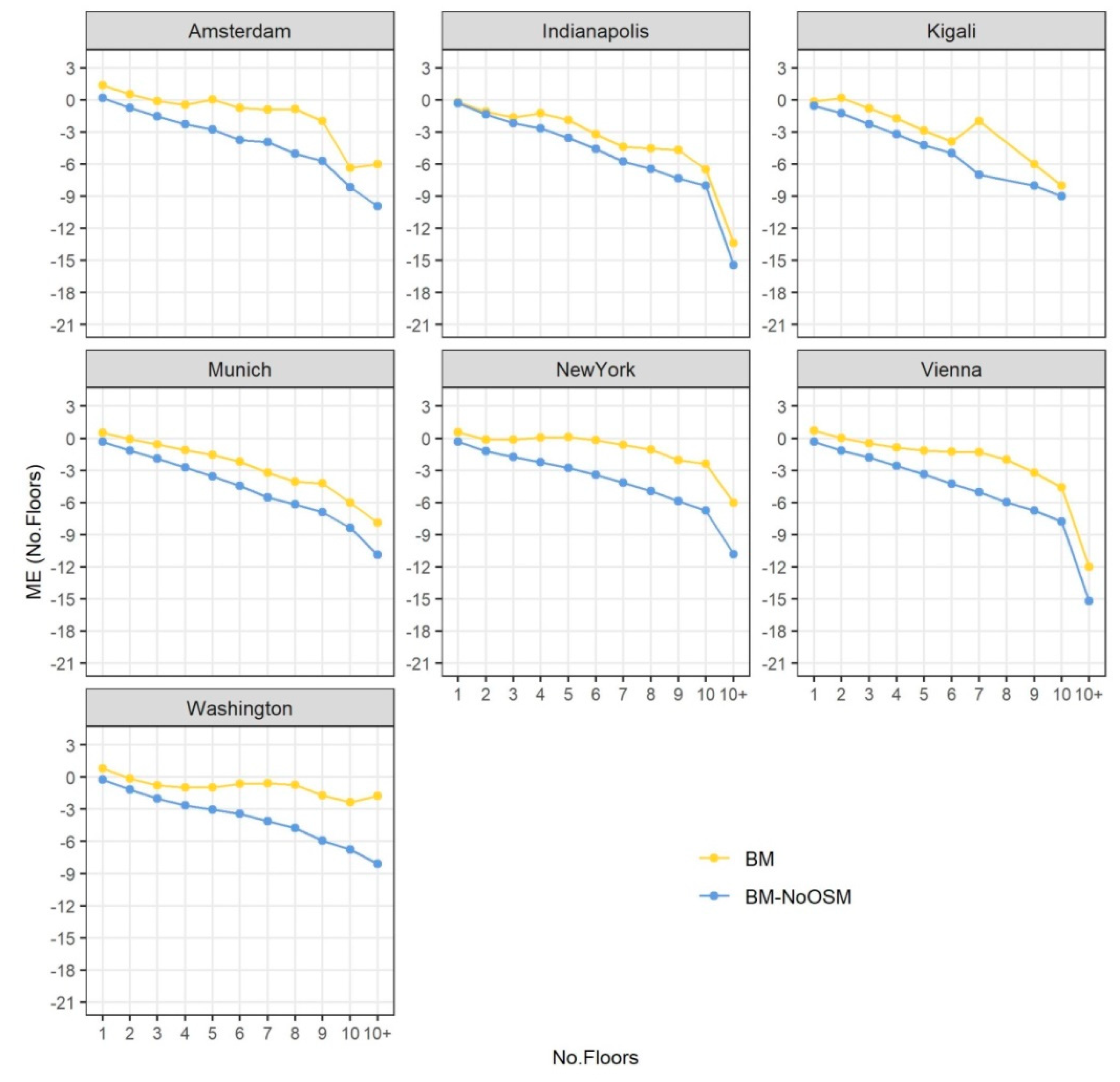
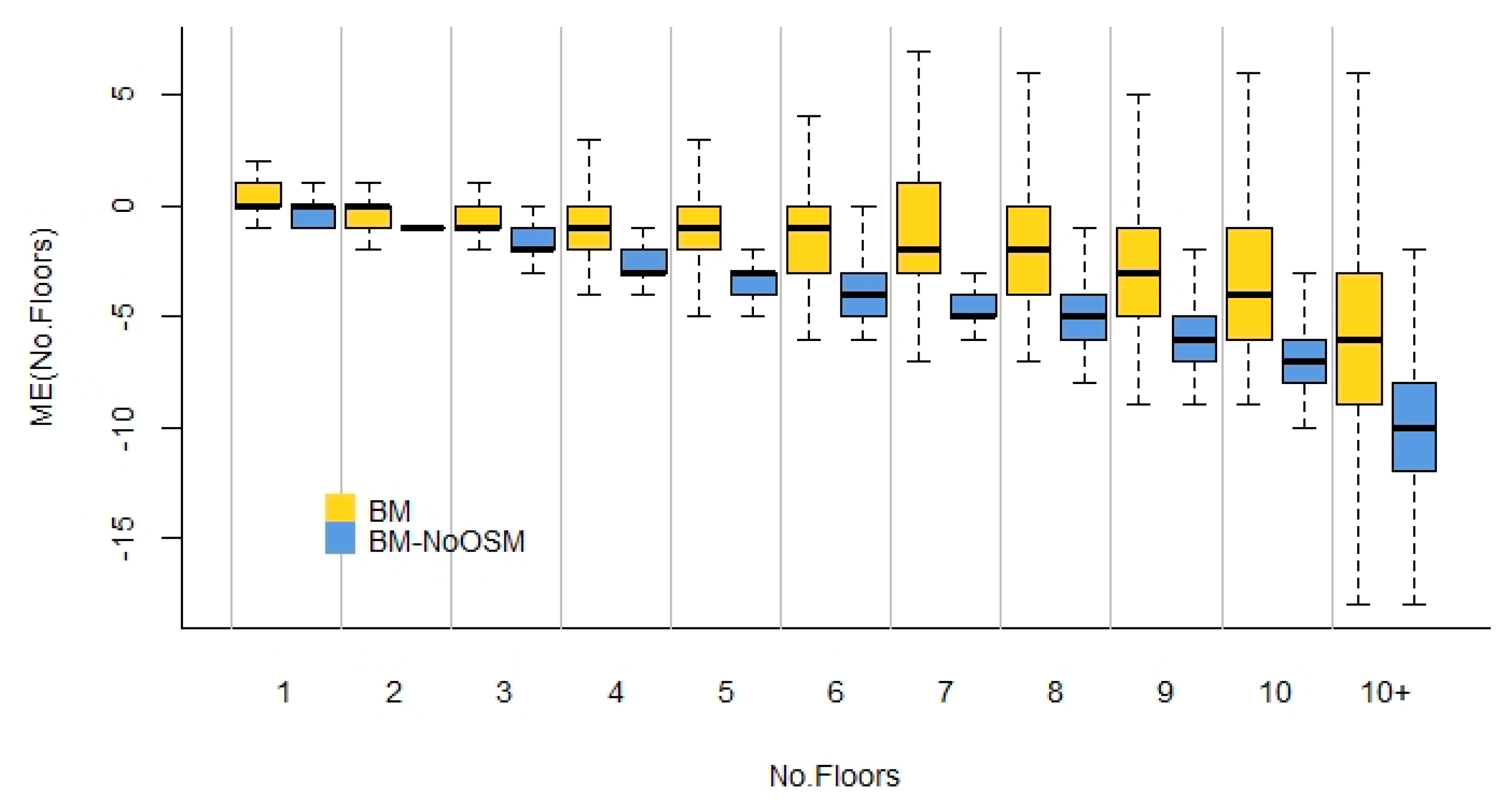
An additional analysis was carried out to investigate the dependency between the actual height of the buildings and the amount of estimation errors at the building level. Here, the average height of each reference building footprint was extracted from the reference data and each BM of the GUF-3D. The average height was then converted into the number of floors, considering a standard height of 3 m for a typical floor. From here, the mean error ME was calculated between the estimated number of floors derived by the two BM versions and the reference data. Figure 6 shows the ME values reported by each BM according to the number of floors for each study city.
Results indicate a systematic increase of error, with higher underestimation errors from the low- to high-rise buildings. This behavior can mainly be attributed to the layover effect, where the actual pixels belonging to high buildings are mapped closer to the satellites footprint and therewith positioned outside the actual location of the building footprint. In other words, as the height of the building increases, the average height of the building footprints is calculated on the basis of the backscatter coming from the lower parts of the building, leading to increasing errors of underestimations with increasing building heights. At the same time, the accurate representation of building footprints and forms might be limited due to the additional SAR-specific effects such as multiple scattering or shadowing.
Finally, in order to better assess the effectiveness of each BM, the distribution of the ME was aggregated over all the studied cities as shown in Figure 7. The results indicate that the ME values derived from the BH are slightly lower than those reported by BHNoOSM. Here, the interquartile range, namely between the 25% and 75% quartiles, and the ME values are reported by the BH range from minus two to one floor(s) for buildings between one and five floors in height, minus six to one floor(s) for buildings between six and ten floors height, and minus eighteen to minus three floors for buildings higher than ten floors. Here, however, it is worth noting that from the 2,077,215 reference buildings considered for this study, 99.37% are buildings with a height between one and five floors, 0.5% are buildings with six to ten floors, and only 0.13% are buildings higher than 10 floors. Hence, the largest errors of underestimation are only present for a very small number of buildings.

4. Discussion

Considering the analyses and (relative) comparisons at the city level, the obtained results suggest the ability of the developed approach to provide accurate information on the absolute and relative differences in the urban morphology. Focusing on scenarios where OSM data is available, the reported mean error (ME) in comparison to the reference data ranges between 0.01 m and 3.32 m at the city level. The local absolute errors lie between 2.28 m and 5.73 m. The GUF-3D error statistics also indicate a basic suitability of the product to examine the 3D urban properties at the level of individual buildings, with mean errors ranging between minus two and one floor(s) for buildings up to five stories high. Moreover, the results reveal the increasing deviations between the estimated and true building heights from the low- to high-rise buildings.
In general, the analyses have shown that the representation of the detailed 3D building pattern and related morphological structuring significantly profits from the availability of building outlines provided by OSM. If only the 12 m BMAMP and BMnDSM data are available (BMNoOSM scenario), the ability to accurately delineate individual buildings is limited. Notably, the typical side-by-side arrangement of small single houses with surrounding trees or hedges in residential areas frequently leads to an entire (virtual) row of houses and interlaced trees being delineated as one elongated building structure. Due to the typical small-scale dimension of the vegetation features, the NDVI-based vegetation masking cannot help to avoid this effect. However, the related errors and ambiguities have been quantified by the reported systematic average overestimation of the building footprints (Figure 4) in case of a total lack of OSM building data. As an approach to (numerically) correct this effect, the built-up coverage area (Equation (12)) and area adaptation factor ( f A ) (Equation (9)) were introduced for the optimized estimation of the building heights (BHs) and the building volumes (BVs).
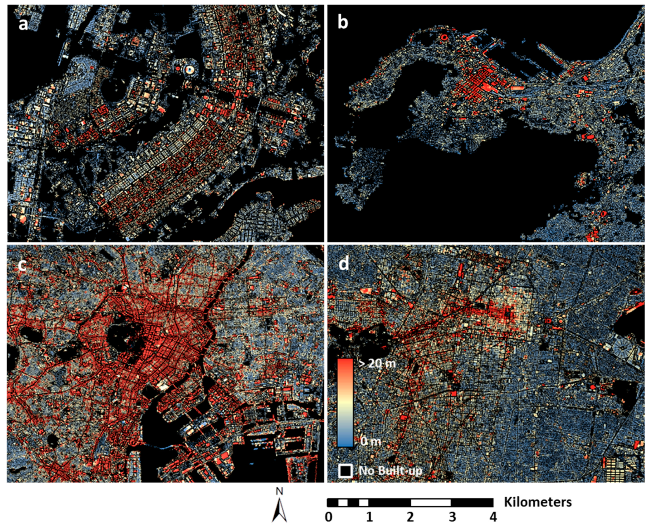
Apart from the presented numerical validation based on ground truth information, the GUF-3D was generated for >100 additional cities and settlement areas distributed all over the world in order to provide complementary qualitative insights into the types and distribution of errors in a varying environmental context (e.g., urban structural, architectural cultural settings, topography, geomorphology, climate, etc.). Figure 8 illustrates various examples of these additional GUF-3D products, including the cities of Brasilia (BR), Cape Town (ZA), Tokyo (JP), and Mexico City (MX).
Thereby, the positive observations reported in the context of the quantitative validation campaign (see Section 3) could generally be confirmed. However, the related visual inspections also showed—though locally limited—difficulties of the presented approach to accurately estimate the building height in certain very high-density urban areas (e.g., informal settlements, old city cores with high buildings and very narrow streets) where, under the intrinsic constraints of the SAR-related side-looking geometry, a spatially consistent visibility of the ground surface (e.g., radar shadow) is not given. Moreover, the quality of the TDX-DEM itself is occasionally poor in these areas as well due to phase ambiguities resulting from multiple scattering, and the under sampling of the 12 m radar intensity images with respect to the small-scale urban structures. Consequently, the height of the built-up structures in these regions is underestimated because of a significant amount of estimated ground points being falsely positioned on building structures that show a lower height compared to their neighbors.
Inaccuracies could also be observed in built environments with very extreme topographic situations (e.g., almost continuous building coverage in very rugged terrain). Here, the achievable density and distribution of ground points is sometimes, even under optimal performances, too low to allow for a complete and accurate representation of the local peaks or sinks in the terrain. As a result, these topographic structures—and the buildings on top of them—are virtually cut by the terrain interpolation procedure. Consequently, the buildings in the direct vicinity suffer from false height assignments in the form of a drastic overestimation, in the case of terrain peaks that were cut, or severe underestimations for houses in sinks that were virtually filled. A few difficulties were also discovered in the case of large urban quarters entirely consisting of extremely high buildings, where the top of the buildings is shifted by multiple pixels so that their according height value might even lie outside the aggregated 90 m cells. Finally, in rural settlements with predominating one-story houses, the determined heights of buildings are sometimes overestimated locally due to the influence of single or small groups of high trees that push the local nDSM heights upwards, but cannot be eliminated by the vegetation mask due to a lack of spectral significance and clarity (mixed pixels) which would allow a clear separation from the surrounding built-up structures in the NDVI layer.
Generally, a test-wise application of the method to a large variety of heterogeneous city and settlement types located all over the globe showed that the key information which is analyzed— namely, the characteristics of the local height variations in the TDX-DEM—is a rather robust and stable feature all around the world. Nevertheless, in an upcoming comprehensive validation campaign, all the uncertainties of the proposed methodology will be systematically identified and quantitatively and qualitatively analyzed in order to define the technical improvements of the approach if required. This campaign will also be used to underpin and supplement the representativeness and statistical significance of the statistical findings presented in this study (e.g., an extended and more balanced coverage of reference sites for all the key urban and rural settlement types in the major cultural/geographic zones on Earth).

5. Conclusions and Outlook

In this paper, the Global Urban Footprint 3D (GUF-3D) processing framework was introduced and validated for seven city regions. This modular workflow includes the rule-based analysis of TanDEM-X digital elevation (TDX-DEM) and radar amplitude data (TDX-AMP) in combination with auxiliary layers such as building outlines derived from Open Street Map (OSM), a vegetation mask generated based on Sentinel-2 imagery, and a global map of human settlements defined by the Global Urban Footprint (GUF). The resulting GUF-3D product defines the relative local heights of all building structures within a settlement at 12 m spatial resolution.
The outcomes of a first validation campaign based on the absolute reference data collected for seven globally distributed cities indicate a high potential of the new method to effectively map the vertical extent of the built-up structures within human settlements. This observation is confirmed by an additional 100 (and more) spots located on all the continents and covering the most important urban types for which the GUF-3D was generated as well. The related qualitative inspections show that the typical characteristics of local height variations in the built environment represent a geographically stable and distinct feature which can effectively be analyzed based on the 12 m TDX-DEM. However, whereas the approach allows for an efficient description of the urban morphology at city level, the potential related to a precise height estimation for individual buildings is still limited, especially in the case of a lack of precise information on the buildings outlines (e.g., such as provided by OSM). In this context, the study documented the local variations of height estimation errors for specific complex settings such as very high buildings (underestimation of building heights), small one-story houses surrounded by significantly higher vegetation (overestimation of building heights), very high-density urban areas with quite narrow streets and/or no open (ground) space in between (underestimation of building height), or settlements built on very rugged terrain (over- and underestimation of building heights). Nevertheless, the general dimension and effects of these limitations have been reported and quantified in the Results section and are comprehensively discussed in the Discussion section.
To conclude, the presented method is supposed to pave the way for the generation of large-scale GUF-3D datasets that can be expected to considerably push studies related to refined large-scale analyses of the vertical built-up extent, built-up densities, urban morphological properties, and volumetric characteristics (e.g., floor space index). These parameters are key inputs to improve the modeling of population distributions, urban climates and carbon emissions, economic variables, or vulnerabilities and risks. In the context of the Corona/Covid-19 pandemic, the GUF-3D technique has recently been used in combination with the WSF 2015 settlement mask [12] by the World Bank [41] to predict contagion risk hotspots in several African, Asian and South American cities.
Once more, GUF-3D datasets have been processed and validated, and an open and free provision is foreseen, for instance via German Aerospace Center’s (DLR) Earth Observation Center (EOC) Geoservice (https://geoservice.dlr.de) and the Urban Thematic Exploitation Platform [42] (https://urban-tep.eu).

Author Contributions

Conceptualization, T.E.; methodology, T.E., J.Z., M.M. (Mattia Marconcini) and B.L.; software, J.Z. and T.E.; validation, D.P.-L., M.M. (Milena Mönks) and E.B.; formal analysis, A.R.; investigation, A.R. and F.B.; resources, T.E. and S.L.; data curation, D.P.-L., J.Z., E.B. and A.M.-M.; writing—original draft preparation, T.E., D.P.-L. and J.Z.; writing—review and editing, M.M. (Mattia Marconcini), A.R., F.B., M.M. (Milena Mönks) and B.L.; visualization, T.E. and D.P.-L.; supervision, S.D.; funding acquisition, T.E., S.D. and S.L. All authors have read and agreed to the published version of the manuscript.

Funding

The methodological research was funded based on the internal funding of the German Aerospace Center (DLR) and by the European Space Agency (ESA) in the context of the project “Artificial Intelligence for Smart Cities (AI4SC)”, ESA contract no. 4000126100/19/I-EF. The validation and application development were co-financed by the EU-funded ACP-EU Natural Disaster Risk Reduction Program, managed by the Global Facility for Disaster Reduction and Recovery (World Bank, project “Satellite Monitoring Service of Urbanization in Africa”, contract no. 7194331). Moreover, parts of the validation were conducted in the context of the project “Development of a concept for information retrieval about the building stock in Germany with remote sensing”, funded by the German Federal Institute for Research on Building, Urban Affairs and Spatial Development within the Federal Office for Building and Regional Planning (reference number 10.08.17.7-18.13).

Acknowledgments

The authors would like to thank the TerraSAR-X Science Team for providing the global SAR data used to derive the GUF layer. We also thank the World Bank (Caroline Gevaert, Edward Charles Anderson, Vivien Deparday, Walker Kosmidou-Bradley) for their substantial support of the validation campaign.

Conflicts of Interest

The authors declare no conflict of interest.

Appendix A

The following table provides information about the sources of the reference data used for the validation campaign.
CitySourceData TypeAcquisition
Amsterdam, NLhttps://ahn.arcgisonline.nl/ahnviewer/DSM, DEM2012
https://zakelijk.kadaster.nl/bagBuilding Footprints
Indianapolis, UShttp://opentopo.sdsc.edu/datasetMetadata?otCollectionID=OT.062012.4326.1LiDAR point cloud2010–2012
Kigali, RWhttps://zenodo.org/record/3239271#.Xr0IDsBS-UkPleiades Satellite Image2015
Munich, DEGeoBasis-DE/BKG [2020]: https://gdz.bkg.bund.de/index.php/default/digitale-geodaten/sonstige-geodaten/3d-gebaudemodelle-lod1-deutschland-lod1-de.html3D Building Model (LoD1-DE); CityGML version 1.0.0, encoding standard 08-007r12013–2018
New York, UShttps://coast.noaa.gov/htdata/lidar1_z/geoid12b/data/4920/LiDAR point cloud2014
Vienna, AThttps://www.wien.gv.at/ma41datenviewer/public/LOD1 Building Footprints2007
DSM, DEM2010–2018
Washington, UShttps://dc-lidar-2015.s3.amazonaws.com/index.htmlLiDAR point cloud2015

References

  1. United Nations Department of Economic and Social Affairs Population Division. World Population Prospects: The Highlights. 2019. Available online: https://population.un.org/wpp/Publications/Files/WPP2019_Highlights.pdf (accessed on 24 June 2020).
  2. United Nations Development Programme. Sustainable Urbanization Strategy: UNDP’s Support to Sustainable, Inclusive and Resilient Cities in Developing World; United Nations: New York, NY, USA, 2016; Available online: http://www.undp.org/content/dam/undp/library/Sustainable%20Development/Urbanization/UNDP_Urban-Strategy.pdf (accessed on 24 June 2020).
  3. d’Amour, C.B.; Reitsma, F.; Baiocchi, G.; Barthel, S.; Güneralp, B.; Erb, K.-H.; Haberl, H.; Creutzig, F.; Seto, K.C. Future urban land expansion and implications for global croplands. Proc. Natl. Acad. Sci. USA 2017, 114, 8939–8944. [Google Scholar] [CrossRef] [PubMed] [Green Version]
  4. Global Power Synergy Public Company. Sustainability Report Chatuchak, Bangkok, 2019. Available online: https://www.gpscgroup.com/Uploads/elFinder/sustaibability/sustainability_reporting/20190325-gpsc-sd2018-en.pdf (accessed on 24 June 2020).
  5. Lützkendorf, T.; Balouktsi, M. Assessing a sustainable urban development: Typology of indicators and sources of information. Proced. Environ. Sci. 2017, 38, 546–553. [Google Scholar] [CrossRef]
  6. Mahendra, A.; Seto, K.C. Upward and Outward Growth: Managing Urban Expansion for More Equitable Cities in the Global South; World Resources Report: Washington, DC, USA, 2019. [Google Scholar]
  7. Esch, T.; Marconcini, M.; Felbier, A.; Roth, A.; Heldens, W.; Huber, M.; Schwinger, M.; Taubenböck, H.; Müller, A.; Dech, S. Urban footprint processor—Fully automated processing chain generating settlement masks from global data of the TanDEM-X mission. IEEE Geosci. Remote Sens. Lett. 2013, 10, 1617–1621. [Google Scholar] [CrossRef] [Green Version]
  8. Pesaresi, M.; Ehrlich, D.; Ferri, S.; Florczyk, A.; Freire, S.; Halkia, M.; Julea, A.; Kemper, T.; Soille, P.; Syrris, V. Operating Procedure for the Production of the Global Human Settlement Layer from Landsat Data of the Epochs 1975, 1990, 2000 and 2014; Publications Office of the European Union: Brussels, Belgium, 2016; pp. 1–62. [Google Scholar] [CrossRef]
  9. Tiecke, T.G.; Liu, X.; Zhang, A.; Gros, A.; Li, N.; Yetman, G.; Kilic, T.; Murray, S.; Blankespoor, B.; Prydz, E.B.; et al. Mapping the world population one building at a time. arXiv 2020, arXiv:1712.05839. [Google Scholar]
  10. Román, M.O.; Wang, Z.; Sun, Q.; Kalb, V.; Miller, S.D.; Molthan, A.; Schultz, L.; Bell, J.; Stokes, E.C.; Pandey, B. NASA’s Black Marble nighttime lights product suite. Remote Sens. Environ. 2018, 210, 113–143. [Google Scholar] [CrossRef]
  11. Florczyk, A.J.; Melchiorri, M.; Zeidler, J.; Corbane, C.; Schiavina, M.; Freire, S.; Sabo, F.; Politis, P.; Esch, T.; Pesaresi, M. The Generalised Settlement Area: Mapping the Earth surface in the vicinity of built-up areas. Int. J. Digit. Earth 2020, 13, 45–60. [Google Scholar] [CrossRef]
  12. Marconcini, M.; Metz-Marconcini, A.; Üreyen, S.; Palacios-Lopez, D.; Hanke, W.; Bachofer, F.; Zeidler, J.; Esch, T.; Gorelick, N.; Kakarla, A. Outlining where humans live—The World Settlement Footprint 2015. arXiv 2019, arXiv:1910.12707. [Google Scholar]
  13. Brown De Colstoun, E.C.; Huang, C.; Wang, P.; Tilton, J.C.; Tan, B.; Phillips, J.; Niemczura, S.; Ling, P.-Y.; Wolfe, R. Documentation for the Global Man-Made Impervious Surface (GMIS) Dataset from Landsat. NASA Socioecon. Data Appl. Cent. Palisade 2017. [Google Scholar] [CrossRef]
  14. Esch, T.; Bachofer, F.; Heldens, W.; Hirner, A.; Marconcini, M.; Palacios-Lopez, D.; Roth, A.; Üreyen, S.; Zeidler, J.; Dech, S. Where we live—A summary of the achievements and planned evolution of the global urban footprint. Remote Sens. 2018, 10, 895. [Google Scholar] [CrossRef] [Green Version]
  15. Palacios-Lopez, D.; Bachofer, F.; Esch, T.; Heldens, W.; Hirner, A.; Marconcini, M.; Sorichetta, A.; Zeidler, J.; Kuenzer, C.; Dech, S.; et al. New Perspectives for Mapping Global Population Distribution Using World Settlement Footprint Products. Sustainability 2019, 11, 6056. [Google Scholar] [CrossRef] [Green Version]
  16. Lloyd, C.T.; Chamberlain, H.; Kerr, D.; Yetman, G.; Pistolesi, L.; Stevens, F.R.; Gaughan, A.E.; Nieves, J.J.; Hornby, G.; MacManus, K. Global spatio-temporally harmonised datasets for producing high-resolution gridded population distribution datasets. Big Earth Data 2019, 3, 108–139. [Google Scholar] [CrossRef] [PubMed] [Green Version]
  17. Lafarge, F.; Descombes, X.; Zerubia, J.; Pierrot-Deseilligny, M. Structural approach for building reconstruction from a single DSM. IEEE Trans. Pattern Anal. Mach. Intell. 2008, 32, 135–147. [Google Scholar] [CrossRef] [PubMed] [Green Version]
  18. Qin, J.; Fang, C.; Wang, Y.; Li, G.; Wang, S. Evaluation of three-dimensional urban expansion: A case study of Yangzhou City, Jiangsu Province, China. Chin. Geogr. Sci. 2015, 25, 224–236. [Google Scholar] [CrossRef]
  19. Zhang, W.; Li, W.; Zhang, C.; Ouimet, W.B. Detecting horizontal and vertical urban growth from medium resolution imagery and its relationships with major socioeconomic factors. Int. J. Remote Sens. 2017, 38, 3704–3734. [Google Scholar] [CrossRef]
  20. Zambon, I.; Colantoni, A.; Salvati, L. Horizontal vs vertical growth: Understanding latent patterns of urban expansion in large metropolitan regions. Sci. Total Environ. 2019, 654, 778–785. [Google Scholar] [CrossRef]
  21. Xu, G.; Dong, T.; Cobbinah, P.B.; Jiao, L.; Sumari, N.S.; Chai, B.; Liu, Y. Urban expansion and form changes across African cities with a global outlook: Spatiotemporal analysis of urban land densities. J. Clean. Prod. 2019, 224, 802–810. [Google Scholar] [CrossRef]
  22. Shahzad, M.; Zhu, X.X. Detection of buildings in spaceborne tomosar point clouds via hybrid region growing and energy minimization technique. Urb. Remote Sens. Event (JURSE) 2015, 1–4. [Google Scholar] [CrossRef] [Green Version]
  23. Frolking, S.; Milliman, T.; Seto, K.C.; Friedl, M.A. A global fingerprint of macro-scale changes in urban structure from 1999 to 2009. Environ. Res. Lett. 2013, 8, 024004. [Google Scholar] [CrossRef]
  24. Mathews, A.J.; Frazier, A.E.; Nghiem, S.V.; Neumann, G.; Zhao, Y. Satellite scatterometer estimation of urban built-up volume: Validation with airborne lidar data. Int. J. Appl. Earth Obs. 2019, 77, 100–107. [Google Scholar] [CrossRef]
  25. Marconcini, M.; Marmanis, D.; Esch, T.; Felbier, A. A novel method for building height estmation using TanDEM-X data. IEEE Geosci. Remote Sens. Symp. 2014, 4804–4807. [Google Scholar]
  26. Clinton, N.; Stuhlmacher, M.; Miles, A.; Uludere Aragon, N.; Wagner, M.; Georgescu, M.; Herwig, C.; Gong, P. A global geospatial ecosystem services estimate of urban agriculture. Earth’s Future 2018, 6, 40–60. [Google Scholar] [CrossRef]
  27. Geiß, C.; Leichtle, T.; Wurm, M.; Pelizari, P.A.; Standfuß, I.; Zhu, X.X.; So, E.; Siedentop, S.; Esch, T.; Taubenböck, H. Large-area characterization of urban morphology—Mapping of built-up height and density using TanDEM-X and Sentinel-2 data. IEEE J. Sel. Top. Appl. Earth Obs. Remote Sens. 2019, 12, 2912–2927. [Google Scholar] [CrossRef]
  28. Li, M.; Koks, E.; Taubenböck, H.; van Vliet, J. Continental-scale mapping and analysis of 3D building structure. Remote Sens. Environ. 2020, 245, 111859. [Google Scholar] [CrossRef]
  29. Esch, T.; Heldens, W.; Hirner, A.; Keil, M.; Marconcini, M.; Roth, A.; Zeidler, J.; Dech, S.; Strano, E. Breaking new ground in mapping human settlements from space—The Global Urban Footprint. ISPRS J. Photogramm. Remote Sens. 2017, 134, 30–42. [Google Scholar] [CrossRef] [Green Version]
  30. Esch, T.; Üreyen, S.; Zeidler, J.; Metz-Marconcini, A.; Hirner, A.; Asamer, H.; Tum, M.; Böttcher, M.; Kuchar, S.; Svaton, V. Exploiting big earth data from space—First experiences with the timescan processing chain. Big Earth Data 2018, 2, 36–55. [Google Scholar] [CrossRef] [Green Version]
  31. Zink, M.; Bachmann, M.; Brautigam, B.; Fritz, T.; Hajnsek, I.; Moreira, A.; Wessel, B.; Krieger, G. TanDEM-X: The new global DEM takes shape. IEEE Trans. Geosci. Remote Sens. 2014, 2, 8–23. [Google Scholar] [CrossRef]
  32. Wessel, B.; Huber, M.; Wohlfart, C.; Marschalk, U.; Kosmann, D.; Roth, A. Accuracy assessment of the global TanDEM-X Digital Elevation Model with GPS data. ISPRS J. Photogramm. Remote Sens. 2018, 139, 171–182. [Google Scholar] [CrossRef]
  33. Open Street Map Contributors. Available online: https://www.openstreetmap.org (accessed on 24 June 2020).
  34. Wendleder, A.; Wessel, B.; Roth, A.; Breunig, M.; Martin, K.; Wagenbrenner, S. TanDEM-X water indication mask: Generation and first evaluation results. IEEE J. Sel. Top. Appl. Earth Obs. Remote Sens. 2012, 6, 171–179. [Google Scholar] [CrossRef] [Green Version]
  35. Gorelick, N.; Hancher, M.; Dixon, M.; Ilyushchenko, S.; Thau, D.; Moore, R. Google Earth Engine: Planetary-scale geospatial analysis for everyone. Remote Sens. Environ. 2017, 202, 18–27. [Google Scholar] [CrossRef]
  36. De Reu, J.; Bourgeois, J.; Bats, M.; Zwertvaegher, A.; Gelorini, V.; De Smedt, P.; Chu, W.; Antrop, M.; De Maeyer, P.; Finke, P. Application of the topographic position index to heterogeneous landscapes. Geomorphology 2013, 186, 39–49. [Google Scholar] [CrossRef]
  37. Esch, T.; Schenk, A.; Ullmann, T.; Thiel, M.; Roth, A.; Dech, S. Characterization of land cover types in TerraSAR-X images by combined analysis of speckle statistics and intensity information. IEEE Trans. Geosci. Remote Sens. 2011, 49, 1911–1925. [Google Scholar] [CrossRef]
  38. GDAL/OGR Contributors. GDAL/OGR Geospatial Data Abstraction Software Library. Available online: https://gdal.org (accessed on 24 June 2020).
  39. Heris, M.P.; Foks, N.; Bagstad, K.; Troy, A. A National Dataset of Rasterized Building Footprints for the U.S.; U.S. Geological Survey Data Release: Sunrise Valley Drive Reston, VA, USA, 2020. [Google Scholar] [CrossRef]
  40. Bachofer, F.; Braun, A.; Adamietz, F.; Murray, S.; d’Angelo, P.; Kyazze, E.; Mumuhire, A.P.; Bower, J. Building stock and building typology of Kigali, Rwanda. Data 2019, 4, 105. [Google Scholar] [CrossRef] [Green Version]
  41. Bhardwaj, G.; Esch, T.; Lall, S.V.; Marconcini, M.; Soppelsa, M.E.; Wahba, S. Cities, Crowding, and the Coronavirus: Predicting Contagion Risk Hotspots. Available online: https://blogs.worldbank.org/sustainablecities/cities-crowding-and-coronavirus-predicting-contagion-risk-hotspots (accessed on 24 June 2020).
  42. Esch, T.; Asamer, H.; Bachofer, F.; Balhar, J.; Böttcher, M.; Boissier, E.; D’Angelo, P.; Gevaert, C.; Hirner, A.; Jupova, K.; et al. Digital World meets Urban Planet—New Prospects for Evidence-based Urban Studies Arising from Joint Exploitation of Big Earth Data, Information Technology and Shared Knowledge. Int. J. Digit. Earth 2018, 13, 136–157. [Google Scholar] [CrossRef]
Figure 1. Schematic view of the Global Urban Footprint 3D (GUF-3D) production workflow.
Remotesensing 12 02391 g001
Figure 2. TanDEM-X digital elevation model (a) at 12 m resolution, the normalized digital elevation model (nDSM) derived from the TanDEM-X data (b), the nDSM aggregated to 90 m, with vertical vegetation components removed (c), and the final GUF-3D product (d).
Remotesensing 12 02391 g002
Figure 3. The GUF-3D layer generated for Indianapolis (a) in comparison to the reference data available for this region (b).
Remotesensing 12 02391 g003
Figure 4. Percentage error per city between the estimated and actual total building area.
Remotesensing 12 02391 g004
Figure 5. Mean error (ME) and mean absolute error (MAE) of building height (BH) estimation achieved for the seven study cities, given for the two cases of existing Open Street Map (OSM) data and a processing without OSM integration (BHNoOSM).
Remotesensing 12 02391 g005
Figure 6. Mean error (ME) reported in the number of floors by each building mask (BM) for each study city.
Remotesensing 12 02391 g006
Figure 7. Mean error (ME) reported in the number of floors by each BM for all the studied cities.
Remotesensing 12 02391 g007
Figure 8. Examples of the GUF-3D layer derived for several globally distributed city regions such as Brasilia (a), Cape Town (b), Tokyo (c), and Mexico City (d).
Remotesensing 12 02391 g008
Table 1. Rules to identify ground points based on a set of exclusion (EC) and inclusion criteria (IC).
CriterionRule
EC1sLOSM = 1
EC2pLDEM1 < 0.1
EC3sLAMP = 1 AND pLDEM1 ≥ −1.5
EC4sLOSM-AMP ≥ 0.6 AND ((pLDEM2 ≥ 0.8 AND pLDEM3 ≥ 0.96) OR pLDEM4 ≥ 1.0 OR pLDEM3 ≥ 1.0)
IC1pLDEM3 ≥ 0.93
IC2pLDEM3 ≥ 0.96 AND pLDEM1 < −5.0
IC3pLDEM4 ≥ 0.96
Table 2. Overall accuracy (OA), producer’s accuracy (PA) and user’s accuracy (UA) of the building masks (BMs) generated for the test areas.
CityBMBMNoOSM
OA [%]PA [%]UA [%]OA [%]PA [%]UA [%]
Amsterdam96.7810083.6081.3872.9545.74
Indianapolis84.1258.1659.9282.4862.4154.79
Kigali76.9554.0153.2875.5357.3450.39
Munich95.4310078.2275.9072.5337.09
New York96.3010088.8770.2871.3749.80
Vienna96.4910082.5478.8272.4641.98
Washington96.6010086.1675.9670.3245.62

