Convective Initiation Proxies for Nowcasting Precipitation Severity Using the MSG-SEVIRI Rapid Scan

 ,
,  ,
,  , ,
, ,  ,
,  , , and
Abstract
:1. Introduction
2. Materials and Methods
2.1. Dataset Collection Criteria
2.2. Static Approach
3. Results and Discussion
4. Conclusions
Author Contributions
Funding
Conflicts of Interest
References
- Wang, Y.; Coning, E.; Harou, A.; Jacobs, W.; Joe, P.; Nikitina, L.; Roberts, R.; Wang, J.; Wilson, J.; Atencia, A.; et al. Guidelines for Nowcasting Techniques; WMO-No. 11988; World Meteorological Organization: Geneva, Switzerland, 2017; ISBN 978-92-63-11198-2. Available online: https://library.wmo.int/doc_num.php?explnum_id=3795 (accessed on 8 August 2020).
- Mecikalski, J.R.; Bedka, K.M. Forecasting Convective Initiation by Monitoring the Evolution of Moving Cumulus in Daytime GOES Imagery. Mon. Weather Rev. 2006, 134, 49–78. [Google Scholar] [CrossRef] [Green Version]
- Bedka, K.; Brunner, J.; Dworak, R.; Feltz, W.; Otkin, J.; Greenwald, T. Objective Satellite-Based Detection of Overshooting Tops Using Infrared Window Channel Brightness Temperature Gradients. J. Appl. Meteorol. Climatol. 2010, 49, 181–202. [Google Scholar] [CrossRef]
- Sieglaff, J.M.; Hartung, D.C.; Feltz, W.F.; Cronce, L.M.; Lakshmanan, V. A Satellite-Based Convective Cloud Object Tracking and Multipurpose Data Fusion Tool with Application to Developing Convection. J. Atmos. Ocean. Technol. 2013, 30, 510–525. [Google Scholar] [CrossRef]
- Cintineo, J.L.; Pavolonis, M.J.; Sieglaff, J.M.; Lindsey, D.T. An Empirical Model for Assessing the Severe Weather Potential of Developing Convection. Weather Forecast. 2014, 29, 639–653. [Google Scholar] [CrossRef] [Green Version]
- Bedka, K.M.; Wang, C.; Rogers, R.; Carey, L.D.; Feltz, W.; Kanak, J. Examining Deep Convective Cloud Evolution Using Total Lightning, WSR-88D, and GOES-14 Super Rapid Scan Datasets. Weather Forecast. 2015, 30, 571–590. [Google Scholar] [CrossRef]
- Gravelle, C.M.; Mecikalski, J.R.; Line, W.E.; Bedka, K.M.; Petersen, R.A.; Sieglaff, J.M.; Stano, G.T.; Goodman, S.J. Demonstration of a GOES-R Satellite Convective Toolkit to “Bridge the Gap” between Severe Weather Watches and Warnings: An Example from the 20 May 2013 Moore, Oklahoma, Tornado Outbreak. Bull. Am. Meteorol. Soc. 2016, 97, 69–84. [Google Scholar] [CrossRef]
- Line, W.E.; Schmit, T.J.; Lindsey, D.T.; Goodman, S.J. Use of Geostationary Super Rapid Scan Satellite Imagery by the Storm Prediction Center. Weather Forecast. 2016, 31, 483–494. [Google Scholar] [CrossRef]
- Mecikalski, J.R.; Jewett, C.P.; Apke, J.M.; Carey, L.D. Analysis of Cumulus Cloud Updrafts as Observed with 1-Min Resolution Super Rapid Scan GOES Imagery. Mon. Weather Rev. 2016, 144, 811–830. [Google Scholar] [CrossRef]
- Dixon, M.; Wiener, G. TITAN: Thunderstorm Identification, Tracking, Analysis, and Nowcasting—A Radar-based Methodology. J. Atmos. Ocean. Technol. 1993, 10, 785–797. [Google Scholar] [CrossRef]
- Li, L.; Schmid, W.; Joss, J. Nowcasting of Motion and Growth of Precipitation with Radar over a Complex Orography. J. Appl. Meteorol. 1995, 34, 1286–1300. [Google Scholar] [CrossRef] [Green Version]
- Germann, U.; Zawadzki, I. Scale-Dependence of the Predictability of Precipitation from Continental Radar Images. Part I: Description of the Methodology. Mon. Weather Rev. 2002, 130, 2859–2873. [Google Scholar] [CrossRef]
- Bowler, N.E.; Pierce, C.E.; Seed, A. Development of a precipitation nowcasting algorithm based upon optical flow techniques. J. Hydrol. 2004, 288, 74–91. [Google Scholar] [CrossRef]
- Ruzanski, E.; Chandrasekar, V.; Wang, Y. The CASA Nowcasting System. J. Atmos. Ocean. Technol. 2011, 28, 640–655. [Google Scholar] [CrossRef]
- Mandapaka, P.V.; Germann, U.; Panziera, L.; Hering, A. Can Lagrangian Extrapolation of Radar Fields Be Used for Precipitation Nowcasting over Complex Alpine Orography? Weather Forecast. 2012, 27, 28–49. [Google Scholar] [CrossRef]
- Foresti, L.; Sideris, I.V.; Panziera, L.; Nerini, D.; Germann, U. A 10-year radar-based analysis of orographic precipitation growth and decay patterns over the Swiss Alpine region. Q. J. R. Meteorol. Soc. 2018, 144, 2277–2301. [Google Scholar] [CrossRef]
- Bližňák, V.; Sokol, Z.; Zacharov, P. Nowcasting of deep convective clouds and heavy precipitation: Comparison study between NWP model simulation and extrapolation. Atmos. Res. 2017, 184, 24–34. [Google Scholar] [CrossRef]
- Steinheimer, M.; Haiden, T. Improved nowcasting of precipitation based on convective analysis fields. Adv. Geosci. 2007, 10, 125–131. [Google Scholar] [CrossRef] [Green Version]
- Ricciardelli, E.; Di Paola, F.; Gentile, S.; Cersosimo, A.; Cimini, D.; Gallucci, D.; Geraldi, E.; Larosa, S.; Nilo, S.T.; Ripepi, E.; et al. Analysis of Livorno Heavy Rainfall Event: Examples of Satellite-Based Observation Techniques in Support of Numerical Weather Prediction. Remote Sens. 2018, 10, 1549. [Google Scholar] [CrossRef] [Green Version]
- Di Paola, F.; Ricciardelli, E.; Cimini, D.; Romano, F.; Viggiano, M.; Cuomo, V. Analysis of Catania Flash Flood Case Study by Using Combined Microwave and Infrared Technique. J. Hydrometeorol. 2014, 15, 1989–1998. [Google Scholar] [CrossRef]
- Dixon, M.; Li, Z.; Lean, H.; Roberts, N.; Balland, S. Impact of data assimilation on forecasting convection over the United Kingdom using a high-resolution version of the met office unified model. Mon. Weather Rev. 2009, 137, 1562–1584. [Google Scholar] [CrossRef]
- Da Silva Neto, C.P.; Barbosa, H.A.; Beneti, C.A.A. A method for convective storm detection using satellite data. Atmósfera 2016, 29, 343–358. [Google Scholar] [CrossRef] [Green Version]
- Marco, M.; Victor, V.; Dirk, S.; Clemens, S. Assimilation of radar and satellite data in mesoscale models: A physical initialization scheme. Meteorol. Z. 2008, 17, 887–902. [Google Scholar] [CrossRef]
- Roberts, R.D.; Rutledge, S. Nowcasting Storm Initiation and Growth Using GOES-8 and WSR-88D Data. Weather Forecast. 2003, 18, 562–584. [Google Scholar] [CrossRef] [Green Version]
- Zinner, T.; Mannstein, H.; Tafferner, A. Cb-TRAM: Tracking and monitoring severe convection from onset over rapid development to mature phase using multi-channel Meteosat-8 SEVIRI data. Meteorol. Atmos. Phys. 2008, 101, 191–210. [Google Scholar] [CrossRef] [Green Version]
- Mecikalski, J.R.; Bedka, K.M.; Paech, S.J.; Litten, L.A. A Statistical Evaluation of GOES Cloud-Top Properties for Nowcasting Convective Initiation. Mon. Weather Rev. 2008, 136, 4899–4914. [Google Scholar] [CrossRef] [Green Version]
- Mecikalski, J.R.; MacKenzie, W.M.; Koenig, M.; Muller, S. Cloud-Top Properties of Growing Cumulus prior to Convective Initiation as Measured by Meteosat Second Generation. Part I: Infrared Fields. J. Appl. Meteorol. Climatol. 2010, 49, 521–534. [Google Scholar] [CrossRef]
- Mecikalski, J.R.; MacKenzie, W.M., Jr.; König, M.; Muller, S. Cloud-Top Properties of Growing Cumulus prior to Convective Initiation as Measured by Meteosat Second Generation. Part II: Use of Visible Reflectance. J. Appl. Meteorol. Climatol. 2010, 49, 2544–2558. [Google Scholar] [CrossRef] [Green Version]
- Sieglaff, J.M.; Cronce, L.M.; Feltz, W.F.; Bedka, K.M.; Pavolonis, M.J.; Heidinger, A.K. Nowcasting Convective Storm Initiation Using Satellite-Based Box-Averaged Cloud-Top Cooling and Cloud-Type Trends. J. Appl. Meteorol. Climatol. 2011, 50, 110–126. [Google Scholar] [CrossRef]
- Siewert, C.W.; Koenig, M.; Mecikalski, J.R. Application of Meteosat second generation data towards improving the nowcasting of convective initiation. Meteorol. Appl. 2010, 17, 442–451. [Google Scholar] [CrossRef]
- Merk, D.; Zinner, T. Detection of convective initiation using Meteosat SEVIRI: Implementation in and verification with the tracking and nowcasting algorithm Cb-TRAM. Atmos. Meas. Tech. 2013, 6, 1903–1918. [Google Scholar] [CrossRef] [Green Version]
- Mecikalski, J.R.; Williams, J.K.; Jewett, C.P.; Ahijevych, D.; LeRoy, A.; Walker, J.R. Probabilistic 0–1-h Convective Initiation Nowcasts that Combine Geostationary Satellite Observations and Numerical Weather Prediction Model Data. J. Appl. Meteorol. Climatol. 2015, 54, 1039–1059. [Google Scholar] [CrossRef] [Green Version]
- Koenig, M.; de Coning, E. The MSG Global Instability Indices Product and Its Use as a Nowcasting Tool. Weather Forecast. 2009, 24, 272–285. [Google Scholar] [CrossRef]
- Atencia, A.; Rigo, T.; Sairouni, A.; Moré, J.; Bech, J.; Vilaclara, E.; Cunillera, J.; Llasat, M.C.; Garrote, L. Improving QPF by blending techniques at the Meteorological Service of Catalonia. Nat. Hazards Earth Syst. Sci. 2010, 10, 1443–1455. [Google Scholar] [CrossRef] [Green Version]
- De Coning, E.; Koenig, M.; Olivier, J. The combined instability index: A new very-short range convection forecasting technique for southern Africa. Meteorol. Appl. 2011, 18, 421–439. [Google Scholar] [CrossRef]
- Cintineo, J.L.; Pavolonis, M.J.; Sieglaff, J.M.; Lindsey, D.T.; Cronce, L.; Gerth, J.; Rodenkirch, B.; Brunner, J.; Gravelle, C. The NOAA/CIMSS ProbSevere Model: Incorporation of Total Lightning and Validation. Weather Forecast. 2018, 33, 331–345. [Google Scholar] [CrossRef]
- Nerini, D.; Foresti, L.; Leuenberger, D.; Robert, S.; Germann, U. A Reduced-Space Ensemble Kalman Filter Approach for Flow-Dependent Integration of Radar Extrapolation Nowcasts and NWP Precipitation Ensembles. Mon. Weather Rev. 2019, 147, 987–1006. Available online: https://journals.ametsoc.org/mwr/article-pdf/147/3/987/4849993/mwr-d-18-0258_1.pdf (accessed on 8 August 2020). [CrossRef]
- Cintineo, J.L.; Pavolonis, M.J.; Sieglaff, J.M.; Heidinger, A.K. Evolution of Severe and Nonsevere Convection Inferred from GOES-Derived Cloud Properties. J. Appl. Meteorol. Climatol. 2013, 52, 2009–2023. [Google Scholar] [CrossRef]
- Sandmæl, T.N.; Homeyer, C.R.; Bedka, K.M.; Apke, J.M.; Mecikalski, J.R.; Khlopenkov, K. Evaluating the Ability of Remote Sensing Observations to Identify Significantly Severe and Potentially Tornadic Storms. J. Appl. Meteorol. Climatol. 2019, 58, 2569–2590. [Google Scholar] [CrossRef]
- Mecikalski, J.R.; Rosenfeld, D.; Manzato, A. Evaluation of geostationary satellite observations and the development of a 1–2 h prediction model for future storm intensity. J. Geophys. Res. Atmos. 2016, 121, 6374–6392. [Google Scholar] [CrossRef]
- Senf, F.; Deneke, H. Satellite-Based Characterization of Convective Growth and Glaciation and Its Relationship to Precipitation Formation over Central Europe. J. Appl. Meteorol. Climatol. 2017, 56, 1827–1845. [Google Scholar] [CrossRef]
- Patou, M.; Vidot, J.; Riédi, J.; Penide, G.; Garrett, T.J. Prediction of the Onset of Heavy Rain Using SEVIRI Cloud Observations. J. Appl. Meteorol. Climatol. 2018, 57, 2343–2361. [Google Scholar] [CrossRef]
- Met Office. Fact Sheet No.3: Water in the Atmosphere; Met Office/National Meteorological Library and Archive: Exeter, UK, 2007. Available online: https://web.archive.org/web/20120114162401/http://www.metoffice.gov.uk/media/pdf/4/1/No._03_-_Water_in_the_Atmosphere.pdf (accessed on 8 August 2020).
- Corazzon, P.; Giuliacci, E. La Meteorologia Per Tutti; Alpha Test: Milano, Italy, 2008. [Google Scholar]
- Hanachi, C.; Bénaben, F.; Charoy, F. (Eds.) The Dewetra Platform: A Multi-perspective Architecture for Risk Management during Emergencies. In Information Systems for Crisis Response and Management in Mediterranean Countries; Springer International Publishing: Cham, Switzerland, 2014; pp. 165–177. [Google Scholar]
- Pucillo, A.; Miglietta, M.M.; Lombardo, K.; Manzato, A. Application of a simple analytical model to severe winds produced by a bow echo like storm in northeast Italy. Meteorol. Appl. 2020, 27, e1868. [Google Scholar] [CrossRef]
- Giaiotti, D.B.; Giovannoni, M.; Pucillo, A.; Stel, F. The climatology of tornadoes and waterspouts in Italy. Atmos. Res. 2007, 83, 534–541. [Google Scholar] [CrossRef]
- Vulpiani, G.; Pagliara, P.; Negri, M.; Rossi, L.; Gioia, A.; Giordano, P.; Alberoni, P.P.; Cremonini, R.; Ferraris, L.; Marzano, F.S. The Italian radar network within the national early-warning sys-tem for multi-risks management. In Proceedings of the Fifth European Con-ference on Radar in Meteorology and Hydrology (ERAD 2008), Helsinki, Finland, 30 June–4 July 2008; Finnish Meteorological Institute: Helsinki, Finland, 2008; Volume 184. [Google Scholar]
- Rinollo, A.; Vulpiani, G.; Puca, S.; Pagliara, P.; Kaňák, J.; Lábó, E.; Okon, L.; Roulin, E.; Baguis, P.; Cattani, E.; et al. Definition and impact of a quality index for radar-based reference measurements in the H-SAF precipitation product validation. Nat. Hazards Earth Syst. Sci. 2013, 13, 2695–2705. [Google Scholar] [CrossRef] [Green Version]
- Molini, L.; Parodi, A.; Rebora, N.; Craig, G.C. Classifying severe rainfall events over Italy by hydrometeorological and dynamical criteria. Q. J. R. Meteorol. Soc. 2011, 137, 148–154. [Google Scholar] [CrossRef]
- Schmetz, J.; Pili, P.; Tjemkes, S.; Just, D.; Kerkmann, J.; Rota, S.; Ratier, A. An introduction to Meteosat second generation (MSG). Bull. Am. Meteorol. Soc. 2002, 83, 977–992. [Google Scholar] [CrossRef]
- Adler, R.F.; Fenn, D.D. Thunderstorm Intensity as Determined from Satellite Data. J. Appl. Meteorol. (1962–1982) 1979, 18, 502–517. [Google Scholar] [CrossRef] [Green Version]
- Hamada, A.; Takayabu, Y.N. Convective cloud top vertical velocity estimated from geostationary satellite rapid-scan measurements. Geophys. Res. Lett. 2016, 43, 5435–5441. [Google Scholar] [CrossRef] [Green Version]
- Liang, K.; Shi, H.; Yang, P.; Zhao, X. An Integrated Convective Cloud Detection Method Using FY-2 VISSR Data. Atmosphere 2017, 8, 42. [Google Scholar] [CrossRef] [Green Version]
- NOAA. Glossary of Forecast Verification Metrics; NOAA: Silver Spring, MD, USA. Available online: https://www.nws.noaa.gov/oh/rfcdev/docs/Glossary_Verification_Metrics.pdf (accessed on 8 August 2020).


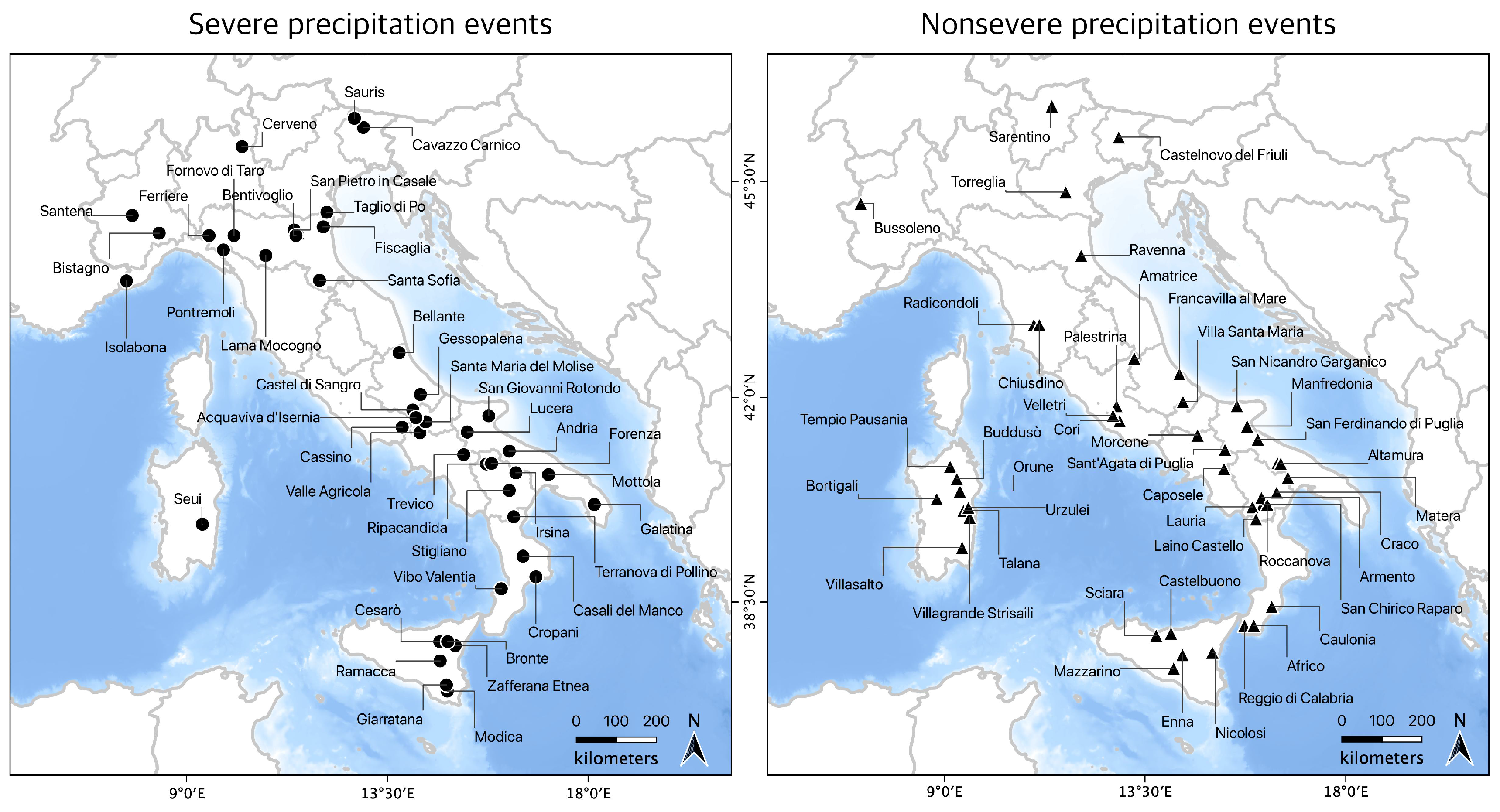
| Date | Time [UTC] | (Lat,Lon) [,] |
|---|---|---|
| 23 June 2016 | 12:00–13:00 | (40.43,16.23) |
| 26 June 2016 | 15:00–16:00 | (44.73,11.41) |
| 1 July 2016 | 12:00–13:00 | (41.79,14.07) |
| 1 July 2016 | 16:00–17:00 | (44.64,11.49) |
| 5 July 2016 | 14:00–15:00 | (44.64,10.06) |
| 9 August 2016 | 5:00–6:00 | (38.73,16.05) |
| 2 September 2016 | 14:00–15:00 | (44.64,9.5) |
| 1 June 2017 | 15:00–16:00 | (44.96,7.78) |
| 16 June 2017 | 14:00–15:00 | (44.41,9.82) |
| 17 June 2017 | 12:00–13:00 | (41.41,14.23) |
| 21 June 2017 | 14:00–15:00 | (41.04,15.21) |
| 22 June 2017 | 12:00–13:00 | (41.59,14.36) |
| 23 June 2017 | 14:00–15:00 | (40.88,15.72) |
| 24 June 2017 | 13:00–14:00 | (46.04,10.24) |
| 24 June 2017 | 14:00–15:00 | (41.42,15.29) |
| 24 June 2017 | 15:00–16:00 | (40.89,15.83) |
| 25 June 2017 | 10:00–11:00 | (45.01,12.14) |
| 25 June 2017 | 11:00–12:00 | (44.64,11.45) |
| 26 June 2017 | 13:00–14:00 | (44.32,10.77) |
| 2 July 2017 | 12:00–13:00 | (42.74,13.76) |
| 07 July 2017 | 13:00–14:00 | (46.34,12.96) |
| 15 July 2017 | 13:00–14:00 | (41.5,13.83) |
| 2 August 2017 | 15:00–16:00 | (46.48,12.76) |
| 7 August 2017 | 12:00–13:00 | (39.98,16.33) |
| 7 August 2017 | 15:00–16:00 | (39.30,16.54) |
| 8 August 2017 | 14:00–15:00 | (37.73,15.02) |
| 8 August 2017 | 14:00–15:00 | (37.80,14.67) |
| 8 August 2017 | 14:00–15:00 | (39.30,16.54) |
| 28 August 2017 | 15:00–16:00 | (41.66,14.14) |
| 29 August 2017 | 13:00–14:00 | (38.94,16.83) |
| 2 June 2018 | 11:00–12:00 | (40.70,17.11) |
| 22 June 2018 | 11:00–12:00 | (37.80,14.85) |
| 23 June 2018 | 15:00–16:00 | (39.85,9.35) |
| 3 August 2018 | 11:00–12:00 | (36.92,14.84) |
| 3 August 2018 | 11:00–12:00 | (42.05,14.24) |
| 3 August 2018 | 11:00–12:00 | (43.91,7.65) |
| 9 August 2018 | 11:00–12:00 | (41.10,16.23) |
| 9 August 2018 | 11:00–12:00 | (44.68,8.38) |
| 9 August 2018 | 12:00–13:00 | (44.78,12.06) |
| 9 August 2018 | 13:00–14:00 | (37.03,14.82) |
| 19 August 2018 | 11:00–12:00 | (41.69,15.77) |
| 01 June 2019 | 11:00–12:00 | (40.19,18.14) |
| 04 June 2019 | 12:00–13:00 | (43.92,11.98) |
| 08 June 2019 | 12:00–13:00 | (37.46,14.68) |
| 18 June 2019 | 12:00–13:00 | (40.73,16.38) |
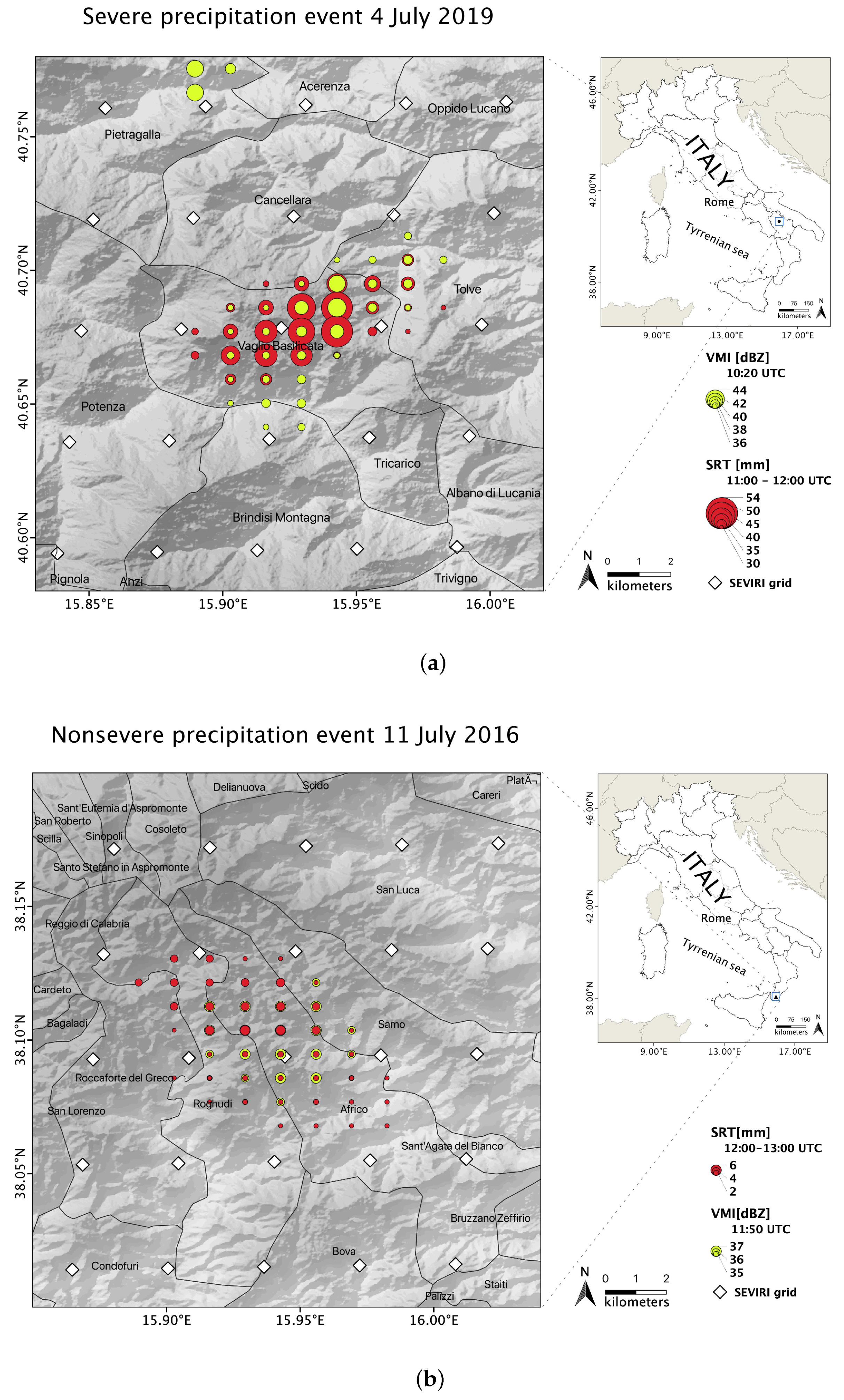
| 04 July 2019 | 11:00–12:00 | (41.73,15.89) |
| 04 July 2019 | 11:00–12:00 | (40.68,15.96) |
| 26 August 2019 | 10:00–11:00 | (37.19,14.84) |
| Date | Time [UTC] | (Lat,Lon) [,] |
|---|---|---|
| 7 June 2016 | 11:00–12:00 | (41.52,15.79) |
| 28 June 2016 | 5:00–6:00 | (42.39,14.27) |
| 1 July 2016 | 15:00–16:00 | (40.09,9.43) |
| 2 July 2016 | 14:00–15:00 | (39.97,9.57) |
| 3 July 2016 | 11:00–12:00 | (37.61,15.01) |
| 4 July 2016 | 10:00–11:00 | (38.09,15.73) |
| 7 July 2016 | 13:00–14:00 | (43.20,11.01) |
| 9 July 2016 | 17:00–18:00 | (40.40,16.45) |
| 11 July 2016 | 12:00–13:00 | (38.09,15.94) |
| 12 July 2016 | 13:00–14:00 | (40.90,16.47) |
| 30 July 2016 | 16:00–17:00 | (41.13,15.29) |
| 31 July 2016 | 16:00–17:00 | (40.19,16.13) |
| 1 August 2016 | 12:00–13:00 | (40.65,16.70) |
| 2 August 2016 | 13:00–14:00 | (41.61,12.93) |
| 4 August 2016 | 14:00–15:00 | (41.86,12.86) |
| 6 August 2016 | 14:00–15:00 | (37.91,13.75) |
| 6 August 2016 | 15:00–16:00 | (37.95,14.08) |
| 10 August 2016 | 15:00–16:00 | (44.32,12.07) |
| 1 June 2017 | 14:00–15:00 | (40.84,9.13) |
| 1 June 2017 | 16:00–17:00 | (40.42,9.35) |
| 3 June 2017 | 12:00–13:00 | (41.37,14.68) |
| 7 June 2017 | 14:00–15:00 | (37.33,14.14) |
| 4 July 2017 | 17:00–18:00 | (45.15,7.13) |
| 13 July 2017 | 8:00–9:00 | (46.19,12.91) |
| 13 July 2017 | 10:00–11:00 | (45.33,11.72) |
| 21 July 2017 | 15:00–16:00 | (40.31,16.11) |
| 04 August 2017 | 16:00–17:00 | (40.80,15.27) |
| 05 August 2017 | 14:00–15:00 | (40.15,15.91) |
| 08 August 2017 | 14:00–15:00 | (40.14,9.54) |
| 16 June 2018 | 11:00–12:00 | (41.30,16.03) |
| 16 June 2018 | 13:00–14:00 | (40.89,16.54) |
| 18 June 2018 | 13:00–14:00 | (40.29,8.83) |
| 19 June 2018 | 15:00–16:00 | (39.94,15.99) |
| 03 July 2018 | 13:00–14:00 | (41.86,15.56) |
| 10 August 2018 | 12:00–13:00 | (38.42,16.34) |
| 10 August 2018 | 14:00–15:00 | (39.45,9.40) |
| 22 September 2018 | 14:00–15:00 | (41.93,14.35) |
| 01 June 2019 | 11:00–12:00 | (42.65,13.26) |
| 10 June 2019 | 13:00–14:00 | (37.57,14.34) |
| 06 July 2019 | 14:00–15:00 | (40.19,16.24) |
| 20 July 2019 | 14:00–15:00 | (43.20,11.13) |
| 01 August 2019 | 15:00–16:00 | (46.67,11.41) |
| 06 August 2019 | 15:00–16:00 | (40.63,9.28) |
| 05 September 2019 | 13:00–14:00 | (41.70,12.78) |
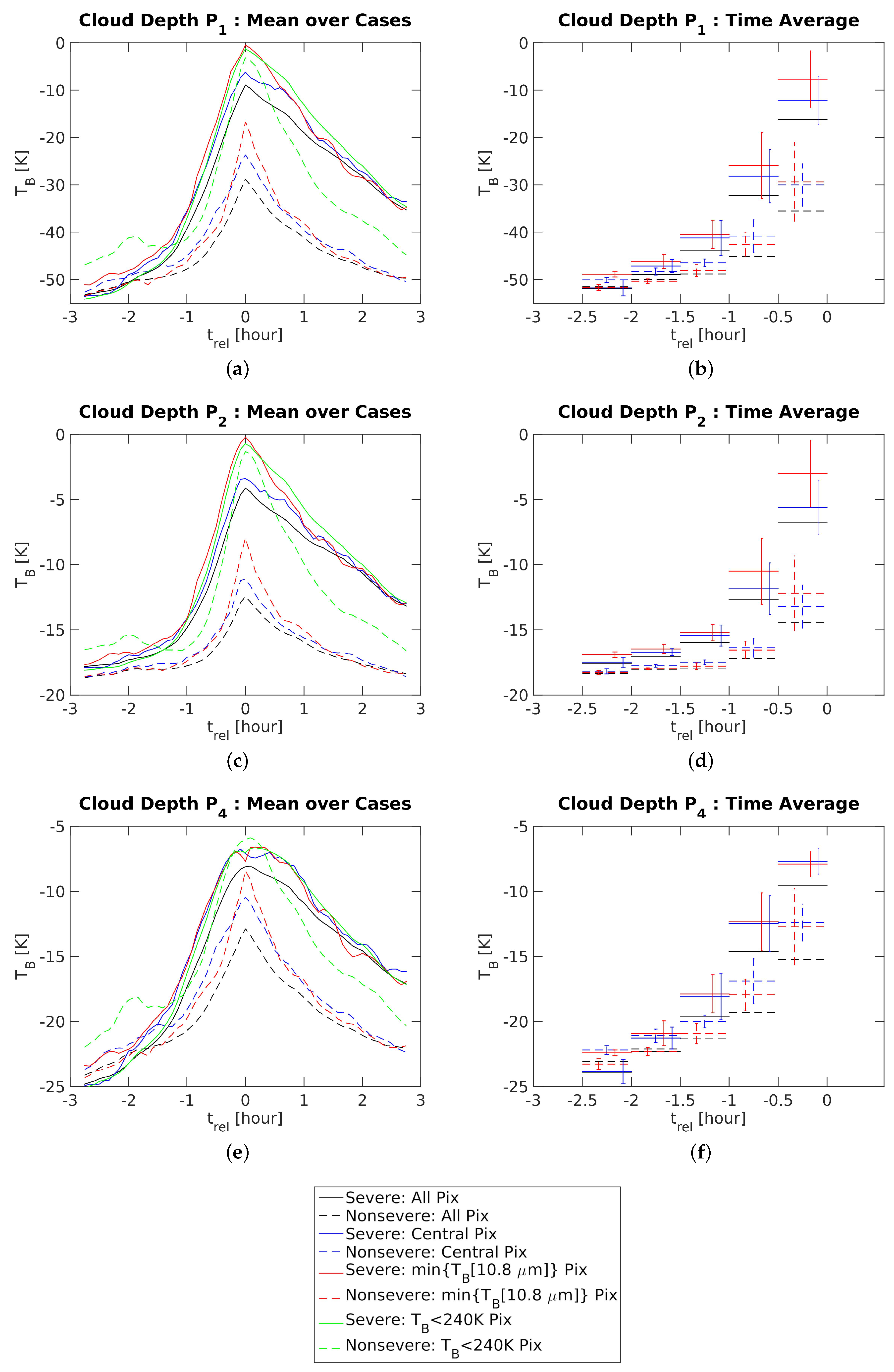
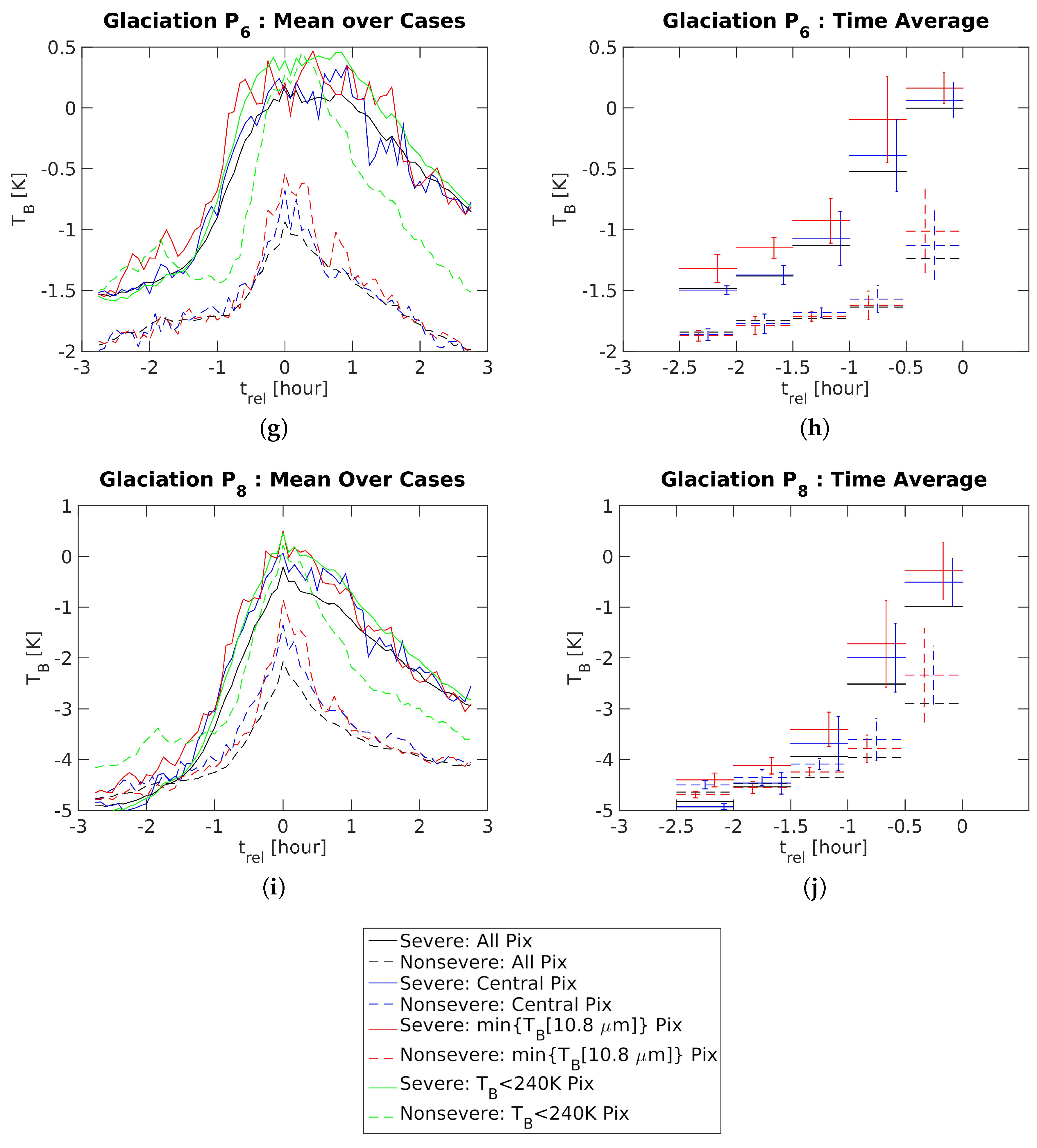
| Class | Proxy () |
|---|---|
| Cloud Depth | |
| 6.2–10.8 | |
| 6.2–7.3 | |
| 7.3–13.4 | |
| 6.2–9.7 | |
| 8.7–12 | |
| Glaciation | |
| 8.7–10.8 | |
| 5- trend: 8.7–10.8 | |
| (8.7–10.8)–(10.8–12) | |
| 5- trend: (8.7–10.8)–(10.8–12) | |
| 12–10.8 | |
| 5- trend: 12–10.8 | |
| Updraft Strength | |
| 5- trend: 6.2–7.3 | |
| 15- trend: 10.8 | |
| 10- trend: 10.8 | |
| 5- trend: 10.8 | |
| 5- trend: 6.2–10.8 | |
| 5- trend: 6.2–12 | |
| 5- trend: 9.7–13.4 |
| Time Range Prior to Storms | ACC. | POFD | POD | BIAS | |||
|---|---|---|---|---|---|---|---|
| −9.48 | −3.54 | −0.68 | 0.60 | 0.26 | 0.48 | 0.72 | |
| −27.16 | −12.12 | −1.72 | 0.63 | 0.16 | 0.43 | 0.57 | |
| −40.46 | −15.25 | −3.41 | 0.48 | 0.32 | 0.29 | 0.58 |
© 2020 by the authors. Licensee MDPI, Basel, Switzerland. This article is an open access article distributed under the terms and conditions of the Creative Commons Attribution (CC BY) license (http://creativecommons.org/licenses/by/4.0/).
Share and Cite
Gallucci, D.; De Natale, M.P.; Cimini, D.; Di Paola, F.; Gentile, S.; Geraldi, E.; Larosa, S.; Nilo, S.T.; Ricciardelli, E.; Viggiano, M.; et al. Convective Initiation Proxies for Nowcasting Precipitation Severity Using the MSG-SEVIRI Rapid Scan. Remote Sens. 2020, 12, 2562. https://0-doi-org.brum.beds.ac.uk/10.3390/rs12162562
Gallucci D, De Natale MP, Cimini D, Di Paola F, Gentile S, Geraldi E, Larosa S, Nilo ST, Ricciardelli E, Viggiano M, et al. Convective Initiation Proxies for Nowcasting Precipitation Severity Using the MSG-SEVIRI Rapid Scan. Remote Sensing. 2020; 12(16):2562. https://0-doi-org.brum.beds.ac.uk/10.3390/rs12162562
Chicago/Turabian StyleGallucci, Donatello, Maria Pia De Natale, Domenico Cimini, Francesco Di Paola, Sabrina Gentile, Edoardo Geraldi, Salvatore Larosa, Saverio Teodosio Nilo, Elisabetta Ricciardelli, Mariassunta Viggiano, and et al. 2020. "Convective Initiation Proxies for Nowcasting Precipitation Severity Using the MSG-SEVIRI Rapid Scan" Remote Sensing 12, no. 16: 2562. https://0-doi-org.brum.beds.ac.uk/10.3390/rs12162562