High-Rankness Regularized Semi-Supervised Deep Metric Learning for Remote Sensing Imagery

Abstract

Deep metric learning has recently received special attention in the field of remote sensing (RS) scene characterization, owing to its prominent capabilities for modeling distances among RS images based on their semantic information. Most of the existing deep metric learning methods exploit pairwise and triplet losses to learn the feature embeddings with the preservation of semantic-similarity, which requires the construction of image pairs and triplets based on the supervised information (e.g., class labels). However, generating such semantic annotations becomes a completely unaffordable task in large-scale RS archives, which may eventually constrain the availability of sufficient training data for this kind of models. To address this issue, we reformulate the deep metric learning scheme in a semi-supervised manner to effectively characterize RS scenes. Specifically, we aim at learning metric spaces by utilizing the supervised information from a small number of labeled RS images and exploring the potential decision boundaries for massive sets of unlabeled aerial scenes. In order to reach this goal, a joint loss function, composed of a normalized softmax loss with margin and a high-rankness regularization term, is proposed, as well as its corresponding optimization algorithm. The conducted experiments (including different state-of-the-art methods and two benchmark RS archives) validate the effectiveness of the proposed approach for RS image classification, clustering and retrieval tasks. The codes of this paper are publicly available.

1. Introduction

Nowadays, the increasing availability of remote sensing (RS) data offers widespread opportunities in many important application fields, such as urban planning [1,2,3], aerial scene retrieval [4,5,6], change detection [7,8], analysis of the earth’s surface [9,10], vegetation mapping [11,12], and remote object detection [13,14]. In these (and many other) important applications, the visual interpretation of RS scenes becomes a particularly challenging task, since a semantic characterization of RS images is required to deal with highly complex spatio-spectral land cover components that lead to high intra-class (and low inter-class) variability [15]. Note that there are specific factors affecting RS data, such as sensing conditions, sensor types, and data volume (among others) that often make semantically similar aerial scenes exhibit very different characteristics, resulting in the so-called large-scale variance problem [16,17,18].

With the improvement of earth observation technologies, different RS image characterization methods have been successfully proposed in the literature to deal with such intricacies [19]. In general, it is possible to distinguish three main types of methods: hand-crafted feature-based [20,21], unsupervised feature learning-based [22,23], and deep feature learning-based methods [24,25,26,27]. Despite the potential advantages of using manually designed features or unsupervised learning techniques, the enormous capability of deep learning models as feature extractors makes these methods the current state-of-the-art technology to effectively characterize RS scenes via convolutional neural networks (CNNs) [28,29,30,31]. Among all the conducted research, deep metric learning has recently shown to be one of the most relevant image characterization trends, since it pursues to map the input data into a feature space where semantically similar images are projected to nearby locations [32,33,34]. However, this kind of model generally demands massive amounts of annotated data for training, which may severely constrain their practical application in operational RS scenarios with limited labelled data [35].

In order to address the above-mentioned limitation, this paper proposes a novel RS image characterization method, named high-rankness regularized semi-supervised deep metric learning (HR-S²DML), which re-defines the standard deep metric learning framework by using an innovative semi-supervised design. More specifically, the proposed method aims at learning a low-dimensional metric space, which is able to capture semantic similarities among aerial scenes from a reduced number of labeled images, while exploiting the potential decision boundaries of massive unlabeled RS images. To achieve this goal, the proposed model includes a newly defined loss function, which is based on two main constitutive components: (i) a normalized softmax loss with margin, which aims at aligning RS images from the same class—as well as enhancing the intra-class compactness and inter-class discrepancy under the semi-supervised framework—and (ii) a high-rankness regularization term, which enforces the model preservation from the viewpoint of both the discrimination and diversity capabilities between labeled and unlabeled RS scenes. Additionally, an appropriate optimization mechanism is also proposed to generate consistent features within each training epoch. The extensive experimental comparison conducted in this work, including several state-of-the-art models and two benchmark datasets, validates the effectiveness of the proposed method in the task of characterizing RS scenes on three different applications: classification, clustering, and retrieval. Summarizing, the main contributions of this paper can be listed as follows:

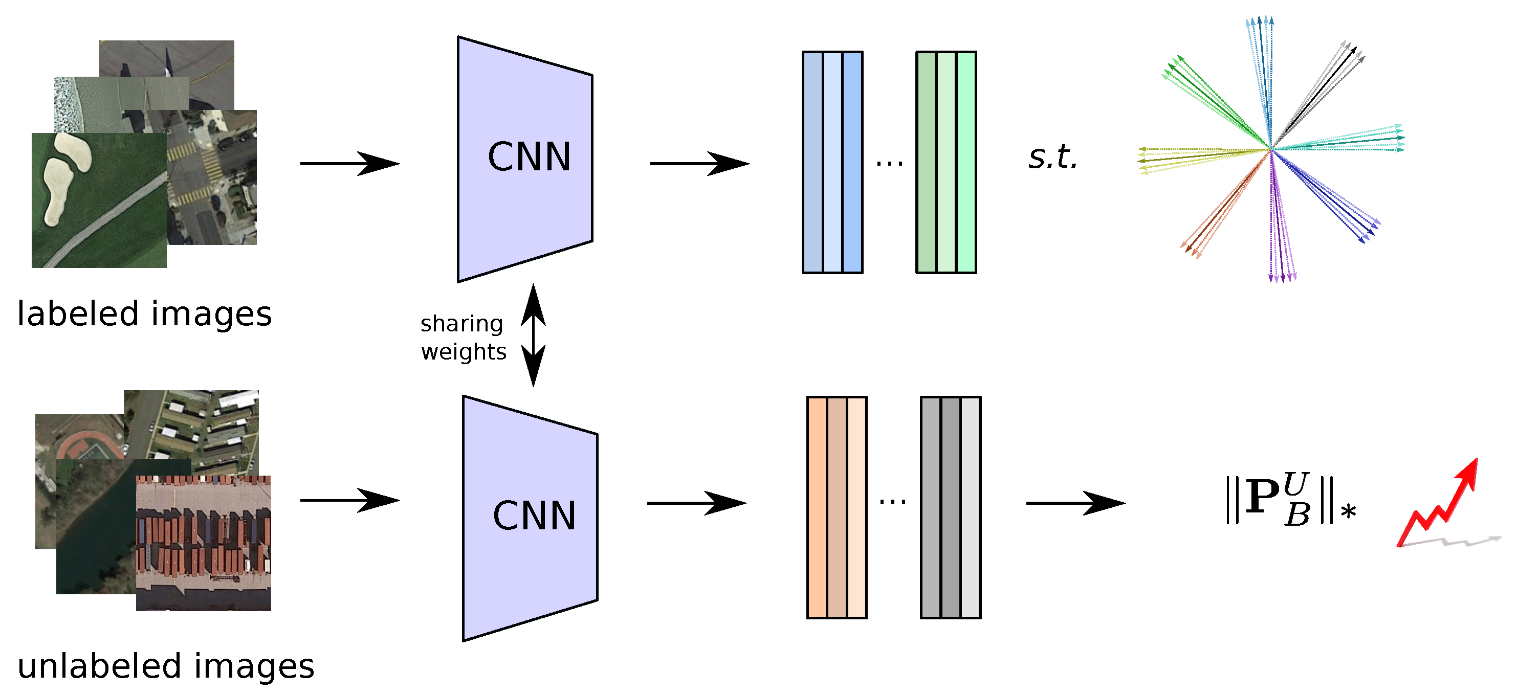
• A new semi-supervised deep metric learning model is presented to characterize vast RS image collections in an end-to-end manner, using a reduced amount of annotated data. Specifically, the proposed method has been designed to learn (based on CNN models) a metric space that jointly preserves the discrimination capability for labelled and unlabelled RS scenes.
• A new loss function, based on the normalized softmax loss with margin and the high-rankness regularization, is proposed to enhance the feature learning ability under a semi-supervised assumption. Additionally, an optimization mechanism is also defined to produce consistent features within each training epoch.
• The extensive experimental evaluation (based on three different RS applications) conducted in this paper compares the performance of the proposed method against different state-of-the-art methods using several datasets. The codes of this paper are publicly available to the research community (https://github.com/jiankang1991).

The organization of the rest of paper is the following. Section 2 introduces some related works as well as their main limitations to characterize aerial scenes. Section 3 defines the proposed semi-supervised model for efectively representing RS scenes. Section 4 presents the experimental part of the work including different benchmark datasets and state-of-the-art methods. Section 5 provides a discussion of the obtained results. Finally, Section 6 concludes the paper with some remarks and hints at plausible future research lines.

2. Related Work

During the past years, a considerable number of methods have been proposed for characterizing RS images. Generally, these approaches can be categorized into three different types [36]: hand-crafted feature-based, unsupervised feature learning-based, and end-to-end deep learning-based methods. Hand-crafted feature-based techniques make use of different visual descriptors to capture elementary image characteristics, such as color [37], shape [20,38], or texture [21,39]. Alternatively, unsupervised learning methods try to improve these results by using different kinds of unsupervised learning protocols. That is, these approaches pursue to encode the low-level visual descriptors into a higher-level feature space via sparse coding [40,41], topic modeling [42], and auto-encoders [43], among other unsupervised paradigms. However, the lack of supervised information during the learning process often reduces the ability of these techniques to effectively discriminate among complex RS concepts [19]. With the development of deep learning technology, deep learning-based methods have been shown to obtain excellent results for characterizing RS scenes, due to the great potential of CNNs to uncover high-level features from an end-to-end perspective [44]. For example, this is the case of the work in Li et al., who define in [45] a multi-layer feature fusion framework that exploits multiple pre-trained CNN models to represent RS images. Analogously, Piramanayagam et al. proposed in [46] a composite convolutional architecture to fuse multi-sensor data into a single characterization. Moreover, Li et al. presented in [30] a feature extraction network for RS that combines global and local features using the VGGNet [47] model and a recurrent neural network-based attention module, respectively. Other Authors, such as Pires et al. in [31] also showed the benefits of considering a transfer learning approach to characterize RS scenes.

Despite the advantages of these and other deep learning-based methods [48], the deep metric learning scheme has recently been shown to be one of the most effective alternatives to characterize RS data [49]. In general, deep metric learning is focused on projecting semantically similar images to nearby locations in feature space, using non-isotropic metrics [50]. Consequently, this scheme is becoming increasingly popular for alleviating the large-scale variance problem in RS since it can naturally model complex semantic similarities. For instance, Cheng et al. defined in [32] a deep metric learning approach (with a regularization term) based on the contrastive embedding framework [51] to learn discriminative CNN-based characterizations for RS images. In [33], Yan et al. developed a cross-domain extension of this contrastive scheme to reduce the bias of the corresponding feature distribution and the spectral shift. Alternative works also contemplate other relationships between RS scenes when learning the feature space. This is the case of Cao et al. who proposed in [52] a deep metric learning method for representing aerial scenes using a predefined CNN model and the triplet loss formulation [53], where both positive and negative samples are used to build the corresponding feature embeddings. Yun et al. presented in [34] a coarse-to-fine deep metric learning technique based on the triangular loss, which also accounts for the differences between negative and positive samples during training to achieve more precise results. Additionally, Kang et al. defined in [54] a deep metric learning framework for characterizing RS images based on scalable neighborhood component analysis [55], in order to better preserve the neighborhood structure in scalable datasets. Hong et al. [56] proposed a novel deep cross-modal network, which improves the classification results based on the cross-modality RS datasets.

Existing deep metric learning methods for RS image characterization are mainly focused on considering tuples of two or three labelled scenes, and then learning their binary relationships to build the corresponding feature space in a supervised manner. However, the availability of such annotations for training is usually rather limited in RS, since obtaining high-quality ground-truth land cover information for vast image archives is very expensive, as well as time-consuming. This fact logically contrasts with the requirement of large amounts of training data to properly train deep metric learning-based image characterization models, which may eventually become an important constraint in RS [18]. Although unsupervised image characterization methods [57,58] are potentially able to relieve this limitation, the high intricacy of the RS image domain still makes unsupervised schemes unable to capture the complex semantic relationships between land cover concepts, because real RS class labels are not taken into account [19]. With these considerations in mind, it seems reasonable to find a trade-off between the supervised and unsupervised scenarios in order to take advantage of both paradigms to effectively characterize RS images from a deep metric learning-based perspective. Precisely, some recent works point the benefits of using a semi-supervised scheme in this context. For example, Liu et al. defined in [59] a semi-supervised deep metric learning approach specially designed to classify synthetic aperture radar (SAR) data. More specifically, the authors made use of a manifold regularization term to penalize large distances between labeled and nearest neighbor unlabeled instances of synthetic aperture radar (SAR) data; however, the same authors concluded that there is still room for improvement since more research is required to provide effective solutions for multi-spectral RS data and other target applications. That is, the increasing complexity of RS images in terms of data volume and semantic understanding [16,18,35] demands new strategies to enhance the capacity of deep metric learning-based characterization methods to distinguish between a broader range of contrasting land cover types using limited amounts of labelled data. More precisely, relieving these important limitations (from a semi-supervised viewpoint) motivates the research conducted in this work.

3. Proposed Semi-Supervised Deep Metric Learning for Remote Sensing

The proposed HR-S²DML approach, which is specially designed to characterize RS images, is composed of two main parts: (1) a backbone CNN architecture to encode the RS images into corresponding features in a low-dimensional metric space; and (2) a new joint loss function for guiding the CNN model to learn a metric space in semi-supervised fashion. Figure 1 illustrates the proposed framework in a graphical way. As it is possible to see, the proposed end-to-end model is made up of two different segments that make use of the same CNN backbone architecture and share their corresponding weights. On the one hand, the top segment covers the labeled RS scenes by the normalized softmax loss with margin, with the objective of facilitating the generation of a metric space with high intra-class compactness and inter-class discrepancy for the available labelled data. On the other hand, the bottom segment employs the high-rankness regularization over the unlabelled images for preserving the discrimination and diversity capabilities on the unlabeled data. The details of our approach will be provided in the following subsections. Nonetheless, we first briefly define the notations used in the paper.

Let us assume that L and U represent labelled and unlabelled images, respectively. Let ${\mathcal{X}}^L=\{{\mathbf{x}}_1^L,\cdots ,{\mathbf{x}}_{M^L}^L\}$ be an RS image dataset of $M^L$ images with category annotations, and $\mathcal{Y}=\{{\mathbf{y}}_1^L,\cdots ,{\mathbf{y}}_{M^L}^L\}$ be the corresponding set of labels, where each label is represented by a one-hot vector of the form ${\mathbf{y}}_i^L\in {\{0,1\}}^C$, being C the number of classes. That is, the c-th component of ${\mathbf{y}}_i^L$ is 1 (i.e., $y_i^c=1$) when the image ${\mathbf{x}}_i$ is annotated with class c. ${\mathcal{X}}^U=\{{\mathbf{x}}_1^U,\cdots ,{\mathbf{x}}_{M^U}^U\}$ denotes the unlabeled RS image dataset, where $M^L\ll M^U$. deep metric learning aims to learn a CNN model $\mathcal{F}(·)$ for effectively encoding the semantic contents of images with low-dimensional feature embeddings in the produced metric space, where the semantically similar images are located close and semantically dissimilar images are separated. In the context of semi-supervised deep metric learning, the CNN model $\mathcal{F}(·)$ is learned by utilizing both the labeled and unlabeled image datasets, ${\mathcal{X}}^L$ and ${\mathcal{X}}^U$. With respect to the image ${\mathbf{x}}_i$, ${\mathbf{f}}_i\in {\mathbb{R}}^D$ represents its normalized feature embedding produced by $\mathcal{F}(·)$, i.e., ${\mathbf{f}}_i=\mathcal{F}\left({\mathbf{x}}_i\right)/{\parallel \mathcal{F}\left({\mathbf{x}}_i\right)\parallel }_2$, and D is the dimension of the feature embedding. Using this notation, the following subsections describe the different parts of the proposed joint loss function and the optimization algorithm.

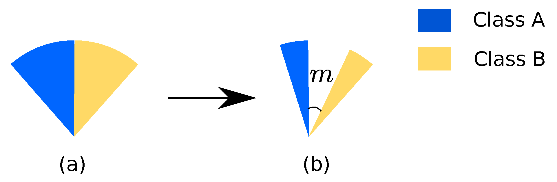
3.1. Normalized Softmax Loss with Margin

The softmax loss, also noted as cross-entropy loss, is widely applied for supervised classification:

$${\mathcal{L}}_{\mathrm{s}}=-\frac{1}{M^L}\sum _i\sum _c{y}_i^{c}log\left(p_i^c\right),$$

(1)

where $M^L$ represents the number of labeled images, and $p_i^c$ represents the probability that ${\mathbf{x}}_i^L$ is classified into class c, described by:

$$p_i^c=\frac{e^{{\mathbf{w}}_c^T\mathcal{F}\left({\mathbf{x}}_i^L\right)}}{{\sum }_k{e}^{{\mathbf{w}}_k^T\mathcal{F}\left({\mathbf{x}}_i^L\right)}},$$

(2)

where ${\mathbf{w}}_c\in {\mathbb{R}}^D$ denotes the learnable weight vector associated with the class c. Here, the bias term is omitted for simplicity. By minimizing the softmax loss, the images from the same class are aligned with respect to the corresponding weight vector ${\mathbf{w}}_c$ [54,55]. However, the similarity for intra-class images and the diversity for inter-class images cannot be explicitly enforced by the softmax loss [60]. Thus, the metric space produced via the CNN model optimized by the softmax loss cannot sufficiently capture the semantic structures among the images, especially under a semi-supervised learning framework. To overcome such limitation, we utilize the normalized softmax loss with margin to enhance the intra-class compactness and inter-class discrepancy [60]. Specifically, with the assumption that ${\mathbf{w}}_c$ is normalized, i.e., $\parallel {\mathbf{w}}_c{\parallel }_2=1$, the loss function can be described as:

$${\mathcal{L}}_{\mathrm{s}-\mathrm{m}}=-\frac{1}{M^L}\sum _{i}log\frac{e^{\frac{cos({\theta }_i^c+m)}{\tau }}}{e^{\frac{cos({\theta }_i^c+m)}{\tau }}+{\sum }_{k,k\ne c}{e}^{\frac{cos\left({\theta }_i^k\right)}{\tau }}},$$

(3)

where ${\theta }_i^c$ denotes the angular margin between the feature embedding ${\mathbf{f}}_i^L$ and ${\mathbf{w}}_c$, i.e., ${\theta }_i^c=arccos\left({\mathbf{w}}_c^T{\mathbf{f}}_i^L\right)$, m is the angular margin penalty, and $\tau$ represents the temperature parameter which regulates the level of concentration in the sample distribution [61]. Compared with the traditional softmax loss, the involved angular margin penalty m can enforce the images from the same class to be closer to each other and the images from different classes to be pushed away. The effect of the angular margin can be illustrated in Figure 2. By minimizing the traditional softmax loss, the feature embeddings within each class are optimized to decrease their cosine distances with respect to the corresponding class prototype vector ${\mathbf{w}}_c$. Therefore, they are enforced to be aligned with respect to each class prototype learned by the CNN model. However, the image features from different classes lying around the class decision boundaries may still share some similarities. Given such a learned metric space, the out-of-sample images located near such class boundaries cannot be easily categorized. By exploiting the normalized softmax loss with margin, we encourage that the images belonging to different classes are forced to be separated with a certain angular distance, so that the semantic structure of the metric space can be better characterized by the learned CNN model.

3.2. High-Rankness Regularization

Although the metrics for the labeled images can be captured by using the normalized softmax loss with margin, the discrepancy between the labeled training images and the unlabeled test images could lead to a poor prediction performance under a semi-supervised learning scenario. Since the CNN model is optimized using just a small number of labelled images, the learned decision boundaries with respect to the unseen test images are often ambiguous. Moreover, in case of the CNN model trained by an unbalanced dataset, it is normal that a few categories dominate the images within mini-batches, which can degrade the prediction diversity of the trained CNN model. In order to overcome these limitations, we adopt the high-rankness regularization of the model predictions within each mini-batch to enforce the optimized CNN model with the preservation of both the discrimination and diversity capabilities [62]. Specifically, given each mini-batch of unlabeled images ${\mathbf{X}}_B^U$, the rank of their category prediction matrix is maximized as:

$$max\left(\mathrm{Rank}\left({\mathbf{P}}_B^U\right)\right),$$

(4)

where ${\mathbf{P}}_B^U$ is the probability matrix of the category prediction for each mini-batch. Such optimization is an NP-hard non-convex problem. The rank optimization can also be relaxed into the optimization of matrix nuclear norm [63,64,65,66,67,68]. Thus, Equation (4) can be relaxed by minimizing the following loss function:

$${\mathcal{L}}_{\mathrm{HR}}=-{\parallel {\mathbf{P}}_B^U\parallel }_{*}.$$

(5)

This optimization increases the rankness of the predicted class probability matrix of each mini-batch ${\mathbf{P}}_B^U$. As ${\mathbf{P}}_B^U$ can be described by:

$${\mathbf{P}}_B^U=\frac{e^{{\mathbf{W}}^T\mathcal{F}\left({\mathbf{X}}^U\right)}}{{\sum }_c{e}^{{\mathbf{W}}^T\mathcal{F}\left({\mathbf{X}}^U\right)}},$$

(6)

where ${\sum }_c(·)$ denotes a summation along the category direction. In the case of semi-supervised learning, the classification of a large amount of unlabeled images based on the learned class prototype $\mathbf{W}$ with a limited number of training images may not be sufficient. Thus, most feature embeddings of unlabeled images may be located around the class decision boundaries. In other words, the predicted class probability vectors of unlabeled images from different classes are similar to each other. This leads to the low-rankness of the matrix ${\mathbf{P}}_B^U$ and, inevitably, to classification ambiguities for the unlabeled images. By minimizing ${\mathcal{L}}_{\mathrm{HR}}$, the feature embeddings of the unlabeled images will be pushed towards the learned class prototypes $\mathbf{W}$, and the discrimination and diversity capabilities of the CNN model on massive unlabeled images can be preserved. To this end, the proposed joint loss function for training the CNN model is formulated as:

$$\mathcal{L}={\mathcal{L}}_{\mathrm{s}-\mathrm{m}}+\lambda {\mathcal{L}}_{\mathrm{HR}}.$$

(7)

Finally, the corresponding optimization algorithm is described in Algorithm 1.

Algorithm 1 Optimization for HR-S2DML

Require:${\mathbf{x}}_i^L$, ${\mathbf{x}}_i^U$, and ${\mathbf{y}}_i^L$

1: Initialize $\tau$, m, $\lambda$ and D

2: for $t=0$ to $\mathrm{maxEpoch}$ do

3:  Sample mini-batches from training and test sets, ${\mathbf{X}}_B^L$ and ${\mathbf{X}}_B^U$.

4:  ${\mathcal{L}}_{\mathrm{s}-\mathrm{m}}$ and ${\mathcal{L}}_{\mathrm{HR}}$ based on ${\mathbf{X}}_B^L$ and ${\mathbf{X}}_B^U$, respectively.

5:  Aggregate the two loss terms into a joint loss $\mathcal{L}$.

6:  Calculate the gradients and do back-propagation.

7: end for

Ensure:$\mathcal{F}(·)$

4. Experiments

4.1. Dataset Description

To validate the performance of the proposed semi-supervised deep metric learning approach, this work considers two benchmark RS image archives. A detailed description of these datasets is provided below:

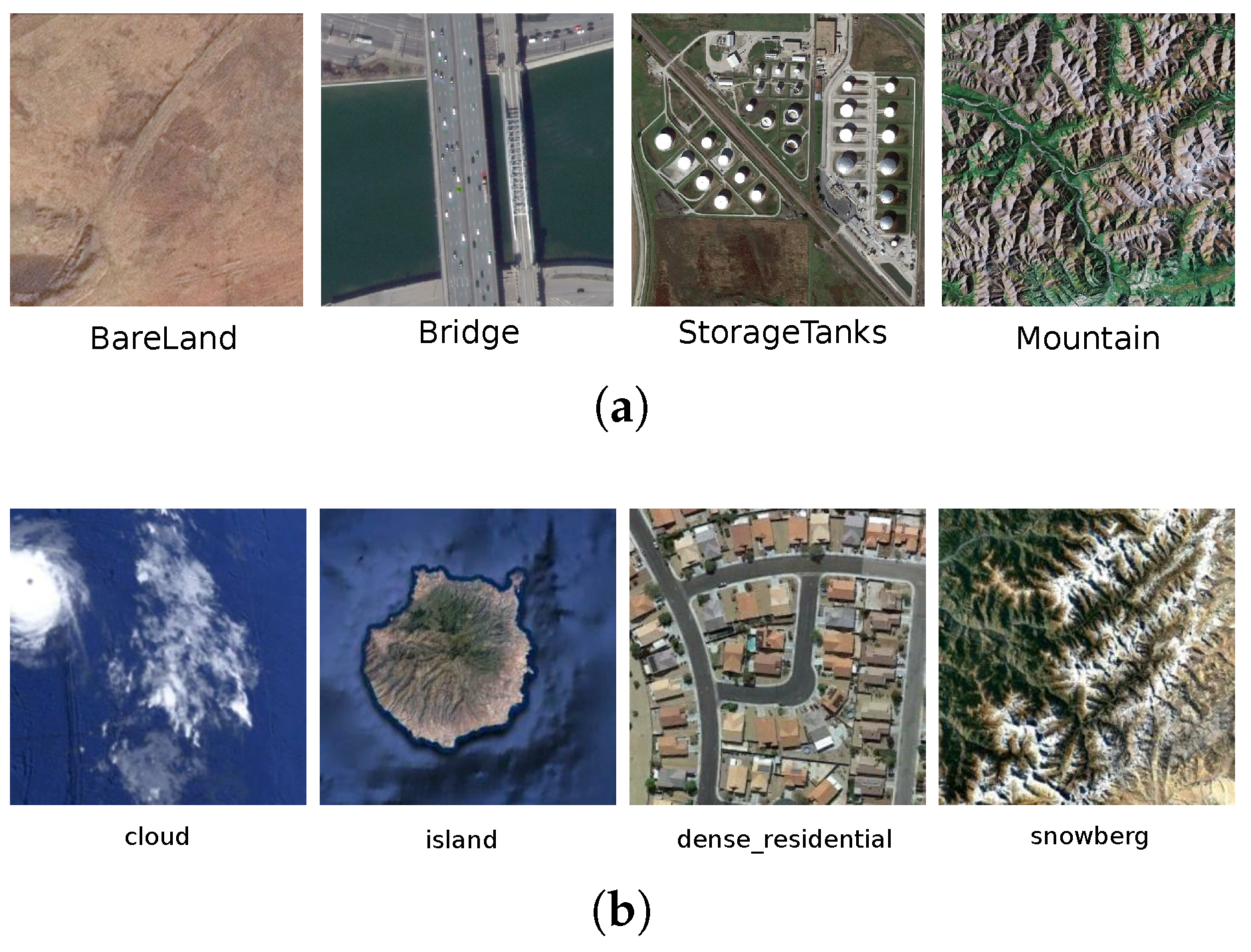
• Aerial Image Dataset (AID) [69]: This dataset has been specifically designed for RS image classification and retrieval tasks. Specifically, it contains a total of 10,000 images belonging to the following 30 semantic classes: airport, bare land, baseball field, beach, bridge, center, church, commercial, dense residential, desert, farmland, forest, industrial, meadow, medium residential, mountain, park, parking, playground, pond, port, railway station, resort, river, school, sparse residential, square, stadium, storage tanks, and viaduct. Figure 3a shows some of its images for illustrative purposes. All the images have a size of $600\times 600$ pixels in the RGB space, with a spatial resolution ranging from 8 to 0.5 meters, and each semantic class contains from 220 to 420 images. This collection is available online (AID: https://captain-whu.github.io/AID/).
• NWPU-RESISC45 [19]: This archive is a large-scale RS dataset, which is made of 31,500 images which are uniformly distributed in the following 45 semantic classes: airplane, airport, baseball diamond, basketball court, beach, bridge, chaparral, church, circular farmland, cloud, commercial area, dense residential, desert, forest, freeway, golf course, ground track field, harbor, industrial area, intersection, island, lake, meadow, medium residential, mobile home park, mountain, overpass, palace, parking lot, railway, railway station, rectangular farmland, river, roundabout, runway, sea ice, ship, snow-berg, sparse residential, stadium, storage tank, tennis court, terrace, thermal power station, and wetland. Figure 3b illustrates some examples of this collection. All the images have a size of $256\times 256$ pixels in the RGB space, with a spatial resolution varying from 30 to 0.2 m. This dataset is also available online (NWPU-RESISC45: http://www.escience.cn/people/JunweiHan/NWPU-RESISC45.html).

In order to generate a semi-supervised learning scenario for the experimental part of the work, we randomly select for each dataset a $5\%$, $10\%$, $15\%$ and $20\%$ of the data as labeled images, and a $95\%$, $90\%$, $85\%$ and $80\%$ as unlabeled images, respectively. Note that we also identify these sets of labeled and unlabeled images as training and test sets in the downstream evaluation tasks.

These RS archives have been selected as benchmark collections due to their challenging complexity (in terms of data volume, semantic intricacy and visual diversity) and also their widespread popularity in other related works [32,33,54]. However, alternative RS datasets with different spectral bands could be used instead by adjusting the number of channels of the considered backbone architecture to the number of bands of the input data.

4.2. Evaluation Tasks

For evaluating the effectiveness of the proposed method on the feature embedding generation, we conduct experiments related to three different RS tasks: (1) KNN classification; (2) clustering; and (3) image retrieval.

4.2.1. KNN Classification

Given an out-of-sample image identified by ${\mathbf{x}}^{*}$, its corresponding feature embedding ${\mathbf{f}}^{*}$ can be generated using the trained CNN model $\mathcal{F}(·)$. By measuring the Euclidean distance between ${\mathbf{f}}^{*}$ and the feature embeddings of the training set in the metric space, the top-K nearest neighbors can be retrieved. Then, based on the majority voting of the labels associated with the K nearest neighbors, ${\mathbf{y}}^{*}$ can be calculated. The performance evaluation is done by calculating the overall accuracy figure of merit.

4.2.2. Clustering

The generated feature embeddings of the test set can also be evaluated by carrying out k-means clustering. If they can be perfectly clustered in the metric space, the uncovered clusters can match the ground-truth semantic classes. For the performance evaluation, we exploit the Normalized Mutual Information (NMI) and the unsupervised clustering accuracy (ACC) [70]. NMI is defined by:

$$\mathrm{NMI}=\frac{2\times I(\mathbf{Y};\mathbf{C})}{H\left(\mathbf{Y}\right)+H\left(\mathbf{C}\right)}.$$

(8)

In this expression, $\mathbf{Y}$ denotes the ground-truth labels and $\mathbf{C}$ represents the corresponding cluster assignments. Besides, $I(·;·)$ and $H(·)$ are the mutual information and entropy functions, respectively. This figure of merit quantifies the agreement between the ground-truth information and the assigned clusters. For ACC, it is defined by:

$$\mathrm{ACC}=\underset{\mathcal{M}}{max}\frac{{\sum }_{i=1}^N\delta (l_i=\mathcal{M}\left(c_i\right))}{M^U},$$

(9)

where $l_i$ denotes the ground-truth class, $c_i$ is the assigned cluster of image ${\mathbf{x}}_i^U$ and being $\delta (·)$ the Dirac delta function. Additionally, $\mathcal{M}$ represents a mapping function than finds the best correspondence between the uncovered clusters and the ground-truth classes.

4.2.3. Image Retrieval

Given the feature embedding of one query image, the image retrieval task aims to find the images in the dataset with high semantic-similarity. Such similarity can be measured by the Euclidean or Cosine distance between the feature embedding of the query image and the ones in the dataset. Logically, the more effective the metric learning technique, the more semantically relevant the images retrieved from its embedding space. For assessment purposes, we make use of the Precision-Recall (PR) curve to analyze the precision and recall metrics when varying the total number of retrieved images and the mean average precision (MAP). The average precision (AP) is defined by:

$$\mathrm{AP}=\frac{1}{Q}\sum _{r=1}^{R}P\left(r\right)\delta \left(r\right),$$

(10)

where Q is the number of ground-truth RS images in the dataset that are relevant with respect to the query image, $P\left(r\right)$ denotes the precision for the top r retrieved images, and $\delta \left(r\right)$ is an indicator function to specify whether the rth relevant image is truly relevant to the query.

4.3. Experimental Setup

As it was previously mentioned, the semi-supervised learning scheme is generated by randomly selecting $5\%$, $10\%$, $15\%$ and $20\%$ of the datasets as labeled images (training) and the remaining samples as unlabeled data (test). After fixing these partitions for each dataset, we train the models (once per considered ratio) and perform the corresponding evaluation tasks. The clustering task is conducted on the feature embeddings of the test sets generated by the learned CNN model. For image retrieval purposes, the test set is served for querying, and the training set is the database. The proposed method is implemented in PyTorch [71]. We use ResNet18 [72] as the CNN backbone for extracting the features. It is worth noting that other CNN architectures can also be applied, while we exploit ResNet18 in this paper for the sake of simplicity. The images are all resized to $256\times 256$ pixels, and three data augmentation methods are adopted during training: (1) RandomGrayscale, (2) ColorJitter, and (3) RandomHorizontalFlip. For the parameters in our HR-S²DML, we select $\tau$, m, D, and $\lambda$ to be $0.05$, $0.5$, 128 and $1.0$, respectively. The Stochastic Gradient Descent (SGD) optimizer is adopted for training. The initial learning rate is set to ${10}^{-3}$, and it is decayed by $0.5$ every 30 epochs. The batch size is 256 and we totally train the CNN model for 100 epochs. For evaluating the effectiveness of the proposed semi-supervised deep metric learning, we compare it with respect to several metric learning methods including: (1) D-CNN [32]; (2) deep metric learning based on triplet loss [52,53]—simply termed as Triplet hereinafter—; and (3) Normalized Softmax Loss (NSL) [73]. D-CNN is one of the first works for deep metric learning based on remote sensing images, where a metric learning regularizer is integrated with the cross entropy loss for learning the discriminate features. Triplet is one of the most popular losses for deep metric learning, where a triplet of images (one positive image pair and one negative image pair) is constructed for learning the metrics. NSL is exploited for learning the class proxies based on the normalized weights within the framework of the cross entropy loss, and optimizing the metrics of the input images with respect to them. Regarding their parameter configurations, the margin parameter of the triplet loss is selected as $0.2$ and the parameters of D-CNN are set to the same values as in the original paper. Additionally, the learning rates of all the compared methods are tuned to be optimal. All the experiments are conducted on an NVIDIA Tesla P100 graphics processing unit (GPU).

4.4. Experimental Results

4.4.1. KNN Classification

Table 1. KNN classification accuracies (%) obtained by using the considered methods, when the percentages of the labeled images are $5\%$, $10\%$, $15\%$, and $20\%$, respectively, and $K=10$.

	AID				NWPU-RESISC45
	5%	10%	15%	20%	5%	10%	15%	20%
D-CNN	80.03	86.62	90.22	91.61	80.08	86.06	89.21	90.75
Triplet	79.46	85.72	89.47	91.24	78.08	84.43	87.43	89.58
NSL	73.92	82.71	86.78	89.55	73.92	82.71	86.78	89.55
HR-S2DML	$\mathbf{83.19}$	$\mathbf{89.28}$	$\mathbf{92.29}$	$\mathbf{93.31}$	$\mathbf{82.46}$	$\mathbf{88.02}$	$\mathbf{90.41}$	$\mathbf{91.81}$

displays the KNN classification accuracies (%) obtained by using all the considered methods, when the percentages of the labeled images are $5\%$, $10\%$, $15\%$, and $20\%$, respectively, and $K=10$. Compared with other state-of-the-art methods, our HR-S²DML achieves the best performance on the two considered benchmark datasets. As it is posibble to observe, the proposed approach improves the classification accuracy by a margin of $10\%$ and $3\%$ with respect to NSL and D-CNN, respectively. In NSL, the normalized softmax loss is utilized without imposing the margin between the images from different classes. Thus, for a large number of unseen RS images, the produced class decision boundaries by NSL may lead to ambiguous predictions. The contrastive and triplet losses exploited in D-CNN and Triplet require a sufficient optimization when the number of training images is at the level of $\mathcal{O}\left(\right|{\mathcal{X}}^L{|}^2)$ and $\mathcal{O}\left(\right|{\mathcal{X}}^L{|}^3)$. Normally, such requirement cannot be easily satisfied when the CNN model is trained with a certain number of epochs. Thus, the performances of D-CNN and Triplet are limited by the dataset sampling. By enforcing the discrimination and diversity capabilities for both the labeled and unlabeled RS scenes, our HR-S²DML can better generate a low-dimensional metric space where the distances among the images are more accurately captured than the other tested methods.

4.4.2. Clustering

Table 2. NMI assessment (%) for the test set embeddings of the different methods, when the percentages of labeled images are $5\%$, $10\%$, $15\%$, and $20\%$, respectively.

	AID				NWPU-RESISC45
	5%	10%	15%	20%	5%	10%	15%	20%
D-CNN	72.90	79.87	82.95	86.04	72.73	79.11	81.62	84.24
Triplet	74.90	80.97	84.30	85.68	73.06	78.57	81.05	83.41
NSL	67.31	75.66	79.77	83.72	65.94	73.44	77.98	80.77
HR-S${}^2$DML	$\mathbf{78.45}$	$\mathbf{85.31}$	$\mathbf{88.59}$	$\mathbf{90.07}$	$\mathbf{78.18}$	$\mathbf{84.12}$	$\mathbf{86.69}$	$\mathbf{88.42}$

and

Table 3. ACC assessment (%) for the test set embeddings of the different methods, when the percentages of labeled images are $5\%$, $10\%$, $15\%$, and $20\%$, respectively.

	AID				NWPU-RESISC45
	5%	10%	15%	20%	5%	10%	15%	20%
D-CNN	73.87	82.26	85.91	86.24	73.67	81.66	84.38	86.30
Triplet	77.93	82.38	85.73	90.08	72.82	80.87	82.89	85.60
NSL	66.61	78.63	80.59	88.48	56.80	62.16	67.12	69.36
HR-S${}^2$DML	$\mathbf{81.87}$	$\mathbf{89.62}$	$\mathbf{92.32}$	$\mathbf{93.42}$	$\mathbf{81.61}$	$\mathbf{88.05}$	$\mathbf{90.33}$	$\mathbf{91.77}$

demonstrate the NMI and ACC scores obtained on the test sets after conducting K-means clustering to their feature embeddings generated by the different methods. It can be observed that the proposed method provides the most accurate matching between the ground-truth semantic labels and the obtained clusters. This fact indicates that the intra-class distances among the produced feature embeddings of the same class by our HR-S²DML are smaller than those obtained by the other tested methods. Moreover, the corresponding inter-class distances among the produced feature embeddings of different classes by our HR-S²DML are larger than those obtained by the other methods, so that more test images can be accurately clustered. Moreover, in Figure 4 we display the feature emebddings projected into the 2-D space via t-SNE on the AID test set. It can be obviously seen that the intra-class compactness of HR-S²DML is higher than the other considered methods, and larger margin exists for inter-class feature embeddings. From this perspective, higher clustering accuracy can be guaranteed by the proposed method.

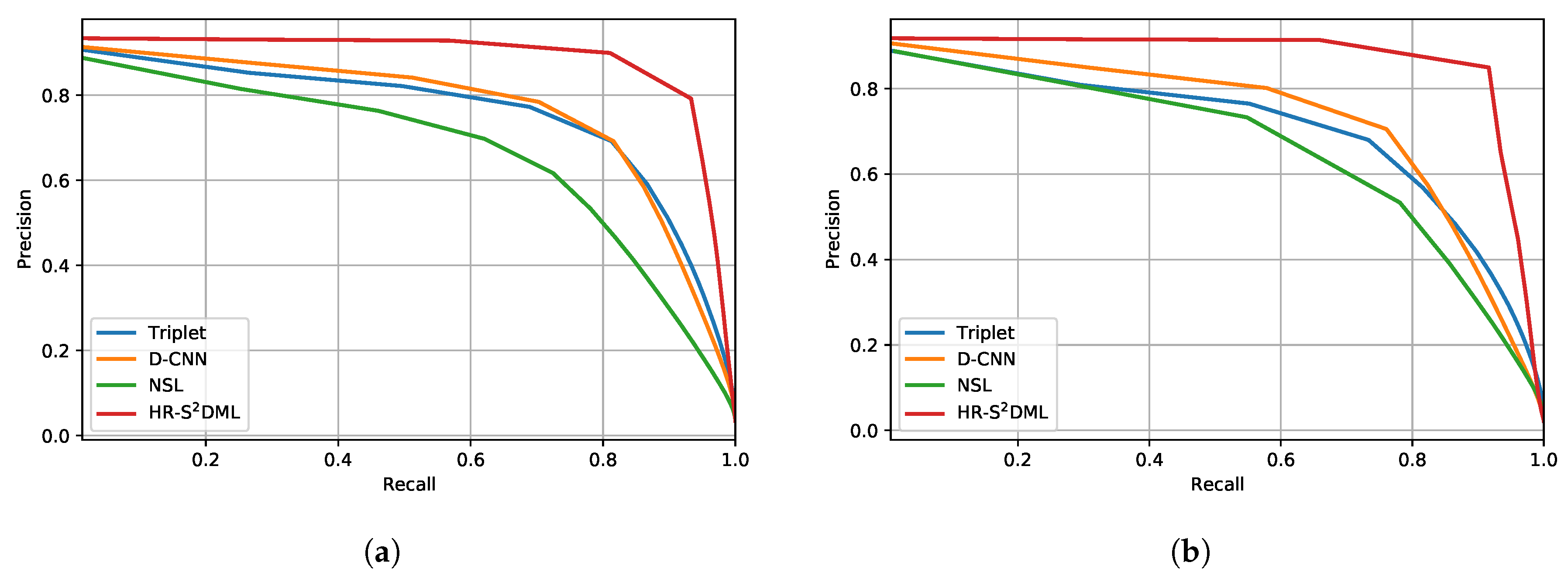
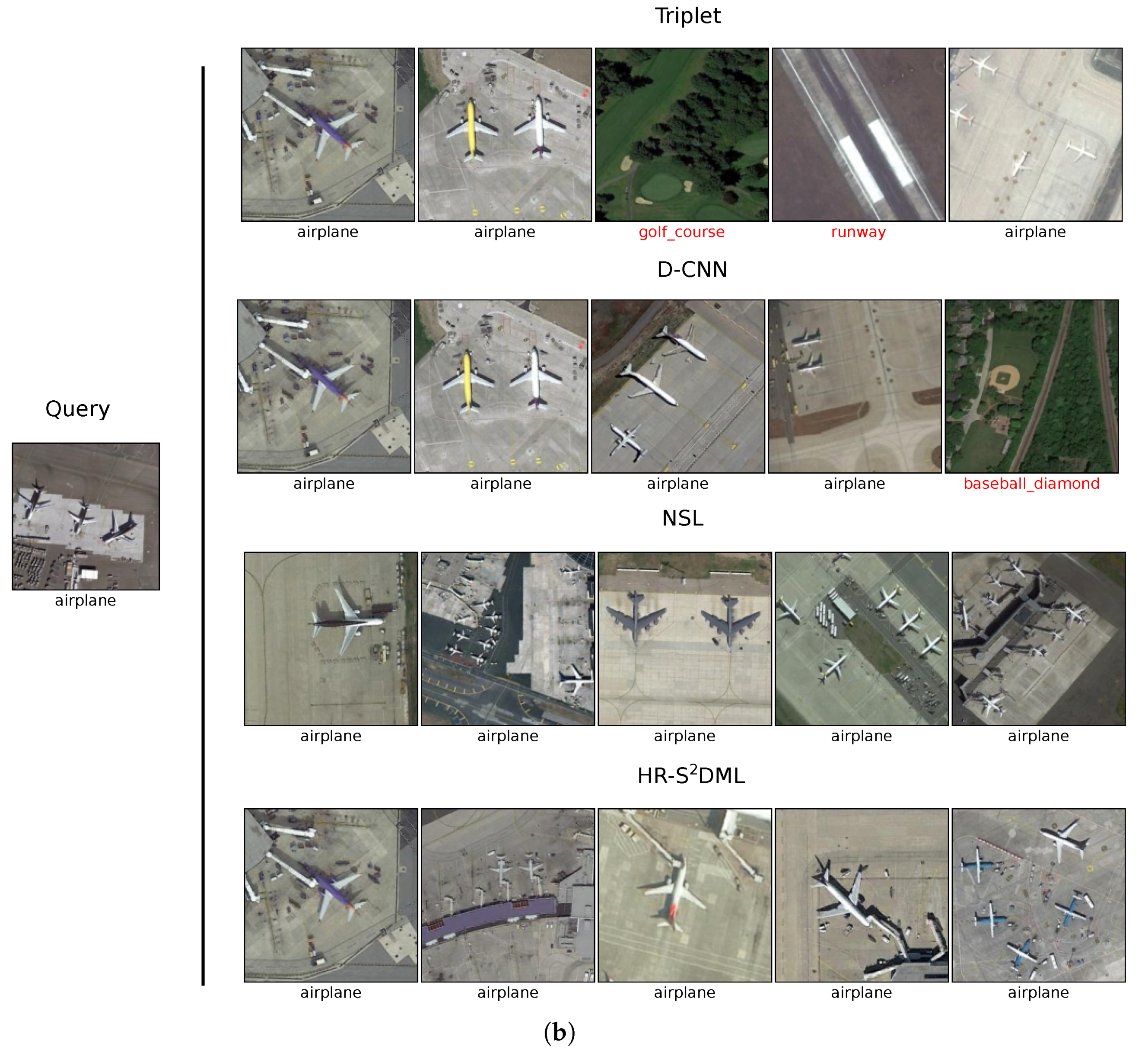
4.4.3. Image Retrieval

Figure 5 displays the PR curves showing the precision and recall pairs (with different numbers of retrieved images) with respect to the considered methods, when the percentage of the labeled images is set to $20\%$. As in the previous experiments, our HR-S²DML exhibits superior retrieval performance when compared to the other tested methods, particularly when the number of retrieved images increases. Therefore, the proposed method can group closer the images with higher semantic-similarities and separate the images with dissimilar patterns in the metric space. In

Table 4. MAP scores (%) of the image retrieval results obtained by the considered methods, when the percentages of the labeled images are $5\%$, $10\%$, $15\%$, and $20\%$, respectively, using $R=20$.

	AID				NWPU-RESISC45
	5%	10%	15%	20%	5%	10%	15%	20%
D-CNN	79.93	86.93	90.36	92.24	81.86	87.56	91.05	92.37
Triplet	77.11	84.90	88.46	90.69	77.33	83.85	87.15	89.18
NSL	69.86	79.92	84.74	88.40	69.86	79.92	84.74	88.40
HR-S${}^2$DML	$\mathbf{88.43}$	$\mathbf{95.05}$	$\mathbf{96.99}$	$\mathbf{97.62}$	$\mathbf{92.57}$	$\mathbf{95.95}$	$\mathbf{97.54}$	$\mathbf{97.98}$

, we calculate the MAP scores of the image retrieval results, when the percentages of the labeled images are $5\%$, $10\%$, $15\%$, and $20\%$, respectively, and using $R=20$. Consistently with the above observation, the proposed method obtains the best image retrieval performances for $R=20$. With a limited number of labeled images ($5\%$), the retrieval performances of the other methods significantly degrade. In comparison, the image retrieval performance of our HR-S²DML is more stable as the number of labeled images increases, which indicates that the learned CNN model exhibits better generalization capability. Given two query images from the benchmark datasets, we display the 1st, 5th, 10th, 15th, and 20th nearest neighbors retrieved based on the considered methods in Figure 6. For example, the pattern of Playground cannot be easily distinguished from BaseballField in the result of Triplet on the AID dataset.

4.4.4. Parameter Sensitivity Analysis

There are two main parameters that need to be set in the proposed method, i.e., $\tau$ and m, where $\tau$ controls the compactness of the sample distribution, and m is the introduced angular margin penalty.

Table 5. Analysis of the $\tau$ and m parameters on the AID dataset.

Parameters	$\mathit{m}=0.1$	$\mathit{m}=0.2$	$\mathit{m}=0.3$	$\mathit{m}=0.4$	$\mathit{m}=0.5$
$\tau =0.05$	90.44	90.58	91.34	91.38	91.40
$\tau =0.1$	90.90	91.01	91.59	92.11	91.40
$\tau =0.15$	90.70	91.38	91.21	91.27	91.27
$\tau =0.2$	91.11	90.88	90.81	91.40	91.04
$\tau =0.25$	89.85	90.10	90.08	89.95	90.38

and

Table 6. Analysis of the $\tau$ and m parameters on the NWPU-RESISC45 dataset.

Parameters	$\mathit{m}=0.1$	$\mathit{m}=0.2$	$\mathit{m}=0.3$	$\mathit{m}=0.4$	$\mathit{m}=0.5$
$\tau =0.05$	88.50	89.00	89.26	90.05	89.71
$\tau =0.1$	89.29	89.77	89.95	89.53	89.54
$\tau =0.15$	89.71	89.55	89.40	89.06	88.70
$\tau =0.2$	89.33	89.21	89.41	89.04	88.95
$\tau =0.25$	88.59	88.79	88.70	88.60	88.52

display the KNN classification performances with respect to different values of $\tau$ and m, when the percentage of the labeled images is $15\%$ and $K=10$. It can be observed that the best choice of $\tau$ lies in a range from $0.05$ to $0.2$ for the two benchmark datasets. Moreover, when m ranges from $0.2$ to $0.5$, optimal classification performance can be achieved. This indicates the effectiveness of the proposed approach, although a certain margin penalty can indeed improve the deep metric learning performance.

5. Discussion

Based on the experimental results from different tasks, we can observe that the proposed method can achieve the out-performance of the generated feature embeddings on the higher intra-class compactness and inter-class discrepancy compared with several state-of-the-art methods. The success of the proposed method lies on two points: (1) the precise metric learning for the limited number of labeled images; and (2) the modification of the learned class decision boundaries based on the high-rankness regularization of the unlabeled image features. When the percentage of the labeled images is low (e.g., $5\%$), HR-S²DML can also preserve a high-quality feature generation. It will benefit the training of CNN models on large-scale unlabeled RS images. Although the benchmark datasets investigated in this work are with RGB bands, the proposed method can be also exploited for encoding the semantic contents of multispectral or hyperspectral images. One simple way is to modify the first layer of the CNN models to adapt to the input images with multiple bands. In addition, the proposed loss functions can be also combined with the other state-of-the-art CNN architectures for the feature generation. In terms of the possible limitations of HR-S²DML, hyper-parameters including $\tau$ and m should be carefully tuned. From the experimental results, the selection of $\tau$ is towards to a small number (e.g., $0.05$), and m can be chosen with a relatively large number (e.g., $0.4$).

6. Conclusions

This paper presents a novel semi-supervised deep metric learning method specially designed to effectively characterize RS scenes using a reduced amount of annotated data. Unlike other deep metric learning methods available in the literature, the proposed approach is able to take advantage of the potential decision boundaries of unlabeled RS images to better preserve the semantic similarities in the embedding space. To this aim, a new joint loss function is defined based on two synergistic factors that simultaneously exploit supervised and unsupervised information: (1) a normalized softmax loss with margin for the labeled data, and (2) a high-rankness regularization term for the unlabeled dataset. Compared with several state-of-the art metric learning methods, the proposed method demonstrates a superior performance when classifying, clustering and retrieving RS images. The main conclusion that arises from this work is the importance of considering a semi-supervised deep metric learning scheme to relieve the lack of annotated RS data. Under the proposed semi-supervised deep metric learning framework, the normalized softmax with margin generates a metric space with high intra-class compactness and inter-class discrepancy, whereas the high-rankness regularization preserves the discrimination and diversity capabilities on the unlabeled scenes, which greatly benefits the network training on large-scale RS image collections. In the future, we plan to analyze different data natures and extending the proposed method for dealing with datasets annotated by multiple semantic labels. In addition, we seek to investigate the effectiveness of Gaussian Softmax [74] for the discriminative feature learning instead of the utilized normalized softmax loss with margin.

References

1. Huang, B.; Zhao, B.; Song, Y. Urban land-use mapping using a deep convolutional neural network with high spatial resolution multispectral remote sensing imagery. Remote Sens. Environ. 2018, 214, 73–86. [Google Scholar] [CrossRef]
2. Kantakumar, L.N.; Kumar, S.; Schneider, K. SUSM: A scenario-based urban growth simulation model using remote sensing data. Eur. J. Remote Sens. 2019, 52, 26–41. [Google Scholar] [CrossRef] [Green Version]
3. Zhu, X.; Hu, J.; Qiu, C.; Shi, Y.; Kang, J.; Mou, L.; Bagheri, H.; Haberle, M.; Hua, Y.; Huang, R.; et al. So2Sat LCZ42: A Benchmark Dataset for Global Local Climate Zones Classification. IEEE Geosci. Remote Sens. Mag. 2020. [Google Scholar] [CrossRef] [Green Version]
4. Fernandez-Beltran, R.; Plaza, A.; Plaza, J.; Pla, F. Hyperspectral unmixing based on dual-depth sparse probabilistic latent semantic analysis. IEEE Trans. Geosci. Remote Sens. 2018, 56, 6344–6360. [Google Scholar] [CrossRef]
5. Tang, X.; Liu, C.; Ma, J.; Zhang, X.; Liu, F.; Jiao, L. Large-Scale Remote Sensing Image Retrieval Based on Semi-Supervised Adversarial Hashing. Remote Sens. 2019, 11, 2055. [Google Scholar] [CrossRef] [Green Version]
6. Fernandez-Beltran, R.; Demir, B.; Pla, F.; Plaza, A. Unsupervised Remote Sensing Image Retrieval Using Probabilistic Latent Semantic Hashing. IEEE Geosci. Remote Sens. Lett. 2020. [Google Scholar] [CrossRef]
7. Peng, D.; Zhang, Y.; Guan, H. End-to-end change detection for high resolution satellite images using improved unet++. Remote Sens. 2019, 11, 1382. [Google Scholar] [CrossRef] [Green Version]
8. Shi, W.; Zhang, M.; Zhang, R.; Chen, S.; Zhan, Z. Change Detection Based on Artificial Intelligence: State-of-the-Art and Challenges. Remote Sens. 2020, 12, 1688. [Google Scholar] [CrossRef]
9. Zhang, B.; Zhang, M.; Kang, J.; Hong, D.; Xu, J.; Zhu, X. Estimation of pmx concentrations from landsat 8 oli images based on a multilayer perceptron neural network. Remote Sens. 2019, 11, 646. [Google Scholar] [CrossRef] [Green Version]
10. Fernandez-Beltran, R.; Pla, F.; Plaza, A. Endmember Extraction From Hyperspectral Imagery Based on Probabilistic Tensor Moments. IEEE Geosci. Remote Sens. Lett. 2020. [Google Scholar] [CrossRef]
11. Guan, H.; Su, Y.; Hu, T.; Chen, J.; Guo, Q. An Object-Based Strategy for Improving the Accuracy of Spatiotemporal Satellite Imagery Fusion for Vegetation-Mapping Applications. Remote Sens. 2019, 11, 2927. [Google Scholar] [CrossRef] [Green Version]
12. Fernandez-Beltran, R.; Pla, F.; Plaza, A. Sentinel-2 and Sentinel-3 Intersensor Vegetation Estimation via Constrained Topic Modeling. IEEE Geosci. Remote Sens. Lett. 2019, 16, 1531–1535. [Google Scholar] [CrossRef]
13. Kang, J.; Körner, M.; Wang, Y.; Taubenböck, H.; Zhu, X.X. Building instance classification using street view images. ISPRS J. Photogramm. Remote Sens. 2018, 145, 44–59. [Google Scholar] [CrossRef]
14. Hoffmann, E.J.; Wang, Y.; Werner, M.; Kang, J.; Zhu, X.X. Model Fusion for Building Type Classification from Aerial and Street View Images. Remote Sens. 2019, 11, 1259. [Google Scholar] [CrossRef] [Green Version]
15. Bratasanu, D.; Nedelcu, I.; Datcu, M. Bridging the semantic gap for satellite image annotation and automatic mapping applications. IEEE J. Sel. Top. Appl. Earth Obs. Remote Sens. 2011, 4, 193. [Google Scholar] [CrossRef] [Green Version]
16. Ma, Y.; Wu, H.; Wang, L.; Huang, B.; Ranjan, R.; Zomaya, A.; Jie, W. Remote sensing big data computing: Challenges and opportunities. Future Gener. Comput. Syst. 2015, 51, 47–60. [Google Scholar] [CrossRef]
17. Fernandez-Beltran, R.; Latorre-Carmona, P.; Pla, F. Single-frame super-resolution in remote sensing: A practical overview. Int. J. Remote Sens. 2017, 38, 314–354. [Google Scholar] [CrossRef]
18. Zhang, B.; Chen, Z.; Peng, D.; Benediktsson, J.A.; Liu, B.; Zou, L.; Li, J.; Plaza, A. Remotely sensed big data: Evolution in model development for information extraction [point of view]. Proc. IEEE 2019, 107, 2294–2301. [Google Scholar] [CrossRef]
19. Cheng, G.; Han, J.; Lu, X. Remote sensing image scene classification: Benchmark and state of the art. Proc. IEEE 2017, 105, 1865–1883. [Google Scholar] [CrossRef] [Green Version]
20. Bian, X.; Chen, C.; Tian, L.; Du, Q. Fusing local and global features for high-resolution scene classification. IEEE J. Sel. Top. Appl. Earth Obs. Remote Sens. 2017, 10, 2889–2901. [Google Scholar] [CrossRef]
21. Wang, M.; Fei, X.; Zhang, Y.; Chen, Z.; Wang, X.; Tsou, J.Y.; Liu, D.; Lu, X. Assessing texture features to classify coastal wetland vegetation from high spatial resolution imagery using completed local binary patterns (CLBP). Remote Sens. 2018, 10, 778. [Google Scholar] [CrossRef] [Green Version]
22. Li, Y.; Tao, C.; Tan, Y.; Shang, K.; Tian, J. Unsupervised multilayer feature learning for satellite image scene classification. IEEE Geosci. Remote Sens. Lett. 2016, 13, 157–161. [Google Scholar] [CrossRef]
23. Fernandez-Beltran, R.; Haut, J.M.; Paoletti, M.E.; Plaza, J.; Plaza, A.; Pla, F. Multimodal probabilistic latent semantic analysis for sentinel-1 and sentinel-2 image fusion. IEEE Geosci. Remote Sens. Lett. 2018, 15, 1347–1351. [Google Scholar] [CrossRef]
24. Hu, F.; Xia, G.S.; Hu, J.; Zhang, L. Transferring deep convolutional neural networks for the scene classification of high-resolution remote sensing imagery. Remote Sens. 2015, 7, 14680–14707. [Google Scholar] [CrossRef] [Green Version]
25. Liu, Q.; Hang, R.; Song, H.; Li, Z. Learning multiscale deep features for high-resolution satellite image scene classification. IEEE Trans. Geosci. Remote Sens. 2017, 56, 117–126. [Google Scholar] [CrossRef]
26. Tong, X.Y.; Xia, G.S.; Hu, F.; Zhong, Y.; Datcu, M.; Zhang, L. Exploiting deep features for remote sensing image retrieval: A systematic investigation. IEEE Trans. Big Data 2019. [Google Scholar] [CrossRef] [Green Version]
27. Wang, P.; Sun, X.; Diao, W.; Fu, K. FMSSD: Feature-Merged Single-Shot Detection for Multiscale Objects in Large-Scale Remote Sensing Imagery. IEEE Trans. Geosci. Remote Sens. 2019, 58, 3377–3390. [Google Scholar] [CrossRef]
28. Chen, Y.; Jiang, H.; Li, C.; Jia, X.; Ghamisi, P. Deep Feature Extraction and Classification of Hyperspectral Images Based on Convolutional Neural Networks. IEEE Trans. Geosci. Remote Sens. 2016, 54, 6232–6251. [Google Scholar] [CrossRef] [Green Version]
29. Zhang, L.; Zhang, L.; Du, B. Deep learning for remote sensing data: A technical tutorial on the state of the art. IEEE Geosci. Remote Sens. Mag. 2016, 4, 22–40. [Google Scholar] [CrossRef]
30. Lv, Y.; Zhang, X.; Xiong, W.; Cui, Y.; Cai, M. An End-to-End Local-Global-Fusion Feature Extraction Network for Remote Sensing Image Scene Classification. Remote Sens. 2019, 11, 3006. [Google Scholar] [CrossRef] [Green Version]
31. Pires de Lima, R.; Marfurt, K. Convolutional Neural Network for Remote-Sensing Scene Classification: Transfer Learning Analysis. Remote Sens. 2020, 12, 86. [Google Scholar] [CrossRef] [Green Version]
32. Cheng, G.; Yang, C.; Yao, X.; Guo, L.; Han, J. When deep learning meets metric learning: Remote sensing image scene classification via learning discriminative CNNs. IEEE Trans. Geosci. Remote Sens. 2018, 56, 2811–2821. [Google Scholar] [CrossRef]
33. Yan, L.; Zhu, R.; Mo, N.; Liu, Y. Cross-Domain Distance Metric Learning Framework With Limited Target Samples for Scene Classification of Aerial Images. IEEE Trans. Geosci. Remote Sens. 2019, 57, 3840–3857. [Google Scholar] [CrossRef]
34. Yun, M.S.; Nam, W.J.; Lee, S.W. Coarse-to-Fine Deep Metric Learning for Remote Sensing Image Retrieval. Remote Sens. 2020, 12, 219. [Google Scholar] [CrossRef] [Green Version]
35. Chi, M.; Plaza, A.; Benediktsson, J.A.; Sun, Z.; Shen, J.; Zhu, Y. Big data for remote sensing: Challenges and opportunities. Proc. IEEE 2016, 104, 2207–2219. [Google Scholar] [CrossRef]
36. Rasti, B.; Hong, D.; Hang, R.; Ghamisi, P.; Kang, X.; Chanussot, J.; Benediktsson, J.A. Feature Extraction for Hyperspectral Imagery: The Evolution from Shallow to Deep. arXiv 2020, arXiv:2003.02822. [Google Scholar]
37. Yang, Y.; Newsam, S. Spatial pyramid co-occurrence for image classification. In Proceedings of the 2011 IEEE International Conference on Computer Vision (ICCV), Barcelona, Spain, 6 November 2011; pp. 1465–1472. [Google Scholar]
38. Li, Z.; Itti, L. Saliency and gist features for target detection in satellite images. IEEE Trans. Image Process. 2011, 20, 2017–2029. [Google Scholar]
39. Aptoula, E. Remote sensing image retrieval with global morphological texture descriptors. IEEE Trans. Geosci. Remote Sens. 2014, 52, 3023–3034. [Google Scholar] [CrossRef]
40. Rasti, B.; Ghamisi, P.; Ulfarsson, M. Hyperspectral Feature Extraction Using Sparse and Smooth Low-Rank Analysis. Remote Sens. 2019, 11, 121. [Google Scholar] [CrossRef] [Green Version]
41. Cheriyadat, A.M. Unsupervised feature learning for aerial scene classification. IEEE Trans. Geosci. Remote Sens. 2014, 52, 439–451. [Google Scholar] [CrossRef]
42. Fernandez-Beltran, R.; Haut, J.M.; Paoletti, M.E.; Plaza, J.; Plaza, A.; Pla, F. Remote Sensing Image Fusion Using Hierarchical Multimodal Probabilistic Latent Semantic Analysis. IEEE J. Sel. Top. Appl. Earth Obs. Remote Sens. 2018, 11, 4982–4993. [Google Scholar] [CrossRef]
43. Li, E.; Du, P.; Samat, A.; Meng, Y.; Che, M. Mid-level feature representation via sparse autoencoder for remotely sensed scene classification. IEEE J. Sel. Top. Appl. Earth Obs. Remote Sens. 2017, 10, 1068–1081. [Google Scholar] [CrossRef]
44. Cheng, G.; Li, Z.; Han, J.; Yao, X.; Guo, L. Exploring hierarchical convolutional features for hyperspectral image classification. IEEE Trans. Geosci. Remote Sens. 2018, 56, 6712–6722. [Google Scholar] [CrossRef]
45. Li, E.; Xia, J.; Du, P.; Lin, C.; Samat, A. Integrating multilayer features of convolutional neural networks for remote sensing scene classification. IEEE Trans. Geosci. Remote Sens. 2017, 55, 5653–5665. [Google Scholar] [CrossRef]
46. Piramanayagam, S.; Saber, E.; Schwartzkopf, W.; Koehler, F.W. Supervised classification of multisensor remotely sensed images using a deep learning framework. Remote Sens. 2018, 10, 1429. [Google Scholar] [CrossRef] [Green Version]
47. Simonyan, K.; Zisserman, A. Very deep convolutional networks for large-scale image recognition. arXiv 2014, arXiv:1409.1556. [Google Scholar]
48. Nogueira, K.; Penatti, O.A.; dos Santos, J.A. Towards better exploiting convolutional neural networks for remote sensing scene classification. Pattern Recognit. 2017, 61, 539–556. [Google Scholar] [CrossRef] [Green Version]
49. Penatti, O.A.; Nogueira, K.; dos Santos, J.A. Do deep features generalize from everyday objects to remote sensing and aerial scenes domains? In Proceedings of the IEEE Conference on Computer Vision and Pattern Recognition Workshops, Boston, MA, USA, 7 June 2015; pp. 44–51. [Google Scholar]
50. Hu, J.; Lu, J.; Tan, Y.P. Deep transfer metric learning. In Proceedings of the IEEE Conference on Computer Vision and Pattern Recognition, Boston, MA, USA, 7 June 2015; pp. 325–333. [Google Scholar]
51. Hadsell, R.; Chopra, S.; LeCun, Y. Dimensionality reduction by learning an invariant mapping. In Proceedings of the 2006 IEEE Computer Society Conference on Computer Vision and Pattern Recognition (CVPR’06), New York, NY, USA, 17 June 2006; Volume 2, pp. 1735–1742. [Google Scholar]
52. Cao, R.; Zhang, Q.; Zhu, J.; Li, Q.; Qiu, G. Enhancing remote sensing image retrieval with triplet deep metric learning network. arXiv 2019, arXiv:1902.05818. [Google Scholar] [CrossRef] [Green Version]
53. Schroff, F.; Kalenichenko, D.; Philbin, J. Facenet: A unified embedding for face recognition and clustering. In Proceedings of the IEEE Conference on Computer Vision and Pattern Recognition, Boston, MA, USA, 7 June 2015; pp. 815–823. [Google Scholar]
54. Kang, J.; Fernandez-Beltran, R.; Ye, Z.; Tong, X.; Ghamisi, P.; Plaza, A. Deep Metric Learning Based on Scalable Neighborhood Components for Remote Sensing Scene Characterization. IEEE Trans. Geosci. Remote Sens. 2020, 1–14. [Google Scholar] [CrossRef]
55. Wu, Z.; Efros, A.A.; Yu, S.X. Improving generalization via scalable neighborhood component analysis. In Proceedings of the European Conference on Computer Vision (ECCV), Munich, Germany, 8 September 2018; pp. 685–701. [Google Scholar]
56. Hong, D.; Yokoya, N.; Xia, G.S.; Chanussot, J.; Zhu, X.X. X-ModalNet: A Semi-Supervised Deep Cross-Modal Network for Classification of Remote Sensing Data. arXiv 2020, arXiv:2006.13806. [Google Scholar] [CrossRef]
57. Kang, J.; Fernandez-Beltran, R.; Duan, P.; Liu, S.; Plaza, A. Deep Unsupervised Embedding for Remotely Sensed Images based on Spatially Augmented Momentum Contrast. IEEE Trans. Geosci. Remote Sens. 2020. [Google Scholar] [CrossRef]
58. Tian, Y.; Krishnan, D.; Isola, P. Contrastive multiview coding. arXiv 2019, arXiv:1906.05849. [Google Scholar]
59. Liu, H.; Luo, R.; Shang, F.; Meng, X.; Gou, S.; Hou, B. Semi-Supervised Deep Metric Learning Networks for Classification of Polarimetric SAR Data. Remote Sens. 2020, 12, 1593. [Google Scholar] [CrossRef]
60. Deng, J.; Guo, J.; Xue, N.; Zafeiriou, S. Arcface: Additive angular margin loss for deep face recognition. In Proceedings of the IEEE Conference on Computer Vision and Pattern Recognition, Long Beach, CA, USA, 16 June 2019; pp. 4690–4699. [Google Scholar]
61. Hinton, G.; Vinyals, O.; Dean, J. Distilling the knowledge in a neural network. arXiv 2015, arXiv:1503.02531. [Google Scholar]
62. Cui, S.; Wang, S.; Zhuo, J.; Li, L.; Huang, Q.; Tian, Q. Towards Discriminability and Diversity: Batch Nuclear-norm Maximization under Label Insufficient Situations. arXiv 2020, arXiv:2003.12237. [Google Scholar]
63. Fazel, S.M. Matrix Rank Minimization with Applications. Ph.D. Thesis, Stanford University, Stanford, CA, USA, 2003. [Google Scholar]
64. Kang, J.; Wang, Y.; Schmitt, M.; Zhu, X.X. Object-based multipass InSAR via robust low-rank tensor decomposition. IEEE Trans. Geosci. Remote Sens. 2018, 56, 3062–3077. [Google Scholar] [CrossRef] [Green Version]
65. Yang, H.; Chen, C.; Chen, S.; Xi, F.; Liu, Z. Interferometric Phase Retrieval for Multimode InSAR via Sparse Recovery. IEEE Trans. Geosci. Remote Sens. 2020. [Google Scholar] [CrossRef]
66. Kang, J.; Hong, D.; Liu, J.; Baier, G.; Yokoya, N.; Demir, B. Learning Convolutional Sparse Coding on Complex Domain for Interferometric Phase Restoration. IEEE Trans. Neural Netw. Learn. Syst. 2020, 1–15. [Google Scholar] [CrossRef] [Green Version]
67. Kang, J.; Wang, Y.; Zhu, X.X. Multipass SAR Interferometry Based on Total Variation Regularized Robust Low Rank Tensor Decomposition. IEEE Trans. Geosci. Remote Sens. 2020, 5354–5366. [Google Scholar] [CrossRef] [Green Version]
68. Huang, Y.; Zhang, L.; Li, J.; Chen, Z.; Yang, X. Reweighted Tensor Factorization Method for SAR Narrowband and Wideband Interference Mitigation Using Smoothing Multiview Tensor Model. IEEE Trans. Geosci. Remote Sens. 2019, 58, 3298–3313. [Google Scholar] [CrossRef]
69. Xia, G.S.; Hu, J.; Hu, F.; Shi, B.; Bai, X.; Zhong, Y.; Zhang, L.; Lu, X. AID: A benchmark data set for performance evaluation of aerial scene classification. IEEE Trans. Geosci. Remote Sens. 2017, 55, 3965–3981. [Google Scholar] [CrossRef] [Green Version]
70. Manning, C.D.; Raghavan, P.; Schütze, H. Introduction to Information Retrieval; Cambridge University Press: Cambridge, UK, 2008. [Google Scholar]
71. Paszke, A.; Gross, S.; Massa, F.; Lerer, A.; Bradbury, J.; Chanan, G.; Killeen, T.; Lin, Z.; Gimelshein, N.; Antiga, L.; et al. PyTorch: An imperative style, high-performance deep learning library. In Proceedings of the Advances in Neural Information Processing Systems, Vancouver, CA, USA, 8–14 December 2019; pp. 8024–8035. [Google Scholar]
72. He, K.; Zhang, X.; Ren, S.; Sun, J. Deep residual learning for image recognition. In Proceedings of the IEEE Conference on Computer Vision and Pattern Recognition, Las Vegas, NV, USA, 27 June 2016; pp. 770–778. [Google Scholar]
73. Zhai, A.; Wu, H.Y. Classification is a Strong Baseline for Deep Metric Learning. arXiv 2018, arXiv:1811.12649. [Google Scholar]
74. Luo, Y.; Wong, Y.; Kankanhalli, M.; Zhao, Q. G-Softmax: Improving Intraclass Compactness and Interclass Separability of Features. IEEE Trans. Neural Netw. Learn. Syst. 2019, 31, 685–699. [Google Scholar] [CrossRef] [PubMed]
Figure 1. Proposed semi-supervised deep metric learning model, which consists of two different segments that use the same CNN backbone architecture with shared weights. The top segment covers the labeled RS scenes by the normalized softmax loss with margin, whereas the bottom segment employs the high-rankness regularization over the unlabelled images.
Remotesensing 12 02603 g001
Figure 2. (a) The class boundary produced by the traditional softmax loss. (b) The class boundary produced by the normalized softmax loss with margin.
Remotesensing 12 02603 g002
Figure 3. Some image examples of the AID (a) and NWPU-RESISC45 (b) archives used in experiments.
Remotesensing 12 02603 g003
Figure 4. 2-D projection of the generated feature embeddings on the AID test set using t-SNE based on the considered methods, when the percentage of the labeled images is 20 % . (a) D-CNN. (b) Triplet. (c) NSL. (d) HR-S2DML.
Remotesensing 12 02603 g004
Figure 5. PR curves describing the image retrieval performances of the considered methods in AID (a) and NWPU-RESISC45 (b), when the percentage of the labeled images is 20 % . Note that test sets serve as external queries, whereas the training sets are used as retrieval databases.
Remotesensing 12 02603 g005
Figure 6. Retrieval examples from the AID (a) and NWPU-RESISC45 (b) datasets. For each embedding method, the 1st, 5th, 10th, 15th and 20th nearest neighbors are shown.
Remotesensing 12 02603 g006aRemotesensing 12 02603 g006b