Neural Network Training for the Detection and Classification of Oceanic Mesoscale Eddies


1
Department of Computer Science and Systems, University of Las Palmas de Gran Canaria, 35001 Las Palmas de Gran Canaria, Spain
2
Institute of Intelligent Systems and Numeric Applications in Engineering, University of Las Palmas de Gran Canaria, 35001 Las Palmas de Gran Canaria, Spain
3
Department of Physics & Engineering, Fort Lewis College, Durango, CO 81301, USA
4
Institute of Environment, Florida International University, Miami, FL 33199, USA
*
Author to whom correspondence should be addressed.
Remote Sens. 2020, 12(16), 2625; https://0-doi-org.brum.beds.ac.uk/10.3390/rs12162625
Submission received: 9 July 2020
/
Revised: 7 August 2020
/
Accepted: 11 August 2020
/
Published: 14 August 2020
(This article belongs to the Special Issue Computer Vision and Deep Learning for Remote Sensing Applications)
Abstract
:Recent advances in deep learning have made it possible to use neural networks for the detection and classification of oceanic mesoscale eddies from satellite altimetry data. Various neural network models have been proposed in recent years to address this challenge, but they have been trained using different types of input data and evaluated using different performance metrics, making a comparison between them impossible. In this article, we examine the most common dataset and metric choices, by analyzing the reasons for the divergences between them and pointing out the most appropriate choice to obtain a fair evaluation in this scenario. Based on this comparative study, we have developed several neural network models to detect and classify oceanic eddies from satellite images, showing that our most advanced models perform better than the models previously proposed in the literature.
1. Introduction
Mesoscale eddies are rotating oceanic structures ranging in size from 50 to 500 km and lasting between 10 and 100 days [1]. These structures play a crucial role in determining the strength and direction of ocean currents, since they are responsible for most of the kinetic energy of the ocean’s circulatory flow [2]. Additionally, the vortices within an eddy provide mechanisms for transport of heat, salt and carbon throughout the ocean. As a consequence, they have a great influence in biochemical and primary production processes [3]. Specifically, eddies play a major role in the transport of nutrients to the ocean surface and coastal zones, resulting in plankton blooms, which form the base of the ocean food supply.
The occurrence of eddies is associated with complex atmosphere–ocean interactions [4] involving temperature gradients, wind-island effects or ocean circulation patterns, to name a few. Eddy systems constitute ocean regions wherein consistent and repetitive eddy activity takes place. Some remarkable examples are the Kuroshio and the California Coastal systems in the North Pacific [5], and the Canary Islands eddy corridor in the North Atlantic [6]. In addition, eddies are the primary process for oceanic poleward heat transport across the Antarctic Circumpolar Current in the Southern Ocean.
According to the direction of their rotation, eddies can be classified as cyclonic or anticyclonic. In the Northern Hemisphere, cyclonic eddies rotate counterclockwise and anticyclonic eddies rotate clockwise; their behavior is the opposite in the Southern Hemisphere. Cyclonic eddies cause a reduction in the ocean surface’s height and elevations in the subsurface currents, while anticyclonic eddies cause an increase in the ocean surface’s height and depressions in the subsurface currents. These patterns make it possible to detect and classify eddies by using satellite altimetry data [7].
1.1. Eddy Detection and Remote Sensing
Satellite altimetry products have provided a vast amount of high-resolution data over the last two decades [1], facilitating the development of a plethora of methods for automated eddy identification and classification according to certain physical or geometric features. The earliest known methods for eddy detection are based on selecting specific physical properties to characterize vortex-type structures. Most of these methods rely on the Okubo–Weiss parameter [8,9], which is a measure of rotation and deformation in fluids. The main drawbacks of these methods are that the Okubo–Weiss parameter is sensitive to noise and depends on a threshold that has to be set by human experts [10]. These problems can be avoided by using methods based on geometric features [7,11,12,13] to detect local minima/maxima in ocean current maps and contours around them that could be identified as eddies in a systematic approach.
As an alternative to satellite imagery or other remotely-sensed data, effective observations and analyses of eddies require simultaneously measuring multiple water parameters at a high enough frequency to capture the spatial and temporal variability of potentially multiple, complex atmosphere-ocean interactions [4]. Such sampling is ineffective when approached via traditional oceanographic methods: infrequent and sparse measurements from ships, buoys and drifters. To address the undersampling problem, previous research has examined the utility of teams of robotic assets (autonomous underwater and surface vehicles, AUVs and ASVs) to plug substantial gaps in our understanding of dynamic oceanic processes. Example studies include the dynamics of physical phenomena, e.g., ocean fronts [14] and algal assemblages [15]; temperature and salinity profiles [16]; and the onset of harmful algae blooms [17]. Given their stochastic nature, and the large (>50 km) spatial and temporal extents of eddies and similar processes, even robotic sampling is sparse at best. A synoptic view and predictive models are necessary to augment decision making for informative sampling. However, there exists no single model that provides a synoptic and/or informed view of eddies or any other ocean feature that effectively enables intelligent sampling in a principled manner. Thus, forecasting and planning for robot sampling, along with the coordination of multiple assets, currently presents a challenging task that spans multiple research domains. This begs investigation into alternative, augmentative methods for sensing and analysis of eddies and spatiotemporally dynamic ocean features.
Historically, the use of satellite (overhead/remote) imagery to provide information about eddies and other oceanic phenomenon has been paramount in viewing and analysis from a synoptic viewpoint. There has been research into utilizing sea-surface temperature images to detect and characterize different types of ocean fronts [18,19]. The MODIS-Aqua near-infrared bands have been used to identify and characterize algal blooms [20]. Dynamic features, e.g., divergence and flux, assist in the detection of ocean structure [21,22]. By utilizing sea-surface height measurements from satellites, eddies have been detected and tracked [23,24]. These encouraging research outcomes led us to investigate the further utility of remote sensing (satellite imagery) avenues for investigation and the further understanding of eddies.
1.2. Neural Networks and Satellite Imagery
Over the past few years, following the popular deep learning mainstream, a number of the wide variety of deep neural networks proposed in the computer vision literature have been used for eddy detection and classification by adapting image processing methods to satellite altimetry data. Synthetic-aperture radar (SAR) images can be processed by deep neural networks in the same way as any other type of image. The DeepEddy architecture [25], based on principal component analysis, can detect eddies in SAR images with high performance. The main disadvantage of using SAR images is that, in order to train the model, they must be tagged by experts, which is a labor-intensive and time-consuming process that hinders future developments.
Applying convolutional neural networks (CNNs) to satellite altimetry data overcomes this limitation, since the images can be automatically tagged using any of the aforementioned eddy detection procedures, preventing the neural network training process from being dependent on human experts. Franz et al. [26] have shown that using a simple CNN can provide good results for identifying eddies in datasets with a relatively low number of eddies, but more advanced architectures are needed to cope with datasets having higher eddy density, and to classify eddies into cyclonic and anticyclonic.
Lguensat et al. introduced EddyNet [27], a CNN based on the U-net architecture [28] than can detect and classify eddies according to a training dataset labeled using the py-eddy-tracker algorithm [12]. EddyNet’s performance has been further improved [29] through the adoption of more advanced architectural designs: EddyResNet, based on the advances in residual neural network architectures [30], and EddyVNet, which incorporates eddy evolution over time in the detection process by using a similar architecture to V-net [31].
The complexity of the proposed CNN architectures has continued to increase in recent times. Fan et al. [32] proposed a symmetrical CNN that follows the same architectural principles as EddyNet while taking into account additional information, such as the sea surface temperature, to further improve performance. In addition, they introduced dilated convolution layers [33] as part of the design to obtain multi-scale contextual information without losing resolution. Xu et al. [34] applied an even more complex architecture, PSPNet [35], which is designed to parse scenes, that is, to detect all kinds of elements in complex landscapes.
A major problem with this tendency to propose increasingly complex CNN architectures is that it is not possible to compare them with each other, because some authors opt to train their CNN models using sea surface height (SSH) datasets, while others use sea level anomaly (SLA) datasets. In addition, there is no consensus on which metric to use in order to evaluate CNN performance in this research field, which further complicates the comparison between previous proposals.
1.3. Main Contributions and Paper Structure
The main contributions of this study are the design and implementation of several CNN models for eddy identification and classification, along with the comparative analysis of these proposals using different input data alternatives. We evaluated our CNN models using both SSH and SLA datasets, proving that CNN training is highly sensitive to this choice. In addition, we show that special care should be taken when choosing performance metrics, since even simple CNN models are capable of easily identifying non-eddy regions, something that must be carefully pondered when analyzing CNN performance results to avoid misleading conclusions. Our results demonstrate that, once the appropriate data and metrics are chosen, our CNN models trained for eddy detection and classification are able to outperform any of the CNN models previously proposed in the literature. We consider these findings will have a positive impact on remote sensing utility and derived applications, e.g., planning for robotic sampling; providing a more precise structure location; or in oceanography, facilitating a better understanding of these dynamic features.
The remainder of this paper is organized as follows. Section 2 presents our experimental setup, reviews the possible performance metrics and describes our CNN models. Section 3 analyzes the input dataset features and presents our evaluation results. Section 4 discusses the results obtained for our CNN models. Finally, Section 5 presents our concluding remarks and the most promising directions for future work.
2. Methods
In order for a CNN to learn how to detect and classify eddies, satellite images must be labeled accordingly. Figure 1 shows our processing pipeline. The CNN was trained to maximize a particular performance metric using two datasets: a satellite image dataset and a segmentation mask dataset that, for each image, indicates which pixels correspond to eddies. Once trained, the CNN can take the images of a separate test image dataset and propose a segmentation map output for each of them. The selected performance metric is computed to compare the proposed segmentation with the ground truth segmentation of the test dataset, leading to our evaluation results.
2.1. Experimental Setup
Our study included two different input image datasets distributed by AVISO+ (Archiving, Validation and Interpretation of Satellite Oceanographic Data). The first one was a SSH dataset, which represents the satellite to surface altitude measured with respect to the reference ellipsoid. The second one was a SLA dataset, which was calculated by subtracting the geoid value and the mean dynamic topography from SSH, that is, a permanent stationary component of the ocean dynamic topography measured over several years.
To train the proposed CNN architectures, we implemented procedures based on two different segmentation datasets. The first one was a SSH-based dataset generated by Redouane Lguensat using the py-eddy-tracker algorithm [12]. The second segmentation input was a SLA-based dataset generated by James Faghmous using the OpenEddy algorithm [7]. The data provided for both segmentation algorithms only coincide in a region of the Southern Atlantic Ocean close to the coast of South America (see Figure 2), which we identified as the region of interest to conduct our study. Despite being a forced choice, the area exhibits a significant presence of structures per day, with a great variety of eddy shapes, sizes, orientations and intensities. The structure stability is not as remarkable as in other regions, but this can also be considered a positive characteristic, making detection and classification more demanding tasks for CNN architectures.
As a result, the images used to train our CNN models have a height of 48, a width of 64 and a horizontal resolution of 0.25, giving a total size of 192 pixels high and 256 pixels wide. The training dataset contains 4018 images, one for each day from 2000 to 2010 years, split into 80% for training and 20% for validation. The test dataset has 365 images corresponding to each day of the 2011 year.
We implemented our CNN models using TensorFlow 1.15.0 and Python 3.6.9 on the Google Colab platform. The training phase of our model is based on the Adam algorithm [36] and the He initialization method [37]. The optimization algorithm is configured to use 16-sample batches and a learning rate of 0.001. The learning rate is halved after 20 epochs with no additional improvement in the validation dataset loss function. The stopping criteria checks for the occurrence of 50 successive epochs without any improvement in the loss function; once this condition is met, we assume the optimal value has been reached and stop the process.
2.2. Performance Metrics
Choosing a performance metric should be done with great care, especially when the classes to be categorized are as unbalanced, as they are in this scenario. Although categorical accuracy is a common metric choice, it would be inappropriate for this context because it measures both hits identifying which pixels belong to a particular class and hits identifying which pixels do not belong to it.
Eddy identification is a problem targeted at the minority class, since the majority of the pixels in satellite altimetry images correspond to non-eddy areas. This fact distorts the meaning of accuracy as a metric, since the most important factor for its calculation is the number of true negatives, that is, those pixels correctly identified as not belonging to an eddy, which are the very pixels we are not interested in.
To overcome this problem we need a metric that does not take the true negatives into account and focuses on the true positives, that is, those pixels classified as eddy that actually belong to an eddy. For this reason, we chose the Sørensen–Dice coefficient as a metric [38,39]. Let G be the ground truth set consisting of the pixels that correspond to an eddy, and let P be the prediction set comprising all the pixels that a CNN identifies as belonging to an eddy. The Sørensen–Dice coefficient is calculated as twice the number of elements common to both sets divided by the sum of all elements in both sets. To properly interpret this metric, it must be taken into account that its value is always between zero and one. Zero means that there is no match between the two sets and one means that both sets are equal; that is, the closer the value is to 1, the better.
The Sørensen–Dice coefficient is an ideal metric for our purposes because it is equivalent to the F1 score, a popular metric used for CNN evaluation. The F1 score metric (F-measures [40]) is calculated from accuracy and recall. In this case, accuracy indicates how many of the pixels identified by the CNN model as eddies are actually eddies, while recall indicates how many of the pixels which are eddies are correctly identified as eddies by the CNN model.
By working out the formula for the F1 score we get the following:
The expression in (6) proves that the F1 score metric is equivalent to the Sørensen–Dice coefficient (2). In the numerator, the cardinal of the P and G intersection is equal to the number of true positives, that is, the pixels identified as eddies that are actually eddies. In the denominator, the cardinal of the P set is equal to the sum of the true positives and the false positives, i.e., the pixels identified as eddies; and the cardinal of the G set is equal to the sum of the true positives and the false negatives, i.e., the pixels that are eddies. Therefore, we considered that the performance of a CNN designed for eddy detection and classification should be fully defined by the Sørensen–Dice coefficient, and so we used this metric to train and compare our different CNN models.
2.3. CNN Architectures
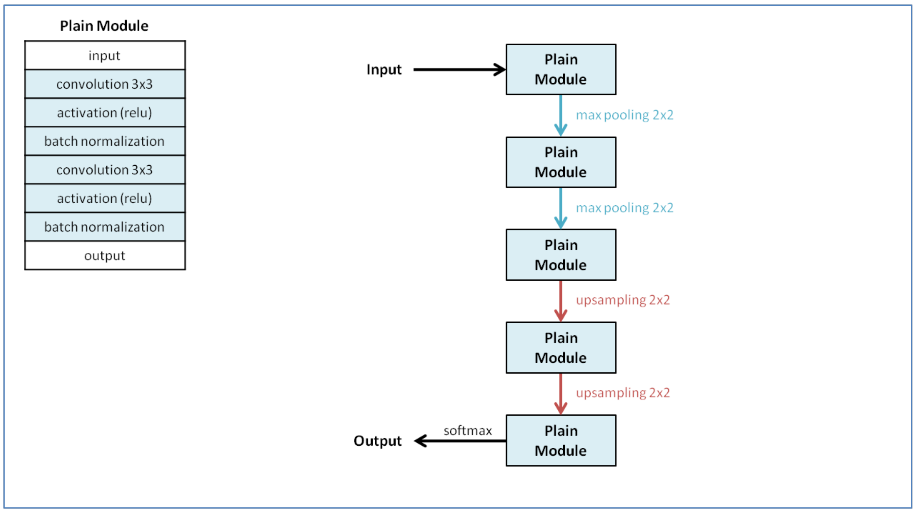
We proposed and evaluated several CNN architectures to study the effect that using different network designs has on performance. The first one is a plain CNN structured in blocks of convolution, activation, and batch normalization layers. We have found that placing each batch normalization layer after the corresponding activation layer provides a slight performance improvement over placing them before, as stated in the original proposal [41].
Our plain model follows an encoder–decoder pattern. The encoder section uses max pooling to reduce the image dimensions, capturing context, and the decoder section reverts the image to its original size through upsampling, enabling feature localization. Our plain model is analogous to the one proposed by Franz et al. [26] but adapted to distinguish between cyclonic and anticyclonic eddies. We experimented with numerous alternatives for this architecture and found that the more max pooling and upsampling layers we added, the harder the CNN became to optimize. Consequently, we reduced the number of these layers and regrouped the others. The best version of our plain model, shown in Figure 3, has 21,248 trainable parameters, just 10% less than the architecture proposed by Franz et al.
The U-net architecture [28] makes it possible to optimize deeper networks through the implementation of a more advanced encoder–decoder pattern. This architecture introduces links between the encoding and decoding stages, allowing the decoding stage to combine the available information with high resolution features provided by the encoding stage, thereby generating more precise outputs. As an additional benefit, the propagation of information from the initial layers to the later ones helps to train deeper networks.
We tested numerous variants of our U-net model and verified that this design is able to successfully train deeper networks than the plain model allows. However, beyond a certain depth, the performance improvements were negligible. The best version of our U-net neural network, shown in Figure 4, has 25,856 trainable parameters, which is 22% more than our plain model. Overall, our U-net model is analogous to the EddyNet architecture [27] proposed by Lguensat et al. Nevertheless, our model has a max pooling level less than EddyNet, which implies a 31% reduction in the total number of trainable parameters.
The low number of max pooling layers used by the best version of our U-net network illustrates an essential difference between the detection of eddies and the typical real-life scene parsing scenario. The objective of max pooling layers is to reduce the image resolution such that the model learns to detect the general structure of objects, omitting an excessive level of detail that would not provide useful information. In this case, the structure of an eddy in satellite imagery is simpler than the structure of the objects frequently found by the CNN models used for computer vision. As a consequence, excessively reducing the resolution of the image is not a benefit; actually we have found that it can even harm the performance of the model.
Residual architectures [30] make it possible to train even deeper neural networks. These architectures reorganize the convolution layers to directly fit a residual mapping with reference to the input layers. A residual neural network follows an encoder–decoder pattern in the same way that the U-net architecture does, setting links between the encoding and decoding stages that provide the model representation with its characteristic u-shape. The main difference from other alternatives is that the residual design introduces feedback points within each stage, which allow the model to revisit information from previous layers.
We tested several alternatives proposed in the literature for the design of our residual model [29,42,43] and subsequently concluded in the elaboration of our own mapping, shown in Figure 5. As with previous models, we found that the best performance was obtained by only applying max pooling twice. However, this more advanced design allows the inclusion of further layers between two levels of max pooling, significantly increasing the model size with respect to the rest of our models. Our residual model has 50,752 trainable parameters, 139% more than our plain model and 96% more than our U-net model. The number of trainable parameters of our residual model is very close to the number of parameters of the EddyResNet architecture [29] proposed by Lguensat et al, under 1% less, although the layer organization of both architectures is significantly different.
3. Results
Understanding the behavior of a CNN requires more than just inspecting its evaluation results; it requires examining all the elements involved in the training and testing processes. Therefore, we begin by analyzing the features of the satellite altimetry images and the segmentation masks used to classify the pixels of these images. Next, we present the evaluation results obtained using the two metrics under study: accuracy and the Sørensen–Dice coefficient.
3.1. Satellite Altimetry Data
To illustrate the differences between the SSH input data and the SLA input data, Figure 6 shows the first day of our test dataset: 1st January 2011. These figures allow one to visually verify that the altimetry values are more widely spread in the case of the SSH data than in the case of the SLA data.
Figure 7 shows the variation of the average altimetry value for each day in our datasets, and the minimum and maximum values. There are a total of 4383 days, 4018 for the training dataset and 365 for the testing dataset. The mean value does not show a great difference between both data sources. Overall, the mean value of the SSH data is 0.053, while the mean value of the SLA data is 0.031.
The key difference between the two data sets, however, is the standard deviation. Dashed lines in Figure 7 plot the evolution of the standard deviation for each day in our datasets. Clearly, the standard deviation is much higher for the SSH data than for the SLA data. The value of the standard deviation for the entire SSH data series is 0.589, but it is just 0.086 for the SLA data series; that is, the SLA standard deviation is an order of magnitude lower than the SSH standard deviation.
3.2. Eddy Segmentation Masks
The images of the satellite altimetry dataset were segmented by assigning each pixel to one of three categories: cyclonic eddies, anticyclonic eddies and background. The latter category includes any pixel that does not belong to an eddy, whether it is part of the ocean or land. We have found that dividing the background pixels in those two separate categories does not provide any significant variation in CNN performance.
Figure 8 shows the segmentation masks for the first day of our test dataset, 1st January 2011, thereby facilitating a visual comparison with the altimetry data for the same day shown in Figure 6. It became clear that there is a huge difference between the two algorithms: OpenEddy identifies substantially more pixels as belonging to an eddy than py-eddy-tracker.
Table 1 shows the percentage of pixels for each category. These percentages were calculated from the complete set of images corresponding to the 12 years covered by our study. The py-eddy-tracker algorithm barely identified 9% of the pixels as eddies, while the OpenEddy algorithm identified as eddies over 31% of the pixels. Another relevant aspect is that the OpenEddy algorithm identified a similar amount of pixels as cyclonic and anticyclonic eddies, whereas the py-eddy-tracker algorithm identified about 70% more anticyclonic eddies than cyclonic ones.
It would be interesting to analyze the reasons for these discrepancies. Both algorithms are based on similar geometrical principles, although they were applied to different input data: py-eddy-tracker to SSH images and OpenEddy to SLA images. Further research is required to determine whether the causes of these substantial differences lay in the input data or in the algorithms themselves, but this topic goes beyond the scope of this paper.
3.3. Evaluation Results
Since the three classes in our segmentation datasets were greatly unbalanced, we trained our CNN models to maximize a weighted average of the Sørensen–Dice coefficient. To ensure balance, each class was given a weight that was inversely proportional to its frequency of occurrence. We had two different segmentation datasets, which means that we needed to train two different versions of each CNN architecture using different weights, one to classify eddies according to the py-eddy-tracker algorithm and another to classify them according to the OpenEddy algorithm. As we also had two different image datasets, SSH and SLA images, we generated a total of four different variants for each CNN model.
Table 2 shows the accuracies of our three CNN models for each of the four possible dataset combinations. According to these results, all the models would provide excellent performance and the dataset selection would make very little difference. However, these data are misleading, since, as previously discussed, accuracy is not an appropriate metric in this context.
For example, the plain model provided an accuracy of 0.967 when identifying cyclonic eddies using SSH images and the py-eddy-tracker segmentation masks. This value did not allow us to know whether the model was correctly identifying cyclonic eddies, since it was calculated by merging the identification of pixels that corresponded to cyclonic eddies, which was what we are interested in, with the identification of pixels that did not correspond to cyclonic eddies, mostly background pixels.
Table 3 shows the value of the Sørensen–Dice coefficient corresponding to our three CNN models for each of the four possible dataset combinations. Completely different conclusions can be drawn from the study of these values. All CNN variants provide excellent performance when identifying background pixels. In contrast, eddy identification performance varies greatly between the different CNN alternatives.
These results prove that the high performances of CNN architectures identifying background pixels distorted the accuracy values, invalidating accuracy as a metric to evaluate the performance of CNN models designed to identify and classify eddies. Going back to the previous example, the plain model provided a Sørensen–Dice coefficient value of just 0.534 for cyclonic eddies. This means that, although the accuracy of the CNN was really high for cyclonic eddies, it actually was only able to correctly identify half of the cyclonic eddies. In contrast, the Sørensen–Dice coefficient value was 0.952 for background pixels, which demonstrates that this particular model is very good at identifying non-eddy pixels, but makes unacceptable errors identifying eddy pixels. Therefore, to ensure a fair comparison, the analysis of the different CNN models and the respective dataset combinations must be done on the basis of the Sørensen–Dice coefficient values shown in Table 3.
3.4. Model Analysis
Using SLA images involves a performance improvement compared to using SSH images, since they have a lower standard deviation and thus favor the CNN learning process. This improvement is significant regardless the CNN architecture and the algorithm used for image segmentation. The increase in the value of the Sørensen–Dice coefficient achieved using SLA images was between 13.3% and 16.7% when using the py-eddy-tracker algorithm, and between 23.2% and 25.8% when using the OpenEddy algorithm.
These results show that, although training a CNN via use of SSH or SLA is valid for eddy structure identification, the use of SLA leads to a more precise structure detection and provides a better classification performance. The benefit in training a CNN with SLA comes from the fact that distinct eddy features are directly correlated to SLA, since eddies physically create a sea level anomaly. Extracting these eddy features is also possible from raw SSH, but doing so basically involves computing the SLA.
Using the OpenEddy algorithm leads to even greater performance improvements when compared to using the py-eddy-tracker algorithm. Once again, this improvement is substantial regardless of the CNN architecture and the image dataset choice. The increase in the value of the Sørensen–Dice coefficient achieved using the OpenEddy algorithm was between 22.9% and 32.9% when working with SSH images, and between 34.6% and 41.5% when working with SLA images.
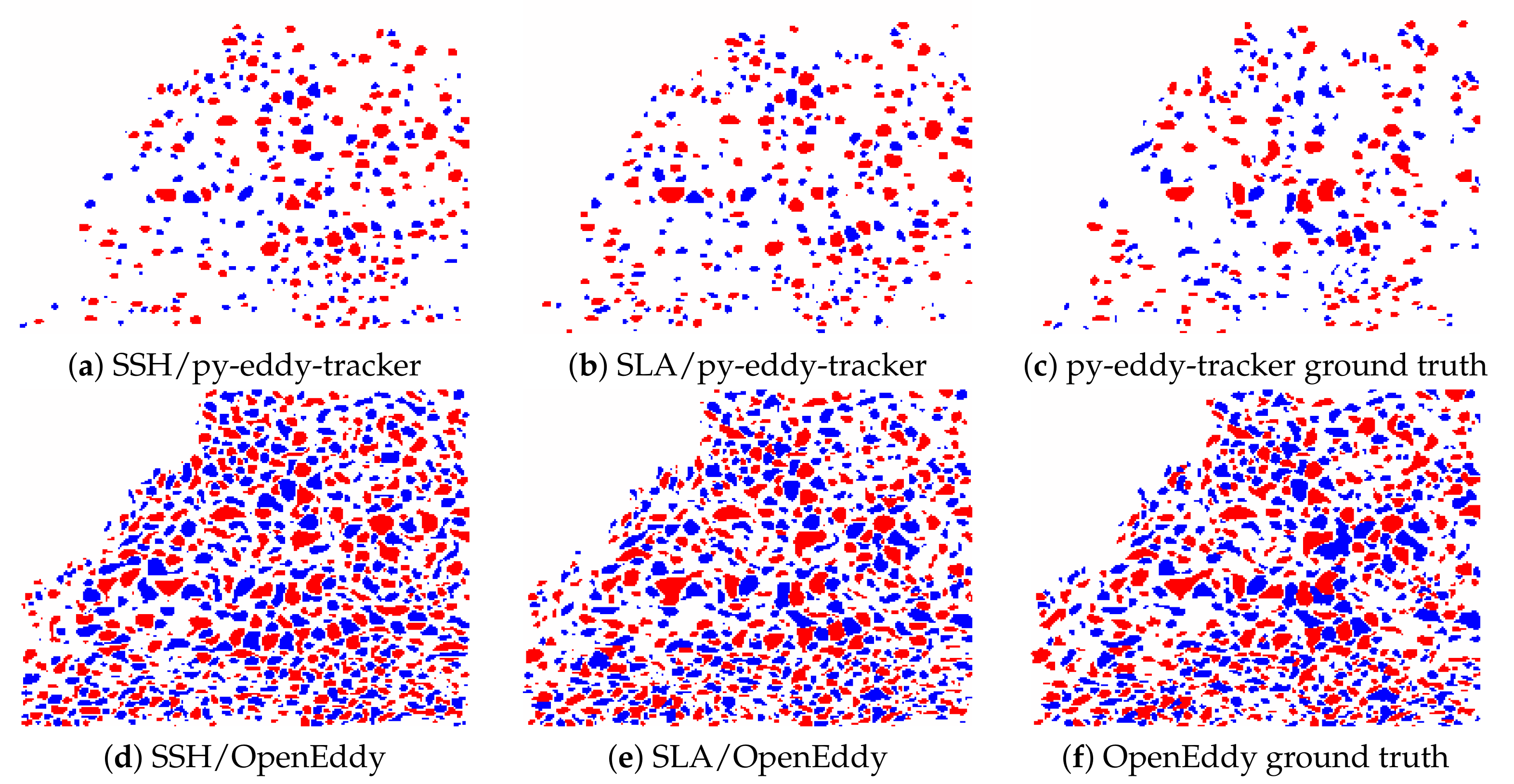
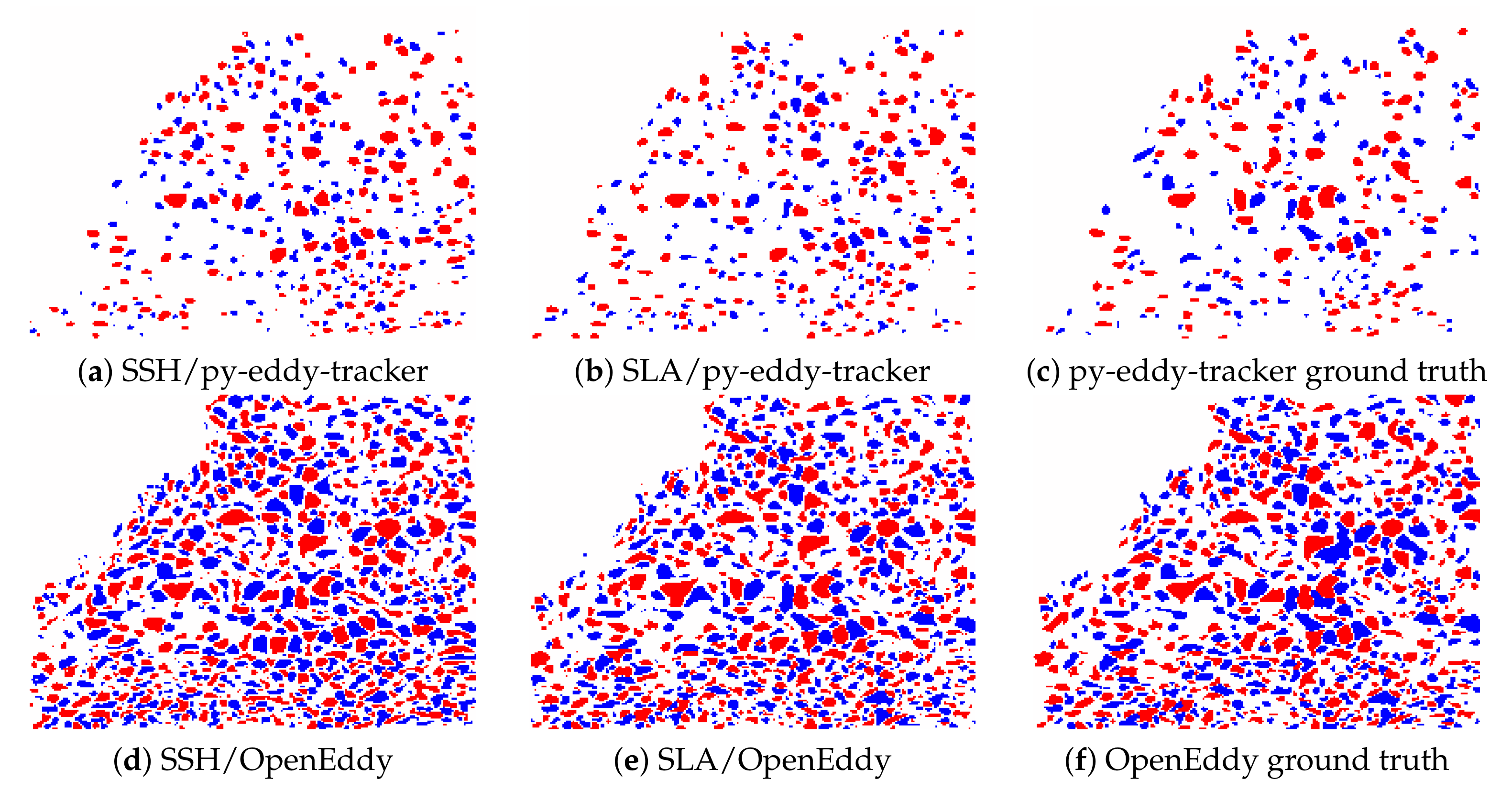
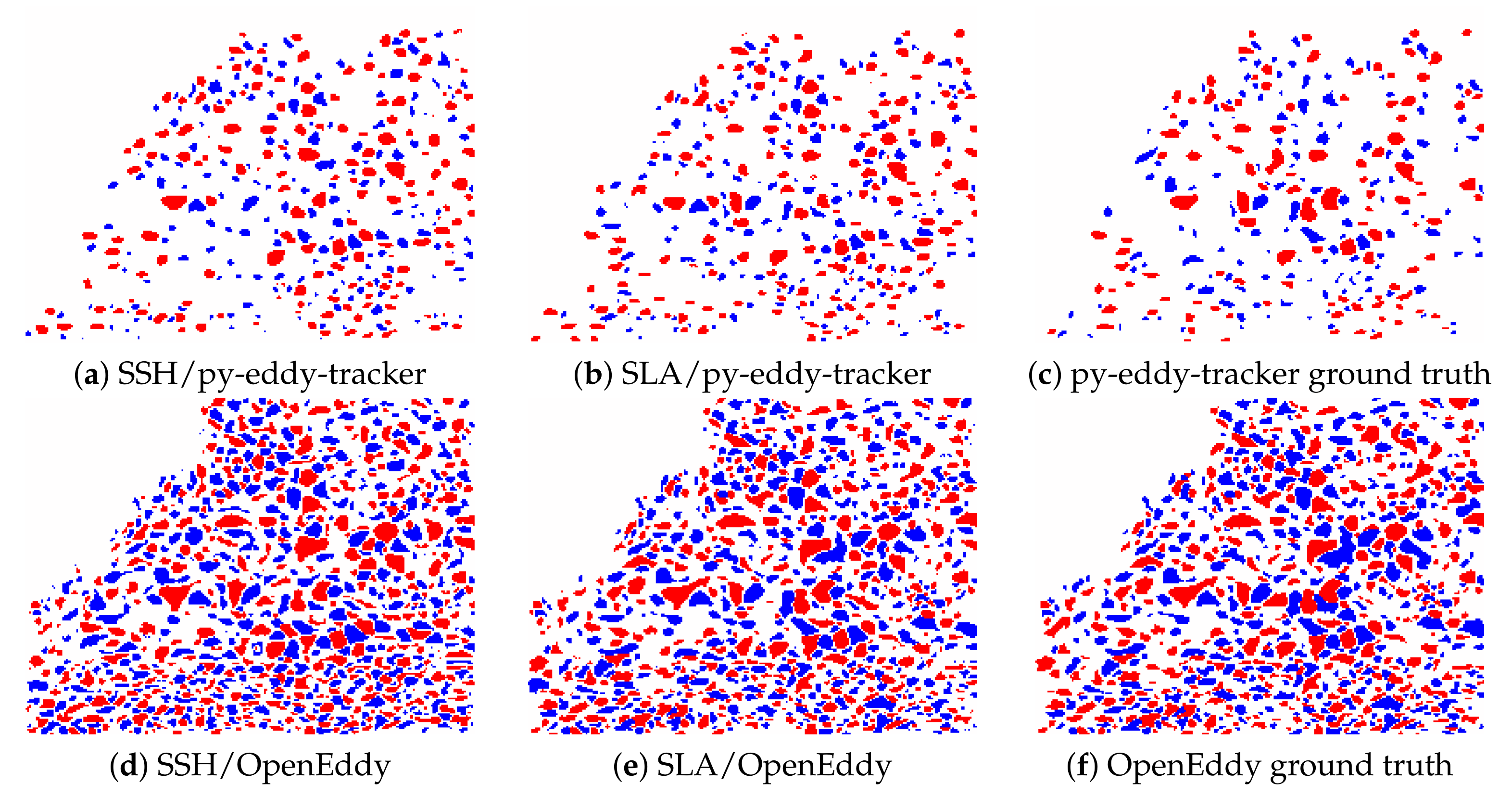
Appendix A shows the eddy segmentation masks generated by our CNN models for 1st January 2011. Cyclonic eddies are shown in blue and anticyclonic eddies are shown in red. The figures provided in this appendix make it possible to visually confirm that the segmentation generated by each CNN model from SLA images was always closer to the corresponding ground truth than the segmentation generated from SSH images. In the same way, the segmentation generated by each CNN model using the OpenEddy algorithm was closer to the OpenEddy ground truth than the segmentation generated using the py-eddy-tracker algorithm was to the py-eddy-tracker ground truth.
The main reason for the OpenEddy algorithm yielding better results than the py-eddy-tracker algorithm is that the former detects a higher number of eddies, and therefore, it increases the amount of information available for CNN training. Table 4 shows the number of epochs the training process of each model had to iterate through before converging to the optimal value. These data clearly show that the models using the OpenEddy algorithm require many more epochs to reach the optimal value, since they have to process more information. The use of SLA images also involves an increase in the number of epochs required, as the closer relationship between the eddy features and the SLA data allows CNN architectures to create more accurate models.
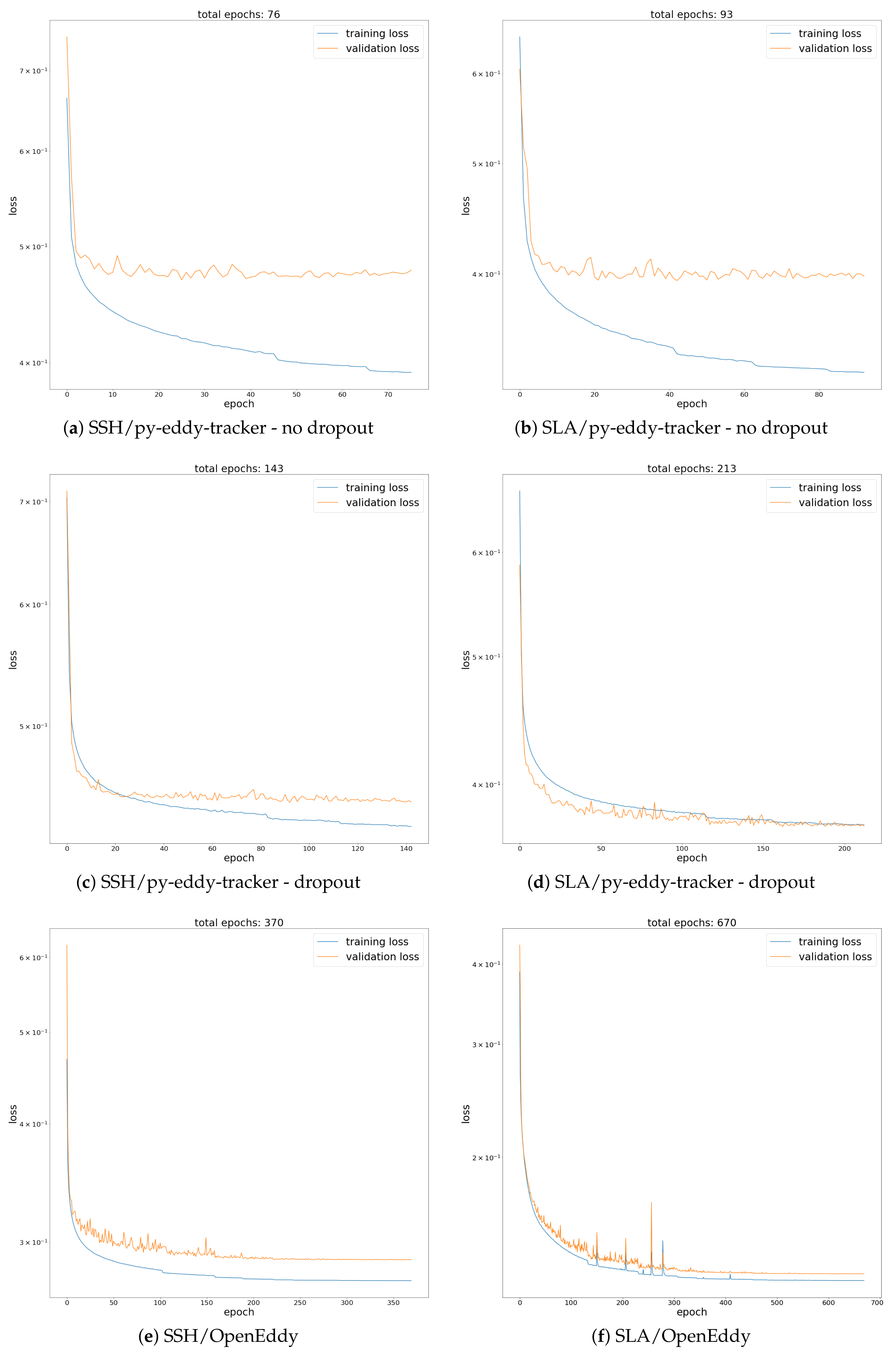
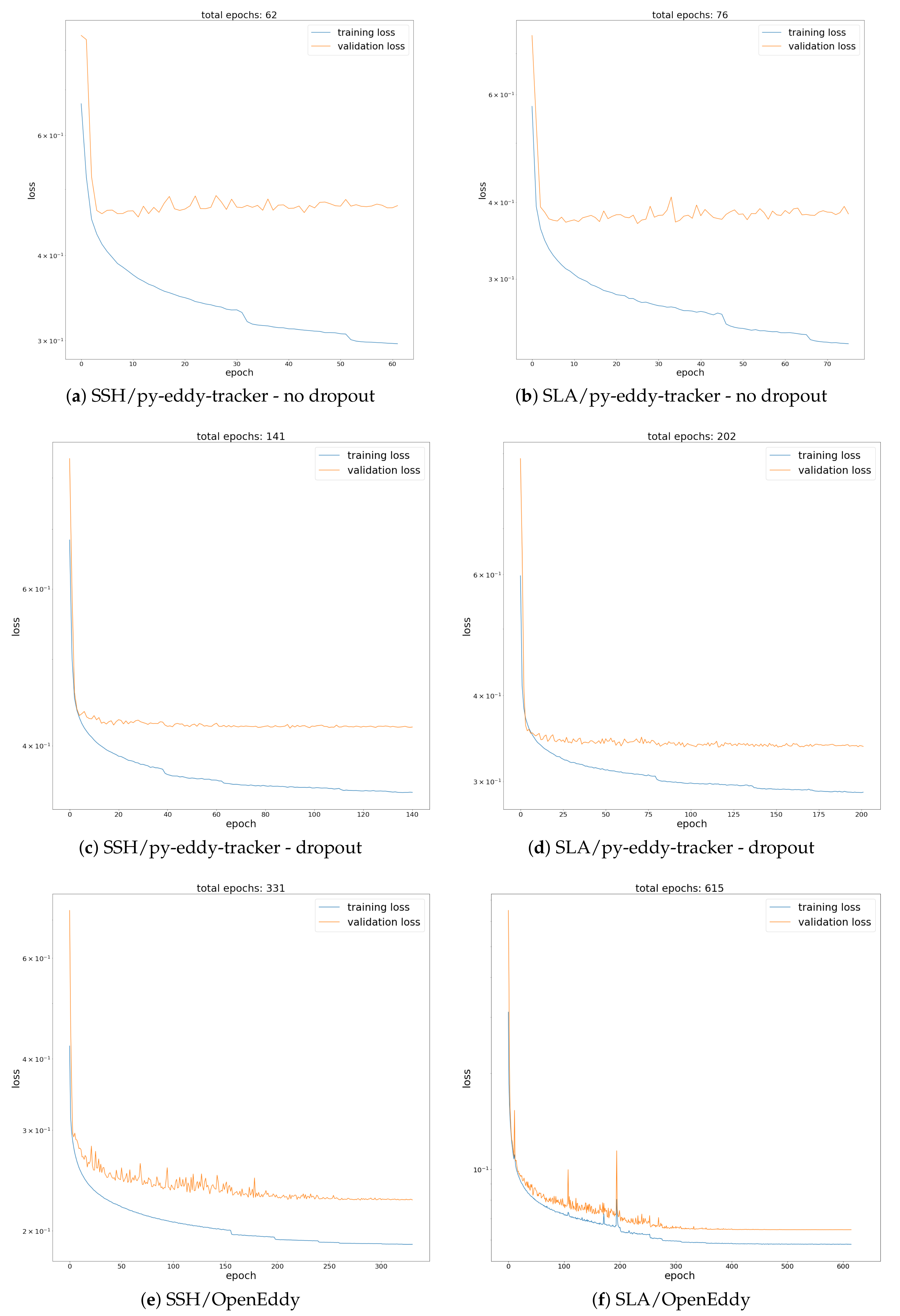
Appendix B shows the learning curves of the training process for our three CNN models. The training loss curve of the models trained using the OpenEddy algorithm are similar to their corresponding validation loss curves, which means that the models have the ability to generalize the learned knowledge well. In contrast, the training loss curves of the models trained using the py-eddy-tracker algorithm differ significantly from their corresponding validation loss curves, which is a clear sign of overfitting: the learned models do not generalize well for datasets other than the training one.
To solve this problem, we added a dropout layer [44] behind every activation layer of the CNN models trained using the py-eddy-tracker segmentation masks. The CNN models trained using the OpenEddy segmentation data did not include dropout layers because we found no performance benefit from doing so. These dropout layers were configured to randomly select and deactivate 5% of the neurons during each epoch of the training process, preventing overfitting.
For illustration purposes, Appendix B shows two versions of the learning curves for the models using the py-eddy-tracker algorithm: with and without dropout. These figures clearly show that the models using the py-eddy-tracker algorithm without dropout converged quickly in a few epochs to an overfitted value that could not be generalized later for the validation dataset. Using dropout adjusts this behavior, allowing the loss curves of the py-eddy-tracker algorithm to be much closer to those of the OpenEddy algorithm.
4. Discussion
Our results demonstrate the importance of properly choosing the right data for CNN training. As shown in Table 3, the best performance was obtained by combining the SLA images with the segmentation generated by the OpenEddy algorithm. Once the appropriate data are chosen, increasing the complexity of the CNN model is not as beneficial. This is a natural consequence, given that the results are closer to the maximum value.
Using the SLA images and the OpenEddy segmentation masks, our U-net model improved the detection of cyclonic eddies by 6.1% and the detection of anticyclonic eddies by 5.8% compared to our plain model. This is a reasonable tradeoff, since our U-net model has only 22% more trainable parameters than our plain model. The improvement of our residual model over our U-net model was lower: 2.1% for cyclonic eddies and 2.3% for anticyclonic eddies. It should be taken into account that our residual model has almost twice the number of trainable parameters as our U-net model, so the benefit provided by this improvement should be considered in the context of the available resources for CNN training.
Overall, our residual model yielded better performance for eddy detection and classification than any of the previous proposals in the literature. It provided a value of the Sørensen–Dice coefficient of over 0.93 for both cyclonic and anticyclonic eddies, which is significantly higher than the values reported for EddyNet, EddyResNet, and EddyVNet by Lguensat et al. [27,29], who used the same metric, thereby allowing a direct comparison. Franz et al. [26] used precision and recall, metrics directly related to the Sørensen–Dice coefficient, but they did not report the obtained values, so it is not possible to make a well founded comparison; in any case, their CNN model is not able to distinguish between both eddy types.
Although we have shown that accuracy is not an appropriate metric, it permits one to compare our proposals with other works that have only reported values for this metric. The accuracy of our U-net and residual models is really close to the accuracy obtained by DeepEddy for SAR images [25]. In the context of satellite altimetry data, the accuracies of our U-net and residual models are also higher than the values reported by Fan et al. [32] for their symmetrical network. Xu et al. evaluated their PSPNet model [34] using the number of detected eddies as a metric. This hampers the model assessment because it does not allow one to distinguish whether the detected eddies are real or not. On the other hand, Fan et al. [32] also evaluated PSPNet and reported accuracy data, which makes it possible to verify that our U-net and residual models also provide better results than PSPNet.
5. Conclusions
Ocean mesoscale eddies are the terrestrial weather analog to the ocean. However, for all we know about the impacts of eddies, their formation, evolution and eventual dissipation are still poorly understood. To this end, the research in this paper aims to provide tools that facilitate the characterization of eddy dynamics, both spatially and temporally, and to deepen our understanding of these and other ocean processes.
This is the first comparative study that used both SSH and SLA images to train CNN architectures and reports the consequences of choosing one or another. According to our results, using SLA data is widely preferable and leads to CNN models with far better performances. Our results also show that accuracy is a misleading metric for eddy detection and classification, as its value is distorted because CNN models detect non-eddy pixels easily. Therefore, it is more appropriate to use the Sørensen–Dice coefficient, a metric equivalent to the F1 score which combines precision and recall.
Based on these principles, we have proposed and evaluated three CNN architectures, proving that the most advanced models allow for the training of deeper networks, yielding better performance. Furthermore, our two most elaborate models performed better than any of the previously proposed CNN models for eddy detection and classification using satellite altimetry data.
Nevertheless, while more advanced architectures may provide better performance, our results demonstrate that most of the gain comes from choosing the appropriate input data. This conclusion points out that the most promising line of research in this field is to develop an adequate treatment of the available data instead of proposing the implementation of increasingly complex and expensive CNN architectures. In this sense, it would be of great interest to evaluate the impact of feeding CNN models not only with SLA data but also with useful complementary data for eddy characterization, such as geostrophic currents, water temperature and salinity levels.
Author Contributions
Conceptualization, O.J.S., D.H.-S. and R.N.S.; data curation, O.J.S. and D.H.-S.; formal analysis, O.J.S., D.H.-S., J.M. and R.N.S.; funding acquisition, D.H.-S., J.M. and R.N.S.; investigation, O.J.S. and D.H.-S.; methodology, O.J.S. and D.H.-S.; project administration, O.J.S. and D.H.-S.; resources, O.J.S. and D.H.-S.; software, O.J.S. and D.H.-S.; supervision, O.J.S. and D.H.-S.; validation, O.J.S. and D.H.-S.; visualization, O.J.S.; writing—original draft, O.J.S.; writing—review and editing, O.J.S., D.H.-S., J.M. and R.N.S. All authors have read and agreed to the published version of the manuscript.
Funding
This research was funded in part by the US Office of Naval Research Award N00014161263, the SIANI research institute and ESF cooperation project CZ.02.2.69/0.0/0.0/16_015/0002204.
Acknowledgments
The authors would like to thank James H. Faghmous for releasing the OpenEddy segmentation masks and Redouane Lguensat for releasing the py-eddy-tracker segmentation masks.
Conflicts of Interest
The authors declare no conflict of interest.
Appendix A. Segmentation Masks Generated by Our CNN Models for 1 January 2011
Figure A1.
Plain model.

Figure A2.
U-net model.

Figure A3.
Residual model.

Appendix B. Learning Curves Obtained during the Training Process of Our CNN Models
Figure A4.
Learning curves for our plain CNN model. The x-axis shows the number of optimization process epochs and the y-axis shows the loss function value. The blue line represents the training dataset and the orange line represents the validation dataset.
Figure A4.
Learning curves for our plain CNN model. The x-axis shows the number of optimization process epochs and the y-axis shows the loss function value. The blue line represents the training dataset and the orange line represents the validation dataset.

Figure A5.
Learning curves for our U-net CNN model. The x-axis shows the number of optimization process epochs and the y-axis shows the loss function value. The blue line represents the training dataset and the orange line represents the validation dataset.
Figure A5.
Learning curves for our U-net CNN model. The x-axis shows the number of optimization process epochs and the y-axis shows the loss function value. The blue line represents the training dataset and the orange line represents the validation dataset.

Figure A6.
Learning curves for our residual CNN model. The x-axis shows the number of optimization process epochs and the y-axis shows the loss function value. The blue line represents the training dataset and the orange line represents the validation dataset.
Figure A6.
Learning curves for our residual CNN model. The x-axis shows the number of optimization process epochs and the y-axis shows the loss function value. The blue line represents the training dataset and the orange line represents the validation dataset.

References
- Morrow, R.; Le Traon, P.Y. Recent advances in observing mesoscale ocean dynamics with satellite altimetry. Adv. Space Res. 2012, 50, 1062–1076. [Google Scholar] [CrossRef] [Green Version]
- Mcwilliams, J.C. The nature and consequences of oceanic eddies. In Ocean Modeling in an Eddying Regime; American Geophysical Union (AGU): Washington, DC, USA, 2013; pp. 5–15. [Google Scholar] [CrossRef] [Green Version]
- Falkowski, P.G.; Ziemann, D.; Kolber, Z.; Bienfang, P.K. Role of eddy pumping in enhancing primary production in the ocean. Nature 1991, 352, 55–58. [Google Scholar] [CrossRef]
- Ji, J.; Ma, J.; Dong, C.; Chiang, J.; Chen, D. Regional dependence of atmospheric responses to oceanic eddies in the North Pacific Ocean. Remote Sens. 2020, 12, 1161. [Google Scholar] [CrossRef] [Green Version]
- Cheng, Y.; Ho, C.; Zheng, Q.; Kuo, N. Statistical characteristics of mesoscale eddies in the North Pacific derived from satellite altimetry. Remote Sens. 2014, 6, 5164–5183. [Google Scholar] [CrossRef] [Green Version]
- Sangrá, P.; Pascual, A.; Rodríguez-Santana, A.; Machín, F.; Mason, E.; McWilliams, J.; Pelegrí, J.; Dong, C.; Rubio, A.; Arístegui, J.; et al. The Canary eddy corridor: A major pathway for long-lived eddies in the subtropical North Atlantic. Deep Sea Res. Part I Oceanogr. Res. Pap. 2009, 56, 2100–2114. [Google Scholar] [CrossRef]
- Faghmous, J.H.; Frenger, I.; Yao, Y.; Warmka, R.; Lindell, A.; Kumar, V. A daily global mesoscale ocean eddy dataset from satellite altimetry. Sci. Data 2015, 2, 150028. [Google Scholar] [CrossRef] [Green Version]
- Okubo, A. Horizontal dispersion of floatable particles in the vicinity of velocity singularities such as convergences. Deep Sea Res. Oceanogr. Abstr. 1970, 17, 445–454. [Google Scholar] [CrossRef]
- Weiss, J. The dynamics of enstrophy transfer in two-dimensional hydrodynamics. Phys. D Nonlinear Phenom. 1991, 48, 273–294. [Google Scholar] [CrossRef]
- Chelton, D.B.; Schlax, M.G.; Samelson, R.M. Global observations of nonlinear mesoscale eddies. Prog. Oceanogr. 2011, 91, 167–216. [Google Scholar] [CrossRef]
- Nencioli, F.; Dong, C.; Dickey, T.; Washburn, L.; McWilliams, J.C. A vector geometry–based eddy detection algorithm and its application to a high-resolution numerical model product and high-frequency radar surface velocities in the Southern California Bight. J. Atmos. Ocean. Technol. 2010, 27, 564–579. [Google Scholar] [CrossRef]
- Mason, E.; Pascual, A.; McWilliams, J.C. A new sea surface height–based code for oceanic mesoscale eddy tracking. J. Atmos. Ocean. Technol. 2014, 31, 1181–1188. [Google Scholar] [CrossRef] [Green Version]
- Schlax, M.G.; Chelton, D. The “Growing Method” of Eddy Identification and Tracking in Two and Three Dimensions; College of Earth, Ocean and Atmospheric Sciences, Oregon State University: Corvallis, OR, USA, 2016. [Google Scholar]
- Zhang, Y.; Godin, M.A.; Bellingham, J.G.; Ryan, J.P. Using an Autonomous Underwater Vehicle to Track a Coastal Upwelling Front. IEEE J. Ocean. Eng. 2012, 37, 338–347. [Google Scholar] [CrossRef]
- Caron, D.A.; Stauffer, B.; Moorthi, S.; Singh, A.; Batalin, M.; Graham, E.; Hansen, M.; Kaiser, W.; Das, J.; Pereira, A.A.; et al. Macro- to fine-scale spatial and temporal distributions and dynamics of phytoplankton and their environmental driving forces in a small subalpine lake in southern California, USA. J. Limnol. Oceanogr. 2008, 53, 2333–2349. [Google Scholar] [CrossRef] [Green Version]
- Wu, W.; Zhang, F. Cooperative exploration of level surfaces of three dimensional scalar fields. Automatica 2011, 47, 2044–2051. [Google Scholar] [CrossRef]
- Smith, R.N.; Chao, Y.; Li, P.P.; Caron, D.A.; Jones, B.H.; Sukhatme, G.S. Planning and Implementing Trajectories for Autonomous Underwater Vehicles to Track Evolving Ocean Processes based on Predictions from a Regional Ocean Model. Int. J. Robot. Res. 2010, 29, 1475–1497. [Google Scholar] [CrossRef] [Green Version]
- Shaw, A.G.P.; Vennell, R. A Front-Following Algorithm for AVHRR SST imagery. Remote Sens. Environ. 2000, 72, 317–327. [Google Scholar] [CrossRef]
- Hopkins, J.; Challenor, P.; Shaw, A.G.P. A New Statistical Modeling Approach to Ocean Front Detection from SST Satellite Images. J. Atmos. Ocean. Technol. 2010, 27, 173–191. [Google Scholar] [CrossRef] [Green Version]
- Shanmugam, P.; Suresh, M.; Sundarabalan, B. OSABT: An Innovative Algorithm to Detect and Characterize Ocean Surface Algal Blooms. IEEE J. Sel. Top. Appl. Earth Obs. Remote Sens. 2013, 6, 1879–1892. [Google Scholar] [CrossRef]
- Shadden, S.C.; Lekien, F.; Marsden, J.E. Definition and properties of lagrangian coherent structures from finite-time lyapunov exponents in two-dimensional aperiodic flows. Phys. D Nonlinear Phenom. 2005, 212, 271–304. [Google Scholar] [CrossRef]
- Haller, G.; Yuan, G. Lagrangian coherent structures and mixing in two-dimensional turbulence. Phys. D Nonlinear Phenom. 2000, 147, 352–370. [Google Scholar] [CrossRef]
- Zhan, P.; Subramanian, A.C.; Yao, F.; Hoteit, I. Eddies in the Red Sea: A statistical and dynamical study. J. Geophys. Res. (Oceans) 2014, 119, 3909–3925. [Google Scholar] [CrossRef] [Green Version]
- Faghmous, J.H.; Le, M.; Uluyol, M.; Kumar, V.; Chatterjee, S. A Parameter-Free Spatio-Temporal Pattern Mining Model to Catalog Global Ocean Dynamics. In Proceedings of the 2013 IEEE 13th International Conference on Data Mining, Dallas, TX, USA, 7–10 December 2013; pp. 151–160. [Google Scholar] [CrossRef]
- Du, Y.; Song, W.; He, Q.; Huang, D.; Liotta, A.; Su, C. Deep learning with multi-scale feature fusion in remote sensing for automatic oceanic eddy detection. Inf. Fusion 2019, 49, 89–99. [Google Scholar] [CrossRef] [Green Version]
- Franz, K.; Roscher, R.; Milioto, A.; Wenzel, S.; Kusche, J. Ocean eddy identification and tracking using neural networks. In Proceedings of the IGARSS 2018—2018 IEEE International Geoscience and Remote Sensing Symposium, Valencia, Spain, 22–27 July 2018; pp. 6887–6890. [Google Scholar] [CrossRef] [Green Version]
- Lguensat, R.; Sun, M.; Fablet, R.; Tandeo, P.; Mason, E.; Chen, G. EddyNet: A deep neural network for pixel-wise classification of oceanic eddies. In Proceedings of the IGARSS 2018—2018 IEEE International Geoscience and Remote Sensing Symposium, Valencia, Spain, 22–27 July 2018; pp. 1764–1767. [Google Scholar] [CrossRef] [Green Version]
- Ronneberger, O.; Fischer, P.; Brox, T. U-Net: Convolutional networks for biomedical image segmentation. In Medical Image Computing and Computer-Assisted Intervention—MICCAI 2015, Proceedings of the 18th International Conference, Munich, Germany, 5–9 October 2015; Navab, N., Hornegger, J., Wells, W.M., Frangi, A.F., Eds.; Springer International Publishing: Cham, Switzerland, 2015; pp. 234–241. [Google Scholar] [CrossRef] [Green Version]
- Lguensat, R.; Rjiba, S.; Mason, E.; Fablet, R.; Sommer, J. Convolutional neural networks for the segmentation of oceanic eddies from altimetric maps. Remote Sens. 2018. [Google Scholar] [CrossRef]
- He, K.; Zhang, X.; Ren, S.; Sun, J. Deep residual learning for image recognition. In Proceedings of the 2016 IEEE Conference on Computer Vision and Pattern Recognition (CVPR), Las Vegas, NV, USA, 27–30 June 2016; pp. 770–778. [Google Scholar] [CrossRef] [Green Version]
- Milletari, F.; Navab, N.; Ahmadi, S. V-Net: Fully convolutional neural networks for volumetric medical image segmentation. In Proceedings of the 2016 Fourth International Conference on 3D Vision (3DV), Stanford, CA, USA, 25–28 October 2016; pp. 565–571. [Google Scholar] [CrossRef] [Green Version]
- Fan, Z.; Zhong, G. SymmetricNet: A mesoscale eddy detection method based on multivariate fusion data. arXiv 2019, arXiv:cs.CV/1909.13411. [Google Scholar]
- Yu, F.; Koltun, V. Multi-scale context aggregation by dilated convolutions. In Proceedings of the International Conference on Learning Representations (ICLR), San Juan, Puerto Rico, 2–4 May 2016. arXiv:cs.CV/1511.07122. [Google Scholar]
- Xu, G.; Cheng, C.; Yang, W.; Xie, W.; Kong, L.; Hang, R.; Ma, F.; Dong, C.; Yang, J. Oceanic eddy identification using an AI scheme. Remote Sens. 2019, 11, 1349. [Google Scholar] [CrossRef] [Green Version]
- Zhao, H.; Shi, J.; Qi, X.; Wang, X.; Jia, J. Pyramid scene parsing network. In Proceedings of the 2017 IEEE Conference on Computer Vision and Pattern Recognition (CVPR), Honolulu, HI, USA, 21–26 July 2017; pp. 6230–6239. [Google Scholar] [CrossRef] [Green Version]
- Kingma, D.P.; Ba, J. Adam: A method for stochastic optimization. In Proceedings of the 3rd International Conference for Learning Representations, San Diego, CA, USA, 7–9 May 2015. [Google Scholar]
- He, K.; Zhang, X.; Ren, S.; Sun, J. Delving deep into rectifiers: Surpassing human-level performance on ImageNet classification. In Proceedings of the 2015 IEEE International Conference on Computer Vision (ICCV), Santiago, Chile, 7–13 December 2015; pp. 1026–1034. [Google Scholar] [CrossRef] [Green Version]
- Sørensen, T. A method of establishing groups of equal amplitude in plant sociology based on similarity of species and its application to analyses of the vegetation on Danish commons. K. Dan. Vidensk. Selsk. 1948, 5, 1–34. [Google Scholar]
- Dice, L. Measures of the amount of ecologic association between species. Ecology 1945, 29, 297–302. [Google Scholar] [CrossRef]
- Chinchor, N. MUC-4 evaluation metrics. In Proceedings of the 4th Conference on Message Understanding (MUC4’92), McLean, VA, USA, 16–18 June 1992; pp. 22–29. [Google Scholar] [CrossRef] [Green Version]
- Ioffe, S.; Szegedy, C. Batch Normalization: Accelerating Deep Network Training by Reducing internal Covariate Shift. In Proceedings of the 32nd International Conference on International Conference on Machine Learning, Lille, France, 7–9 July 2015; Volume 37, pp. 448–456. [Google Scholar] [CrossRef]
- He, K.; Zhang, X.; Ren, S.; Sun, J. Identity mappings in Deep Residual Networks. In Computer Vision—ECCV 2016, Proceedings of the 14th European Conference, Amsterdam, The Netherlands, 11–14 October 2016; Leibe, B., Matas, J., Sebe, N., Welling, M., Eds.; Springer International Publishing: Cham, Switzerland, 2016; pp. 630–645. [Google Scholar] [CrossRef] [Green Version]
- Zhang, Z.; Liu, Q.; Wang, Y. Road extraction by deep residual U-net. IEEE Geosci. Remote Sens. Lett. 2018, 15, 749–753. [Google Scholar] [CrossRef] [Green Version]
- Srivastava, N.; Hinton, G.; Krizhevsky, A.; Sutskever, I.; Salakhutdinov, R. Dropout: A simple way to prevent neural networks from overfitting. J. Mach. Learn. Res. 2014, 15, 1929–1958. [Google Scholar]
Figure 1.
Processing pipeline for the CNN architectures proposed in this article.

Figure 2.
Region of the Southern Atlantic Ocean corresponding to our satellite altimetry data.

Figure 3.
Architectural design of our plain CNN model.

Figure 4.
Architectural design of our U-net CNN model.

Figure 5.
Architectural design of our residual CNN model.

Figure 6.
Satellite altimetry data for 1st January 2011.

Figure 7.
Mean, minimum and maximum satellite altimetry values on each day of the 12 years covered. The standard deviation is marked along the mean using dashed lines.
Figure 7.
Mean, minimum and maximum satellite altimetry values on each day of the 12 years covered. The standard deviation is marked along the mean using dashed lines.

Figure 8.
Eddy segmentation masks for 1st January 2011. Cyclonic eddies are shown in blue and anticyclonic eddies are shown in red.
Figure 8.
Eddy segmentation masks for 1st January 2011. Cyclonic eddies are shown in blue and anticyclonic eddies are shown in red.


Table 1.
Percentage of pixels per category in the whole datasets.
| py-eddy-tracker | OpenEddy | |
|---|---|---|
| background | 91.118% | 68.738% |
| cyclonic eddy | 3.288% | 15.506% |
| anticyclonic eddy | 5.594% | 15.756% |
Table 2.
Accuracy for our three CNN models using the four different dataset combinations. Results are shown separately for each of the three classes under study: background pixels (bgd), cyclonic eddy pixels (cyc) and anticyclonic eddy pixels (ant).
Table 2.
Accuracy for our three CNN models using the four different dataset combinations. Results are shown separately for each of the three classes under study: background pixels (bgd), cyclonic eddy pixels (cyc) and anticyclonic eddy pixels (ant).
| Plain Model | U-Net Model | Residual Model | |||||||||
|---|---|---|---|---|---|---|---|---|---|---|---|
| SSH | SSH | SSH | SSH | SSH | SSH | ||||||
| py-eddy-tracker | OpenEddy | py-eddy-tracker | OpenEddy | py-eddy-tracker | OpenEddy | ||||||
| bgd: | 0.914 | bgd: | 0.801 | bgd: | 0.915 | bgd: | 0.821 | bgd: | 0.916 | bgd: | 0.842 |
| cyc: | 0.967 | cyc: | 0.901 | cyc: | 0.967 | cyc: | 0.911 | cyc: | 0.967 | cyc: | 0.921 |
| ant: | 0.947 | ant: | 0.899 | ant: | 0.948 | ant: | 0.910 | ant: | 0.949 | ant: | 0.921 |
| SLA | SLA | SLA | SLA | SLA | SLA | ||||||
| py-eddy-tracker | OpenEddy | py-eddy-tracker | OpenEddy | py-eddy-tracker | OpenEddy | ||||||
| bgd: | 0.928 | bgd: | 0.911 | bgd: | 0.932 | bgd: | 0.944 | bgd: | 0.933 | bgd: | 0.956 |
| cyc: | 0.972 | cyc: | 0.955 | cyc: | 0.973 | cyc: | 0.972 | cyc: | 0.974 | cyc: | 0.978 |
| ant: | 0.956 | ant: | 0.955 | ant: | 0.958 | ant: | 0.972 | ant: | 0.959 | ant: | 0.978 |
Table 3.
Values of the Sørensen–Dice coefficient for our three CNN models using the four different dataset combinations. Results are shown separately for each of the three classes under study: background pixels (bgd), cyclonic eddy pixels (cyc) and anticyclonic eddy pixels (ant).
Table 3.
Values of the Sørensen–Dice coefficient for our three CNN models using the four different dataset combinations. Results are shown separately for each of the three classes under study: background pixels (bgd), cyclonic eddy pixels (cyc) and anticyclonic eddy pixels (ant).
| Plain Model | U-Net Model | Residual Model | |||||||||
|---|---|---|---|---|---|---|---|---|---|---|---|
| SSH | SSH | SSH | SSH | SSH | SSH | ||||||
| py-eddy-tracker | OpenEddy | py-eddy-tracker | OpenEddy | py-eddy-tracker | OpenEddy | ||||||
| bgd: | 0.952 | bgd: | 0.853 | bgd: | 0.953 | bgd: | 0.867 | bgd: | 0.953 | bgd: | 0.883 |
| cyc: | 0.534 | cyc: | 0.692 | cyc: | 0.558 | cyc: | 0.724 | cyc: | 0.568 | cyc: | 0.755 |
| ant: | 0.564 | ant: | 0.694 | ant: | 0.586 | ant: | 0.726 | ant: | 0.596 | ant: | 0.757 |
| SLA | SLA | SLA | SLA | SLA | SLA | ||||||
| py-eddy-tracker | OpenEddy | py-eddy-tracker | OpenEddy | py-eddy-tracker | OpenEddy | ||||||
| bgd: | 0.960 | bgd: | 0.935 | bgd: | 0.962 | bgd: | 0.959 | bgd: | 0.963 | bgd: | 0.968 |
| cyc: | 0.624 | cyc: | 0.858 | cyc: | 0.643 | cyc: | 0.910 | cyc: | 0.661 | cyc: | 0.930 |
| ant: | 0.640 | ant: | 0.861 | ant: | 0.667 | ant: | 0.911 | ant: | 0.680 | ant: | 0.933 |
Table 4.
Number of epochs required for the training process to converge to the optimal value.
| Plain Model | U-Net Model | Residual Model | |
|---|---|---|---|
| SSH/py-eddy-tracker | 143 | 114 | 141 |
| SLA/py-eddy-tracker | 213 | 166 | 202 |
| SSH/OpenEddy | 370 | 331 | 331 |
| SLA/OpenEddy | 670 | 681 | 615 |
© 2020 by the authors. Licensee MDPI, Basel, Switzerland. This article is an open access article distributed under the terms and conditions of the Creative Commons Attribution (CC BY) license (http://creativecommons.org/licenses/by/4.0/).
Share and Cite
MDPI and ACS Style
Santana, O.J.; Hernández-Sosa, D.; Martz, J.; Smith, R.N. Neural Network Training for the Detection and Classification of Oceanic Mesoscale Eddies. Remote Sens. 2020, 12, 2625. https://0-doi-org.brum.beds.ac.uk/10.3390/rs12162625
AMA Style
Santana OJ, Hernández-Sosa D, Martz J, Smith RN. Neural Network Training for the Detection and Classification of Oceanic Mesoscale Eddies. Remote Sensing. 2020; 12(16):2625. https://0-doi-org.brum.beds.ac.uk/10.3390/rs12162625
Chicago/Turabian StyleSantana, Oliverio J., Daniel Hernández-Sosa, Jeffrey Martz, and Ryan N. Smith. 2020. "Neural Network Training for the Detection and Classification of Oceanic Mesoscale Eddies" Remote Sensing 12, no. 16: 2625. https://0-doi-org.brum.beds.ac.uk/10.3390/rs12162625
Note that from the first issue of 2016, this journal uses article numbers instead of page numbers. See further details here.