Mapping Sea Surface Height Using New Concepts of Kinematic GNSS Instruments

Abstract

For over 25 years, satellite altimetry observations have provided invaluable information about sea-level variations, from Global Mean Sea-Level to regional meso-scale variability. However, this information remains difficult to extract in coastal areas, where the proximity to land and complex dynamics create complications that are not sufficiently accounted for in current models. Detailed knowledge of local hydrodynamics, as well as reliable sea-surface height measurements, is required to improve and validate altimetry measurements. New kinematic systems based on Global Navigation Satellite Systems (GNSS) have been developed to map the sea surface height in motion. We demonstrate the capacity of two of these systems, designed to measure the height at a centimetric level: (1) A GNSS floating carpet towed by boat (named CalNaGeo); and (2) a combination of GNSS antenna and acoustic altimeter (named Cyclopée) mounted on an unmanned surface vehicle (USV). We show that, at a fixed point, these instruments provide comparable accuracy to the best available tide gauge systems. When moving at up to 7 knots, the instrument velocity does not affect the sea surface height accuracy, and the two instruments agree at a cm-level.

1. Introduction

Satellite altimetry observations provide invaluable information about sea-level variations at many scales, from regional meso-scale ocean variability to global sea-level rise. Coastal and near-shore observations are key to answering various questions, such as the nature and role of small-scale processes, land/sea interactions, human impact and vulnerability. Obtaining accurate altimetry information in these areas remains a true challenge, as satellite altimeter and radiometer signals can be contaminated by land [1,2]. Calibration/validation activities (hereafter called “cal/val”) are, therefore, essential to characterize the performance of altimetry missions and to ensure a 1 mm/y stability of regional sea-level measurements [3]. Tide gauges are currently the most frequently used instruments to measure relative sea-level variations at the coast and to calibrate satellite data [4]. They provide accurate and high sampling-rate sea-level measurements at a fixed point and are inexpensive and easy to maintain, making them a simple option for cal/val experiments. However, because they are usually grounded at the coast, they are sometimes distant from satellite ground tracks, and their sea-level estimates may be affected by vertical land movements.

When in-situ measurements are not located under satellite tracks, a very good knowledge of local hydrodynamics corrections and fine-scale spatial variations of the geoid is required to link these measurements to the altimetric measurements. The often-sharp variations of the marine geoid (which is close to the local mean sea surface) induce gradients that may bias the comparison between offshore altimetric and coastal observations. Nearshore, the resolution of global geoid models (for example, EGM08 [5]) is insufficient to reliably map those short scale undulations in order to transfer offshore altimetric measurements to onshore in-situ observations. In addition, reliable geoid gradients along and across satellite tracks are needed for high-resolution processing of altimetry data. Furthermore, global ocean tide models do not handle the shallow-water complexity of tides in most coastal areas [6]. For cal/val activities where tide gauges observations may be several kilometers away from satellite tracks, local hydrodynamic models are essential to accurately estimate tidal sea-levels and correct in-situ measurements that are not precisely synchronous or co-located with altimetric data.

Recent improvements in Global Navigation Satellite Systems (GNSS) allow accurate determination of sea surface height above a chosen ellipsoid in the direct vicinity of the satellite ground track, overcoming some of the known drawbacks of tide gauges. Various experiments have demonstrated the capability of GNSS buoys for cal/val activities [7]. These floating platforms can measure sea-level height with centimeter-level accuracy, comparable to the precision of radar tide gauges [8]. They are routinely used in altimetry satellite calibration sites [9] but, like tide gauges, they only provide pointwise measurements.

Development of computation software and positioning methods [10] allow direct sea surface height (SSH) mapping based on GNSS offshore surveys using cruise ships [11], research vessels [12,13] or smaller floating devices like the GPS-Catamaran [14]. An important challenge with these systems is to continuously estimate or monitor the GNSS antenna height above the water level which varies with the load and speed of the platform, as well as the water density [12,15]. To overcome this main constraint, the French DT-INSU (Division Technique de l’Institut National des Sciences de l’Univers) has developed a floating towed carpet named CalNaGeo. Inspired by the capacity of floating seaweed to “hug” the sea surface, this system consists of a GNSS antenna mounted on a floating sheet towed by a boat, ensuring good coupling with the sea surface and constant antenna height above the water.

Other alternatives for SSH mapping are emerging with the development of unmanned surface vehicles (USV) equipped with geodetic GNSS antennas, like the “GNSS Wave-glider” [16], which has demonstrated its ability to measure SSH offshore with a centimetric precision for ten days in winds gusting up to 20 m/s. In coastal areas with heavy maritime traffic and strong currents, however, this type of vehicle lacks adequate maneuverability. La Rochelle University (France) develops the PAMELi (Plateforme Autonome Multicapteur pour l’Exploration du Littoral) project, based on a USV purchased from the L3Harris—ASV company (UK). This autonomous platform continuously monitors air-draft (the height of the antenna above the sea surface) using the Cyclopée system, a combination of a GNSS antenna and an acoustic altimeter developed by the DT-INSU. In addition to its maneuverability, the interest of the PAMELi system is its ability to be a multi-sensor platform, able to combine water height measurements with many other environmental parameters (temperature, salinity, bathymetry, etc.). In terms of cal/val, these ancillary data should help to finely quantify the physical processes involved in the coastal hydrodynamics observed by the satellites, especially for future wide-swath altimetry missions, such as SWOT (Surface Water Ocean Topography).

This paper presents the CalNaGeo towed carpet and the PAMELi USV + Cyclopée systems. In the first section, we outline the technical characteristics of the systems and describe the test sites. In the second section, we present the calibration of both instruments, analyzing their performances in motionless (hereafter called static mode) and in-motion experiments done in France and New Caledonia. We end with a comparison of measurements conducted simultaneously by both instruments.

2. Materials and Methods

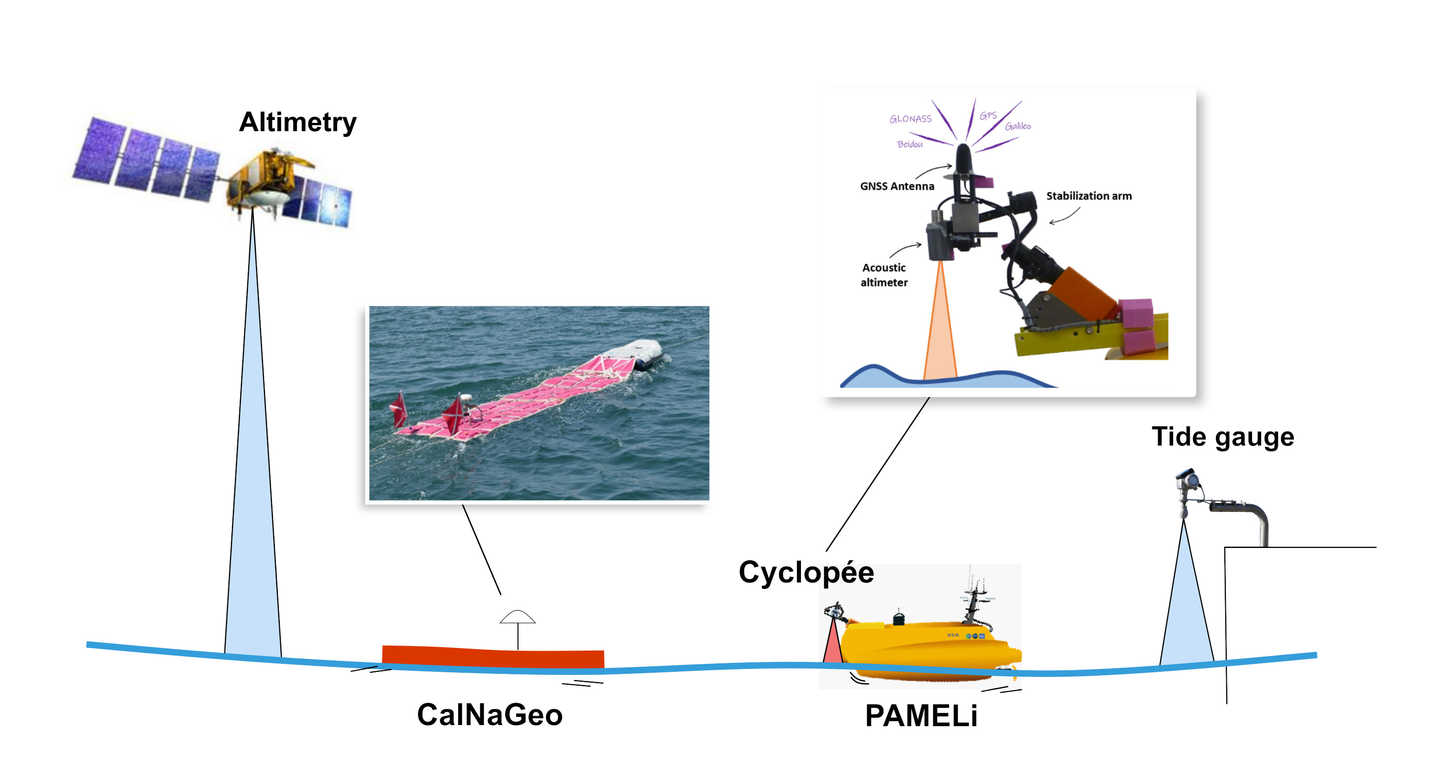
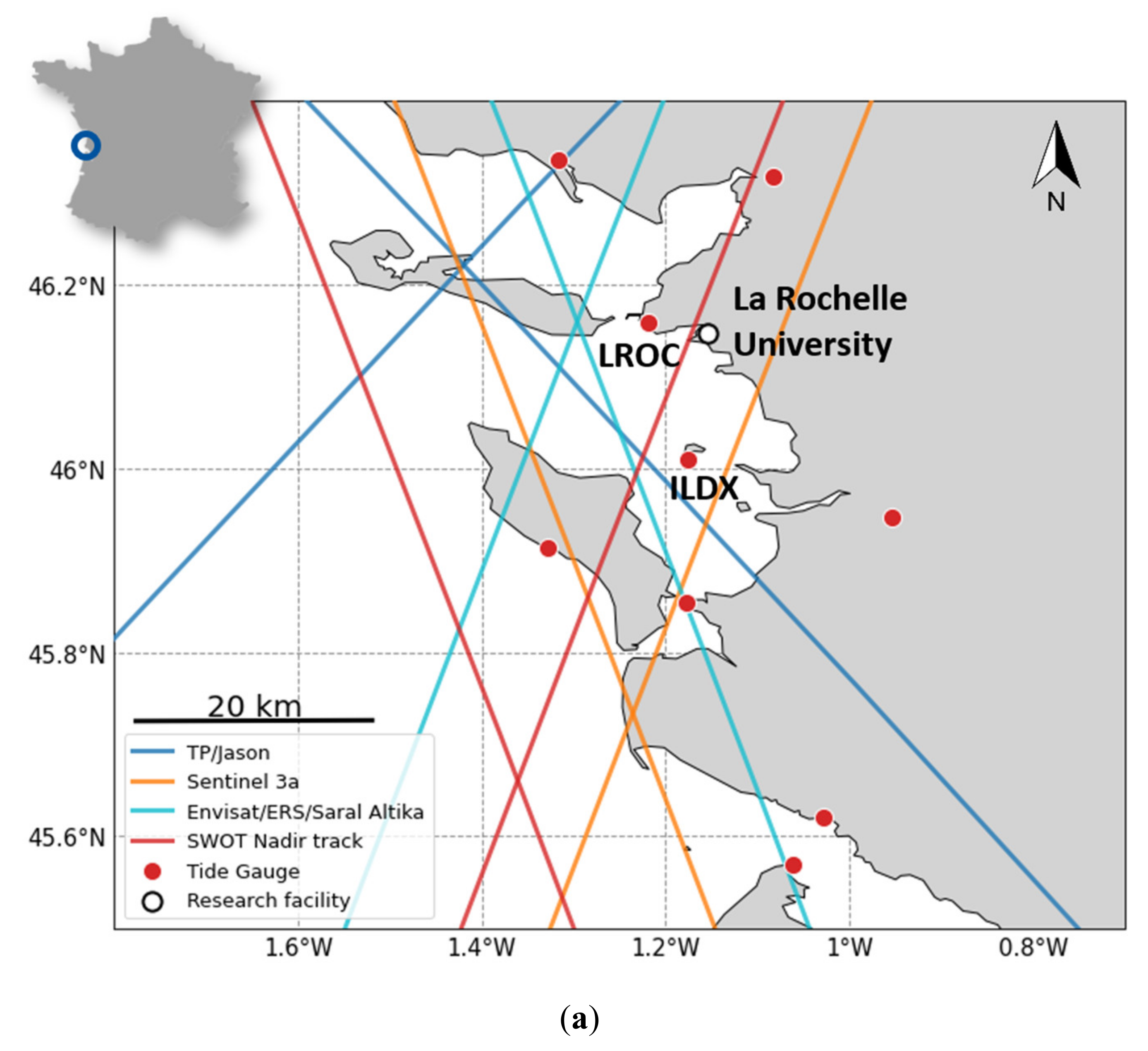
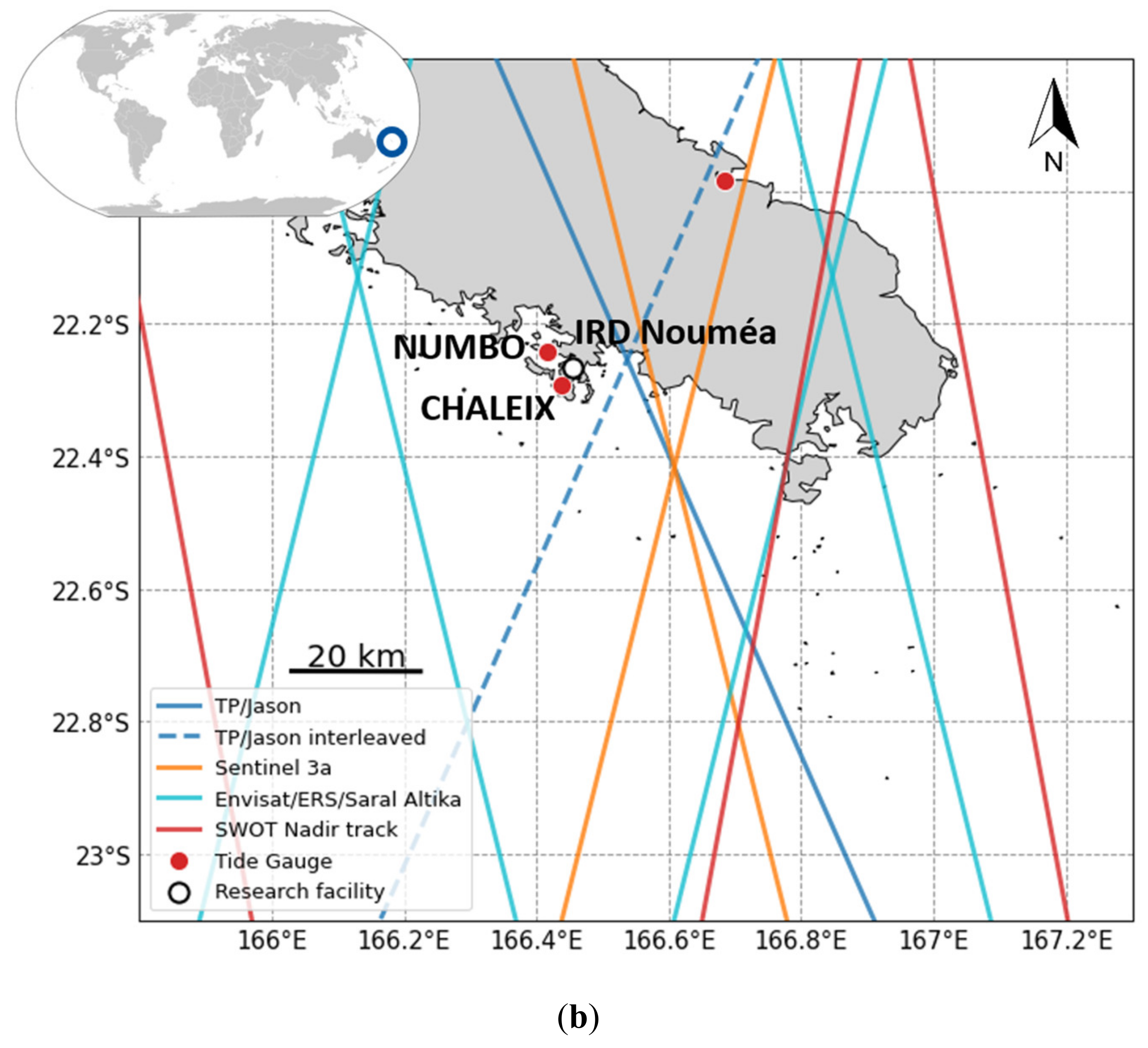
2.1. Coastal Areas for Calibration/Validation Activities

The tests presented in this paper were carried out in two specific coastal zones: The Pertuis Charentais area in France and the Noumea lagoon in New Caledonia.

On the west coast of France, the Pertuis Charentais is a rich coastal area which includes islands and estuaries (Figure 1a). The area is highly covered by nadir altimetry missions (Topex/Jason, SARAL, Sentinel-3) and the future SWOT mission. A large in-situ observation network has been developed, including a permanent observatory on Aix Island, which provides long time series of sea-level [17] using both tide gauge and vertical land motion information. At La Rochelle University, the LIENSs (Littoral Environnement et Sociétés) laboratory offers expertise and resources (boat, buoys, pressure sensors, etc.) to organize in-situ observation campaigns, including cal/val activities.

In New Caledonia, SSH mapping experiments were carried out in Noumea lagoon during a field campaign in October 2019. One of the objectives of the campaign was to improve SSH mapping methodology to model local geoid undulations under altimetric tracks. The area is covered by Topex/Jason (nominal and interleaved missions), Sentinel-3 and SWOT tracks (Figure 1b). The nearby CHALEIX and NUMBO tide gauges also provide a long sea-level record [18]. The proximity of the IRD (Institut de Recherche pour le Développement) research center in Noumea makes it possible to quickly set up field experiments and conduct studies to better understand the dynamics of the area.

These different configurations and dynamics of the two study areas allow us to tackle different scientific questions. Their land networks and nearby research infrastructures make them relevant for cal/val activities and to test new SSH mapping methodologies. They could also become good validation sites for the future SWOT mission.

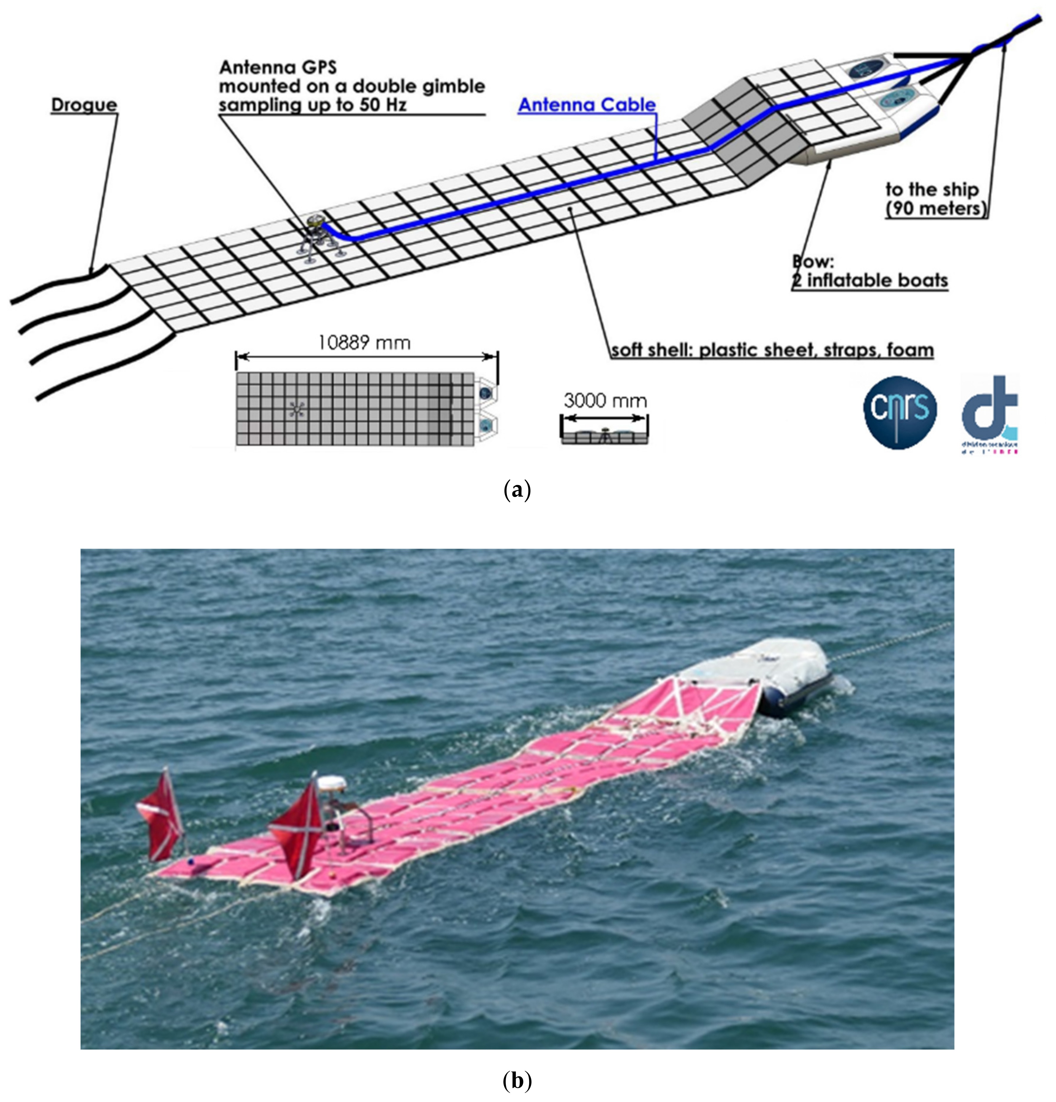
2.2. CalNaGeo GNSS Towed Carpet

The CalNaGeo GNSS floating carpet, developed by DT-INSU, can be towed for SSH mapping at high speed and in rough seas (the original design was for the Southern Ocean sea conditions). It is stable enough to keep its GNSS antenna quasi-horizontal to guarantee good signal quality and limit GNSS satellite track loss. The system consists of a geodetic GNSS antenna (Trimble Zephyr Rugged) mounted on a soft shell that follows the sea surface as seaweed follows swell and waves, ensuring a constant antenna height above sea surface. The antenna is mounted on a double gimble tied to the carpet and cabled to the receiver (Trimble NetR9), and batteries are located in one or two inflatable boats at the front of the system (the number of boats depends on the application, e.g., river/seashore versus open ocean) (Figure 2). The structure can be towed by a ship at up to 10 knots at several hundreds of meters to reduce the effect of boat’s wake.

The CalNaGeo system can be used for in-situ cal/val by SSH mapping, geoid measurement and wave monitoring, with recording rates up to 50 Hz. This design has been tested under various conditions: In the open ocean (Kerguelen, Noumea lagoon), in the coastal zone (Bangladesh, Pertuis Charentais and Corsica in France) and in rivers (Seine, Gironde in France).

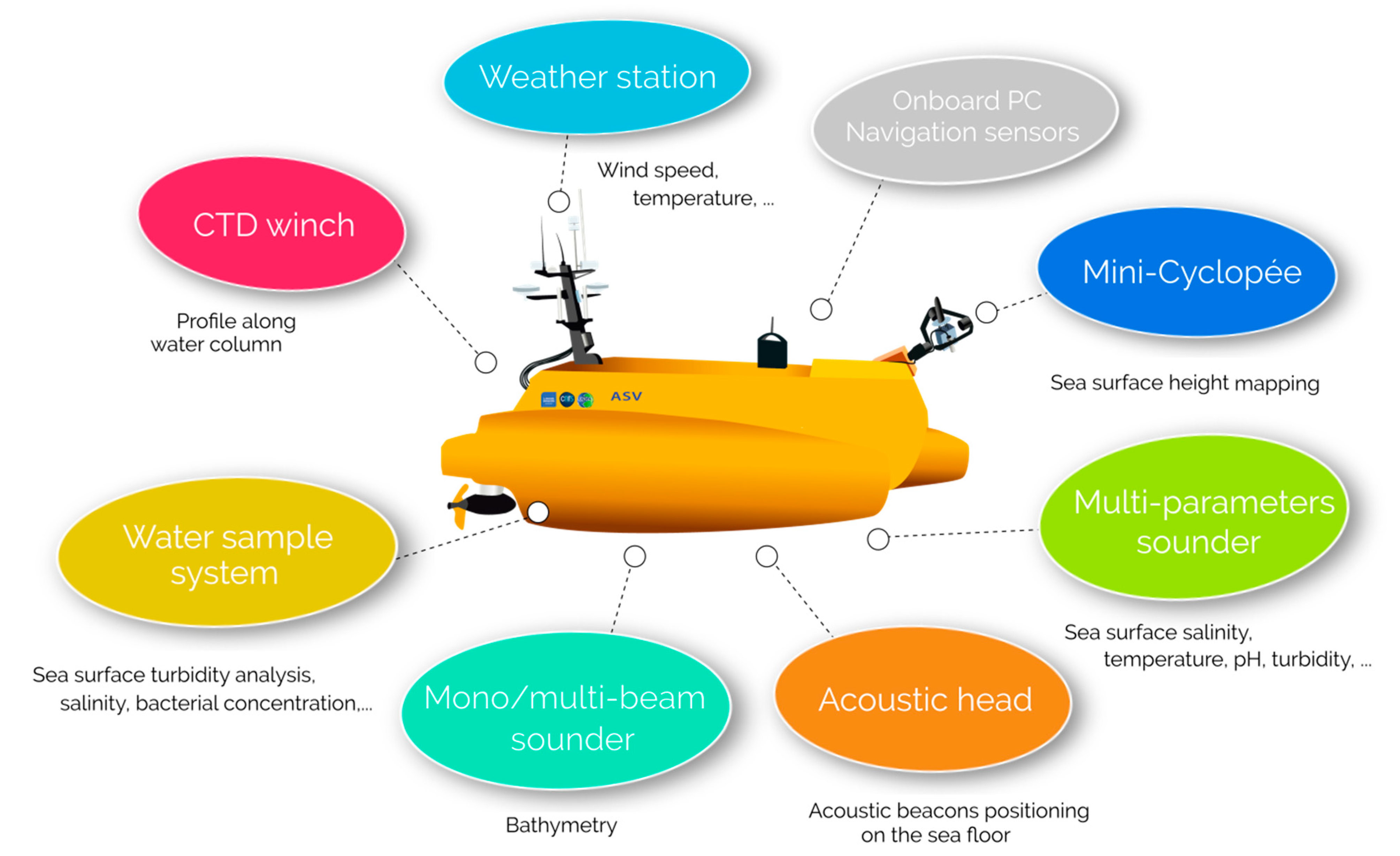
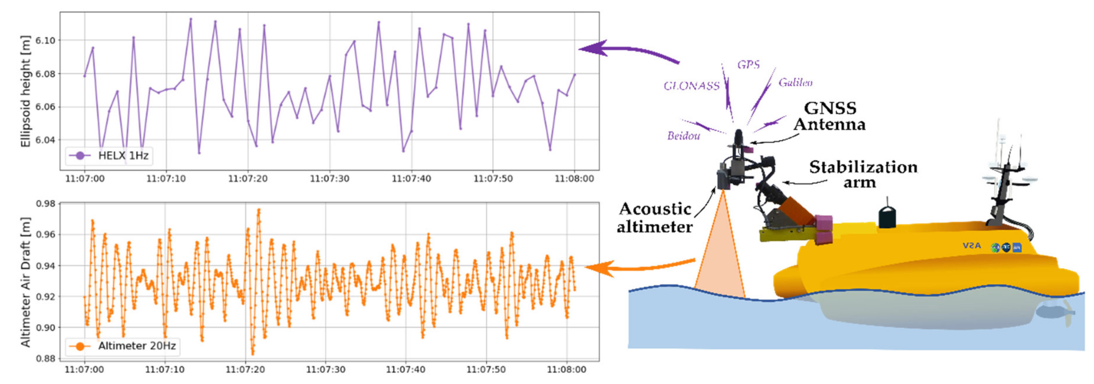
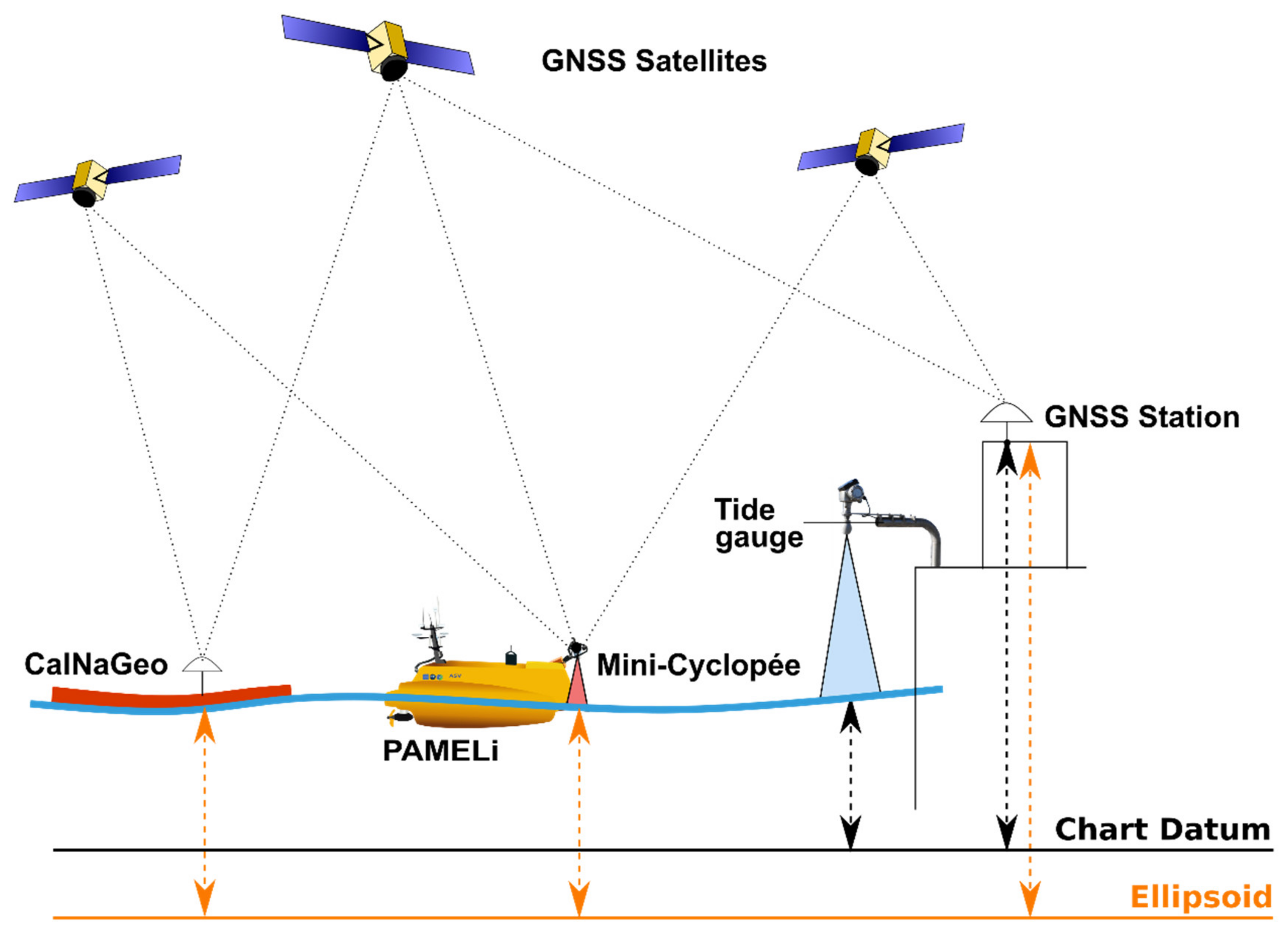
2.3. Cyclopée System with Autonomous Plateform

The second mapping system, developed by La Rochelle University and DT-INSU, is based on a USV named PAMELi (Plateforme Autonome Multicapteurs pour l’Exploration du Littoral—Project website: https://pameli.recherche.univ-lr.fr/). This project was born of the need for repeated, co-localized and simultaneous multidisciplinary observations to better monitor and understand the evolution of the coastal area. After each campaign, all collected data are saved to a shared database promoting interdisciplinary research development. This marine drone can support various sensors and can continuously monitor temperature, salinity, bathymetry and weather parameters during sea surface mapping [19] (Figure 3). This allows complete studies of the hydrodynamics in the coastal area, which will help cal/val of current and future altimeters.

The PAMELi USV is a C-CAT3 Catamaran built by L3Harris ASV. The design incorporates a large payload bay, and the two floats contain the batteries and small electric motors. At an average speed of 3–4 knots, PAMELi has an endurance of roughly 10 h, depending on sea conditions and payload. Unlike the CalNaGeo carpet, this platform provides its own propulsion and steering. Its modular construction makes it easy to deploy and combine scientific instruments above or below water, thanks to a lifting keel to support underwater instruments. The shallow draft (between 0.3 and 0.8 cm) and the small size of the vehicle (length: 3.02 m/width: 1.55 m) enables deployment in shallow areas. The vessel can be controlled manually or follow a pre-programmed route and integrates real-time camera viewing, useful in areas of significant maritime traffic. For safety reasons, due to heavy maritime traffic in the Pertuis Charentais, a ship follows PAMELi during one-day missions there. This support boat can tow the drone to the study area to save battery and also support the USV’s piloting system.

The PAMELi marine drone needs a dedicated sensor to monitor sea surface height. This is done using a continuous GNSS and air-draft sensor named Cyclopée, installed on the front of PAMELi (Figure 4). The philosophy of the Cyclopée system is to be a hybrid and compact SSH measuring tool that can be easily installed on various platforms (USV, small boats, catamaran). For small or low vessels, the name Mini-Cyclopée regroups all the designs with a small air-draft (~1 m), such as our experiments. For the mission in Les Pertuis Charentais, our Mini-Cyclopée system combines a GNSS Trimble BD940 receiver with a Harxon D-Helix Antenna for absolute positioning, and a SENIX Toughsonic 14 acoustic altimeter for air-draft measurements, both installed on a gyro-stabilization arm. A lighter version was also tested during the field campaign in Noumea lagoon: A GNSS Septentrio PolaRx5 receiver with Harxon D-Helix Antenna, and a Sonic Wave Sensor RV acoustic altimeter, mounted on a fixed arm.

Uncompensated acoustic altimeters have a well-known dependence on air temperature gradients [20]. For example, the French Hydrographic Service (Shom) detected errors up to 7 cm using the Brest-Penfeld acoustic altimeter for large air-draft [21]. Particular attention should be given to the choice of the acoustic sensor according to the estimated measurement range. In the case of the PAMELi USV, the air-draft is relatively low and constant, and therefore, an acoustic sensor was preferred to a radar altimeter because of its high-frequency measurement capacity (up to 20 Hz) without data loss. Both of the acoustic sensors we used are temperature compensated, and experiments are being developed to fully qualify the compensation accuracy.

3. Results

3.1. Instruments Calibration

In order to fully qualify these instruments, several field campaigns were performed. We first quantified these new instruments against well-qualified tide gauges in a so-called static mode (i.e., not moving horizontally), then we tested them in a kinematic mode to estimate the effect of speed on the water height measurements.

3.1.1. Static Tide Gauge Sessions

Setup of the Experiments 

During these experiments, all instruments are placed near a tide gauge, either moored to a pier or the seafloor, or dynamically holding station on the water. This installation depends on the system, the weather conditions and experiment duration. These static sessions are organized during neap tide period (e.g., the period of moderate tide) with calm weather conditions to be able to keep systems stationary. The observed sea-level variations and resulting heights are then compared to the reference tide gauge (Figure 5).

For the computation, differential GNSS observations are processed at 1Hz using the RTKLib software [22] and permanent GNSS stations of the French permanent GNSS network (RGP-IGN—http://rgp.ign.fr/) and New Caledonia Direction des Infrastructures, de la Topographie et des Transports Terrestres (DITTT—https://dittt.gouv.nc). In all cases, the baseline length between the instrument and the reference GNSS station is less than 150 m, allowing us to discard tropospheric and ionospheric corrections, as well as orbital and clock errors (RTKLib processing options are detailed in Supplementary Material—Table S1).

After a first data selection to keep only positions with more than four satellites and remove outliers deviating more than 4σ from the average, GNSS heights are filtered using the Vondrak filter [23], which allows us to process data series with gaps and reduces the amplitude of artificial short period signals (spectrum overlapping). A cut-off period of 120 s was chosen to filter out short-wavelength oscillations [14]. All GNSS sea-level heights initially referenced to the IAG GRS 80 ellipsoid were reduced to chart datum using precise leveling information from the French Hydrographic Service (Shom—https://www.shom.fr/) and our own measurements. Since our experiments are co-located with well-characterized tide gauges which are linked to the WGS84 geodetic system, we can tie all our measurements to chart datum (Figure 5). To be consistent with 1Hz GNSS observations, 1 Hz tide gauge data provided by the Shom are used for both static sessions. As GNSS times-series, tide gauge observations are filtered with a Vondrak filter with a 120 s cutoff period. Results of two static sessions are presented here.

The first static session was conducted on 27 June 2019 during the first field experiment with PAMELi in the Pertuis Charentais area in France. For 27 min, the CalNaGeo coastal carpet and PAMELi USV Mini-Cyclopée systems measured SSH at 150 m and 20 m, respectively, from the Aix Island tide gauge (ILDX tide gauge, Figure 1a). A 2-min gap in tide gauge data reduced the comparison time span to 25 min (Figure 6a).

The second static session was conducted on 8 October 2019 in Noumea Lagoon. For seven hours, the CalNaGeo coastal carpet, a version of Mini-Cyclopée mounted on the wharf, and a GNSS Buoy (Figure 7a) measured SSH next to Numbo tide gauge (NUMBO tide gauge, Figure 1b). The GNSS buoy was already used in field campaigns and demonstrates its capability to provide sea-level records with sub-centimetric uncertainty [8,24]. We also used leveling operations to compare the Mini-Cyclopée altimeter-only SSH with GNSS + altimeter SSH.

Comparison with Tide Gauge Observations 

To assess the performance of the GNSS instruments, the radar tide gauge is taken as the reference instrument for each static session. We created Van de Casteele diagrams (Figure 6c and Figure 7c), commonly used to control tide gauge performance versus a reference probe [25], by plotting the reference tide gauge water level minus the sensor observations (x-axis) versus the tide gauge water level (y-axis). If the instrument is not biased and/or delayed compared to the tide gauge, the result of the Van de Casteele diagram shows a vertical line centered at zero.

For the Les Pertuis session (Figure 6c), Van de Casteele diagrams for the GNSS carpet (red) and PAMELi Mini-Cyclopée (violet) are vertical, but show a bias of 2.1 cm ± 0.3 and 2.0 cm ± 0.3 respectively. Despite this bias, which could result from a referencing error or a height inaccuracy, due to the GNSS processing method, the two sensors are very consistent. To be truly complete, this test should be performed over a full tide cycle.

For the Noumea session (Figure 7c), Van de Casteele diagrams for the GNSS carpet (red) and GNSS buoy (blue) show a bias of 0.6 cm ± 0.4 and −1.7 cm ± 0.5 respectively. Uncertainties remain regarding the distance from the GNSS Antenna Reference Point (ARP) to sea-level. Aside from this vertical bias, the GNSS carpet and GNSS buoy observations are consistent with the Numbo radar tide gauge.

The Van de Casteele diagram of the acoustic altimeter only (Figure 7c, orange) shows a linear slope indicating a scale error. This error is being investigated and may be due to air temperature variations. As noted in Section 2.3, acoustic sensors could have a dependence on air temperature gradient up to several cm if not compensated by internal measurements. The variation of the altimeter beam footprint size with air-draft could also play a role, and tests are underway to estimate this effect. However, over the entire Noumea lagoon session, the mean air-draft measured by the acoustic sensor is around 1.25 m. At this draft, the sensor bias is less than 1 cm (Supplementary Material—Figure S1), which is in the range of the GNSS measurement uncertainties. When combining this air-draft with the HELIX GNSS position (Figure 7c, violet), the Van de Casteele diagram trend is less clear. At this location, GNSS measurements are noisier than usual, probably due to local multipathing and masking (metal guardrail).

These sessions indicate that, for all instruments, residuals between SSH measurements and a radar tide gauge (i.e., including the bias of the instrument) are below 2.1 cm (

Table 1. Statistics of the residuals obtained against radar tide gauge used as a reference during static sessions. For the Pertuis session (resp. Noumea), the referenced tide gauge is ILDX (Aix Island, resp. NUMBO).

System			Pertuis Session			Noumea Session
			Mean Difference to TG [m]	Std [m]	Number of Data	Mean Difference to TG [m]	Std [m]	Number of Data
CalNaGeo			0.021	0.003	1 487	0.006	0.004	24 543
Mini-Cyclopée	On USV		0.020	0.003	1 492	-	-	-
	On wharf	Altimeter only	-	-	-	0.014	0.005	25 380
		Altimeter and GNSS	-	-	-	0.002	0.009	22 814
GNSS Buoy			-	-	-	−0.017	0.005	22 705

). As for their accuracy, an absolute bias of 1–2 cm with respect to the tide gauge was observed on these short sessions. Uncertainties remain regarding terrestrial geodesy measurements and GNSS processes which could have a significant impact on the vertical component at the cm-level. In addition to the biases induced by the GNSS calculation, it is also important to use instruments with well-known technical characteristics, such as GNSS antennas with absolute or at least relative calibration. Nevertheless, for longer averaged time-series, this absolute bias could be reduced to a mm-level as in the Corsica calibration site [26], because some errors in the GNSS processing (orbit, clock, ionospheric and tropospheric corrections) cannot be correctly averaged over sessions of few hours of measurements.

Despite the absolute bias, the systems are stable and precise even over short measurement periods, with a standard deviation on the filtered time series residuals of around 4 mm. This indicates that these new systems are now comparable in terms of precision with the best available tide gauge systems, even if the systematic errors need to be further investigated.

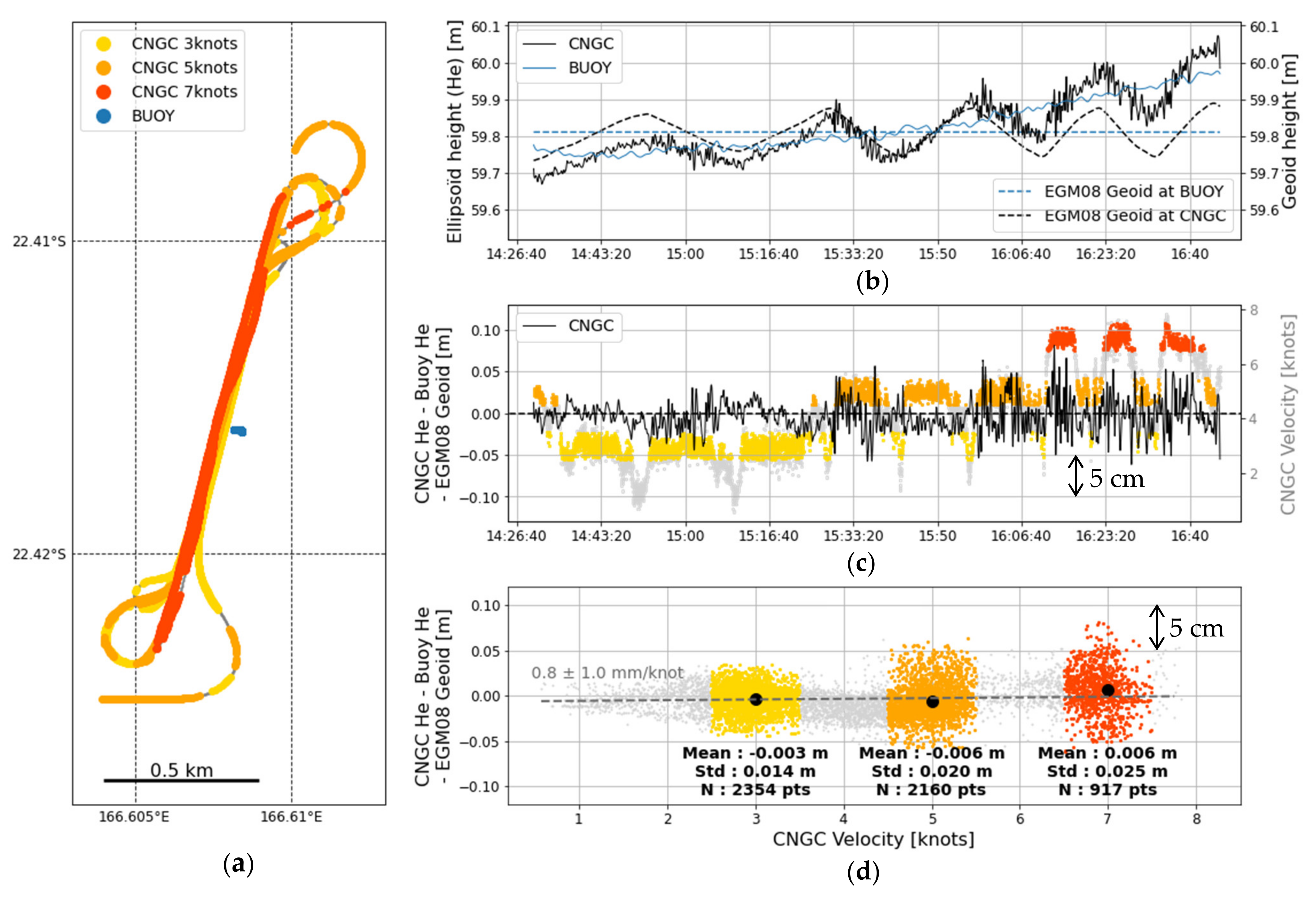
3.1.2. Effect of Speed on Water Height Measurements

CalNaGeo Experiment Setup in Noumea Lagoon 

One of the main challenges with kinematic GNSS sea-level mapping systems is to continuously monitor the GNSS antenna height above the water level (air-draft), which can vary with the load and speed of the platform. As the velocity increases, a boat’s hull lifts out water (hereafter named “planing effect”), potentially inducing biases in the GNSS vertical component.

To quantify the effect of CalNaGeo GNSS carpet velocity variations on planing effects, a dedicated experiment was conducted in calm weather in Noumea Lagoon on 15 October 2019. The coastal version of the GNSS carpet was towed by R/V ALIS successively at 3, 5, and 7 knots along a 950 m SSW-NNE profile. The profile was repeated three times for each velocity, for a total of nine profiles (Figure 8a). During the 2 h experiment duration, a GNSS buoy moored in the middle of the profile measured sea-level height variations. The distance between the GNSS carpet and the GNSS buoy varies between 45 m and 400 m.

As the experiment took place more than 40km from the nearest permanent GNSS station, the GNSS processing was carried out with the GINS software in Precise Point Positioning (PPP) mode [27]. The kinematic PPP mode computes a single GNSS receiver’s position without the need for a reference station. This method has already been shown capable of computing GNSS buoy height within a few centimeters [10]. GINS processing options used to compute GNSS carpet and GNSS buoy positions during this experiment are detailed in Supplementary Material—Table S2.

GNSS carpet and buoy time series are edited to keep positions with more than 4 satellites and remove points deviating more than 4σ from the average. Time series are then filtered with a Vondrak filter with a 120 s cutoff period. The EGM08 geoid model [5] is used to subtract long-wavelength signals from the carpet and buoy observations (Figure 8b). We used a 0.005° × 0.005° local EGM08 geoid grid computed online thanks to International Centre for Global Earth Model (ICGEM) services (http://icgem.gfz-potsdam.de/) and linearly interpolated along CalNaGeo track and at buoy position with Python tools. Along the profile, the geoid gradient is about 7cm/km. We use the sea surface height measurements of the GNSS buoy to remove the non-velocity related variations from the CalNaGeo carpet data (tide, atmospheric effects, etc.). The difference between GNSS carpet and buoy heights represents dynamic variations measured by the carpet along profiles (Figure 8c, black line).

Observations are noisier as the velocity increases, with SSH standard deviation increasing from σ = 1.4 cm at 3 knots to σ = 2.5 cm at 7 knots (Figure 8d). However, the average difference in SSH observed by the GNSS carpet and the GNSS buoy remains sub-centimetric along straight profiles, as well as during turns. We observe a waterline variation of about 0.8 ± 1 mm/knot, largely dominated by noise at high speed, which agrees with previous speed tests in Corsica (Supplementary Materials—Figure S3). According to these results, the towing speed of CalNaGeo does not affect its height measurements. The observed differences are not characteristic of a planning effect and may instead be a consequence of GNSS height computations.

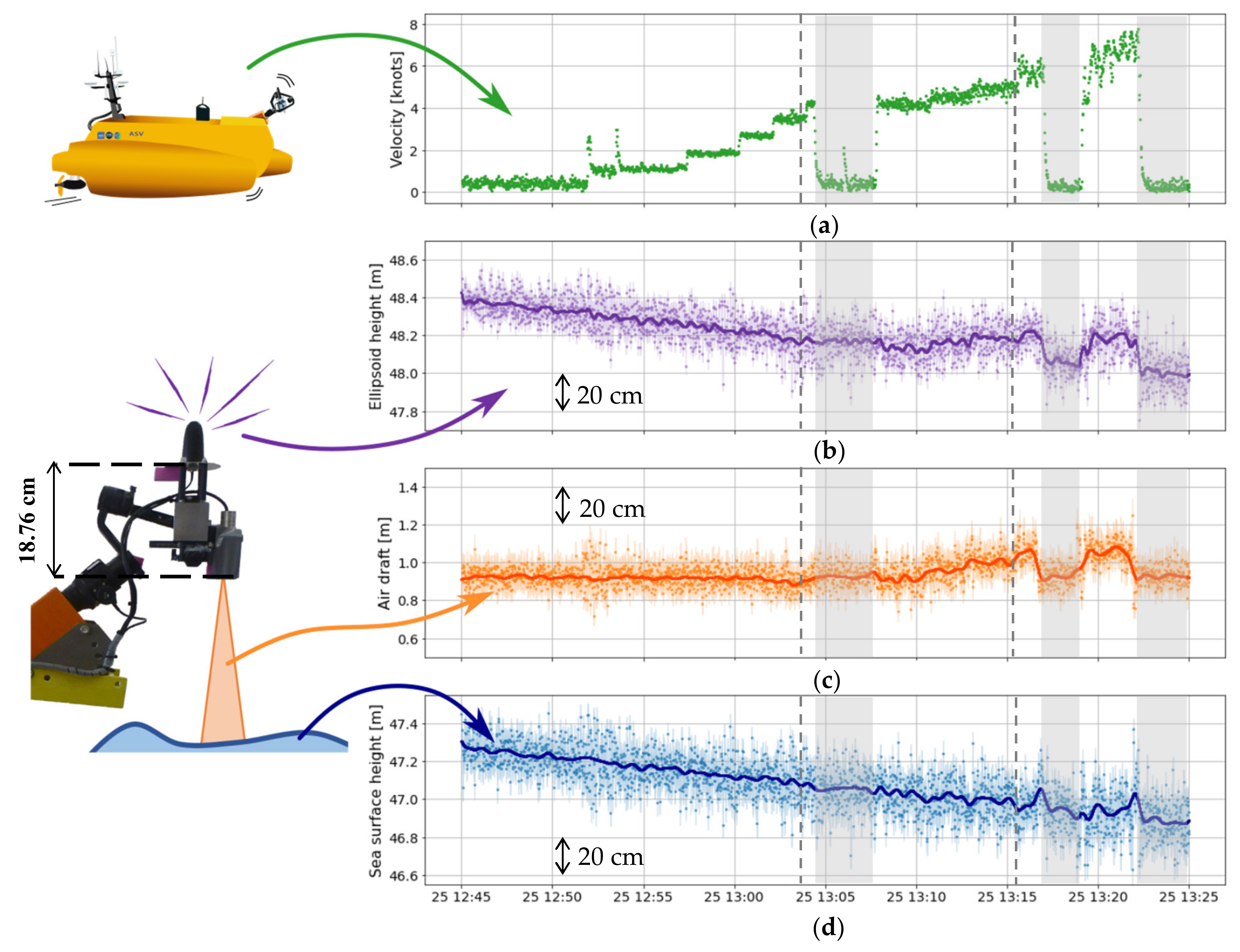
PAMELi Experiment Setup Near La Rochelle 

On 25 June 2019, several offshore tests were carried out near La Rochelle to characterize PAMELi USV maneuverability. We design a speed test to quantify the effect of the velocity variations on Mini-Cyclopée water height measurements. PAMELi USV was driven in calm seas at different speeds from 3 to 7 knots (Figure 9a) along a 2.9 km profile for 45 min.

We use the GINS PPP solution to compute the position of Mini-Cyclopée HELIX antenna (Figure 9b). GNSS processing is detailed in Supplementary Material—Table S2. The GNSS time series is edited to keep positions with more than four satellites and remove points deviating more than 4σ from the average. We then subtract from the GNSS heights: The GNSS time-interpolated air-draft values of the acoustic altimeter (Figure 9c) plus the 18.76 cm offset between GNSS antenna and acoustic altimeter base reference point. The result is the Mini-Cyclopée SSH time series (Figure 9d).

We observe that, up to 4 knots, the vessel is stable, and speed does not affect GNSS measurements significantly. Above 4 knots, GNSS and acoustic altimeter observations are noisier, but the acoustic air-draft measurements allow us to correct GNSS heights and obtain proper sea-level measurement up to a speed of 7 knots or if the drone stops. Thanks to the combination of GNSS and the acoustic altimeter, it is possible to map sea surface variations in motion using the PAMELi system at up to 7 knots without significant effect on the mean SSH.

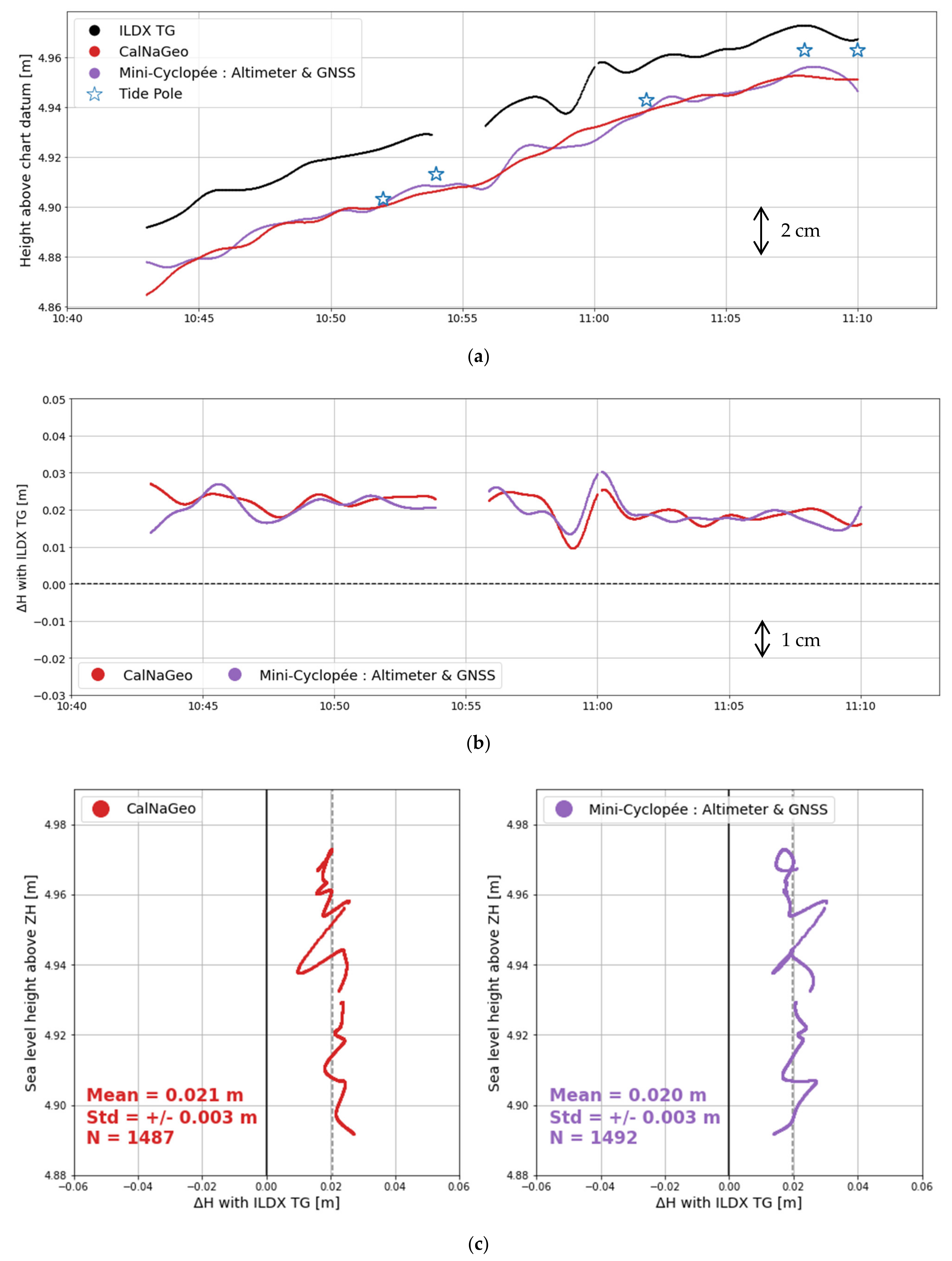
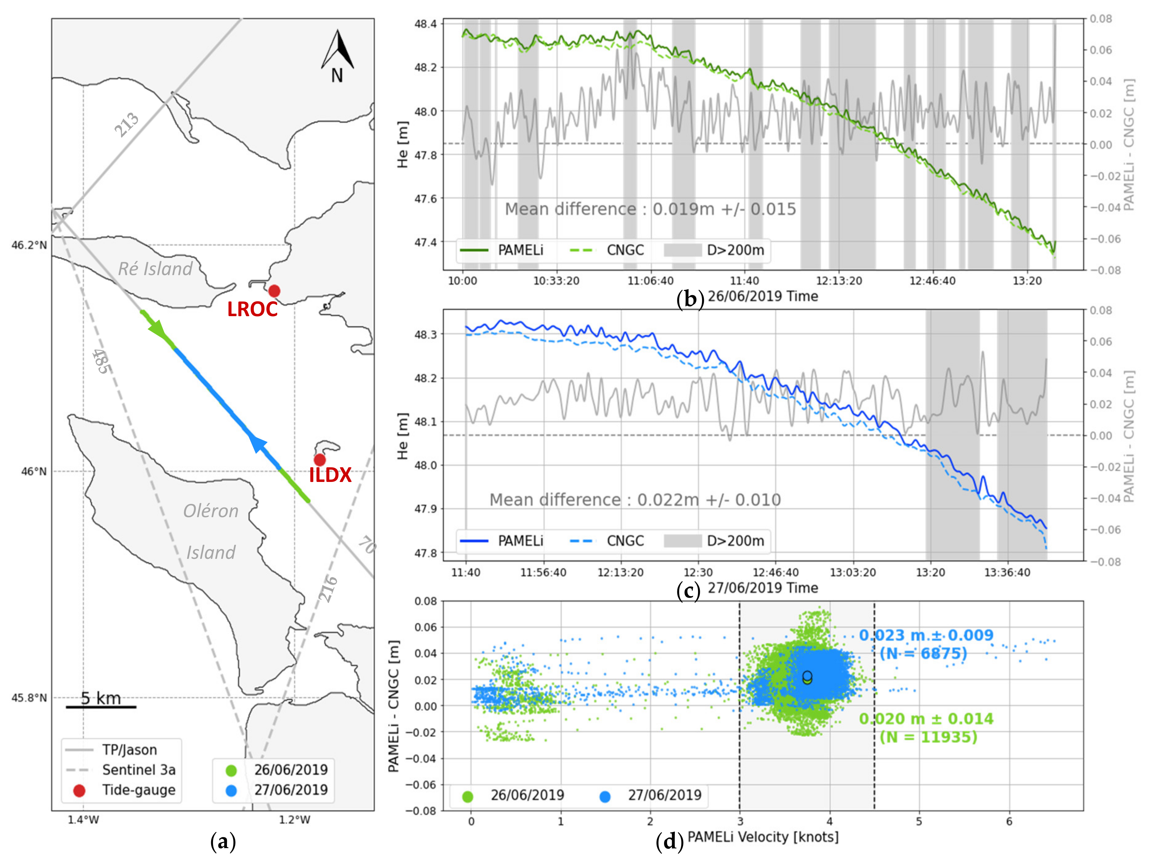
3.2. Comparison of Both Systems

The prior section aimed to separately quantify the CalNaGeo and Mini-Cyclopée systems. In this section, we compare their kinematic SSH measurements along the same profile and under the same weather conditions.

Sea Surface Measurements along Track 

The June 2019 experiment in Les Pertuis Charentais area was designed to compare CalNaGeo towed carpet sea surface measurements with Mini-Cyclopée mounted on PAMELi. On two consecutive days (26 and 27 June 2019), the two systems mapped SSH under trace 70 of the Jason 3 altimetric mission. During these two days, CalNaGeo and PAMELi USV covered the 15 km track at an average speed of 3.5 knot and with a mean spacing of 190 m (Figure 10a). The mission was carried out during a neap tide period with calm weather and sea conditions.

As the distance with the Aix Island permanent GNSS stations is less than 20 km, we use the RTKLib differential method to compute the GNSS solutions (processing parameters are detailed in Supplementary Material—Table S1). After a data selection to keep positions with more than four satellites and without outliers, CalNaGeo data are filtered with a 120 s Vondrak filter. The same method was used for the Mini-Cyclopée positions, but the 120 s Vondrak filtered is applied after a combination of the HELIX ellipsoid heights with the 1 Hz acoustic altimeter air-draft. A cutoff period of 120 s for the Vondrak filter keep signals longer than 200 m at a mean speed of 3.5 knot. The resulting ellipsoid heights for the two sessions are shown in Figure 10b,c. The slope observed in the resulting heights is mainly due to tidal variations.

The mean difference between Mini-Cyclopée and CalNaGeo SSH measurement are 1.9 +/− 1.5 cm and 2.2 +/− 1.0 for the first and second sessions, respectively. Neither the distance between the two instruments nor the velocity significantly impacts those differences (Figure 10). This shows that, beyond systematics errors induced by GNSS processing or geodesic measurements, the two kinematic GNSS methods are consistent to measure SSH in motion at a centimetric level.

4. Discussion

In static mode, CalNaGeo shows a bias of, respectively, 2.1 cm ± 0.3 and 0.6 cm ± 0.4 with the ILDX and NUMBO tide gauges, demonstrating the good performance of this design to measure sea-level heights variations. It is noticeable that this system has comparable performance in static mode than the classical GNSS buoy system widely used for satellite altimetry calibration [8]. In kinematic mode, the GNSS carpet has no height bias dependency with velocity, confirming previous preliminary experiments [28]. Moreover, this system has demonstrated its robustness when towed in harsh condition in the Southern Ocean in 2016 with 60 knots wind and 4m waves. CalNaGeo towed carpet can be used in the shallow coastal area, as well as in the open ocean—but the GNSS carpet is not easily transportable because of its large dimensions, and the towing-constraint makes it difficult to maneuver in areas with heavy marine traffic.

The Mini-Cyclopée system also provides SSH consistent with tide gauges with an absolute bias of, respectively, 2.0 cm ± 0.3 and 0.2 cm ± 0.9 with the ILDX and NUMBO tide gauges. Thanks to the combination of a GNSS antenna and an acoustic altimeter, this system can provide reliable SSH measurements up to a speed of 7 knots. However, the use of an acoustic altimeter and its dependence on air temperature variations may impact the final accuracy. Particular attention should be given to the choice of the acoustic sensor depending on the estimated measurement range and field constraints, and a complete qualification of the sensors is necessary to ensure proper measurements.

Uncertainties remain about the accuracy of these GNSS systems, both in terms of system biases and GNSS processing. Technically, it is also important to determine all instrumental offsets and to use instruments with well-known technical characteristics, such as GNSS antenna calibrations. For example, the HARXON D-Helix antenna used in this paper lacks an antenna phase map. The choice of processing methods (differential mode, PPP (float or integer), etc.) could also have a significant impact on cm-level vertical measurements. Experimental conditions (local sea and weather conditions, GNSS satellites coverage, etc.) may also limit positioning accuracy. Improvements are possible using, for example, multi-constellation GNSS, orbit/clocks product developments, integer ambiguity resolution.

Compared to the GNSS carpet, the Mini-Cyclopée mounted on a USV or a boat is compact and maneuverable, especially in shallow coastal areas with dense marine traffic. For offshore campaigns, other systems like the “GNSS Wave-glider” [16] have proven their capacity to map SSH with a centimetric level and complete energy autonomy. Installed on a multi-sensor platform like PAMELi, Mini-Cyclopée can also combine sea surface height measurements with several environmental parameters like sea surface salinity or sea surface temperature (SST), bathymetry, atmospheric parameters, etc. This can allow integrated studies of coastal waters dynamic that could be essential for in-situ calibration of current and future satellite altimeter missions, such as the SWOT mission.

5. Conclusions

In this article, we presented a selection of tests to illustrate the ability of the CalNaGeo GNSS carpet and the Cyclopée systems to precisely measure SSH in motion. Both have advantages and disadvantages that need to be considered to match user expectations and field constraints. Static comparisons with radar tide gauges show that, despite an absolute bias, these systems are stable and precise with a standard deviation of a few millimeters on the residuals. In motion, velocity does not significantly affect SSH measurements, and a kinematic along profile comparison demonstrates that the two systems provide maps of SSH variations that are consistent on a centimetric level.

The Pertuis Charentais area and Noumea Lagoon used in this study are well-suited for future cal/val activities. Both sites are highly covered by past and current nadir altimetry missions and the future SWOT mission, and bring together large communities interested in scientific quantification of sea-level variations and their societal and environmental impacts.

References

1. Bonnefond, P.; Exertier, P.; Laurain, O.; Thibaut, P.; Mercier, F. GPS-based sea level measurements to help the characterization of land contamination in coastal areas. Adv. Space Res. 2013, 51, 1383–1399. [Google Scholar] [CrossRef]
2. Roblou, L.; Lamouroux, J.; Bouffard, J.; Lyard, F.; Le Hénaff, M.; Lombard, A.; Marsaleix, P.; De Mey, P.; Birol, F. Post-processing Altimeter Data Towards Coastal Applications and Integration into Coastal Models. In Coastal Altimetry; Vignudelli, S., Kostianoy, A.G., Cipollini, P., Benveniste, J., Eds.; Springer: Berlin/Heidelberg, Germany, 2011; pp. 217–246. ISBN 978-3-642-12796-0. [Google Scholar]
3. GCOS. Systematic Observation Requirements for Satellite-Based Products for Climate 2011 Update: Supplemental Details to the Satellite-Based Component of the “Implementation Plan for the Global Observing System for Climate in Support of the UNFCCC (2010 Update); WMO: Geneva, Switzerland, 2011. [Google Scholar]
4. Mitchum, G.T. An Improved Calibration of Satellite Altimetric Heights Using Tide Gauge Sea Levels with Adjustment for Land Motion. Mar. Geod. 2000, 23, 145–166. [Google Scholar] [CrossRef]
5. Pavlis, N.K.; Holmes, S.A.; Kenyon, S.C.; Factor, J.K. The development and evaluation of the Earth Gravitational Model 2008 (EGM2008). J. Geophys. Res. 2012, 117. [Google Scholar] [CrossRef] [Green Version]
6. Ray, R.D.; Egbert, G.D.; Erofeeva, S.Y. Tide Predictions in Shelf and Coastal Waters: Status and Prospects. In Coastal Altimetry; Vignudelli, S., Kostianoy, A.G., Cipollini, P., Benveniste, J., Eds.; Springer: Berlin/Heidelberg, Germany, 2011; pp. 191–216. ISBN 978-3-642-12796-0. [Google Scholar]
7. Born, G.H.; Parke, M.E.; Axelrad, P.; Gold, K.L.; Johnson, J.; Key, K.W.; Kubitschek, D.G.; Christensen, E.J. Calibration of the TOPEX altimeter using a GPS buoy. J. Geophys. Res. 1994, 99, 24517. [Google Scholar] [CrossRef]
8. André, G.; Miguez, B.M.; Ballu, V.; Testut, L.; Wöppelmann, G. Measuring sea level with gps-equipped buoys: A multi-instruments experiment at Aix Island. Int. Hydrogr. Rev. 2013, 14, 26–38. [Google Scholar]
9. Bonnefond, P.; Haines, B.J.; Watson, C. In situ Absolute Calibration and Validation: A Link from Coastal to Open-Ocean Altimetry. In Coastal Altimetry; Vignudelli, S., Kostianoy, A.G., Cipollini, P., Benveniste, J., Eds.; Springer: Berlin/Heidelberg, Germany, 2011; pp. 259–296. ISBN 978-3-642-12796-0. [Google Scholar]
10. Fund, F.; Perosanz, F.; Testut, L.; Loyer, S. An Integer Precise Point Positioning technique for sea surface observations using a GPS buoy. Adv. Space Res. 2013, 51, 1311–1322. [Google Scholar] [CrossRef]
11. Rocken, C.; Johnson, J.; Van Hove, T.; Iwabuchi, T. Atmospheric water vapor and geoid measurements in the open ocean with GPS. Geophys. Res. Lett. 2005, 32. [Google Scholar] [CrossRef] [Green Version]
12. Bouin, M.-N.; Ballu, V.; Calmant, S.; Boré, J.-M.; Folcher, E.; Ammann, J. A kinematic GPS methodology for sea surface mapping, Vanuatu. J. Geod. 2009, 83, 1203–1217. [Google Scholar] [CrossRef]
13. Foster, J.H.; Carter, G.S.; Merrifield, M.A. Ship-based measurements of sea surface topography. Geophys. Res. Lett. 2009, 36, L11605. [Google Scholar] [CrossRef]
14. Bonnefond, P.; Exertier, P.; Laurain, O.; Ménard, Y.; Orsoni, A.; Jeansou, E.; Haines, B.J.; Kubitschek, D.G.; Born, G. Leveling the Sea Surface Using a GPS-Catamaran. Mar. Geod. 2003, 26, 319–334. [Google Scholar] [CrossRef]
15. Crétaux, J.-F.; Bergé-Nguyen, M.; Calmant, S.; Romanovski, V.V.; Meyssignac, B.; Perosanz, F.; Tashbaeva, S.; Arsen, A.; Fund, F.; Martignago, N.; et al. Calibration of Envisat radar altimeter over Lake Issykkul. Adv. Space Res. 2013, 51, 1523–1541. [Google Scholar] [CrossRef]
16. Penna, N.T.; Maqueda, M.A.M.; Martin, I.; Guo, J.; Foden, P.R. Sea Surface Height Measurement Using a GNSS Wave Glider. Geophys. Res. Lett. 2018, 45, 5609–5616. [Google Scholar] [CrossRef]
17. Gouriou, T.; Martín Míguez, B.; Wöppelmann, G. Reconstruction of a two-century long sea level record for the Pertuis d’Antioche (France). Cont. Shelf Res. 2013, 61–62, 31–40. [Google Scholar] [CrossRef]
18. Aucan, J.; Merrifield, M.A.; Pouvreau, N. Historical Sea Level in the South Pacific from Rescued Archives, Geodetic Measurements, and Satellite Altimetry. Pure Appl. Geophys. 2017, 174, 3813–3823. [Google Scholar] [CrossRef]
19. Coulombier, T.; Ballu, V.; Pineau, P.; Lachaussee, N.; Poirier, E.; Guillot, A.; Calzas, M.; Drezen, C.; Fichen, L.; Plumejeaud, C.; et al. PAMELi, un drone marin de surface au service de l’interdisciplinarité. In Proceedings of the XVèmes Journées Nationales Génie Côtier–Génie Civil, La Rochelle, France, 29–31 May 2018; pp. 337–344. [Google Scholar]
20. Martín Míguez, B.; Le Roy, R.; Wöppelmann, G. The Use of Radar Tide Gauges to Measure Variations in Sea Level along the French Coast. J. Coast. Res. 2008, 4, 61–68. [Google Scholar] [CrossRef] [Green Version]
21. Roy, R.L. Evaluation of the Quality of Radar Telemeters. Available online: https://www.sonel.org (accessed on 25 June 2020).
22. Takasu, T. RTKLIB: An Open Source Program Package for GNSS Positioning. Available online: http://www.rtklib.com/ (accessed on 6 June 2020).
23. Vondrak, J. Problem of Smoothing Observational Data II; Astronomicall Institue of the Czechoslovak Academy of Sciences: Praha, Czech, 1977; Volume 28, pp. 84–89. [Google Scholar]
24. Gobron, K.; de Viron, O.; Wöppelmann, G.; Poirier, É.; Ballu, V.; Van Camp, M. Assessment of Tide Gauge Biases and Precision by the Combination of Multiple Collocated Time Series. J. Atmos. Ocean. Technol. 2019, 36, 1983–1996. [Google Scholar] [CrossRef] [Green Version]
25. Miguez, B.M.; Testut, L.; Wöppelmann, G. The Van de Casteele Test Revisited: An Efficient Approach to Tide Gauge Error Characterization. J. Atmos. Oceanic Technol. 2008, 25, 1238–1244. [Google Scholar] [CrossRef]
26. Bonnefond, P.; Exertier, P.; Laurain, O.; Guinle, T.; Féménias, P. Corsica: A 20-Yr multi-mission absolute altimeter calibration site. Adv. Space Res. 2019. [Google Scholar] [CrossRef]
27. Marty, J.C.; Loyer, S.; Perosanz, F.; Mercier, F.; Bracher, G.; Legresy, B.; Portier, L.; Capdeville, H.; Fund, F.; Lemoine, J.M.; et al. GINS: The CNES/GRGS GNSS scientific software. In Proceedings of the ESA Proceedings WPP326, Copenhagen, Denmark, 31 August–2 September 2011. [Google Scholar]
28. Calzas, M.; Brachet, C.; Drezen, C.; Fichen, L.; Guillot, A.; Téchiné, P.; Testut, L.; Bonnefond, P.; Laurain, O.; Umr, G.; et al. Mesure du geoïde marin avec le système CalNaGEO (GNSS). 2019. Available online: http://www.legos.obs-mip.fr/observations/rosame/documents/CalNaGEO_Refmar_2019.pdf?lang=fr (accessed on 12 August 2020).
Figure 1. Study areas and altimetry coverage; (a) The Pertuis Charentais area near La Rochelle, in the west coast of France; (b) Noumea lagoon in New Caledonia.
Remotesensing 12 02656 g001aRemotesensing 12 02656 g001b
Figure 2. (a) A general drawing of the original CalNaGeo offshore towed carpet with a double inflatable boat in front (© M.Calzas—DT-INSU); (b) CalNaGeo coastal carpet in the Pertuis Charentais area.
Remotesensing 12 02656 g002
Figure 3. PAMELi (Plateforme Autonome Multicapteur pour l’Exploration du Littoral), a multi-sensor platform for coastal observations (© T. Guyot—LIENSs).
Remotesensing 12 02656 g003
Figure 4. Mini-Cyclopée measuring system used on PAMELi unmanned surface vehicle (USV): To continuously monitor the sea surface height, this sensor combines a geodetic Global Navigation Satellite Systems (GNSS) antenna with an acoustic altimeter which allows for air-draft corrections. Note that for all our datasets, altimeter measures at 20 Hz, while GNSS is programmed to make 1 Hz measurements.
Remotesensing 12 02656 g004
Figure 5. The methodology of a static tide gauge experiment. Instruments are installed near the reference tide gauge, overhanging the water or staying on a point directly on the water. Both CalNaGeo and PAMELi’s Mini-Cyclopée measure ellipsoid sea surface heights. Leveling operations allow us to tie tide gauge measurements to the ellipsoid, allowing a direct comparison of the resulting heights.
Remotesensing 12 02656 g005
Figure 6. Results of the static session at ILDX tide gauge (27 June 2019) (a) Time series of sea-level height above chart datum measuring by the ILDX tide gauge (black line), CalNaGeo GNSS towed carpet (red), Mini-Cyclopée full system with acoustic altimeter and HARXON D-Helix antenna (violet) and a tide pole (blue stars); (b) sea-level height differences between ILDX tide gauge and CalNaGeo GNSS carpet (red) and Mini-Cyclopée full system (violet); (c) Van de Casteele diagram showing instrument height differences from the tide gauge versus the water height (referenced to chart datum).
Remotesensing 12 02656 g006
Figure 7. Results of the static session at NUMBO tide gauge (8 October 2019) (a) Time series of sea-level height above chart datum measuring by NUMBO tide gauge (black line), CalNaGeo GNSS towed carpet (red), GNSS Buoy (blue), Mini-Cyclopée Sonic Wave Sensor RV acoustic altimeter (orange) and Mini-Cyclopée full system with acoustic altimeter and HARXON D-Helix antenna (violet); (b) sea-level height differences between NUMBO tide gauge and CalNaGeo (red), GNSS Buoy (blue), Mini-Cyclopée altimeter (orange) and full system (violet); (c) Van de Casteele diagram showing instruments height differences from the tide gauge versus the water height (referenced to chart datum).
Remotesensing 12 02656 g007
Figure 8. Effect of speed on CalNaGeo GNSS carpet height measurements (a) GNSS Buoy position (blue) during the experiment and the nine profiles of CalNaGeo GNSS carpet (yellow, orange and red for 3, 5 and 7 knots +/− 0.5 knots, grey for the other velocity values); (b) GNSS Buoy (solid blue line) and GNSS carpet (solid black line) ellipsoid height during the experiment and EGM08 geoid height model at GNSS Buoy position (blue dashed line) and along GNSS carpet track (black dashed line). A Vondrak filter with Tc = 120 s is applied to GNSS Buoy heights and GNSS carpet weighted heights; (c) CalNaGeo GNSS carpet filtered height corrected from EGM08 geoid and GNSS Buoy heights (solid black line) and GNSS carpet velocity during the experiment. Colors correspond to the three classes of CalNaGeo carpet velocity; (d) CalNaGeo GNSS carpet filtered height corrected from EGM08 geoid and GNSS Buoy heights function of the carpet velocity. Colors correspond to the three classes of CalNaGeo carpet velocity.
Remotesensing 12 02656 g008
Figure 9. Effect of speed on Mini-Cyclopée height measurements. Vertical dashed lines mark experiment velocity steps (<4 knots, 4–5 knots, >4 knots) and grey zones mark periods where PAMELI stopped. (a) PAMELi USV velocity; (b) HELIX HARXON ellipsoid height computed with GINS PPP method and resulting Vondrak filtered time series with TC = 120 s (dark violet); (c) 1 Hz acoustic altimeter air-draft and resulting Vondrak filtered time series with TC = 120 s (dark orange); (d) GNSS-altimeter ellipsoid height after a combination of GNSS heights and altimeter air-draft and resulting Vondrak filtered time series with TC = 120 s (dark blue). The resulting slope observed in the time series is mainly due to the tide.
Remotesensing 12 02656 g009
Figure 10. Along track comparison experiment in Les Pertuis Charentais area (a) PAMELi and CalNaGeo towed carpet track along trace 70 of Jason 3 altimetric mission; (b) filtered SSH of Mini-Cyclopée (solid green line) and CalNaGeo (green dotted line) during the first day of the experiment (26 June 2019). Differences between Mini-Cyclopée and CalNaGeo (CNGC) heights function of time are shown with the grey line. The grey area represents periods when the distance between the two systems exceed 200 m; (c) Filtered SSH of Mini-Cyclopée (solid blue line) and CalNaGeo (blue dotted line) during the second day of the experiment (27 June 2019) and differences between Mini-Cyclopée and CalNaGeo heights (solid grey line); (d) Differences between CalNaGeo and Mini-Cyclopée SSH function of PAMELi velocity for the first (green) and second (blue) day of the mission. The two bigger dots represent mean differences for a velocity range between 3 and 4.5 knots.
Remotesensing 12 02656 g010