High-Resolution Gridded Level 3 Aerosol Optical Depth Data from MODIS
by
 and
and
Pawan Gupta
1,2,*, 
Lorraine A. Remer
3,
Falguni Patadia
1,2,4,
Robert C. Levy
4 and
Sundar A. Christopher
5 1
Universities Space Research Association, Huntsville, AL 35806, USA
2
NASA Marshall Space Flight Center, Huntsville, AL 35806, USA
3
Joint Center for Earth Systems Technology—UMBC, Baltimore, MD 21250, USA
4
NASA Goddard Space Flight Center, Greenbelt, MD 20771, USA
5
Department of Atmospheric and Earth Science, The University of Alabama in Huntsville, Huntsville, AL 35806, USA
*
Author to whom correspondence should be addressed.
Remote Sens. 2020, 12(17), 2847; https://0-doi-org.brum.beds.ac.uk/10.3390/rs12172847
Submission received: 8 August 2020
/
Revised: 31 August 2020
/
Accepted: 1 September 2020
/
Published: 2 September 2020
(This article belongs to the Special Issue Active and Passive Remote Sensing of Aerosols and Clouds)
Abstract
:The state-of-art satellite observations of atmospheric aerosols over the last two decades from NASA’s Moderate Resolution Imaging Spectroradiometer (MODIS) instruments have been extensively utilized in climate change and air quality research and applications. The operational algorithms now produce Level 2 aerosol data at varying spatial resolutions (1, 3, and 10 km) and Level 3 data at 1 degree. The local and global applications have benefited from the coarse resolution gridded data sets (i.e., Level 3, 1 degree), as it is easier to use since data volume is low, and several online and offline tools are readily available to access and analyze the data with minimal computing resources. At the same time, researchers who require data at much finer spatial scales have to go through a challenging process of obtaining, processing, and analyzing larger volumes of data sets that require high-end computing resources and coding skills. Therefore, we created a high spatial resolution (high-resolution gridded (HRG), 0.1 × 0.1 degree) daily and monthly aerosol optical depth (AOD) product by combining two MODIS operational algorithms, namely Deep Blue (DB) and Dark Target (DT). The new HRG AODs meet the accuracy requirements of Level 2 AOD data and provide either the same or more spatial coverage on daily and monthly scales. The data sets are provided in daily and monthly files through open an Ftp server with python scripts to read and map the data. The reduced data volume with an easy to use format and tools to access the data will encourage more users to utilize the data for research and applications.
1. Introduction
The Moderate Resolution Imaging Spectroradiometer (MODIS) instruments aboard two Earth Observation Satellites (EOS), Terra and Aqua, have accumulated aerosol measurements for more than 20 years. The twin MODIS sensors make daily, one in the morning and one in the afternoon, observations of aerosols over cloud-free scenes. The retrieved aerosol products from the MODIS Deep Blue (DB) algorithm [1,2,3] and the Dark Target (DT) algorithm [4,5,6,7] have a long history of producing an operational product from MODIS observations. The DB and DT products have individual strengths and weaknesses, dependent on scene and surface properties [8]. However, the two algorithms and their subsequent aerosol products share similar objectives, data structures, and user communities.
Historically, these MODIS aerosol products were developed to address questions concerning aerosol radiative effects, climate processes, and climate change [9,10,11,12,13,14]. For example, early on, the product was used to evaluate and constrain global climate prediction models’ representation of aerosol and aerosol effects [15]. The product has played a significant role in observational-based studies of aerosol–cloud interaction [16,17,18,19] and long-range particle transport [20,21,22,23]. However, over the years, more and more researchers around the world have used this and other satellite-derived aerosol products for air quality research and applications [24,25,26,27]. The evolution of the products and their use from global climate to air quality suggests the need for a re-evaluation of how the product is delivered to the community [28,29].
The DB and DT MODIS aerosol products started with a nominal spatial resolution of 10 km2, achieved at nadir along the sensor’s orbital track. Because of MODIS’ cross-track scanning of a wide swath, the spatial resolution of the pixels increases from nominal nadir values to five times along the scan and two times along the satellite track of the nadir size at the swath edge. The aerosol retrieval algorithm uses an aggregation method based on groupings of the number of pixels, not their areal coverage. Therefore, the nominal 10 × 10 km2 product spatial resolution at nadir grows to about 50 × 20 km2 at the swath edge. About a decade after launch, a DT nominal 3 km2 product (15 × 6 km2 at swath edge) was released [30]. These 10 km2 and 3 km2 products have undergone extensive validation [1,2,3,6,8,31,32,33,34].
The Level 2 products are organized along the satellite orbital track, individual retrieval tagged with its geolocation and orbital (or swath) data is not gridded. The same scene may be viewed on subsequent days, but those daily views of the scene will be viewed at different viewing geometries, not appearing in the same location in the swath and, therefore, not representing the same spatial resolution from day-to-day. Therefore, the calculation of spatio–temporal statistics at Level 2 is complicated. Furthermore, products are stored in HDF format, requiring a data download and special codes/software to unpack and analyze the data. The Level 2 products include different supporting parameters such as cloud cover, quality flags, sun-satellite geometry, and other metadata. These additional parameters can be used to screen the data sets further to address certain applications or research questions. Therefore, analyzing Level 2 data requires not only programming skills but also significant knowledge of additional parameters and a good understanding of the retrieval algorithm.
The MODIS processing system offers a gridded product operationally, where much of the difficulty in interpreting and analyzing the data is mitigated. In a gridded product, the orbital data are aggregated to a uniform standardized array in which each cell in the array is the same angular dimensions as all the other cells. Furthermore, the array remains unchanged day after day, so that spatio–temporal statistics are easily calculated, and raster-based software can be easily applied. The present MODIS aerosol gridded data is denoted as Level 3, and it is provided by the processing system only at a spatial resolution of 1 degree2 (~110 × 110 km2) with temporal averaging ranging from a day, to eight days, to a month. The spatial resolution is a much coarser resolution than the native Level 2 product of nominal 10 km2 or 3 km2.
For specific climate-scale applications, 1-degree gridded data have been satisfactory, but as applications for the MODIS aerosol product have expanded, the standard gridded product is often insufficient. Over the years, researchers and data end-users in various applications have demanded a higher resolution gridded aerosol data product that would be easier to use with significantly less technical and computing resources. Therefore, we created a high-resolution gridded (HRG) Level 3 aerosol optical depth product averaged at daily and monthly time scales that maintain the coverage and quality of Level 2 AOD data produced operationally.
In this study, we will describe this new global Level 3 high resolution gridded product in Section 2. These data consist only of aerosol optical depth (AOD), are pre-screened with Level 2 quality data flags, and thus appear in the global grid at the highest quality, ready for use in research and application studies. In Section 3, we evaluate the AOD product against ground-based AERONET measurements and characterize errors concerning retrieved AODs. In Section 4, we provide examples of potential applications of these data sets. Finally, we provide some details on data availability and access.
2. Data and Methods
2.1. MODIS Aerosol Data
In this study, we made use of the DB and DT retrieved AOD data at 10 × 10 km2 spatial resolution processed as the collection 6.1 data set. The DB algorithm, as applied to MODIS inputs, retrieves AOD at 550 nm over global land in cloud-free and snow/ice-free scenes. Separate sub-algorithms are applied to “arid” scenes and “vegetated” scenes. Quality flags are produced with each retrieval, but the Science Team also produces a product of their “best estimate” so that users do not have to download or employ a separate quality flag. Validation of the DB AOD product established the following uncertainties in the product: ±(0.05 + 20%) over land [32]. The DB algorithm does not produce an over ocean AOD product from the MODIS sensors.
We also used the DT algorithm that runs operationally over global regions where reflectance in the 2.1 μm channel is less than 0.25. It also provides AOD retrievals in areas where reflectance goes up to 0.4, but its AOD quality is reduced. The DT retrieval also provides quality flags associated with each nominal 10 km2 AOD retrieval. In this evaluation, we strictly limit AOD retrievals with the highest quality flag of ‘very good’ (QA = 3) over land and QA = 1, 2, 3 over the ocean, as recommended by the MODIS Science Team [6]. Although the DT land algorithm provides AOD in three bands (blue, green, red), current analysis and evaluation were performed only on AODs in the green band (550 nm). Validation [6,34,35] of the DT Collection 6.1 10 km2 AOD product at 550 nm established that the uncertainty in the product over land is ±(0.05 + 15%). Note that the MODIS aerosol product also includes a DT/DB merged product at Level 2, but we did not use that merged product, and instead created our merged product called the HRG product. MODIS does report AOD at other spectral bands, but AOD at 550 nm was only considered here as it is the most common AOD band used in research and applications.
Specifically, the following scientific data sets (SDS) from the Level 2 aerosol products from Terra MODIS (MOD04) and Aqua MODIS (MYD04) were used in this study:
- Latitude,
- Longitude,
- Land_Sea_Flag,
- Deep_Blue_Aerosol_Optical_Depth_550_Land_Best_Estimate
- Optical_Depth_Land_And_Ocean,
The last SDS refers to the DT product. We report here on the analysis of the data from 2000 to 2018. The HRG aerosol data described here is being produced semi-operationally. We maintained a complete mission record of the aerosol data for both Terra and Aqua and updated our data sets regularly.
2.2. AERONET
The Aerosol Robotic Network (AERONET) is NASA’s global ground network of CIMEL sun-photometers that make measurements of directly transmitted solar light during daylight hours [36]. These spectral measurements are then used to derive aerosol optical depth in respective wavelengths. The typical temporal resolution of measurements is every 15 min and spectral bands are centered at 340, 380, 440, 500, 675, 870, and 1020 nm Here we used the Angstrom exponent to interpolate AERONET AOD at 500 nm and 675 nm to match with the MODIS band of 550 nm. AOD data from AERONET are reported for three different quality levels: unscreened (Level 1.0), cloud screened (Level 1.5), and cloud screened and quality assured (Level 2.0). The reported uncertainty in the quality assured AERONET AOD is of the order of 0.01–0.02 [37]. In this study, we used only Version 3.0, Level 2.0 AERONET AOD data to validate the satellite retrieved AOD data. There are 834 global AERONET stations collocated with Terra and Aqua for the 2001 to 2018 time period.
2.3. Data Fusion and High-Resolution Gridding
The goal was to use AOD retrieved from two algorithms (i.e., DB and DT), at their highest resolution and with quality flag levels recommended by the science team, to merge into a single high resolution gridded global data set. The primary focus of this data merging was over the land, but we applied the same method over the ocean as well. Therefore, most of the analyses presented here are limited to land areas only. We started with the Level 2 aerosol product (MYD04_L2/MOD04_L2) file, which contains orbital data in 5-min granules of satellite measurement time and covers an approximate area of 2330 × 1354 km2 of the Earth. AOD from DB and DT is available as separate SDS parameters in the same file, making it easier to merge them.
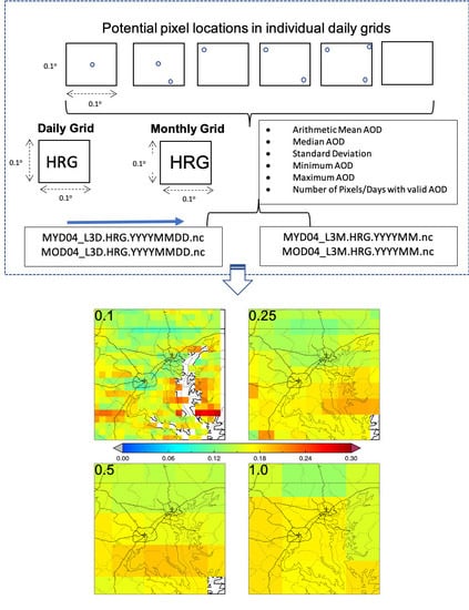
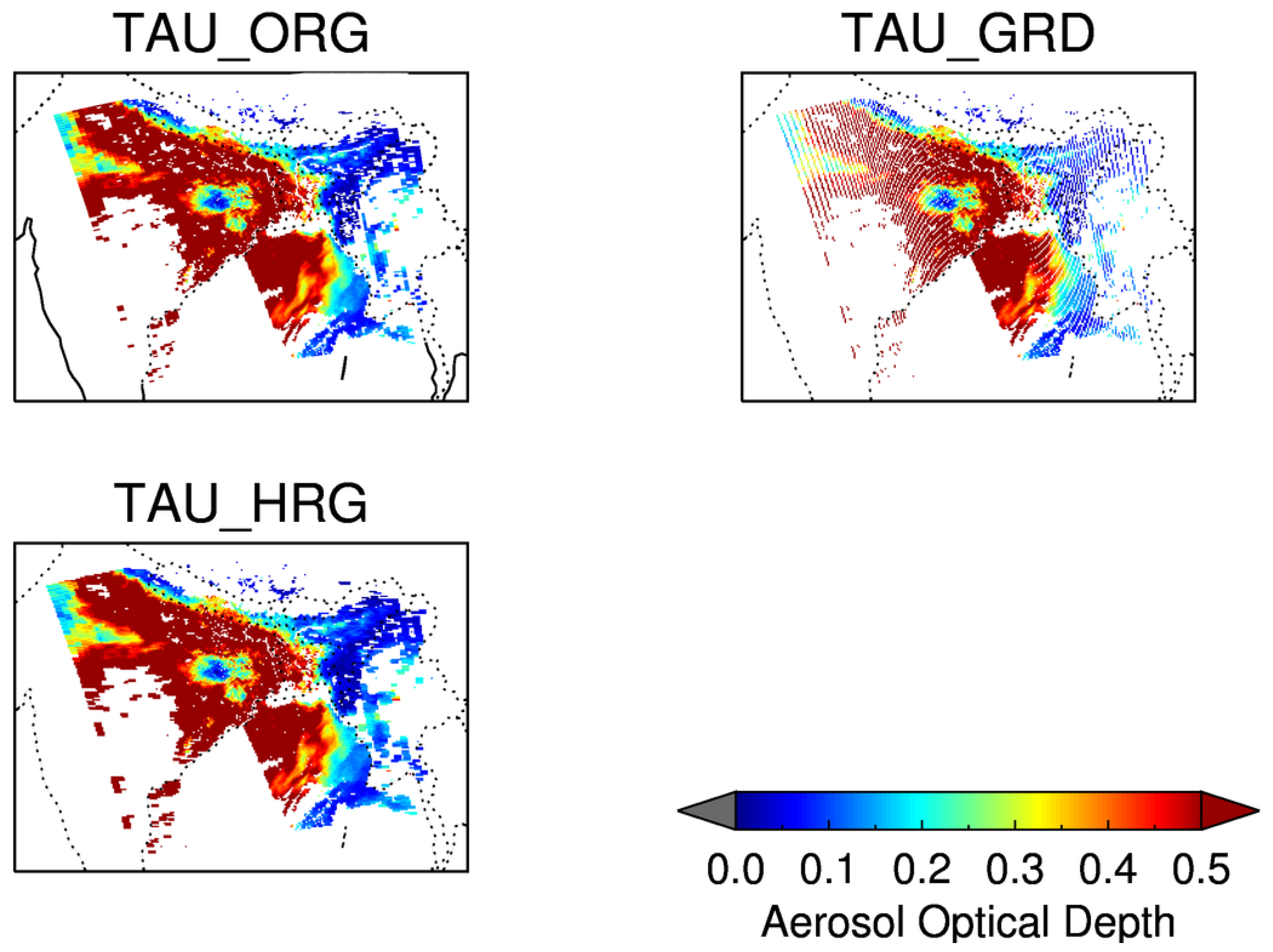
Figure 1 presents the flow chart of the data processing and schematic of potential grids with output variables and filenames. For every day, we accumulated all the 5-min granule files and then aggregate AOD values to a predefined fixed equal angle grid with a spatial resolution of 0.1 × 0.1 degree in latitude and longitude (hereafter called “high-resolution grid” (HRG)). The latitude/longitude tag associated with each retrieval in the granule represents the center of the retrieval. Whichever grid box contains that latitude/longitude mark will receive the AOD from that retrieval. Because the orbital path does not align with a north–south grid and the instrument is scanning side-to-side as the satellite progresses forward, there is distortion in the image when it is mapped to the Earth’s geoid. The distortion creates situations when more than one Level 2 retrieval will fall within the 0.1 × 0.1-degree grid box, creating the need to calculate an average value for the grid box. There are other situations when a 0.1 × 0.1-degree grid box will have no Level 2 retrievals within the box, even though the Level 2 product resolution is roughly the same size as the grid. As we move towards the edge of the swath (higher viewing angles), due to an increase in pixel size (by a factor of 2 to 5), several HRG grids will not receive any valid AOD values. The large pixel size at the edge can create artificial data gaps in HRG data at higher viewing angles. Therefore, we used a spatial filling method by calculating pixel size as a function of viewing angle and filled all the empty grids within the MODIS original pixel with the same value. Figure 2 shows an example of one of the MODIS 5-min granules mapped by three different methods: (a) the original mapping with pixels varying in size in an irregular array; (b) HRG data of regular equal angular size with no filling; (c) HGR with spatial filling. The empty grids (white color—no data) in Figure 2 show the data gaps when not considering the original pixel size in gridding the data. In contrast, the map in Figure 2 fills those gaps when spatial averaging is applied to account for the variation of pixel size as a function of viewing angle.
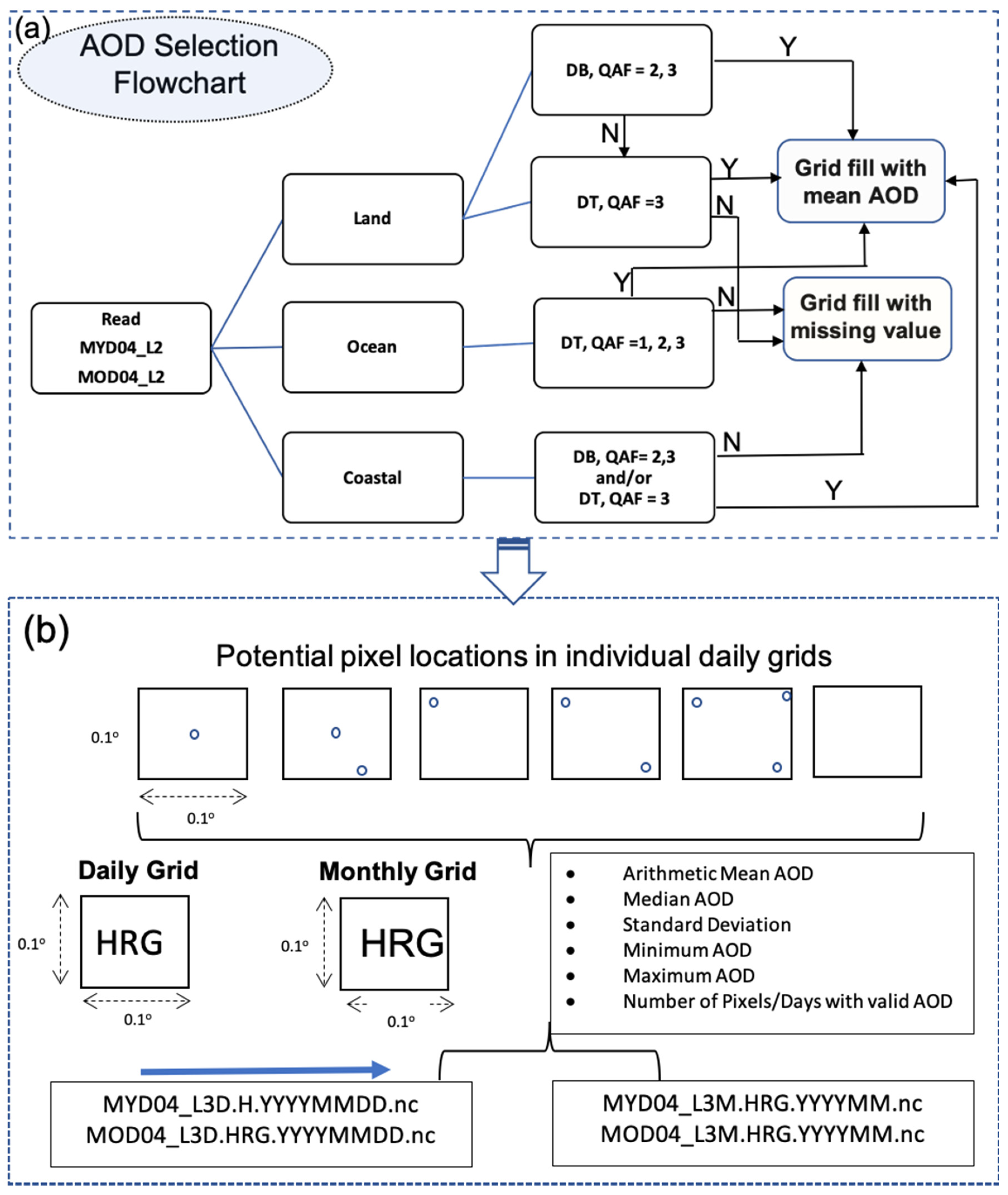
The following decision-making rules were applied to merge the Level 2 products at each fixed grid and generate daily global files of AOD statistics (Figure 1).
- Ocean grids use DT AOD with quality flags 1, 2, and 3.
- Land grids use DB AOD with quality flag 2 & 3. The remaining land grids were filled with DT AODs with quality flag 3.
- Coastal grids were filled with AODs from DT with QA = 3 and (or) DB with QA = 2, and 3. If both appropriate DT and DB retrievals are available, those retrievals are averaged.
- Grids with no available valid AODs were filled with a missing value of −1.000.
After accumulating AODs in each grid, statistics such as minimum (MIN), maximum (MAX), arithmetic mean (AVG), median (MED), standard deviation (STD), number of valid AOD pixels (PIX) are calculated and stored. In addition to these statistics, additional details such as information about algorithms, land, ocean, and coastal identifiers are saved in each file. After this exercise, we now have one single daily file for each MODIS sensor with data for the entire globe. Figure 1b provides a schematic showing some potential grid scenario and arrangement of available valid AODs and resulting grids with a list of available statistical parameters.
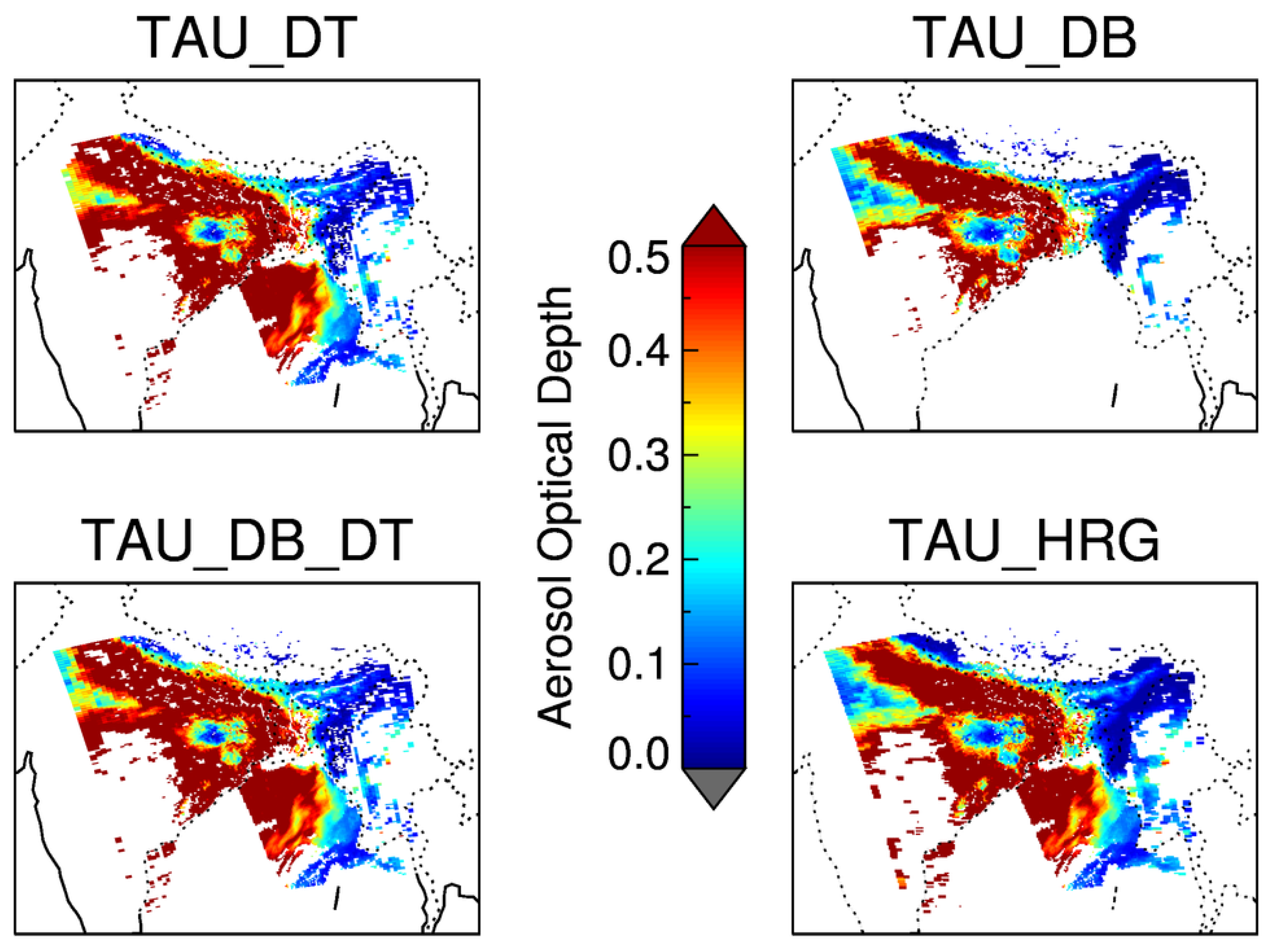
Figure 3 provides an example of the MODIS 5-min granule (same as shown in Figure 2) with different AOD SDSs mapped. Panels a and b in Figure 3 show the DT and DB AOD, respectively. Here it is important to note that the MODIS DB and DT algorithm teams already provide a merged AOD (Figure 3) at Level 2 (pixel data) based on quality flags and the Normalized Difference Vegetation Index (NDVI) threshold [8]. The algorithm team considers it the best estimated AOD values from the two algorithms. The downside of this merged AOD data is its reduced spatial coverage as compared to actual combined coverage by the two algorithms. The decision of algorithm selection in the operational merged product is based on the monthly mean climatology of NDVI, which forces certain areas of the Earth always to prefer one of the two algorithms. While in operation, both algorithms use real-time measurements for estimating surface reflectance, and that affects the quality and coverage of AODs retrieved by each algorithm. Therefore, the merging method adopted by the algorithm team is more conservative and preserves the selection of an individual algorithm for a certain type of surface even when the chosen algorithm is refraining from making retrievals in that particular situation. The merged product is forced to carry the “holes” in the spatial coverage of the selected algorithm that could otherwise have been filled in by the algorithm not chosen. This can be seen in the maps of Figure 3 over parts of the Indo Gangetic Plain, and north-east India where the DT algorithm produces AOD (Figure 3) with some data gaps (white color area on the map) in the middle of the aerosol plumes whereas the DB AOD (Figure 3) map has fewer data gaps. The operationally combined AOD (Figure 3) map shows most of the data gaps, as seen in the DT map (Figure 3), that could have been avoided if DB had been chosen for those locations. This is mainly due to the selection of DT over DB AODs over those particular areas based on the climatological NDVI values. Our current approach that we demonstrate in this paper uses the strength of each of the two algorithms and fills those gaps for the HRG data set (Figure 3) by removing NDVI filtering when combining the two AODs. In addition, the two algorithms handle AOD retrievals very differently in the presence of thick smoke and dust plumes. The DB algorithm is more successful in retrieving AODs in thick aerosol layers as compared to the DT algorithm, which is stricter in filtering out clouds. The DT algorithm also misses AOD over very bright urban surfaces under low aerosol loading and at certain viewing geometry. A recent global validation study [34] found that the DB product outperforms the DT product over land according to several validation metrics, including percent within expected uncertainty (%EE) and root mean square error (RMSE). The DB product also has more extensive global coverage over land as compared to DT. Therefore, in our approach, we aim to increase the daily spatial coverage while using the best of the two algorithms by applying a more dynamic AOD merging method.
2.4. Spatial and Temporal Coverage
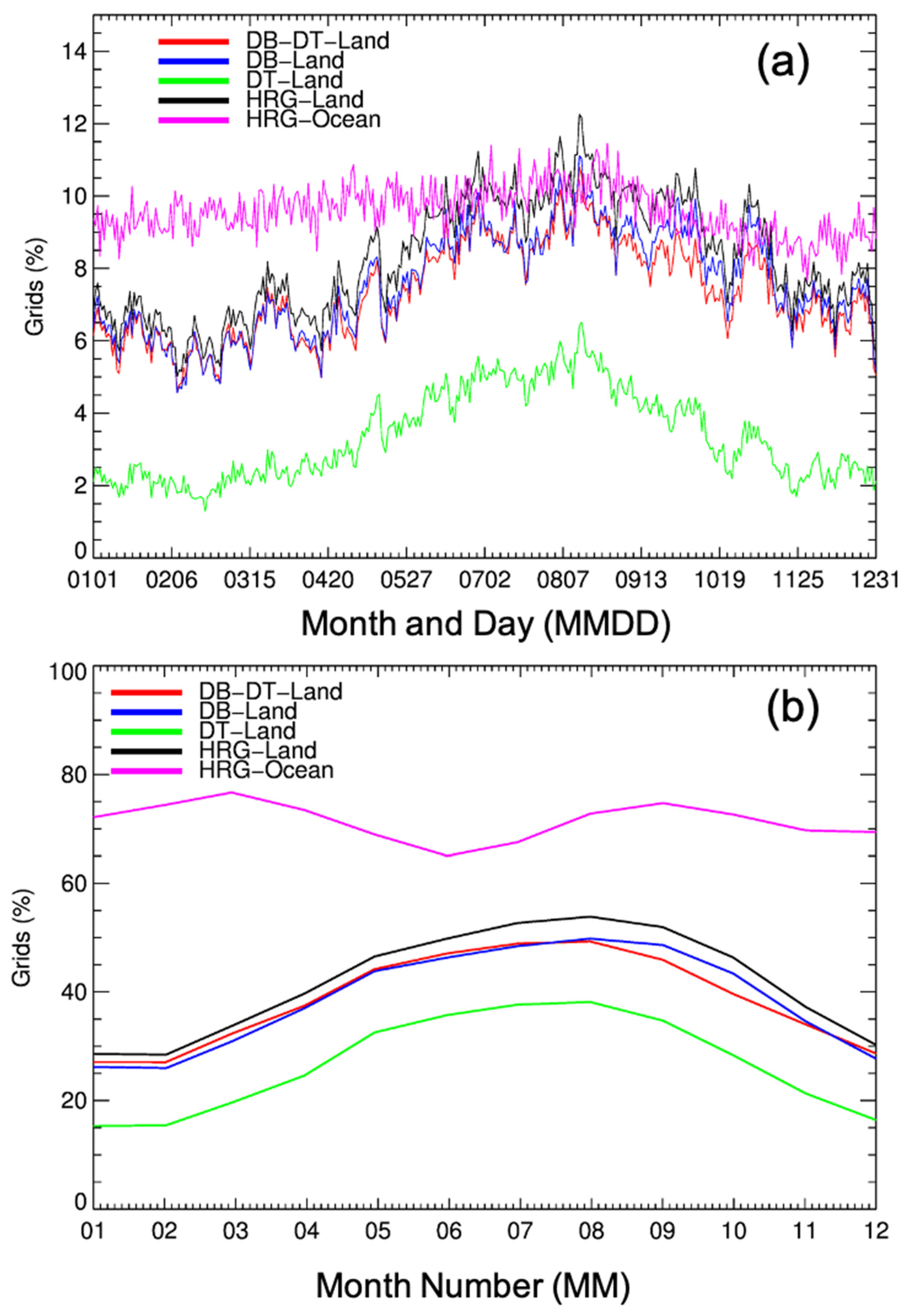
Figure 4a shows the daily percentage of available AOD product in the 0.1 × 0.1 grids over land and ocean in (calendar year) 2010 using (a) DT retrieved only, (b) DB retrieved only, (c) the operational DB–DT merged product, and (d) this approach (i.e., HRG). The percentages were calculated by divining number of grids with valid AOD by total number of grids individually for land and ocean. As noted earlier, over the ocean, we only have DT retrieved AODs; therefore, the magenta line in the figure represents both DT and HRG grids as they are the same. Over the ocean, the spatial coverage is highest during the northern hemisphere summer months and lower in winter months with an annual average of 9.6% grids with valid AODs on a given day. Over the land, it is clear that DT has the lowest spatial coverage (3.4%), and it increases for DB–DT (7.3%), DB (7.6%), and is highest for HRG (8.3%). The reasons for the lowest coverage by DT are its limitation to retrieve only over dark and vegetated surfaces. In contrast, the DB algorithm makes retrievals over both bright and dark surfaces over the land. Both the DB and DT algorithms do not make any retrievals over snow/ice and under cloudy conditions. The seasonal variability in spatial coverage is similar for all the retrieval combinations with lowest values being recorded in northern winter and the highest in northern summer months and most likely contributed to by the seasonality of snow/ice on the surface and cloud cover. The HRG provides the highest spatial coverage of AOD retrievals for daily analysis over global regions.
Daily gridded files were then used to create monthly means. We did not apply any additional quality control criteria while converting daily to monthly but simply averaged all available daily values for each grid within a given month. Note that this differs from the MODIS operational Level 3 monthly mean AOD at 1 × 1 degree resolution, which requires at least 3 days of data available for each grid. In addition to the average value, we provide other statistics such as the number of days for which AOD values are available, standard deviation, median, minimum, and maximum for each grid that can help users to further quality control the data suitable to address specific research or application needs.
Figure 4b shows the same information as Figure 4a but for the monthly data. The seasonal variability over land is the same as daily data, but over the ocean, the monthly mean availability shows less seasonal variability with a mean coverage of about 71.5%. The mean coverage over land for DT, DB–DT, DB, and HRG are 26.7%, 38.5%, 38.6%, and 41.6%, respectively.
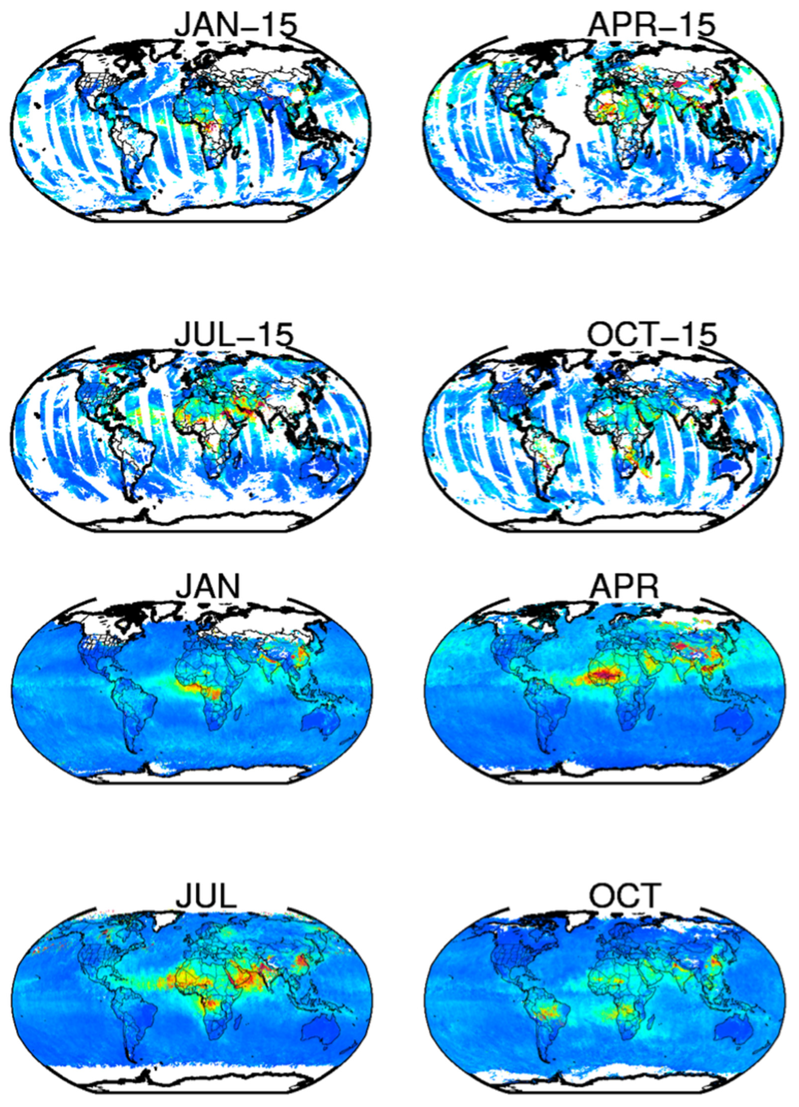
Figure 5 presents the daily and monthly converge of HRG AODs for MODIS-Aqua for the year 2010. The daily maps are produced for the 15th of four selected months (Jan, Apr, Jul, Oct) to represent seasonal differences in coverage, mainly due to changes in cloud, snow, and ice coverage. The continuous white space in the daily AOD maps are satellite orbital gaps; white spaces over the ocean are either sun-glint regions where high ocean reflectivity does not allow AOD retrieval in the current DT algorithm, or a region with cloud/snow/ice. The monthly maps were produced for the same four selected months. The monthly maps provide better global coverage where data gaps are mostly related to snow/ice on the surface due to seasonal changes at the different latitudes of both sides of the tropics.
3. Results
3.1. Validation with AERONET
3.1.1. Spatial and Temporal Collocation and Statistical Analysis
The HRG daily data were collocated using a spatio–temporal technique [33,38] used for the MODIS validation exercise [31] over global AERONET stations. We revised the method slightly to accommodate gridded data instead of swath data. In this method, AODs from 3 × 3 grids centered over the AERONET location were averaged. This is equivalent to about a 30 × 30 km2 area. To represent the same air mass for the comparison, AERONET AODs were averaged over ±0.5 h to the satellite overpass time over the particular AERONET station. To be consistent with previous validation studies [3,31,33], we retained the collocated data sets only when there were at least three MODIS pixels (out of possible nine) and two AERONET measurements (out of 2–6). We used 15+ years of MODIS data from 2001–2018 in this validation exercise. The validation was performed separately for MODIS-Terra and MODIS-Aqua. The collocated validation data set consists of 834 AERONET stations with 239,340 AOD pairs for MODIS-Aqua and 288,883 pairs for MODIS-Terra satellites. To analyze the validation results and uncertainties, the following statistical parameters were calculated similarly to those used in Gupta et al. [33]:
Root mean square was estimated using the equation:
The error of estimation, as given by the MODIS science team [32] through validation exercises, is presented in Equation (3).
It is customary to represent the percentage of retrievals, which falls within the envelope of EE and AERONET AODs, as given by Equation (4).
Here
- AODAERO: Aerosol Optical Depth at 0.55 µm from AERONET
- AODMODIS: Aerosol Optical Depth at 0.55 µm from MODIS
Other than these parameters, the linear correlation coefficient and the number of data points and regression coefficients were also used to interpret the relationship between different AODs.
3.1.2. Global Validation
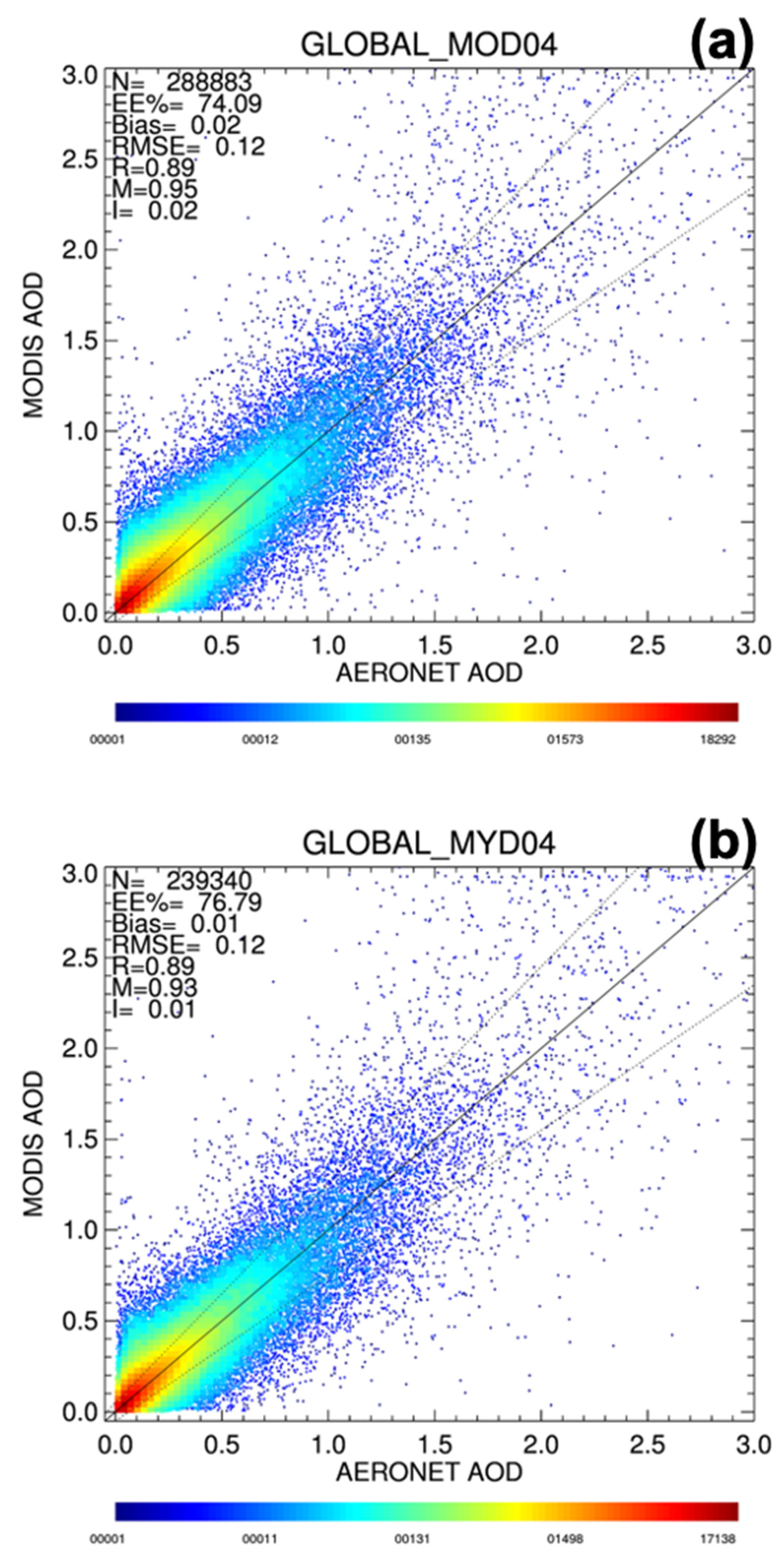
Figure 6 presents the density scatter plot of the AODs from AERONET and those from HRG. The top panels are for Terra, and bottom panels are for Aqua. The figure also provides all the statistics associated with these figures, including the number of data points (N), slope (M), Intercept (I), RMSE, EE%, and correlation coefficients (R). The correlation between AODMODIS and AODAERO remains the same (0.89) between MODIS-Terra and MODIS-Aqua satellites. Wei et al. [34] used much smaller data sets over global locations and reported correlation values of 0.92, 0.90, and 0.91 for DT, DB, and the operational DT/DB merge from MODIS-Terra. The RMSE for MODIS-Terra and MODIS-Aqua is 0.12 and very similar to the previously reported value of 0.11 for both DB and DT validation [34]. The number of retrievals within expected errors as defined by EE% are ~77% and ~74%, which are very close to earlier reported values of 71%, 76%, and 72% for DT, DB, the operational merged product, respectively, for MODIS-Aqua and MODIS-Terra. Overall, MODIS-Aqua performed better than MODIS-Terra in this study, which is also consistent with previously reported findings [3,32,33,39].
3.1.3. Regional Validation
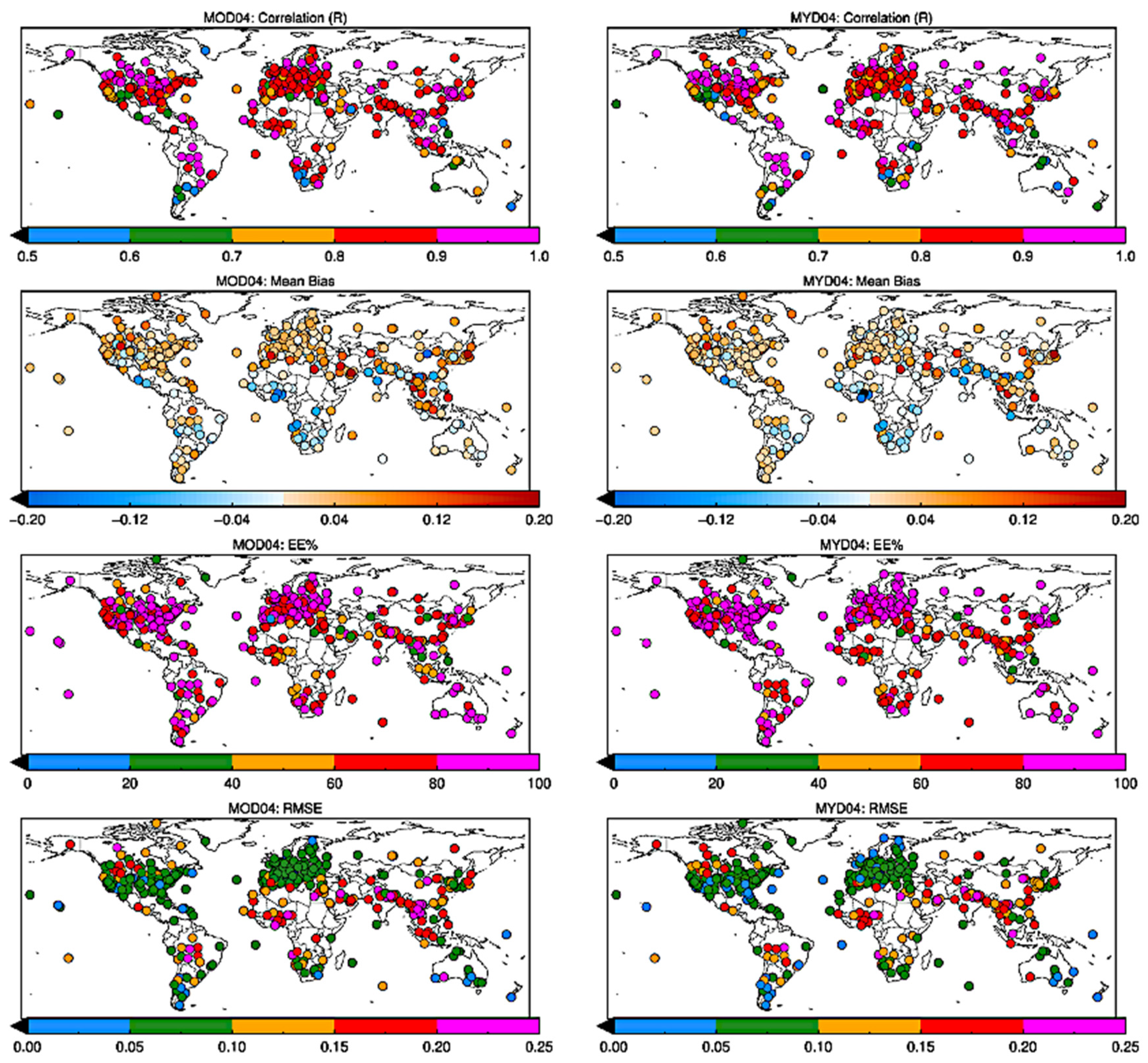
Atmospheric aerosols have different regional sources, and their composition varies in different parts of the world. In addition, surface reflectance varies widely, introducing different levels of uncertainty into a global aerosol retrieval. Many research studies focus on the regional impacts of aerosols on climate and air quality; therefore, it is vital to know the regional validation parameters of retrieved AODs. Figure 7 presents the correlation coefficient, mean bias, EE%, and RMSE calculated from the MODIS-AERONET collocation scatterplots at individual AERONET station for both MODIS-Terra and MODIS-Aqua.
We only considered AERONET stations with a sufficient number of collocated pairs (>100) for the individual station analysis. Combining both Terra and Aqua data shows that about 30% of the stations have correlation values greater than 0.9, and 80% of stations have a value of R greater than 0.8. We found only about 10% of stations with R values less than 0.5. Further examination shows that a majority of stations with R < 0.5 are located either at high elevation or coastal sites. The poor performance over these locations is expected and consistent with previous validation findings [3,32,33,39].
The mean bias (Figure 7) for 75% of the stations falls within ±0.05 and 93% stations have bias within ±0.1, with only a few stations (7%) with larger bias values (>|0.1|). These sites were not necessarily the same as those with low correlations. Some of these sites were located in highly polluted regions of the world with a complex mixture of aerosols such as tropical Africa, China, India, and Mexico City. The spatial distribution of biases found in this study is consistent with those reported for the DB–DT combined validation study [34].
The expected error (EE%) is defined differently for each algorithm, land, and ocean separately. Here for consistency, we used a fixed definition as defined by Equations (3) and (4). This parameter allows us to find the percentages of retrievals which falls within a predefined error envelope. About 76% of AERONET stations have MODIS HRG AOD matching AERONET observations within EE% values more than 66% of the time, which satisfies the validation criteria as set up by algorithm teams, and 60% of stations match AERONET within EE% values more than 75% of the time. Only about 7% of stations demonstrate a poor ability to retrieve within EE % values (<50% of the time). The spatial distribution of EE% matched with those reported in Wei et al., 2019, with high values in the US and Europe and lower values in Asia.
The global RMSE is about 0.12 and varies between 0.0 and 0.25 from station to station. The number of stations with RMSE < 0.1 is about 65%, with only 10% of stations having values of RMSE > 0.2. AERONET stations with high RMSE are aligned with those having high aerosol loading and high biases as expected.
3.1.4. Error Dependencies
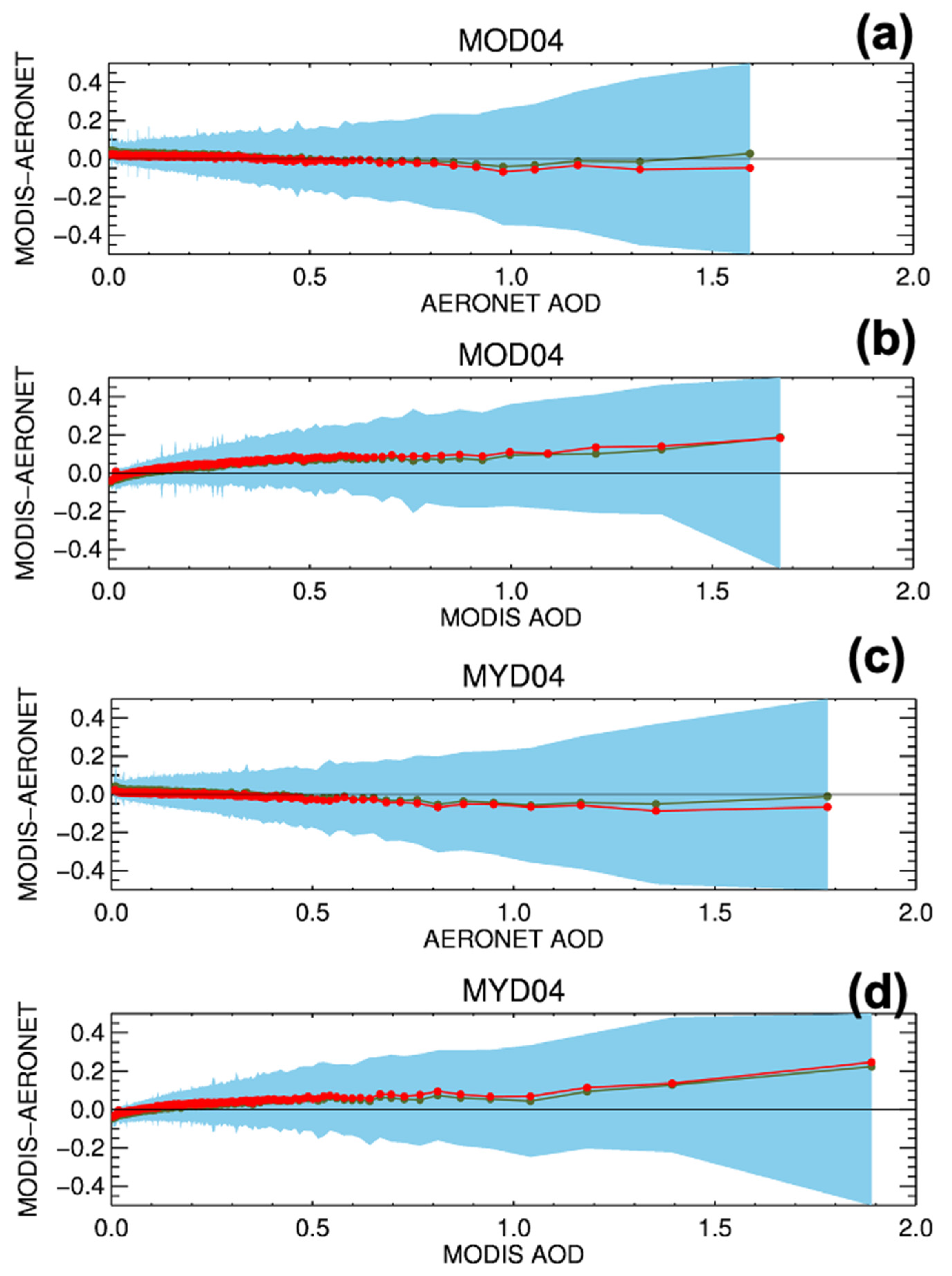
The biases calculated for Level 2 AOD retrievals are often defined with respect to ground truth measurements (i.e., AERONET) and considered as diagnostic errors [32,33]. Independent validations studies [31,32,33,34] have shown that various error parameters (Section 3.2) depend on atmospheric aerosol loading, types of aerosols, surface properties (i.e., land cover, reflectance), cloud cover, and sun-satellite viewing geometry. In this study, we validated gridded products, which do not carry over all the sun-satellite geometry from the original L2 product. Therefore, we evaluated errors as a function of AERONET AODs (i.e., diagnostic) and retrieved AODs (prognostic). We followed the method of collocation and estimating bias, as described in Gupta et al., [33], to analyze diagnostic and prognostic errors in gridded AODs. Figure 8 shows the results of this analysis as a function of both true AODs, as measured by AERONET (Figure 8a,c) and the HRG AODs as retrieved by MODIS (Figure 8b,d). The red dots and line on the plot show the mean of each bin with an equal number of data points, whereas green color represents the median of the same bins. The shaded area represents one standard deviation for each bin. The bias in gridded AODs depends very little on the actual AODs. There is some suggestion of positive biases for lower AODs (<0.5) and negative biases for higher AODs (>0.5), but overall the differences are flat.
The prognostic error is more useful for the end-user as it is defined with respect to retrieved AODs (i.e., MODIS) rather than the reference AODs (i.e., AERONET). This is important as AERONET AODs are not available everywhere, and only retrieved AODs are available in routine processing. Figure 6 show bias results as a function of gridded AODs, which demonstrate systematic behavior with a low bias for low AOD range and increase with an increase in retrieved AOD values. For retrieved AOD < 0.10, the mean differences between MODIS and AERONET are negative. This indicates that a high value of retrieved AOD has a greater probability of being too high than too low, and a low value of retrieved AOD has a greater probability of being too low than too high. These results are consistent with other published research [33], and expected regimes of AODs are more sensitive to aerosol properties, whereas low AOD regimes are more sensitive to surface properties. The bias in the HRG AOD data can be quantified by −0.01 + 0.18 × AODmod and −0.01 + 0.15*AODmod for MODIS-Terra & MODIS-Aqua, respectively. Therefore, MODIS-Terra AODs are slightly biased higher as compared to MODIS-Aqua. This Terra-Aqua bias is expected from the previous analysis and may be explained in part by calibration differences [39]. The bias equations can be further used to make bias correction of individual gridded AODs on a daily scale.
3.2. Applications Examples
3.2.1. Spatial Gradient at Local and Regional Scales
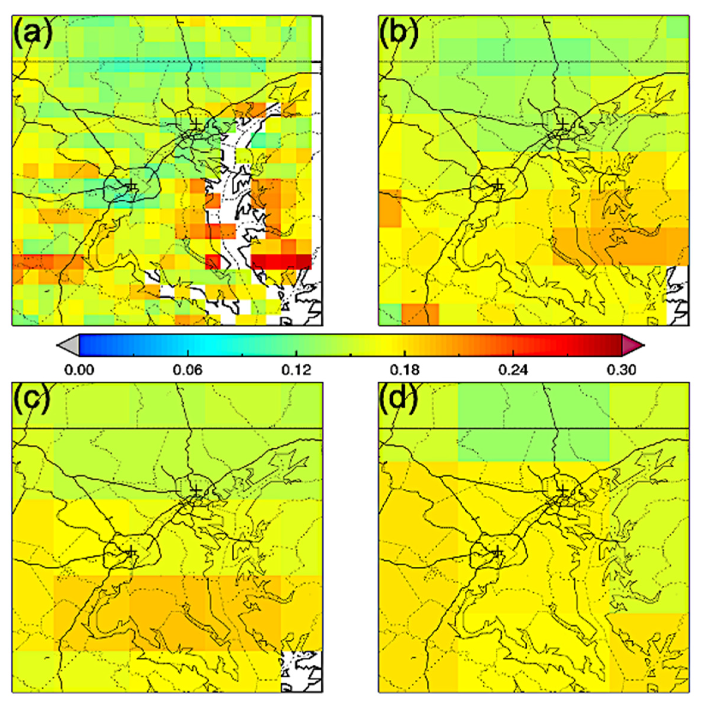
Figure 9 shows the spatial distribution of July 2010 monthly mean MODIS AOD in a 2 × 2 degree box around the Washington Metro Area (WMA). Figure 9a was created using high-resolution gridded (i.e., HRG) data at 0.1 × 0.1 degree, whereas the other three panels show the same data sampled at coarser resolutions of 0.25, 0.5, and 1 degree. The figure shows a spatial gradient of aerosol loading across this local area, with higher AOD concentrated near the Chesapeake Bay and not in the urban centers of Washington DC and Baltimore. This gradient starts disappearing as the data are re-gridded to coarser grids. Obviously, existing Level 3 products at 1-degree resolution are inadequate to characterize the aerosol patterns at this spatial scale. A key element to consider in Figure 9 is that the spatial plot of monthly mean AOD is much easier to calculate from daily values now that Level 2 data has been stored in a grid. The new gridded data should encourage similar studies in other parts of the world with minimal data processing and significantly quicker analysis than if using orbital Level 2 data. The map still could suffer from an uneven sampling of the AOD during the month, as some regions may be cloudier than others with specific grids reporting fill values, creating a composite of AOD constructed from different days in different parts of the 2 × 2 degree box. Thus, the new HRG data provide an excellent new tool for the community, but critical scientific analysis is still required to interpret the results accurately.
3.2.2. Long Range Dust Transport over the Atlantic Ocean
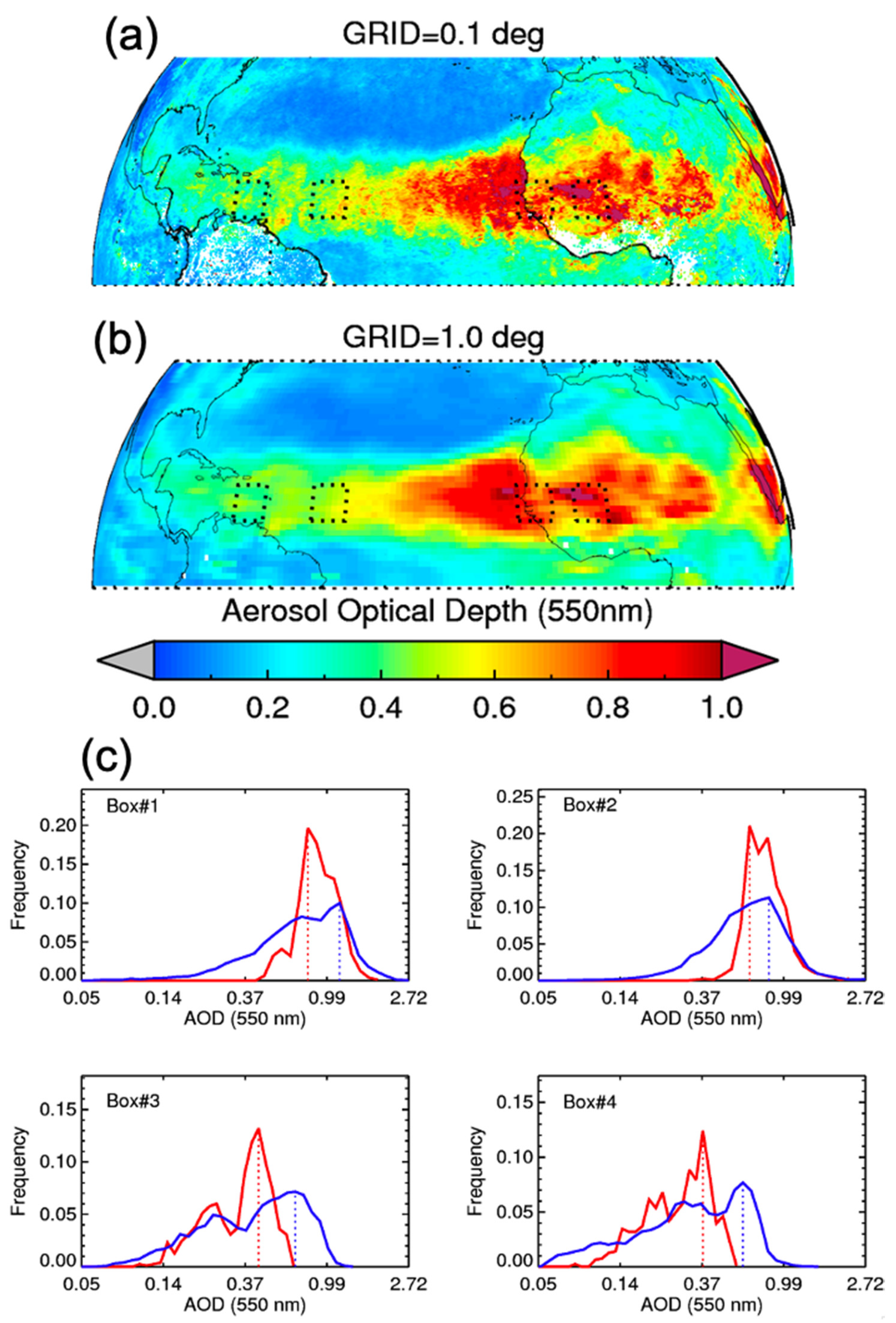
Satellite data have long been used to monitor and track long-range transport of aerosols across regions. Aerosols from biomass burning [40,41,42,43], dust storms [23,44], and volcanic eruption [45] are some of the most popular types of transport that happen at various temporal and spatial scales. Figure 10 shows an example of dust transport across the Atlantic Ocean in June–July 2018. The dust storm originated over the Saharan desert around June 18 and, in about 6 days, reached the coast of South America and was further transported to various parts of Central America and the southeastern coast of the USA. During the remaining month of June and until early July, the dust transport continued. Figure 10a shows the 16-day composite mean AOD using the HRG data, whereas Figure 10b shows the same data but sampled at the coarser resolution grid (CRG) of a 1 × 1 degree. The two maps show very high values of AOD over North Africa and the transport path over the Atlantic Ocean. Overall the two maps show similar spatial features of the AOD, but zooming into smaller areas in the path of the dust plume makes apparent a significant structure in the HRG AODs as compared to coarse resolution data. To further investigate the observed AOD values during the dust storm, we analyzed histograms of AODs over four selected, 10 × 10 degree boxes at the source, and along the path of dust transport.
We used the data at HRG and CRG to examine the observed histograms of AODs. Figure 10c shows the normalized frequency of AODs for 16 days at HRG (blue line) and CRG (red line) in four selected boxes. The box boundaries are shown on the maps. The common features of the AOD histograms among the four boxes are (a) the HRG histogram is much wider than the CRG, meaning that the HRG AODs demonstrate a larger range of AODs observed in each box; (b) the peak of the histogram is shifted for HRG towards higher AOD values. Not only does the range of AOD depend on resolution, but also the mean. Relying on the current operational Level 3 CRG product for calculating the severity of a major aerosol event, such as this dust transport, will underestimate the overall loading of the event. This will have consequences for estimations of the event’s radiative effect, mass flux, and deposition.
3.2.3. Long-Term Aerosol Trends
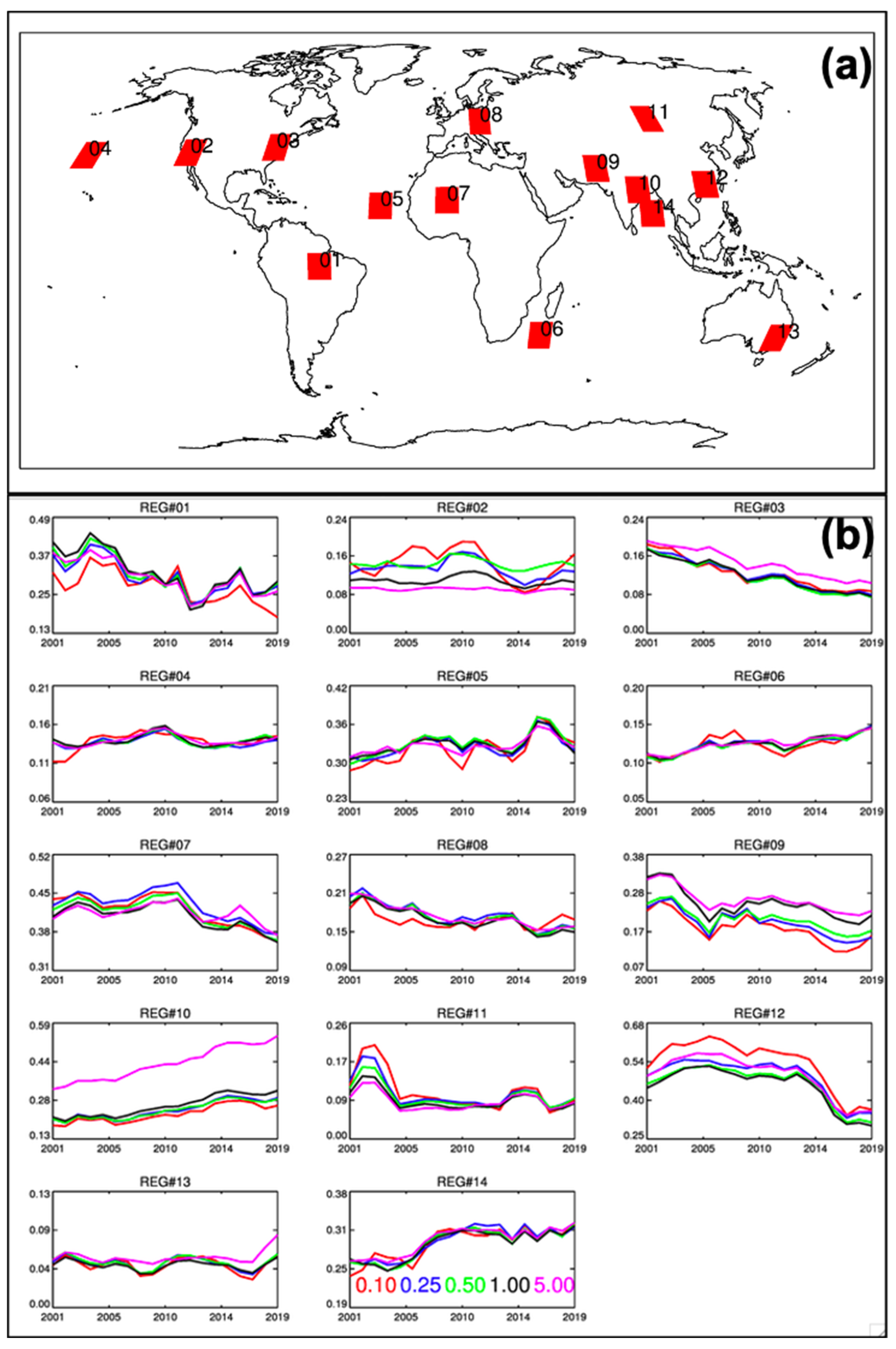
The aerosol product record from MODIS-Terra spans about 20 years. Over the years, several studies [46,47,48] have used this long time series to demonstrate aerosol trends at local, regional, and global scales. The high-resolution gridded data should enable more studies at finer spatial scales. Here we demonstrate the application by comparing trends between MODIS-Terra over 14 regions of the world (Figure 11). The regions were selected to cover various types of surface and aerosol and cover, as shown in Figure 11a. Figure 11b shows the yearly mean AOD from 2001 for varying spatial averaging. Each line in the timeseries represents spatial averaging window varying from 0.1 × 0.1, 0.25 × 0.25, 0.5 × 0.5, 1.0 × 1.0, and 5.0 × 5.0 degrees. Here the purpose was not to discuss the regional trends and geophysical reasons for these trends but to demonstrate the application of the HRG data set and compare and contrast with CRG data sets.
Regions number 1 (Amazonia), 3 (eastern US), 8 (Europe), and 12 (China) show significant decreasing trends in AODs over the years. Similarly, regions number 6 (Indian Ocean), 10 (Northern India), and 14 (Bay of Bengal) demonstrate increasing trends. Other parts of the world shown in the figure either show very weak trends or no trends. The spatial resolution of the product does not affect the overall sign of the trends noted above. However, the spatial resolution does affect the mean values and interannual variability of the AOD in specific locations. The aerosols are spatially more homogeneous over the ocean as compared to the land, and the more spatially homogeneous, the less effect varying spatial resolution will have on the mean values of the box. The variability in mean AOD with varying spatial resolution is minimal for the boxes (4, 5, 6, and 14) over the ocean. The boxes showing the most effect of spatial resolution are box 2 (western US) and boxes 9, 10 and 12 in Asia. In the box 2 the AOD timeseries for larger spatial resolution (i.e., 1, 5 degree) is almost flat with minimal year to year variability. As we reduce the grid size (i.e., 0.5, 0.25, 0.1 degree), the AOD starts showing some year to year variability. The region experiences significant biomass burning almost every year. This, coupled with complex topography and a mixture of urban and rural areas, often produces high spatial heterogeneity in the aerosol loading. Performing trend estimation using CRG data may not bring out the changes at local scales, as demonstrated in this example. Similarly, boxes 9, 10, and 12 in Asia show a significant difference in the magnitude of the annual mean in each 5-degree box, depending on the spatial resolution. These regions in Asia are considered to be exceptionally polluted areas with high population density having locally intense pollution sources with strong seasonality. These are factors that combine to create an inhomogeneous aerosol mixture that requires finer spatial resolution to characterize the interannual variability accurately.
4. Data Access and Visualization
The high-resolution product was developed while keeping in mind the needs of end-users who may have relatively little experience in handling large data volumes and limited computing resources. Acquiring, reading, and analyzing Level 2 aerosols data for any application requires a significant amount of time and computing resources. The MODIS Level 2 aerosol product has about 150 files per day with a total data volume of about 385 Mb, which translates to about 140 GB per year, and 2.8 TB for 20 years of records. This volume of data storage and processing can take a significant amount of computing and human resources. The HRG data are provided in daily and monthly files; one file contains data for the entire globe. Each daily file size is about 7.5 Mb, and that translates into 2.7 GB per year and 54 GB for the 20 year records. The data are stored in the NetCDF file format, which is more common than the Level 2 data format (i.e., HDF). The reduced data volume (by about factor of 50) and easy to use format will encourage greater usage. Currently, we provide all the monthly data files, python scripts, and readme files through an open server. The files can be accessed from the following website (https://www.nsstc.uah.edu/data/sundar/MODIS_AOD_L3_HRG). We are in the process of providing daily data from the same website in the near future. The new data set becomes even more powerful when combined with an online visualization tool for viewing validation results over global AERONET locations that can be accessed from the same link. Several end-user groups have already been using these data sets to analyze various air quality and climate applications [49].
5. Discussion and Conclusions
MODIS aboard NASA’s Earth Observing Satellites has been providing state-of-art multispectral measurements with a moderate spatial resolution (0.25 to 1 km) for over two decades. Historically, operational Level 2 aerosol products are available at a nominal 10 km spatial resolution. The quantitative use of Level 2 aerosol data requires a significant level of expertise in aerosol remote sensing, computer programming, and computing resources. The Level 3 operational gridded aerosol data from MODIS is available since the beginning of the mission but at much coarser spatial resolution (1 × 1 deg). NASA also provides state-of-art online visualization and analyzing tools to explore Level 3 gridded data sets. The coarser resolution of aerosol data limits its applications to large regional to global scale research and analysis. Initially, the aerosol products were developed to address climate change research and to evaluate global climate models where coarser resolution was adequate. However, over the years, the air quality community has utilized aerosol data sets and applied it to address varying air quality research and application issues at varying temporal and spatial scales.
We developed a high-resolution gridded aerosol data set at daily and monthly time scales from both MODIS-Terra and MODIS-Aqua. The gridded data sets were validated against ground measurements over global locations, and errors were characterized. The new gridded data match ground truth equally well with existing MODIS Deep Blue and Dark Target aerosol products, and in some cases, perform better and allow for greater availability of AOD products. We have also shown some example applications to demonstrate the use of this gridded data product. Finally, our visualization and data download tools will help end-user to access and analyze the data sets efficiently.
Author Contributions
Conceptualization, P.G.; software, P.G.; validation, P.G.; formal analysis, P.G., L.A.R., F.P.; writing—original draft preparation, P.G.; writing—review and editing, L.A.R., F.P., S.A.C.; visualization, P.G., L.A.R., F.P.; supervision, R.C.L.; project administration, P.G.; funding acquisition, P.G., R.C.L., L.A.R., F.P. All authors have read and agreed to the published version of the manuscript.
Funding
This research was supported by the NASA ROSES program NNH17ZDA001N-TASNPP: The Science of Terra, Aqua, and Suomi NPP.
Acknowledgments
Pawan Gupta, Lorraine Remer, Robert Levy, and Falguni Patadia were partially supported by the NASA ROSES program NNH17ZDA001N-TASNPP: The Science of Terra, Aqua, and Suomi NPP. The MODIS Aerosol Optical Depth data sets were acquired from the Level −1 and Atmosphere Archive & Distribution System (LAADS) Distributed Active Archive Center (DAAC), located in the Goddard Space Flight Center in Greenbelt, Maryland (https://ladsweb.nascom.nasa.gov/). We also like to thank Jashwanth Reddy Tupili (UAH) for developing python scripts to read and map the data sets.
Conflicts of Interest
The authors declare no conflict of interest.
References
- Hsu, N.C.; Tsay, S.; King, M.D.; Member, S.; Herman, J.R. Aerosol Properties over Bright-Reflecting Source Regions. IEEE Trans. Geosci. Remote Sens. 2004, 42, 557–569. [Google Scholar] [CrossRef]
- Hsu, N.C.; Jeong, M.J.; Bettenhausen, C.; Sayer, A.M.; Hansell, R.; Seftor, C.S.; Huang, J.; Tsay, S.C. Enhanced Deep Blue aerosol retrieval algorithm: The second generation. J. Geophys. Res. Atmos. 2013, 118, 9296–9315. [Google Scholar] [CrossRef]
- Sayer, A.M.; Hsu, N.C.; Bettenhausen, C.; Jeong, M.J. Validation and uncertainty estimates for MODIS Collection 6 deep Blue aerosol data. J. Geophys. Res. Atmos. 2013, 118, 7864–7872. [Google Scholar] [CrossRef] [Green Version]
- Remer, L.A.; Kaufman, Y.J.; Tanr, D.; Mattoo, S.; Chu, D.A.; Martins, J.V.; Li, R.-R.; Ichoku, C.; Levy, R.C.; Kleidman, R.G.; et al. The MODIS aerosol algorithm, products and validation. J. Atmos. Sci. 2005, 62, 947–973. [Google Scholar] [CrossRef] [Green Version]
- Levy, R.C.; Remer, L.A.; Mattoo, S.; Vermote, E.F.; Kaufman, Y.J. Second-generation operational algorithm: Retrieval of aerosol properties over land from inversion of Moderate Resolution Imaging Spectroradiometer spectral reflectance. J. Geophys. Res. Atmos. 2007, 112, 1–21. [Google Scholar] [CrossRef] [Green Version]
- Levy, R.C.; Mattoo, S.; Munchak, L.A.; Remer, L.A.; Sayer, A.M.; Patadia, F.; Hsu, N.C. The Collection 6 MODIS aerosol products over land and ocean. Atmos. Meas. Tech. 2013, 6, 2989–3034. [Google Scholar] [CrossRef] [Green Version]
- Gupta, P.; Levy, R.C.; Mattoo, S.; Remer, L.A.; Munchak, L.A. A surface reflectance scheme for retrieving aerosol optical depth over urban surfaces in MODIS Dark Target retrieval algorithm. Atmos. Meas. Tech. 2016, 9, 3293–3308. [Google Scholar] [CrossRef] [Green Version]
- Sayer, A.M.; Munchak, L.A.; Hsu, N.C.; Levy, R.C.; Bettenhausen, C.; Jeong, M. MODIS Collection 6 aerosol products: Comparison between Aqua’s e-Deep Blue, Dark Target, and merged data sets, and usage recommendations. J. Geophys. Res. Atmos. 2014, 119, 13965–13989. [Google Scholar] [CrossRef]
- Christopher, S.A.; Zhang, J. Shortwave aerosol radiative forcing from MODIS and CERES observations over the oceans. Geophys. Res. Lett. 2002, 29, 6-1–6-4. [Google Scholar] [CrossRef] [Green Version]
- Yu, H.; Dickinson, R.E.; Chin, M.; Kaufman, Y.J.; Zhou, M.; Zhou, L.; Tian, Y.; Dubovik, O.; Holben, B.N. Direct radiative effect of aerosols as determined from a combination of MODIS retrievals and GOCART simulations. J. Geophys. Res. 2004, 109, D03206. [Google Scholar] [CrossRef] [Green Version]
- Yu, H.; Kaufman, Y.J.; Chin, M.; Feingold, G.; Remer, L.A.; Anderson, T.L.; Balkanski, Y.; Bellouin, N.; Boucher, O.; Christopher, S.; et al. A review of measurement-based assessment of the aerosol direct radiative effect and forcing. Atmos. Chem. Phys. 2006, 6, 613–666. [Google Scholar] [CrossRef] [Green Version]
- Zhang, J.; Christopher, S.A.; Remer, L.A.; Kaufman, Y.J. Shortwave aerosol radiative forcing over cloud-free oceans from Terra: 2. Seasonal and global distributions. J. Geophys. Res. 2005, 110, D10S24. [Google Scholar] [CrossRef] [Green Version]
- Kaufman, Y.; Tanr, D.; Boucher, O. A satellite view of aerosols in the climate system. Nature 2002, 419, 215–223. [Google Scholar] [CrossRef] [PubMed]
- Bellouin, N.; Boucher, O.; Haywood, J.; Reddy, M.S. Global estimate of aerosol direct radiative forcing from satellite measurements. Nature 2005, 438, 1138–1141. [Google Scholar] [CrossRef]
- Kinne, S.; Lohmann, U.; Feichter, J.; Schulz, M.; Timmreck, C.; Ghan, S.; Easter, R.; Chin, M.; Ginouz, P.; Takemura, T.; et al. Monthly averages of aerosol properties: A global comparison among models, satellite data, and AERONET ground data. J. Geophys. Res. 2003, 108, 4634. [Google Scholar] [CrossRef]
- Koren, I.; Kaufman, Y.J.; Remer, L.A.; Martins, J.V. Measurement of the effect of Amazon smoke on the inhibition of cloud formation. Science 2004, 303, 1342–1345. [Google Scholar] [CrossRef] [Green Version]
- Koren, I.; Remer, L.A.; Altaratz, O.; Martins, J.V.; Davidi, A. Aerosol-induced changes of convective cloud anvils produce strong climate warming. Atmos. Chem. Physics 2010, 10, 5001–5010. [Google Scholar] [CrossRef] [Green Version]
- Kaufman, Y.J.; Remer, L.A.; Tanr, D.; Li, R.-R.; Kleidman, R.; Mattoo, S.; Levy, R.C.; Eck, T.F.; Holben, B.N.; Ichoku, C.; et al. A critical examination of the residual cloud contamination and diurnal sampling effects on MODIS estimates of aerosol over ocean. IEEE Trans. Geosci. Rem. Sens. 2005, 43, 2886–2897. [Google Scholar] [CrossRef]
- Myhre, G.; Stordal, F.; Johnsrud, M.; Kaufman, Y.J.; Rosenfeld, D.; Storelvmo, T.; Kristjansson, J.E.; Berntsen, T.K.; Myhre, A.; Isaksen, I.S.A. Aerosol-cloud interaction inferred from MODIS satellite data and global aerosol models. Atmos. Chem. Phys. 2007, 7, 3081–3101. [Google Scholar] [CrossRef] [Green Version]
- Kaufman, Y.J.; Koren, I.; Remer, L.A.; Tanr, D.; Ginoux, P.; Fan, S. Dust transport and deposition observed from the Terra-Moderate Resolution Imaging Spectroradiometer (MODIS) spacecraft over the Atlantic Ocean. J. Geophys. Res. 2005, 110, D10S12. [Google Scholar] [CrossRef] [Green Version]
- Stohl, A.; Berg, T.; Burkhart, J.F.; Fjǽraa, A.M.; Forster, C.; Herber, A.; Hov, Ø.; Lunder, C.; McMillan, W.W.; Oltmans, S.; et al. Arctic smoke record air pollution levels in the European Arctic during a period of abnormal warmth, due to agricultural fires in eastern Europe. Atmos. Chem. Phys. 2007, 7, 511–534. [Google Scholar] [CrossRef] [Green Version]
- Yu, H.; Remer, L.A.; Chin, M.; Bian, H.-S.; Tan, Q.; Yuan, T.; Zhang, Y. Aerosols from Overseas Rival Domestic Emissions over North America. Science 2012, 337, 566–569. [Google Scholar] [CrossRef] [PubMed]
- Yu, H.; Tan, Q.; Chin, M.; Remer, L.A.; Kahn, R.A.; Bian, H.; Kim, D.; Zhang, Z.; Yuan, T.; Omar, A.; et al. Estimates of African Dust Deposition Along the Trans-Atlantic Transit Using the Decadelong Record of Aerosol Measurements from CALIOP, MODIS, MISR, and IASI. J. Geophys. Res. Atmos. 2019, 124, 7975–7996. [Google Scholar] [CrossRef] [PubMed]
- Wang, J.; Christopher, S.A. Intercomparison between satellite-derived aerosol optical thickness and PM2. 5 mass: Implications for air quality studies. Geophys. Res. Lett. 2003, 30, 2095. [Google Scholar] [CrossRef]
- Gupta, P.; Christopher, S.A. Particulate matter air quality assessment using integrated surface, satellite, and meteorological products: Multiple regression approach. J. Geophys. Res. 2009, 114, D14205. [Google Scholar] [CrossRef] [Green Version]
- Van Donkelaar, A.; Martin, R.V.; Brauer, M.; Kahn, R.; Levy, R.; Verduzco, C.; Villeneuve, P.J. Global estimates of ambient fine particulate matter concentrations from satellite-based aerosol optical depth: Development and application. Environ. Health Persp. 2010, 118, 847–855. [Google Scholar] [CrossRef] [Green Version]
- Van Donkelaar, A.; Martin, R.V.; Brauer, M.; Hsu, N.C.; Kahn, R.A.; Levy, R.C.; Lyapustin, A.; Sayer, A.M.; Winker, D.M. Global estimates of fine particulate matter using a combined geophysical-statistical method with information from satellites, models, and monitors. Environ. Sci. Technol. 2016, 50, 3762–3772. [Google Scholar] [CrossRef]
- Duncan, B.N.; Prados, A.I.; Lamsal, L.N.; Liu, Y.; Streets, D.G.; Gupta, P.; Hilsenrath, E.; Kahn, R.A.; Nielsen, J.E.; Beyersdorf, A.J.; et al. Satellite data of atmospheric pollution for US air quality applications: Examples of applications, summary of data end-user resources, answers to FAQs, and common mistakes to avoid. Atmos. Environ. 2014, 94, 647–662. [Google Scholar] [CrossRef] [Green Version]
- Sogacheva, L.; Popp, T.; Sayer, A.M.; Dubovik, O.; Garay, M.J.; Heckel, A.; Hsu, N.C.; Jethva, H.; Kahn, R.A.; Kolmonen, P.; et al. Merging regional and global aerosol optical depth records from major available satellite products. Atmos. Chem. Phys. 2020, 20, 2031–2056. [Google Scholar] [CrossRef] [Green Version]
- Remer, L.A.; Mattoo, S.; Levy, R.C.; Munchak, L.A. MODIS 3 km aerosol product: Algorithm and global perspective. Atmos. Meas. Tech. 2013, 6, 1829–1844. [Google Scholar] [CrossRef] [Green Version]
- Levy, R.C.; Remer, L.A.; Kleidman, R.G.; Mattoo, S.; Ichoku, C.; Kahn, R.; Eck, T.F. Global evaluation of the Collection 5 MODIS dark-target aerosol products over land. Atmos. Chem. Phys. 2010, 10, 10399–10420. [Google Scholar] [CrossRef] [Green Version]
- Sayer, A.M.; Hsu, N.C.; Lee, J.; Kim, W.V.; Dutcher, S.T. Dutcher Validation, stability, and consistency of MODIS Collection 6.1 and VIIRS Version 1 Deep Blue aerosol data over land. J. Geophys. Res. Atmos. 2019, 124, 4658–4688. [Google Scholar] [CrossRef]
- Gupta, P.; Remer, L.A.; Levy, R.C.; Mattoo, S. Validation 1529 of MODIS 3 km land aerosol optical depth from NASA’s EOS Terra and Aqua missions. Atmos. Meas. Tech. 2018, 11, 3145–3159. [Google Scholar] [CrossRef] [Green Version]
- Wei, J.; Li, Z.; Peng, Y.; Sun, L. MODIS Collection 6.1 aerosol optical depth products over land and ocean: Validation and comparison. Atmos. Environ. 2019, 201, 428–440. [Google Scholar] [CrossRef]
- Sayer, A.M.; Hsu, N.C.; Bettenhausen, C.; Jeong, M.-J.; Meister, G. Effect of MODIS Terra radiometric calibration improvements on Collection 6 Deep Blue aerosol products: Validation and Terra/Aqua consistency. J. Geophys. Res. Atmos. 2015, 120, 12157–12174. [Google Scholar] [CrossRef] [Green Version]
- Holben, B.N.; Eck, T.F.; Slutsker, I.; Tanre, D.; Buis, J.P.; Setzer, A.; Vermote, E.; Reagan, J.A.; Kaufman, Y.; Nakajima, T.; et al. AERONET—A federated instrument network and data archive for aerosol characterization. Remote Sens. Environ. 1998, 66, 1–16. [Google Scholar] [CrossRef]
- Eck, T.F.; Holben, B.N.; Reid, J.S.; Dubovik, O.; Smirnov, A.; O’Neill, N.T.; Slutsker, I.; Kinne, S. Wavelength dependence of the optical depth of biomass burning, urban and desert dust aerosols. J. Geophys. Res. 1999, 104, 31333–31350. [Google Scholar] [CrossRef]
- Ichoku, C.; Chu, D.A.; Mattoo, S.; Kaufman, Y.J.; Remer, L.A.; Tanr, D.; Slutsker, I.; Holben, B.N. A spatio-temporal approach for global validation and analysis of MODIS aerosol products. Geophys. Res. Lett. 2002, 29. [Google Scholar] [CrossRef] [Green Version]
- Levy, R.C.; Mattoo, S.; Sawyer, V.; Shi, Y.; Colarco, P.R.; Lyapustin, A.I.; Wang, Y.; Remer, L.A. Exploring systematic offsets between aerosol products from the two MODIS sensors. Atmos. Meas. Tech. 2018, 11, 4073–4092. [Google Scholar] [CrossRef] [Green Version]
- Gupta, P.; Christopher, S.A.; Box, M.A.; Box, G.P. Multi year satellite remote sensing of particulate matter air quality over Sydney, Australia. Int. J. Remote Sens. 2007, 28, 4483–4498. [Google Scholar] [CrossRef]
- Huff, A.K.; Kondragunta, S. Meteorologists track wildfires using satellite smoke images. Eos 2017, 98, 18–23. [Google Scholar] [CrossRef]
- Cusworth, D.H.; Mickley, L.J.; Sulprizio, M.P.; Liu, T.; Marlier, M.E.; DeFries, R.S.; Guttikunda, S.K.; Gupta, P. Quantifying the influence of agricultural fires in northwest India on urban air pollution in Delhi, India. Environ. Res. Lett. 2018, 13, 044018. [Google Scholar] [CrossRef] [Green Version]
- Wang, J.; Christopher, S.A. Christopher Mesoscale modeling of Central American smoke transport to the United States: 2. Smoke radiative impact on regional surface energy budget and boundary layer evolution. J. Geophys. Res. 2006, 111, D14S92. [Google Scholar] [CrossRef] [Green Version]
- Naeger, A.R.; Gupta, P.; Zavodsky, B.T.; McGrath, K.M. Monitoring and tracking the trans-Pacific transport of aerosols using multi-satellite aerosol optical depth composites. Atmos. Meas. Tech. 2016, 9, 2463–2482. [Google Scholar] [CrossRef] [Green Version]
- Flower, V.J.B.; Kahn, R.A. Interpreting the Volcanological Processes of Kamchatka, Based on Multi-Sensor Satellite Observations. Remote Sens. Environ. 2020, 237, 111585. [Google Scholar] [CrossRef]
- Streets, D.G.; Yan, F.; Chin, M.; Diehl, T.; Mahowald, N.; Schultz, M.; Wild, M.; Wu, Y.; Yu, C. Anthropogenic and natural contributions to regional trends in aerosol optical depth, 1980–2006. J. Geophys. Res. 2009, 114, D00D18. [Google Scholar] [CrossRef]
- Chin, M.; Diehl, T.; Tan, Q.; Prospero, J.M.; Kahn, R.A.; Remer, L.A.; Yu, H.; Sayer, A.M.; Bian, H.; Geogdzhayev, I.V.; et al. Multi-decadal aerosol variations from 1980 to 2009, A perspective from observations and a global model. Atmos. Chem. Phys. 2014, 14, 3657–3690. [Google Scholar] [CrossRef] [Green Version]
- Hsu, N.C.; Gautam, R.; Sayer, A.M.; Bettenhausen, C.; Li, C.; Jeong, M.J.; Tsay, S.C.; Holben, B.N. Global and regional trends of aerosol optical depth over land and ocean using SeaWiFS measurements from 1997 to 2010. Atmos. Chem. Phys. 2012, 12, 8037–8053. [Google Scholar] [CrossRef] [Green Version]
- Christopher, S.A.; Gupta, P. Global Distribution of Column Satellite Aerosol Optical Depth to Surface PM2.5 Relationships. Remote Sens. 2020, 12, 1985. [Google Scholar] [CrossRef]
Figure 1.
Flowchart showing data processing sequence (a), pixel, and grid orientations and list of output variables and filenames for daily and monthly data (b).
Figure 1.
Flowchart showing data processing sequence (a), pixel, and grid orientations and list of output variables and filenames for daily and monthly data (b).

Figure 2.
Aerosol optical depth (550 nm) from Moderate Resolution Imaging Spectroradiometer (MODIS)-Aqua over Asia on December 9, 2018, at 07:30 UTC. The aerosol optical depth (AOD) data are mapped to show: TAU_ORG: original data considering varying pixel size; TAU_GRD: high resolution gridded data with no filling of empty grids; and TAU_HRG: high resolution gridded data with spatial filling at the edge of the swath.

Figure 3.
Aerosol optical depth (550 nm) from MODIS-Aqua over Asia on December 9, 2018, at 07:30 UTC. The AOD data are mapped to show: TAU_DT: AOD retrieved using the Dark Target (DT) algorithm; TAU_DB: AOD retrieved using the Deep Blue (DB) algorithm; TAU_DB_DT: operational DT-DB combined parameter; and TAU_HRG: high resolution gridded data combining TAU_DT and TAU_DB with spatial filling while taking pixel size in the account.

Figure 4.
Daily (a) and monthly (b) distribution of the number of grids in percentage with valid AODs data from MODIS-Aqua for the year 2010. Grid percentage represents available valid AODs grids out of total land (or ocean) grids for the global regions at 0.1 × 0.1-degree resolution.
Figure 4.
Daily (a) and monthly (b) distribution of the number of grids in percentage with valid AODs data from MODIS-Aqua for the year 2010. Grid percentage represents available valid AODs grids out of total land (or ocean) grids for the global regions at 0.1 × 0.1-degree resolution.

Figure 5.
Aerosol optical depth distribution for daily (top 4 panels) and monthly (bottom 4 panels) mean data for MODIS-Aqua for the year 2010. These represent the change in global coverage with seasonal changes at daily and monthly scales. We selected January, April, July, and October as a representative month for each season.

Figure 6.
A two-dimensional density scatter plot of HRG AOD versus AERONET observed AOD at 0.55 µm for the global collocation data set. The top panel is for MODIS-Terra (a), and the bottom panel is for MODIS-Aqua (b). The solid line denotes the 1:1 line, and the dashed lines denote the envelope of the expected error (EE), defined by Equation (4).

Figure 7.
Statistics calculated from the collocation database at each Aerosol Robotic Network (AERONET) station, individually, for Terra on the left and Aqua on the right. Shown are values for correlation coefficient (R), mean bias, percentage within expected error (EE%), and RMSE. Only stations with at least 100 collocations are plotted, which may differ between the two satellites.

Figure 8.
AOD differences between the MODIS HRG product and AERONET for the global collocation data set, as a function of AERONET AOD, MODIS AOD. The top two rows show Terra (a,b) values (MOD04), and the bottom two rows (c,d) show Aqua (MYD04). The global data set was sorted according to AOD, binned into bins with an equal number of collocations, and then average, median, and standard deviation of each bin was calculated. Red dots and line show the mean. Black dots and line show the median. The blue cloud indicates one standard deviation of each bin. The horizontal black line denotes zero difference. Positive values indicate that MODIS AOD is higher than AERONET.

Figure 9.
Application of HRG AODs to access the spatial gradient in aerosols at the urban scale. The maps show HRG AODs at original resolution (0.1 × 0.1) (a) and resampled at reduced resolution of 0.25 (b), 0.5 (c), and 1 (d) degree spatial resolution. The data are averaged for July 2010. The spatial resolution becomes very critical in evaluating small spatial scale gradients, and current operational coarse resolution data may not be adequate for such analysis.

Figure 10.
Application of HRG AOD to monitor dust transport across the Atlantic Ocean during June 2018. Map (a) shows mean HRG AOD from both MODIS-Aqua and MODIS-Terra from June 18 to July 3, 2018; (b) same as (a) but at the reduced spatial resolution of 1 × 1 degree (CRG), and (c) the four histograms representing four 10 × 10 degree boxes on the path of dust plume as it originates over North Africa and is transported over the Atlantic Ocean and finally reaching the American continents. The Red line on the histogram is using CRG, whereas blue is from HRG AOD data.

Figure 11.
Timeseries of annual mean aerosol optical depth from MODIS-Terra for 14 selected regions around the globe. The top panel (a) shows the location of regions of the 5 × 5 degree box. The bottom panels (b) show the timeseries for each region, as shown on the map. The different colors on the timeseries plot represent different spatial averaging of 0.1, 0.25, 0.5, 1.0, and 5.0 degrees. The regions were selected to cover various surface types and representing different aerosol regimes.

© 2020 by the authors. Licensee MDPI, Basel, Switzerland. This article is an open access article distributed under the terms and conditions of the Creative Commons Attribution (CC BY) license (http://creativecommons.org/licenses/by/4.0/).
Share and Cite
MDPI and ACS Style
Gupta, P.; Remer, L.A.; Patadia, F.; Levy, R.C.; Christopher, S.A. High-Resolution Gridded Level 3 Aerosol Optical Depth Data from MODIS. Remote Sens. 2020, 12, 2847. https://0-doi-org.brum.beds.ac.uk/10.3390/rs12172847
AMA Style
Gupta P, Remer LA, Patadia F, Levy RC, Christopher SA. High-Resolution Gridded Level 3 Aerosol Optical Depth Data from MODIS. Remote Sensing. 2020; 12(17):2847. https://0-doi-org.brum.beds.ac.uk/10.3390/rs12172847
Chicago/Turabian StyleGupta, Pawan, Lorraine A. Remer, Falguni Patadia, Robert C. Levy, and Sundar A. Christopher. 2020. "High-Resolution Gridded Level 3 Aerosol Optical Depth Data from MODIS" Remote Sensing 12, no. 17: 2847. https://0-doi-org.brum.beds.ac.uk/10.3390/rs12172847
Note that from the first issue of 2016, this journal uses article numbers instead of page numbers. See further details here.