Continuous Monitoring of Urban Land Cover Change Trajectories with Landsat Time Series and LandTrendr-Google Earth Engine Cloud Computing

Abstract

Producing accurate land cover maps is time-consuming and estimating land cover changes between two generated maps is affected by error propagation. The increased availability of analysis-ready Earth Observation (EO) data and the access to big data analytics capabilities on Google Earth Engine (GEE) have opened the opportunities for continuous monitoring of environment changing patterns. This research proposed a framework for analyzing urban land cover change trajectories based on Landsat time series and LandTrendr, a well-known spectral-temporal segmentation algorithm for land-based disturbance and recovery detection. The framework involved the use of baseline land cover maps generated at the beginning and at the end of the considered time interval and proposed a new approach to merge the LandTrendr results using multiple indices for reconstructing dense annual land cover maps within the considered period. A supervised support vector machine (SVM) classification was first performed on the two Landsat scenes, respectively, acquired in 1987 and 2019 over Kigali, Rwanda. The resulting land cover maps were then imported in the GEE platform and used to label the interannual LandTrendr-derived changes. The changes in duration, year, and magnitude of land cover disturbance were derived from six different indices/bands using the LandTrendr algorithm. The interannual change LandTrendr results were then combined using a robust estimation procedure based on principal component analysis (PCA) for reconstructing the annual land cover change maps. The produced yearly land cover maps were assessed using validation data and the GEE-based Area Estimation and Accuracy Assessment (Area²) application. The results were used to study the Kigali’s urbanization in the last three decades since 1987. The results illustrated that from 1987 to 1998, the urbanization was characterized by slow development, with less than a 2% annual growth rate. The post-conflict period was characterized by accelerated urbanization, with a 4.5% annual growth rate, particularly from 2004 onwards due to migration flows and investment promotion in the construction industry. The five-year interval analysis from 1990 to 2019 revealed that impervious surfaces increased from 4233.5 to 12116 hectares, with a 3.7% average annual growth rate. The proposed scheme was found to be cost-effective and useful for continuously monitoring the complex urban land cover dynamics, especially in environments with EO data affordability issues, and in data-sparse regions.

1. Introduction

Since 2007, our planet has reached a significant landmark, with urban inhabitants outnumbering those of rural settlements and projections illustrated that urban areas would be housing two-thirds (66%) of the world population by 2050 [1]. Despite tiny land fractions being occupied by urbanized areas (2% of the Earth’s surface), cities account for 60% to 80% of global energy consumption [2,3]. Previous studies illustrated that there is a strong correlation between excessive urbanization and an increase of greenhouse gas emissions [4,5,6,7], and the latter is contributing to global warming and climate change and variability [8,9,10,11]. Therefore, continuous urbanization monitoring is of critical importance for a better understanding of land cover change trajectories, their impact on the surrounding environment, and the dynamics of urban ecosystem services. Adequate and cost-effective methods are needed for high temporal and dense land cover information production, which is critical for responsive urban land development. Previous studies illustrated that mapping and modeling urban land cover and land-use change, based on Earth Observation (EO) data, was deemed a timely and cost-effective method for quantifying the impact of the urban environmental footprint [12,13,14]. With almost five decades (since 1972) of data records, and rigorous calibration, consistency, and free access since 2008, Landsat time series are essential resourceful EO data for environmental analysis [15,16], including continuous spatio-temporal urban growth monitoring. However, EO data, like any other big data, are both structured and unstructured, noisy, and their direct use is often difficult [17]. Considering that the size of EO data is scaling up to petabytes, it is beyond the ability of commonly used software tools to capture, manage, and process them within a tolerable elapsed time [18,19,20]. Subsequently, frequently employed methods for satellite-based land change detection are relying either on performing post-classification comparison based on single pass classification. or on a pixel-to-pixel approach with simultaneous multispectral pattern analysis in two or more time-series images [21,22,23]. By using such traditional methods, it is evident that producing reliable and accurate land cover maps is time-consuming. Moreover, the results of bi-temporal post-classification comparison are prone to error propagation from single pass land cover classification. Therefore, reliable semi-automated and cost-effective approaches are needed for continuously tracking urbanization phenomena. Recently, EO big data analytics and cloud computing systems have revolutionized the ability to handle geo big data [24,25]. The availability of analysis-ready EO data cubes and the access to big data analytics capabilities in a cloud-computing environment, such as Google Earth Engine (GEE), has opened the opportunities for continuous monitoring of our changing environment, such as tracking urbanization development and its associated environmental impact. With free and open access to Landsat archives, novel change detection algorithms based on Landsat time series were simulated, and large-scale land change mapping at a medium resolution was significantly improved [15,16,26].

Several time series algorithms were implemented in cloud computing platforms for land cover change, and each of them is subject to pros and cons [26,27]. Various land change analysis could be performed based on spatiotemporal dimensions using dedicated time series algorithms. Seasonal changes, such as seasonal snow cover [28], wetland inundations, or hydrological regime variation [29,30], are analyzed using time series algorithms suitable for short-term period trends. Long-term changes, such as trends in vegetation greenness [31], are analyzed using annual time series. EO time series algorithms are further utilized for abrupt change monitoring, such as wildfire [32,33] and deforestation [34,35], to name a few. Gradual changes, such as land degradation [36,37], forest recovery [38], and urban development [39], are also among the type of trends that can be analyzed using satellite time series algorithms. The widely used EO-based time series algorithms for land change processes include, but are not limited to:

(i)

Breaks For Additive Season and Trend (BFAST) [40] implemented for seasonal trends analysis;

(ii)

Continuous Change Detection and Classification (CCDC) [41], which was found to be worthwhile for long-term and gradual change detection;

(iii)

Time-Weighted Dynamic Time Warping (TWDTW) [42], which consists of comparing temporal similarities of known seasonality of a land cover event with unknown time series, and finding optimal alignment between them through dynamic space-time classification;

(iv)

Vegetation Change Tracker (VCT) mainly designed for historical forest change processes based on the spectral–temporal properties [43];

(v)

TimeSat designed for seasonal trends monitoring of land surface processes taking into account the seasonal parameters [17]; and

(vi)

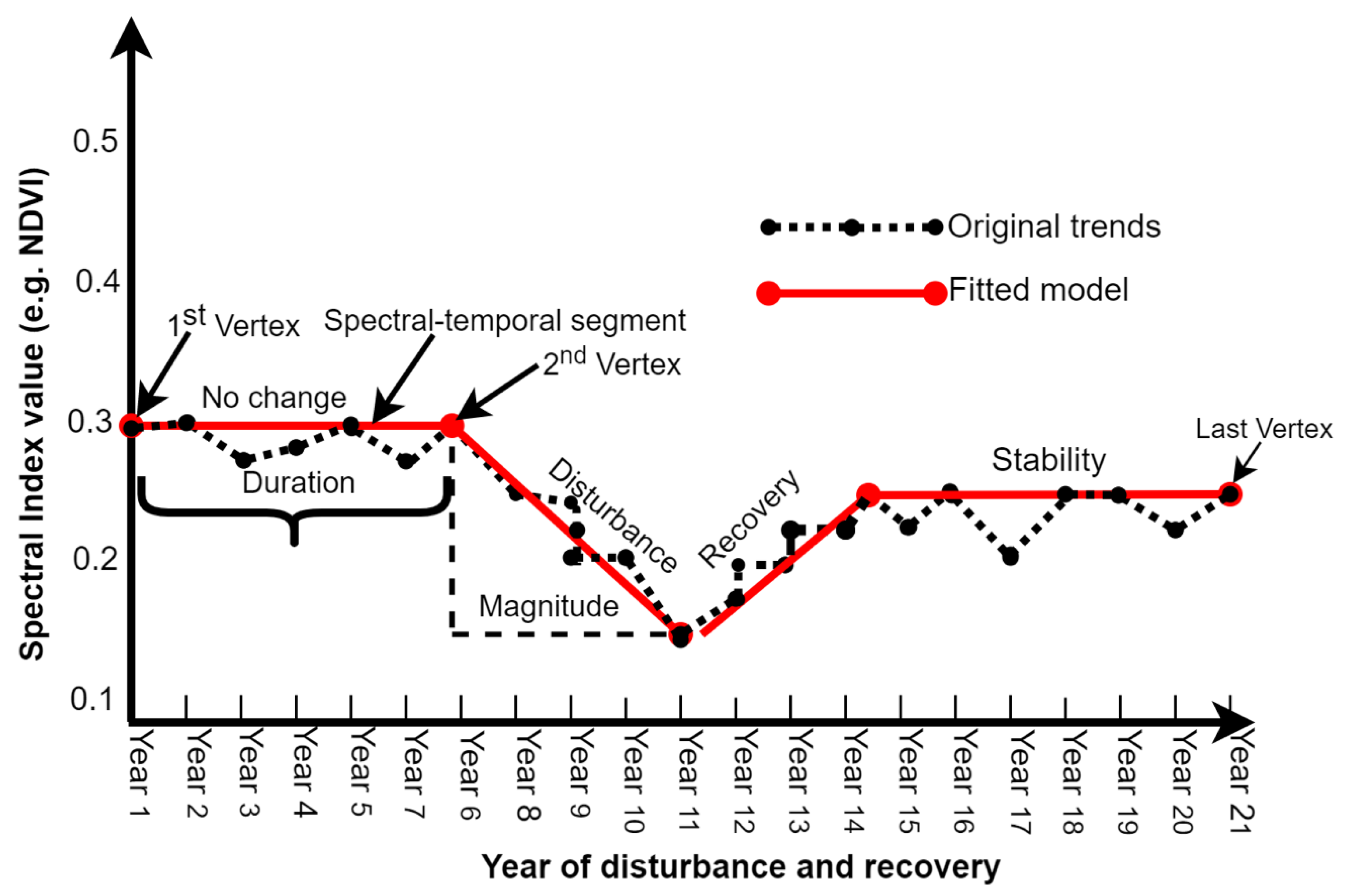
LandTrendr involving the spectral-temporal segmentation of Landsat time series and the complex statistical analysis allowing the extraction of spatial patterns of land cover change magnitude, change duration, and year of change [44].

All time-series change detection algorithms are not producing similar results, even if using the same inputs data [45]. Some algorithms are hard to implement and more demanding in terms of computation requirements. Therefore, users should be cautious about the choice, and the selection should be based on the application domain, supporting computational platform and study objective. The common characteristics for all times series for land change are still a large number of missing data [46] but each of them presents the pros and the cons. For instance, TimeSat was found robust across the large number of its applications, and its flexibility to allow seasonal trend analysis [17]. However, TimeSat-based analysis could be affected by bias emanating from inter-annual variations and fluctuation of seasonal parameters. Despite its robustness in depicting vegetation change processes, particularly forest, VCT is uniquely designed for limited applications.

The performance of EO time series algorithms heavily depends on their accommodating computational platform and parameters to be taken into account. Traditional standalone architecture and personal computers could not efficiently handle advanced EO big data processing tasks [20]. Hopefully, the technology advance enhanced the computation performance through server-client application platforms or through the move to cloud computing. The cloud-based processing platforms allow users the possibility to interact with EO data without investigation in backend computing and data management infrastructures [47] and it is the case for LandTrendr-GEE architecture. While considering the standpoint of ease of use and the development maturity, GEE was identified as one of the best options for big EO data management and analysis [48]. Recently, the implementation of the LandTrendtr algorithm in the GEE platform opened the opportunities for online collection of all available Landsat data and processing them in a cloud-based environment with a user-friendly application programming interface (API) [44].

2. LandTrendr-Google Earth Engine for Analysis of Land Cover Change Trajectories

GEE is a cloud-based geospatial processing platform, offering a large set of user-friendly API for analyzing freely available satellite images, producing statistics and maps, and graphical representation of investigated phenomena through parallel computing [49]. It is mainly composed of two components working in sync with each other, namely Google Earth Engine Playground (EEP) and Google Engine Explorer (EE) [49,50]. On the other hand, LandTrendr is a set of trajectories and spectral-temporal segmentation algorithm that are useful for annual land disturbance and recovery detection taking into account the intensity of the land cover disturbance known as the magnitude of change, the duration of the event expressed in the number of years, and the year when the land disturbance or recovery occurs [35]. The detection is carried out based on collection of Landsat time-series. The algorithm applies the normalization and medoid image stacks and selection process, which makes the spectral space relatively consistent across all Landsat sensors [35]. The medoid selection process consists of comparing and aligning pixels’ values in all visible and infrared red bands of all Landsat sensors to median spectral values in all annual collected images. Values resulting from any spectral transformation can be used for all images irrespective of Landsat sensors [35,44]. LandTrendr was first developed in Interactive Data Language (IDL) software in 2010 [35] and then implemented in the GEE platform in 2018 [44]. It fits the spectral-temporal trajectory to each image pixel in an annual time series and traces the historical evolution of the same pixel in image time series. By referring to one band/index, these trajectories can be used to identify a specific event of land cover change at a pixel level in space and time dimensions. The algorithm provides information on the year of detection, the duration, and the magnitude of each detected change event (see Figure 1).

The LandTrendr algorithm was initially tested in forest disturbance and recovery detection in the Pacific Northwest of the United States of America (U.S.A), western Oregon, and Washington by Kennedy et al. [35]. The findings of their study confirmed that the model outperformed the bi-temporal change detection previously carried out by [51] in tracking forest disturbance and detecting other trends related to forest phenology and regrowth in the same study area. A growing number of studies have subsequently proven the effectiveness of LandTrendr algorithms in investigating the patterns of forest disturbance and recovery (e.g., [52,53]). Furthermore, trends in mining-induced land cover change based on LandTrendr-GEE were successfully tracked respectively in Richards Bay Minerals Site, South Africa [54], and in central east Queensland, Australia [55]. The combination of LandTrendr-based indices and Landsat time-series data allowed analysis of cropland conversion patterns in a 10-year time span around Dongting Lake, China [56], and the detection of impervious surfaces in two urban areas of Jiangsu Province, China, including Nanjing [57] and Xinbei District [58]. LandTrendr-GEE’s application in analyzing urban land cover dynamics and change trajectories is very scanty, thus this needs to be tested. Particularly, the LandTrendr-GEE framework would potentially open the opportunities for urban land cover change analysis in Sub-Saharan Africa (SSA), as the very high-resolution satellite images are expensive and less affordable by local urban planning institutions. Additionally, it is hard to acquire continuously and annually fit-for-purpose optical images for regular monitoring of land cover dynamics, given that atmospheric attenuations sometimes affect the quality of data acquired from optical sensors.

Various approaches are used for urbanization analysis, such as change analysis of spatial temporal variation of land surface biophysical properties using time series indices derived from multispectral satellite data (e.g., [59,60]). These indices include, but are not limited to, the normalized difference vegetation index (NDVI), normalized difference moisture index (NDMI), normalized difference built-up index (NDBI), index-based built-up index (IBI), urban index (UI), enhanced built-up, and bareness index (EBBI), etc. The synergistic use of Landsat time series and the LandTrendr-GEE framework is an added value to the previous urbanization research effort. This framework allows long-term and continuous annual monitoring of land cover change disturbance and recovery analysis. It is also equipped with a fitting model for noise-induced spikes reduction, while detecting interannual land change events [44]. LandTrendr-GEE-based indices/bands are easily portrayed and manipulated in a user-friendly interface with rich information on the magnitude, duration, and year of event change detection. Further statistics on land cover change disturbance and recovery can be extracted, and a fitting model narrating the global trend of landscape change trajectory is visualized. In this research, a framework for analyzing urban land cover change dynamics based on Landsat time series and LandTrendr-GEE is proposed. The study aimed at integrating the baseline land cover change with bands and indices extracted using the LandTrendr algorithm for reconstructing progressive dense annual land cover maps within the considered period. The baseline two land cover maps were generated at the beginning and at the end of the proposed time interval, which is 1987 and 2019, respectively. The proposed framework is believed to be cost-effective and useful for continuous monitoring of complex urban land cover dynamics, especially in environments with EO data affordability issues, and in data-sparse regions. Indeed, LandTrendr-derived data have worldwide coverage and are freely available. Furthermore, the integration of LandTrendr in GEE was judged as a high-performing platform based on open-access software and cloud computing [44,48].

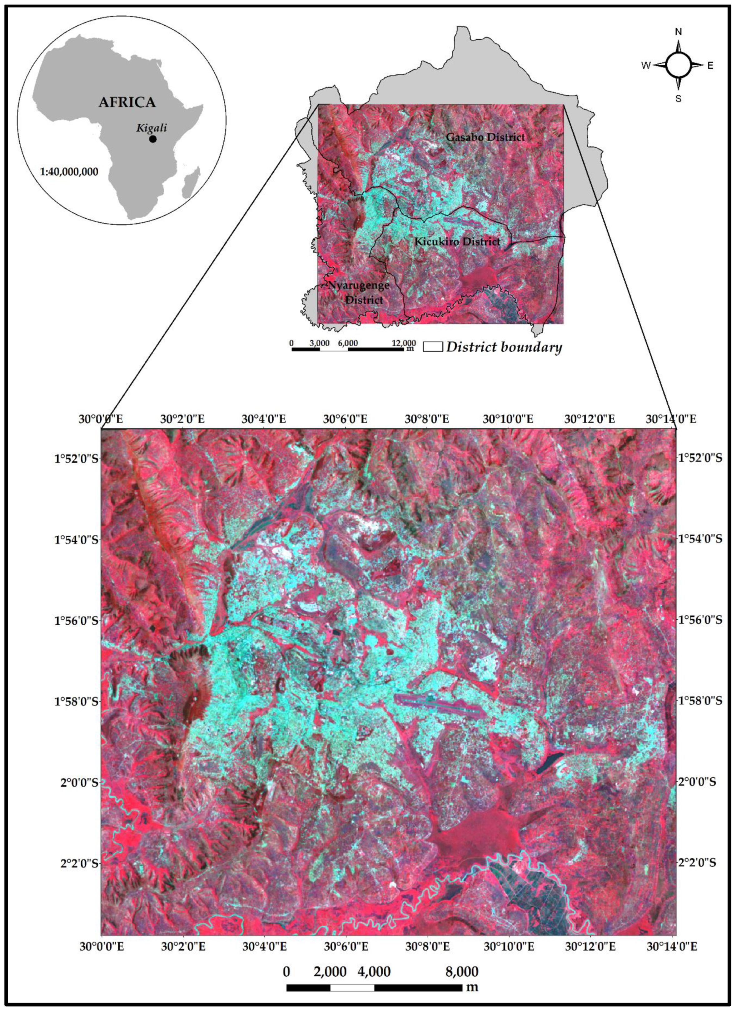
3. Study Area and Data Description

Kigali is the largest and the capital city of Rwanda, a country located in East Africa (see Figure 2). The city, designated initially as Germany’s colonial administrative outpost in 1907, expanded across a small neighborhood plateau around Nyarugenge hill with an estimated 357 inhabitants [61]. The last administrative restructuring took place in 2006 and led Kigali to be a metropolitan area covering 730km², partitioned in three districts including Nyarugenge, Gasabo, and Kicukiro [62]. The 2012 Population and Housing Census illustrated that the Kigali metropolitan area accommodates 1.135 million inhabitants, with a 4.1% annual urban growth rate [63]. Kigali is remains the most important hub of Rwanda’s secondary and tertiary activities, and the main port of entry. According to the 2013 land use [64], around 60.5% of the total city administrative area is dominated by rural agrarian land and marshlands (19.4%). Urbanized area occupies approximately 17%, with informal settlements estimated at 79% of the total built-up areas [65]. Since the implementation of the 2013 Master Plan, which is a long planning process dated back in 2007, urban redevelopment is taking place in the core urban zone through built-up area renovation, the construction of high-rise buildings, road network densification, and parking area modernization. Land conversion, rapid urban expansion in urban fringe neighborhoods, and conurbation translated by satellite towns in the proximity of Kigali administrative boundaries mainly along the national road axes are the observed land change trends. Despite the urban policy and settlement regulations in place, accelerated urbanization observed in Kigali has led to the uncontrolled growth of informal settlements and environmental degradation [66]. Tangible statistics on land use change processes and trajectories are still lacking. Quantification of the change in vegetation proxy and land-use change trajectories in Kigali would contribute to informed decision making about sustainable urban dynamics and land use management. The testing area covered in the present study occupies an area of approximately 609.57km²_. It mainly covers Kigali’s core built-up area and the surrounding urban fringe zones as portrayed in Figure 2.

The Landsat surface reflectance cloud masked composite collections were used for generating the two baseline land cover maps, respectively, the 1987 and 2019 classifications. The collections were accessed, pre-processed from GEE, and exported for further processing by constraining the area of interest in the study area-bounding box. The two composite collections were acquired by filtering the dates corresponding to the image with good quality. Landsat surface reflectance data are atmospherically corrected using the Landsat Ecosystem Disturbance Adaptive Processing System (LEDAPS), and they include a cloud, shadow, water, and snow mask produced using CFMASK, as well as a per-pixel saturation mask as specified in the Earth Engine data catalog (https://developers.google.com/earth-engine/datasets/catalog/LANDSAT_LC08_C01_T1_SR). The first Landsat 5 Thematic Mapper composite (LANDSAT/LT05/C01/T1_SR Path: 172; Row: 061) was constrained between 1 February and 31 December 1987. The 2019 image was acquired using the Landsat 8 Operation Landsat Imager (L8-OLI) sensor with LANDSAT/LC08/C01/T1_SR identification code. It is an annual cloud-masked composite collected by constraining the acquisition between 1 January and 31 December 2019. The Digital Terrain Model (DTM) and slope derived from the DTM were also data sources combined with multispectral bands for land cover classification. The DTM used in this study was produced by the Shuttle Radar Topographic Mission (SRTM) with a resolution of 1 arc-second global product (around a 30-m spatial resolution). More DTM specifications can be retrieved from https://www2.jpl.nasa.gov/srtm/. Annual image collections from L5-TM, Landsat 7 Enhanced Thematic Mapper Plus (L7-ETM+), and L8-OLI from 1987 to 2019 were used for LandTrendr spectral-temporal segmentation and for generating GEE-LandTrendr-based indices. High-resolution Google Earth images were employed for collecting and labeling the validation samples.

4. Methods

In this section, an overview of the methods used in this study is presented and discussed, including the functional architecture of the LandTrendr-GEE framework and various processing tasks.

4.1. Image Pre-Processing

The two Landsat images that served as baseline classification were first co-registered using automatic registration performed in ENVI 5.3 software. L8-OLI was considered as a base image for co-registering the 1987 L5-TM. A cross-correlation matching method and 0.2 minimum matching score were proposed for automatic tie points generation. The image transformation was set as a geometric model, whereas the first-order polynomial transform (RST) was chosen as the transformation model. In total, 100 tie points were proposed, and the ones with more than XY pixels’ reprojection errors were eliminated until we retained 24 high accurate points with a root mean square error (RMSE) > = 0.8. Prior to land cover classification, the Gray Level co-Occurrence Matrix (GLCM) proposed by [67] was computed and stacked with Landsat bands. GLCM is a texture measurement based on second-order statistics for image texture analysis. It quantitatively describes the probability of relationships between the brightness values of neighboring pixels at a distance and orientation invariant within the image [67]. The output consists of a single two-dimension raster layer containing derived measurements for all pixels and may be input into further analysis [68]. In the present study, the use of GLCM as input in the feature space was motivated by the fact that previous studies (e.g., [69,70]) illustrated the utility of GLCM texture features in improving land cover class separability. Derived GLCM texture features concerned the mean, variance, contrast, and standard deviation computed from red, green, and near-infrared bands of both 1987 L5-TM and 2019 L8-OLI. The GLCM was calculated in the four main orientations (i.e., 0, 45, 90, and 135) with a one-pixel shift and 11 × 11 kernel size. The experimental results in the previous studies found that the best urban classification results would be achieved with a kernel size ranging from 5 × 5 to 13 × 13 [71,72] and 11 × 11 kernel was found to be optimal for the best urban land cover classification [73,74].

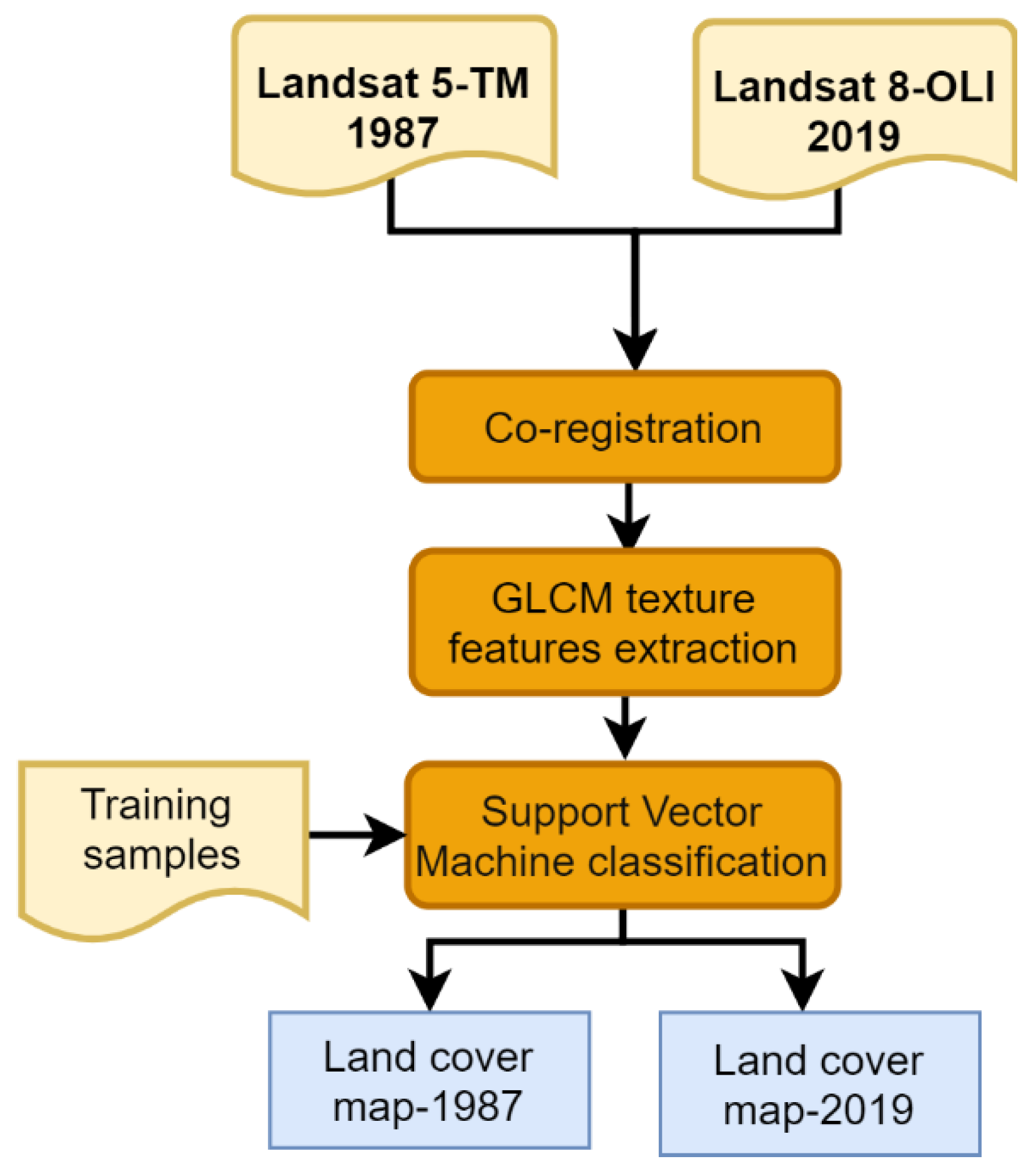
4.2. Baseline Land Cover Classification

Five land cover classes were proposed in the land classification scheme, as specified in

Table 1. Proposed land cover classification scheme and the corresponding description.

Land Cover Type	Description
Urban	Areas composed of high and low-density built-up areas, sealed surfaces, including paved road networks, airport, and parking lots
Open land	Areas occupied by cultivated lands, glass land, urban green spaces, and bare land
Forest	Areas covered by mature vegetation of height > 5 m with ≥ 60 % ground surface covered by trees and canopy with evergreen foliage. This class includes native montane forests, secondary (derived) forests, and forest plantations
Wetland	Low land zone characterized either by permanent flooded zones with vegetated cover or seasonally flooded low land occupied by cropland and surrounded by highlands with a steep and moderate slope
Water	Permanent water bodies such as lakes, fish ponds, water table in irrigated land, and water channels mainly composed of permanent watercourses

. Before the GEE processing chain, a pixel-based support vector machine (SVM) classifier was applied to generate baseline and keyframe land cover maps for the predefined starting and ending time periods. SVM is a non-parametric supervised classifier based on statistical learning theory [75], which has outperforming properties, including effectiveness in segregating multimodal classes [76], good generalization ability, and efficiency in handling data in high-dimensional feature spaces [77]. Previous studies (e.g., [78,79,80]) illustrated the SVM as one of the top best-performing classifiers for satellite image land cover classification. Figure 3 illustrates the step-by-step processing chain followed for generating the 1987 and 2019 land cover keyframe classification.

The training samples were determined by referring to the random sampling design. Five land cover classes were proposed in the classification scheme, including the built-up area (BUA) corresponding to settlements and sealed/impervious surface, open land mainly composed of either agricultural areas or permissive uncovered land, forest, wetlands, and water. In total, 572 samples were proposed for the 1987 classification, while 647 were selected for the 2019 image classification. The computed GLCM layers, together with DTM and slope, were stacked with classic Landsat bands for the training of the SVM classifier. The SVM Radian Basic Function kernel (RBF) was chosen for generating the classified maps. Post-processing operations, such as class aggregation, were performed for smoothing the classification.

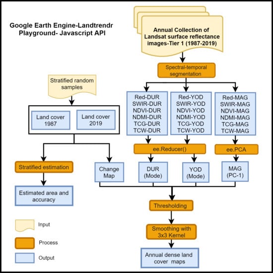
4.3. Processing Chain in GEE

The processing steps performed in GEE include the spectral-temporal segmentation and LandTrendr-based analysis, predicting progressive land cover maps and associated statistics, and accuracy assessments using the GEE-based area estimation and accuracy Assessment (Area²) application.

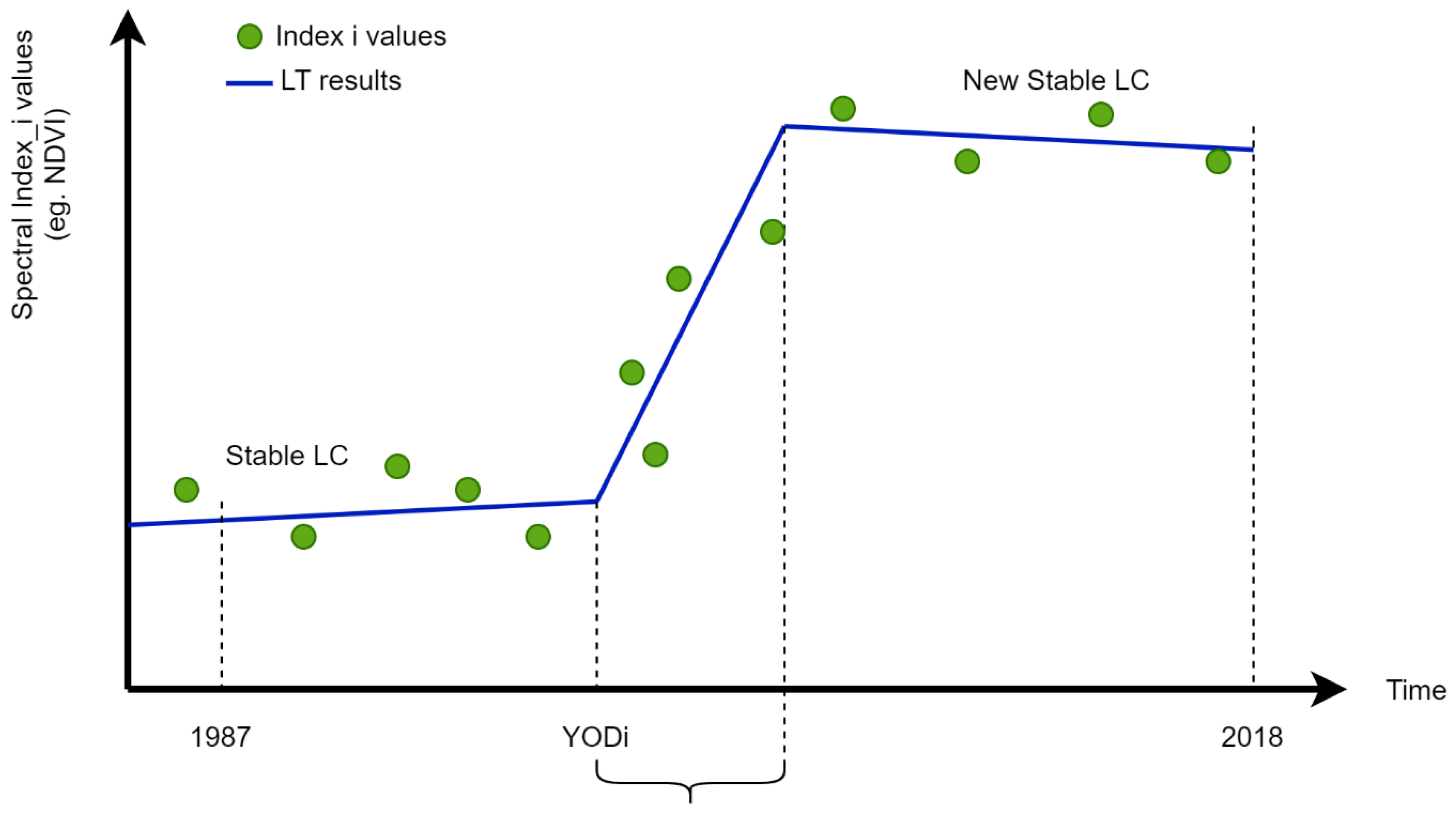
4.4. Spectral-Temporal Segmentation and Analysis

GEE was used to analyze the stacks of Landsat images using the LandTrendr (LT) algorithm. Spectral-temporal metrics were constructed from 1987 to 2019 based on images acquired from L5-TM, L7-ETM+, and L8-OLI. Landsat annual collections were constrained to the date range from 1 September to 30 June of the following year. This time span corresponds to the two main rainy seasons, and the short-term dry season in the study area. The optimal land cover representation during the proposed time range could be effectively inventoried. To trace the land cover changes, we proposed the use of a combination of six indices/bands, including red (R) and shortwave infrared (SWIR) bands, NDVI, NDMI, Tasseled Cap Greenness (TCG), and Tasseled Cap Wetness (TCW). The selection of these bands and indices for spectral-temporal segmentation was first based on visual inspection of the LandTrendr results.

The best candidate indices/bands were those judged that were able to highlight more changing patterns and those that were believed to capture valuable information related to the land surface properties in the study area. The NDVI was expressed as a normalized transformed ratio between R and near-infrared (NIR) bands (NDVI = (NIR-RED)/(NIR+RED)) [81], which was selected because it is the most widely used index for land cover assessment [82,83]. NDVI was also previously proved worthwhile in greenness proxy monitoring in urban and peri-urban environments [84,85]. The NDMI index is a normalized ratio between NIR and SWIR (NDMI = (NIR-SWIR)/(NIR+SWIR), and it was found to be useful for tracking changes in plant biomass [86]. We assumed that cropland conversion to impervious surfaces is associated with a decrease in the NDMI value. The two features of tasseled cap transformation (i.e., TCG and TCW) were found to be valuable for providing mechanisms for spectral data dimensionality reduction with minimal information loss [87,88], and they were previously applied for enhancing urban land cover change analysis (e.g., [12,89,90]). We adopted the tasseled cap transformation coefficients defined for reflectance data, as proposed by [91]. These coefficients were successfully adopted in previous LandTrendr-related studies (e.g., [35,52]) involving the use of annual collection of stacked Landsat time series. Orthogonal cap transformation for the wetness and greenness indices (TCG and TCW) is respectively expressed by Equations (1) and (2):

$$\mathrm{TCG}=-0.1602*\mathrm{Blue}-0.2819*\mathrm{Green}-0.4934*\mathrm{Red}+0.7940*\mathrm{NIR}-0.00002*\mathrm{SWIR}\_1-0.1446*\mathrm{SWIR}\_2$$

(1)

$$\mathrm{TCW}=0.0315*\mathrm{Blue}+0.2021*\mathrm{Green}+0.3102*\mathrm{Red}+0.1594*\mathrm{NIR}-0.6806*\mathrm{SWIR}\_1-0.6109*\mathrm{SWIR}\_2$$

(2)

4.5. Progressive Land Cover Reconstruction

The LT algorithm is designed to analyze a single index/band, while integrating many logical decision steps and statistical tests to detect land cover disturbance and recovery [52]. In the present study, we proposed a new methodology to integrate multiple indices and to use two available land cover maps as keyframes for labeling the LT-detected changes that occurred during the analyzed period. Figure 4 portrays the proposed workflow for LT-GEE for reconstructing land cover change trajectories and applying the Area² methodology to estimate the area and accuracy assessment.

For reconstructing yearly land cover maps, we stacked all the LT results generated using a single index/band to obtain a complete and more reliable detection of the changes that occurred during the period. In particular, we adopted different strategies to combine the three outputs of LT: The year of change detection (YOD), the change detection duration (DUR), and the change detection magnitude (MAG).

For the MAG outputs, we stacked together the four indices and two bands, and we applied a principal component analysis (PCA). Considering that the LT MAG results have a great amount of no-data values (see Figure 5) and that these values are not in the same location for the different stacked layers, we adopted a median filling procedure to interpolate the values of the no-data pixels using the values of the surrounding pixels. The implementation of the PCA algorithm with a median filling strategy for missing values has been implemented in the GEE platform. We selected the first PCA band (PC-1) as the most informative band that is able to combine the common pattern detected in most of the indices and this procedure substantially improves the reliability and the completeness of the LT magnitude results.

The LT YOD and the LT DUR results portray data range values illustrating the absolute year of change disturbance, and the number of year(s) the change or the stability of the disturbance event last. For deducting LT YOD and the LT DUR results based on stacked four indices and two bands, we adopted a strategy different from the one used for deducting the magnitude of change (MAG) to keep the original data range and measurement unit. We realized that applying PCA to the data range would result in transformed values. While it was important to keep the measurement unit expressed in years (for the case of YOD and DUR) to be able to retrieve the correct year of change, we adopted the GEE based "reduce by mode" function for separately deducting the LT YOD and the LT DUR based on LT based on stacked four indices and two bands (see Figure 4).

For each pixel in the LT stacked results, we observed and computed YOD and DUR values as illustrated in Figure 6. We further detected the land cover change that starts at the YOD and, we investigated the time when the change trend stabilized after a period of perturbation (DUR). Starting from these two values, we could estimate the YOC (year of change) and the time the corresponding pixel can be labeled as the new land cover class. This simplification of the LT results was required to label the pixel in a land cover class and to obtain yearly land cover maps. We further used a weighted mean procedure to estimate the corresponding YOC (see the formula for the weighted YOC formula in Equation (3)), in which we assumed that the YOC is the central value of the disturbance period. We also weighted the sharp detection (short DUR), which was considered useful for observing the change in a very short period:

$$\begin{array}{l}YOC=\frac{{\displaystyle \sum _{i=1}^n\frac{1}{2}}\left((YO{D}_i{+DUR}_i)\right)\frac{1}{DU{R}_i}}{{\displaystyle \sum _{i=1}^n\frac{1}{DU{R}_i}}}\end{array}$$

(3)

By combining the MAG-PC1 and YOC layers in each year, it was possible to reconstruct the land cover trajectories over the period 1987-2019 and produce the annual land cover maps. We used a threshold value to consider only the changes with a significant MAG and that were detected before the considered year (YOC < target land cover map year). The followed steps in GEE can be accessed via https://code.earthengine.google.com/cd2666b30174d7e728fef70eac6be7a4?accept_repo=users%2Femaprlab%2Fpublic.

4.6. Results Validation and Quality Assessment

Area estimation and accuracy assessment (Area²), which is a GEE application that provides support for sampling and estimation in a design-based inference framework [92], was used for quality assessment. The baseline classification maps for reconstructing progressive land cover maps were first imported in GEE Asset Manager and then displayed in GEE code editor. By referring to the Area² application, stratified random sampling was adopted for the proportional area estimate and accuracy among strata. According to the Area² approach, the sample size is determined using Equation (4):

$$\begin{array}{l}n={\left(\frac{{\displaystyle {\sum }_h{W}_{h}S{D}_h}}{SE\left(\widehat{y}\right)}\right)}^2\end{array}$$

(4)

where

• n is the number of samples;
• W_h are the stratum weight corresponding to the weight of each of the proposed land cover classed;
• SD_h are the stratum area standard deviations;
• $\mathrm{SE}\left(\widehat{y}\right)$ is the target standard error of the stratum area estimate

By adapting Equation (4), 1481 random samples were proposed for 1987 and 1500 samples in 2019 for area estimate and accuracy assessment. The areal weight for each stratum (i.e., each of our adopted land cover classes) was determined and used for allocating the number of samples. The more the stratum weight is significant, the more the number of samples were allocated [92]. High-resolution Google Earth imagery and background Landsat images were used for collecting and labeling validation samples. A stratified estimator was adopted for computing the strata proportion area estimate, standard error quantification, and accuracy assessment. The 95% confidence interval (CI) with a 0.005 margin error was adopted for accuracy assessment. The stratified estimator is expressed as the sum of the means of the simple random samples within strata weighted by stratum weights calculated as relative proportions of the population within strata [92,93]. The progressive maps were also assessed using the same area² procedures. The 2019 baseline validation samples were used across all five-year-interval reconstructed maps using the proposed elimination and gap-filling approach. The latter consisted of first extracting the binary change mask (changed/unchanged) for each considered YOC based on 2019 and the considered YOC land cover. Validation points falling inside the changed zones in the mask were then eliminated and new samples were collected for compensating for the eliminated ones. This strategy was found to be useful for rationalizing and saving time for collecting validation samples, but an increase of additional samples is paramount. As proposed by [92], the producer’ and user’s accuracies, and overall accuracy are expressed as follows:

$${Û}_i=\frac{{\widehat{p}}_{ii}}{{\widehat{p}}_{i.}}$$

(5)

$${\widehat{P}}_j=\frac{{\widehat{p}}_{jj}}{{\widehat{p}}_{.j}}$$

(6)

$$\widehat{O}={\displaystyle \sum _{j=1}^q{\widehat{p}}_{jj.}}$$

(7)

where

• i: Mapped category represented in row
• j: Reference category represented in column
• q: number of considered categories
• ${Û}_i$: User’s Accuracy in class i
• ${\widehat{P}}_j$: Producer Accuracy in category j
• $\widehat{O}$: Overall Accuracy

5. Results

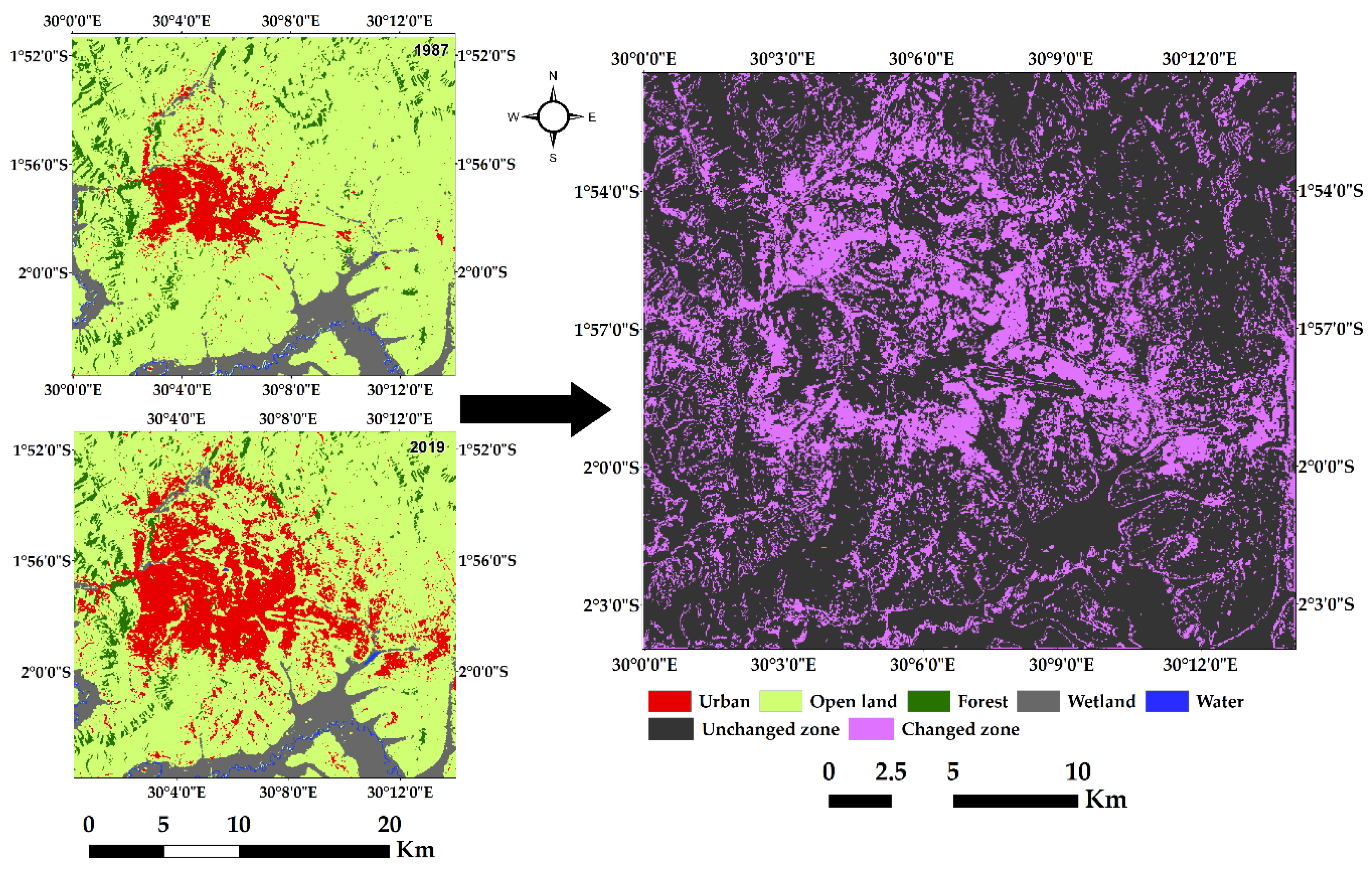
5.1. Baseline Urban Land Cover Classification

The baseline urban land cover maps were generated with an overall 92%±1.6% classification accuracy in 1987 and 94.2%±1.6% in 2019 with a 95% confidence interval. A significant change is remarkable in Kigali in the last 32 years, from 1987 to 2019.

Table 2. Estimated area and accuracies with a 95% confidence interval for the baseline land cover classification.

1987
Land Cover Classes	Urban	Open Land	Forest	Wetland	Water
Class area proportion	0.078	0.736	0.071	0.11	0.005
Standard error	0.005	0.008	0.004	0.005	0
Area (ha)	4782.99	44884.99	4321.57	6688.63	279.45
95% CI (ha)	642.49	957.88	491.72	547.26	18.85
User’s accuracy	0.94 ± 0.02	0.94 ± 0.02	0.90 ± 0.036	0.97 ± 0.037	0.93 ± 0.062
Producer’s accuracy	0.73 ± 0.13	0.98 ± 0.021	0.84 ± 0.114	0.88 ± 0.082	1 ± 0.067
Overall Accuracy ( ± 95% CI) 0.942 ± 0.016
2019
Class area proportion	0.234	0.587	0.067	0.106		0.006
Standard error	0.006	0.008	0.003	0.004		0
Area (ha)	14432.05	36224.59	4142.24	6518.98		389.95
95% CI (ha)	760.10	977.79	406.24	506.06		12.53
User’s accuracy	0.94 ± 0.022	0.92 ± 0.022	0.95 ± 0.026	0.89 ± 0.058		0.98 ± 0.032
Producer’s accuracy	0.85 ± 0.53	0.95 ± 0.027	0.85 ± 0.098	0.93 ± 0.078		1 ± 0.032
Overall Accuracy ( ± 95% CI) 0.92 ± 0.016

CI: Confidence Interval

illustrates the land cover classification statistics in two considered extreme dates, while Figure 7 portrays the binary change detection maps where both unchanged and changed zones are visualized.

Land cover dynamics between 1987 and 2019 illustrate that 27% of the study area corresponding to 16,750 ha was subjected to change. At the class level, the results illustrate that compared to the 1987 situation, urban area increased by 198.4%, whereas open land was reduced by 16.7%. Open land was mainly converted to urban class. Even if the water class was slightly changed, dense annual land cover maps revealed the emergence of small water patches in the central part and in the southeast of the study area. Compared to previously stated classes, the area occupied by wetland was found more or less stable and the forest class was less affected by the change. This does not mean forest and wetland were not altered in Kigali City administrative entities, because the main changes of the two last classes were found in areas beyond the bounding box of the present study area.

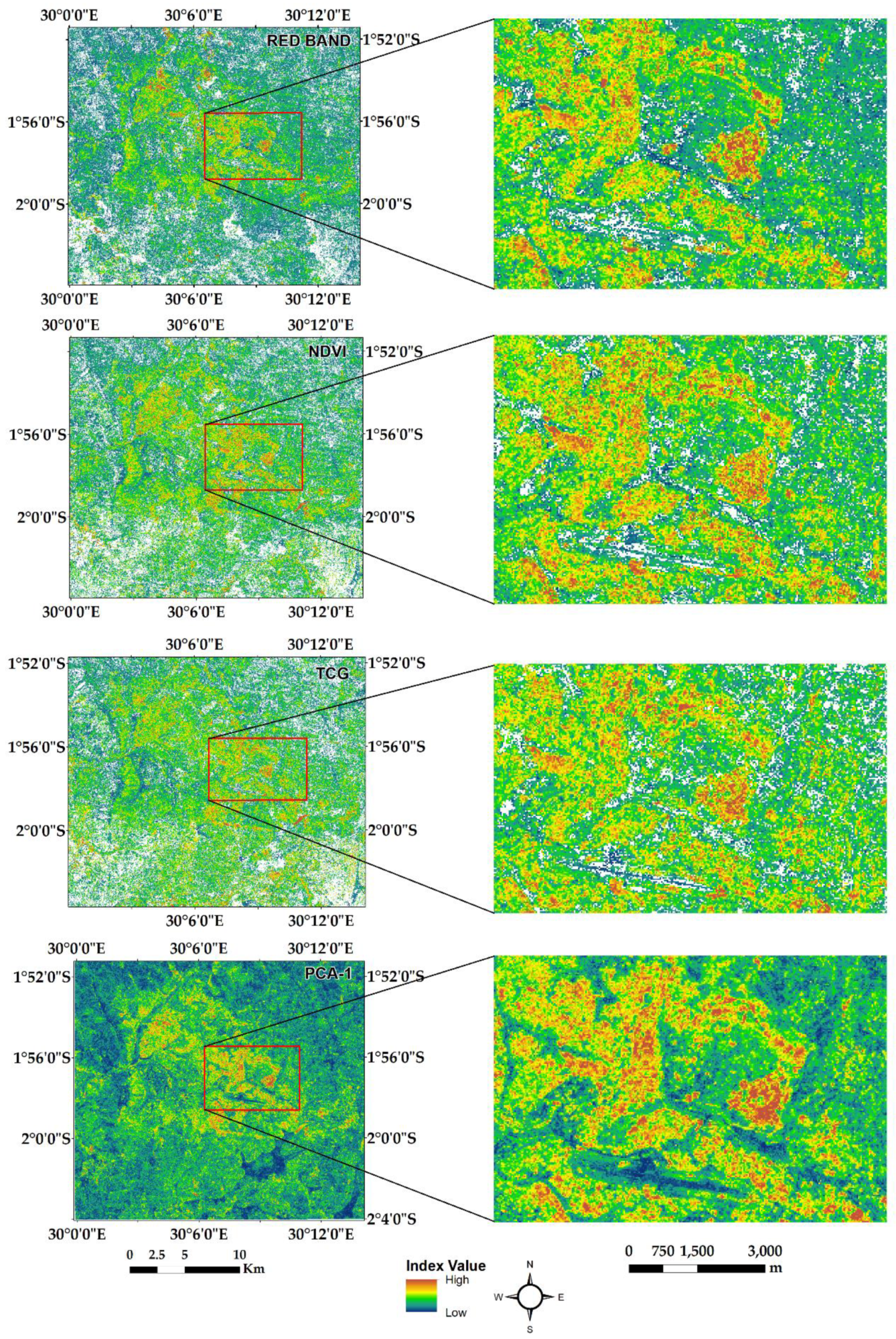
5.2. LT-GEE Parameter Configurations and Spectral Indices’ Characterization

LT requires several parameters from which spectral-temporal segmentation and land cover trends analysis could be feasible. According to Kenned et al. [44], eight control parameters and annual Landsat images collection are mandatory for deriving either an index or a single band telling the pixel’s story background evolution. In the light of achieving the best results, different combination values of algorithm parameters were tested, and the judged optimal values are illustrated in

Table 3. GEE-LT optimal segmentation parameters.

Parameters	Data Type	Proposed Value
Max segments	Integer	8
Spike threshold	Float	0.9
Vertex count overshoot	Integer	3
Prevent one-year recovery	Boolean	True
Recovery threshold	Float	0.25
p-value threshold	Float	0.05
Best model proportion	Float	0.75
Min observations needed	Integer	6
Time series collection	L5-TM, L7-ETM+, and L8-OLI

.

For the purpose of the present study, we used the standard configuration parameters as specified by the algorithm pioneers [35]. We simply adapted the number of maximum segments as the pioneer recommended that this could be adopted, provided that it is helpful in detecting the disturbance and recovery of land cover dynamics in the considered study area. We found that an 8-value set for maximum segments was helpful is detecting land cover disturbance in the study area. Other parameters were kept as they were originally defined. The value derived from specific indices, such as NDVI and TCG, illustrated that a short change duration (less than 5 years) is always associated with a high change magnitude since circa 2008. In general, it took the completely covered period corresponding to 32 years to see the change in a big part of the study area. This translates that the land change processes were gradual, especially in old urban areas and in crop-dominated land. However, newly urbanized and converted areas are characterized by a high change magnitude and abrupt change duration.

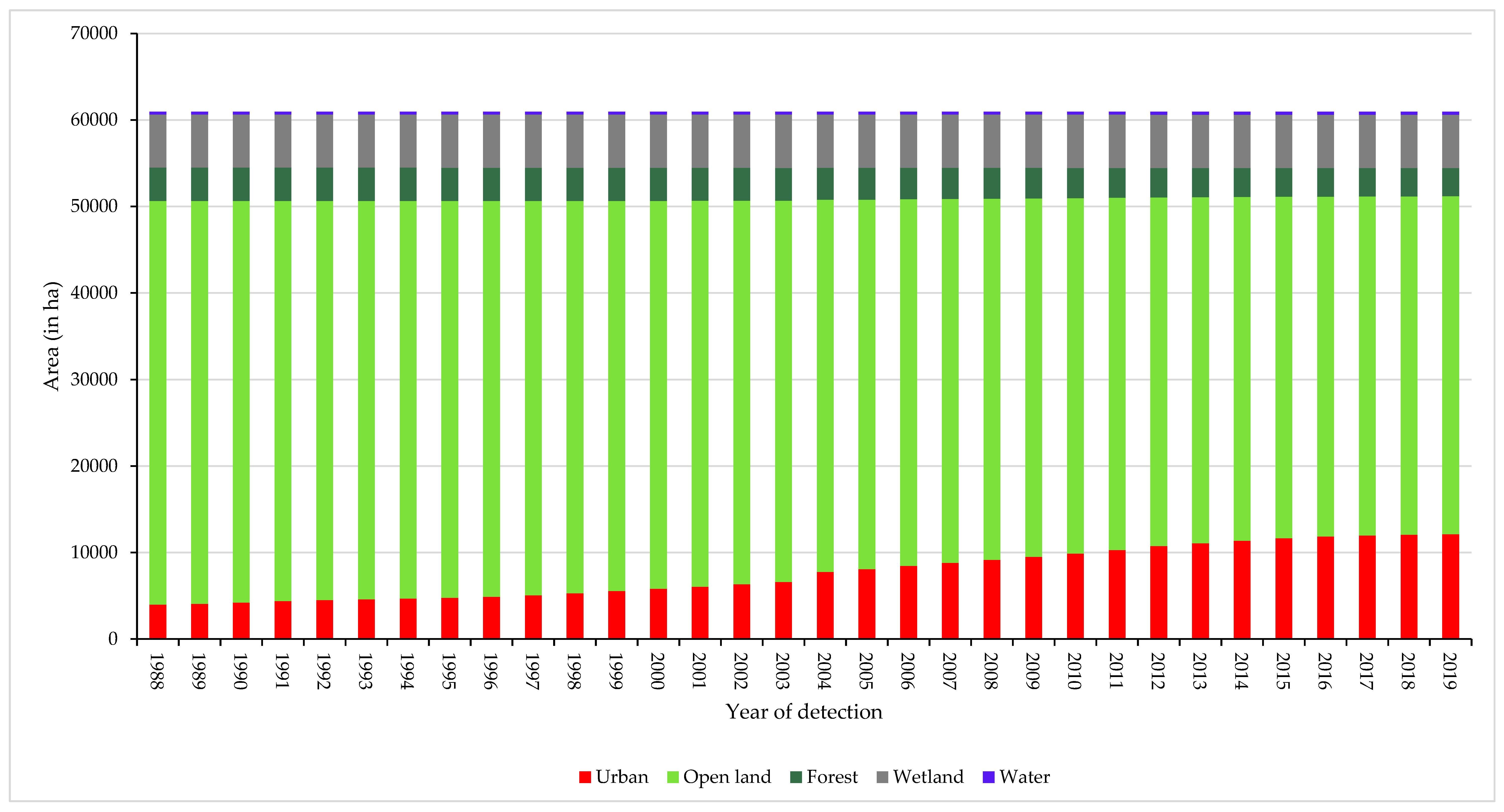
5.3. Progressive Land Cover Reconstruction Based on the LT-GEE Framework

The synergy between the baseline change maps and LT-GEE-derived indices/bands allowed reconstruction of the annual land cover change maps from 1988 to 2019. Since 1988, tremendous land cover conversion, mainly from cropland to impervious areas, and urban expansion were witnessed across the Kigali city landscape. The study results illustrated extensive urban growth between 1987 and 2019, with a 226.4% growth rate. The five-year term analysis from 1990 to 2015 illustrated that impervious surfaces increased from 4233.5 to 11648.29 hectares (see

Table 4. Land cover change from 1990 to 2015 based on derived from combined LandTrendr indices and classified Landsat baseline frames.

	Area (in ha)
	1990	1995	2000	2005	2010	2015
Urban	4233.51	4779.62	5813.57	8099.01	9892.77	11648.29
Open land	46397.33	45851.02	44832.81	42696.50	41071.18	39473.76
Forest	3869.73	3856.78	3821.85	3677.54	3493.34	3328.13
Wetland	6142.25	6153.15	6167.05	6158.47	6165.54	6164.07
Water	307.99	310.23	315.51	319.29	327.98	336.55

), with 3.7% average annual urban growth rate.

Land cover change trajectories portray a conversion to urban class mainly following the eastern, southern, and northern directions. In contrast, the western areas were less converted as illustrated in the land cover maps represented in Figure 8.

The interannual change analysis revealed that gradual change to urban structures was observed from 1988 to 1991, with an average annual urban growth rate of around 3.4%. During that time span, the built-up area extended from 3976 to 4405 hectares. The period from 1991 to 1995 was characterized by a decreasing urban growth, with an annual average rate ranging between 1.8% and 2%. The slow urban progress during this period could be explained by socio-economic and political instability and economic recession in Rwanda, which characterized the abovementioned period. Indeed, the 1991-1995 period coincided with the five-year war and armored conflict that culminated with the 1994 genocide against Tutsi in Rwanda. The post-genocide period was characterized by an urbanization take off. From 2004 onwards, continuous urban expansion was observed, with an increase in annual urban growth averaged to 4%. The post-genocide reconstruction period, especially from 2004, was characterized by servicing new construction sites and built-up area expansion, such as the construction of the Kigali Special Economic Zone, expansion of Kigali International Airport, densification of tarmac roads, and estate development in various zones of the city. This period also coincided with important migration flux to Kigali of the newly repatriated Rwandan refugees who were mainly living in neighboring countries. Since 2014, the continuous and gradual urban growth is observed with an incremental increase (see Figure 9). A probable cause would be linked to the urban policy enforcement translated by new urban planning regulation and construction standards imposed after endorsing the 2013 revised Kigali City Land Use Master Plan [65], and the integration of the city growth perspective in Rwanda Vision 2020 [94]. Endorsed planning standards and regulations are more or less limiting the spread of illegal and deprivation areas. Taking into account the five years of progress of the land cover change interval from 1990 to 2015, the accuracies, class area proportion, and standard error for each land cover class are reported in

Table 5. Estimated error matrix of sample counts with class weight, standard error, producer’ and user’s accuracy, and overall accuracy with a 95% confidence interval. Map categories are presented in rows while reference categories are in columns.

2015
		Reference class
		Ur	OL	For	Wet	WT	Total	Wi	SE	PA	UA	OA
Map class	Ur	238	13	0	1	0	252	0.217	0.0076	0.82 ± 0.069	0.94 ± 0.028	0.92± 0.02
	OL	28	437	4	6	0	475	0.632	0.0095	0.96 ± 0.030	0.92 ± 0.024
	For	0	6	52	0	0	58	0.047	0.0033	0.88 ± 0.140	0.90 ± 0.079
	Wet	0	7	0	65	0	72	0.100	0.0050	0.91 ± 0.097	0.90 ± 0.069
	WT	0	0	0	1	40	41	0.005	0.0001	1 ± 0.049	0.98 ± 0.048
	Total	266	463	56	73	40		1
2010
		Reference class
		Ur	OL	For	Wet	WT	Total	Wi	SE	PA	UA	OA
Map class	Ur	227	11	0	1	0	239	0.205	0.0077	0.81 ± 0.074	0.95 ± 0.028	0.92 ± 0.02
	OL	28	436	4	6	0	474	0.643	0.0096	0.97 ± 0.029	0.92 ± 0.024
	For	0	6	52	0	0	58	0.048	0.0034	0.88 ± 0.140	0.90 ± 0.079
	Wet	0	7	0	65	0	72	0.100	0.0050	0.91 ± 0.098	0.90 ± 0.069
	WT	0	0	0	1	37	38	0.005	0.0001	1 ± 0.053	0.97 ± 0.052
	Total	255	460	56	73	37		1
2005
		Ur	OL	For	Wet	WT	Total	Wi	SE	PA	UA	OA
Map class	Ur	222	7	0	1	0	230	0.199	0.0078	0.79 ± 0.077	0.97 ± 0.024	0.92 ± 0.02
	OL	29	435	4	6	0	474	0.649	0.0097	0.97 ± 0.029	0.92 ± 0.025
	For	0	6	51	0	0	57	0.048	0.0035	0.88 ± 0.142	0.90 ± 0.080
	Wet	0	7	0	65	0	72	0.099	0.0050	0.90 ± 0.099	0.90 ± 0.069
	WT	0	0	0	1	32	33	0.005	0.0001	1 ± 0.061	0.97 ± 0.059
	Total	251	455	55	73	32		1
2000
		Ur	OL	For	Wet	WT	Total	Wi	SE	PA	UA	OA
Map class	Ur	383	3	0	0	0	386	0.104	0.0057	0.81 ± 0.109	0.99 ± 0.009	0.95 ± 0.02
	OL	12	431	4	6	0	453	0.735	0.0086	0.98 ± 0.023	0.95 ± 0.020
	For	0	6	49	0	0	55	0.054	0.0040	0.88 ± 0.146	0.89 ± 0.083
	Wet	0	5	0	65	0	70	0.103	0.0051	0.90 ± 0.097	0.93 ± 0.061
	WT	0	0	0	1	23	24	0.004	0.0002	1 ± 0.085	0.96 ± 0.082
	Total	395	445	53	72	23		1
1995
		Ur	OL	For	Wet	WT	Total	Wi	SE	PA	UA	OA
Map class	Ur	78	3	0	0	0	81	0.072	0.0023	0.98 ± 0.064	0.96 ± 0.041	0.96 ± 0.01
	OL	1	428	5	5	0	439	0.766	0.0071	0.98 ± 0.018	0.98 ± 0.015
	For	0	6	46	0	0	52	0.057	0.0046	0.85 ± 0.159	0.89 ± 0.088
	Wet	0	5	0	65	0	70	0.102	0.0050	0.91 ± 0.096	0.93 ± 0.061
	WT	0	0	0	1	20	21	0.004	0.0002	1 ± 0.098	0.95 ± 0.093
	Total	79	442	51	71	20		1
1990
		Ur	OL	For	Wet	WT	Total	Wi	SE	PA	UA	OA
Map class	Ur	76	3	0	0	0	79	0.069	0.0023	0.97 ± 0.066	0.96 ± 0.042	0.96 ± 0.01
	OL	1	426	5	5	0	437	0.768	0.0072	0.98 ± 0.018	0.98 ± 0.015
	For	0	6	47	0	0	53	0.058	0.0046	0.85 ± 0.157	0.89 ± 0.086
	Wet	0	5	0	64	0	69	0.101	0.0050	0.91 ± 0.097	0.93 ± 0.062
	WT	0	0	0	1	20	21	0.004	0.0002	1 ± 0.098	0.95 ± 0.093
	Total	77	440	52	70	20		1

Ur = Urban; OL = Open land; For = Forest; Wet = Wetland; WT = Water; W_i = Class Weight; SE = Standard Error; PA = Producer’s Accuracy; UA = User’s Accuracy; OA = Overall Accuracy.

.

The overall accuracies in all considered timespans are exceed 92% with a margin error between 1% and 2%. The urban class progressively increased its weights vis-à-vis to others, while open land decreased in weights. In general, the standard error (SE) is less than 0.01, except in the open land class where SE increased to that threshold, respectively, in 2005, 2010, and 2015.

6. Discussion

The present study aimed to design a method for reconstructing annual and dense land cover change dynamics in complex urban environments based on LT and baseline land cover maps. We used Kigali, Rwanda as a case study in the global south nations characterized by a continuous urbanization increase. The case study portrays urban environments with a rapid spread of informal settlements and unregulated constructions in the last three decades since 1987. We adopted the combination of LT-derived indices and bands as a way of deducting reliable intermediate results, such as PCA, applied for filling the gaps observed in the magnitude of land cover change event, and the application of the reduce function for having filled layers representing the duration of land cover change events and the corresponding year of detection. These results were helpful for producing reliable land cover classification and reconstructing annual dense land cover in the study area. The combination of keyframe classifications in two proposed extreme periods, with derived LT indices, allowed continuous annual land cover reconstruction from 1987 to 2019.

6.1. Benefits from LT-GEE in Continuous Land Cover Reconstruction

A cloud computing environment, such as GEE, was found to be worthwhile in data discovery, and in handling multidimensional datasets. LT-GEE allows multifunctional data processing, and the GEE playground offers a user-friendly API and straightforward possibilities for statistics extraction, and interactive data visualization at the intermediate and final processing stages. Furthermore, the GEE platform allows the users to share scripts and assets [48,49], and this capability is paramount for collaborative knowledge generation and experience sharing. The GEE-based area² application was found to be useful in both scrutinizing the quality of the results and predefining the acceptable error margin. It is well known that cloud cover, shadows, and other data gaps, such as the L7 ETM+ scan-line collector failure experienced after May 31, 2003 [95], constrain users to extracting continuous land cover on an annual basis as needed. The GEE-LandTrendr framework was found as an additional solution together with existing gap-filling methods. For characterizing the change in land cover properties, we used six indices. Previous studies (e.g., [53,54,55,56,57]) that involved the use of the LT algorithm in quantifying land cover disturbance had separately relied on evaluating a single index in change detection. Our study illustrated that the combination of several indices in characterizing the land surface properties was deemed useful. Our results concur with the findings by [45], where they emphasized that different indices in time series analysis are useful instead of relying on a single band/index. The GEE-LandTrendr framework was also found to be extendable and customizable. The indices were combined considering the first principle component (PC-1) that was used for computing the change magnitude with filled no-data values. The failure to use PCA and relying on the use of a single LT index would result in the maps having gaps and discontinuous patches that could negatively affect the interannual land cover change trajectories analysis in the study area.

6.2. Methodology Transferability and Limitations

The transferability of land cover classification-related rules is deemed to be more or less consistent when tested in different study areas [96,97]. The GEE-LandTrendr framework can be successfully tested in any site, given the availability of annual Landsat composite imagery. However, the indices used to characterize the landscape under investigation need to be site specific depending on their capability of reflecting the quasi-situation of land surface properties and their spatial coverage. The value of magnitude could be customized for meeting the local situation based on experimental trials. The main bottleneck in using the GEE-LandTrendr framework is still the lack of high-quality image acquisition in a specific area of interest, given the persistence of cloud cover and haze affecting the optimal imagery, such as Landsat. Some indices can reflect the over/underestimated value. The annual land cover reconstruction could be affected by outlier values in stacked indices, and this could affect the spatial-temporal interpolation. Thus, calibration and verification would enhance the production of high-quality land cover maps. In some circumstances, LandTrendr-derived indices are characterized by a large number of no-data values, and deducting their associated value would be incomplete in spatial coverage. This drawback is also found in many methods designed for time series analysis, as reported by [46]. From our experiment, the above challenge could be compensated by stacking many indices and applying the MapReduce function or principal components analysis. The proposed framework for handling gap-fill challenges could be an added value to the existing methods for compensating incompleteness sensitivity while performing EO time series analysis. The performance of one or another LandTrendr index was beyond the scope of the present study. We intend to explore the role and the ranking of each index in different study sites in the future research direction.

7. Conclusions

In this study, a new GEE-LandTrendr cloud-computing framework based on Landsat time series and LT stacked bands and indices for reconstructing annual land cover maps was developed. The resulting dense maps and statistics were found to be worthwhile for better understanding the spatial-temporal land cover change trajectories in Kigali, Rwanda over the past 32 years from 1987 to 2019. Two land cover maps at the start and at the end of the proposed timeframe were first extracted based on Landsat images using a pixel-based SVM classification. A scheme of five land cover classes, including urban, open land, forest, wetland, and water, was selected to understand the urbanization phenomena in the study area. Then, the LandTrenndr-Google Earth Engine platform was used to retrieve the annual collection of Landsat images for tracing the historical evolution of urban land cover change trajectories through the derived LT bands and indices. Control parameters for running the LandTrendr algorithm were set for extracting the duration, the year, and the magnitude for each of the proposed LandTrendr bands/indices, including red, shortwave infrared bands, and NDVI, NDMI, TCG, and TCW indices. Using the MapReduce function by the mode implemented in GEE, the two bands and four indices were stacked for separately extracting both the year and the duration of land cover change disturbance. The magnitude of disturbance was developed by considering the first principal component (PC-1) of the compressed six indices. By combining the duration and the magnitude change in the targeted year with a change detection mask derived from baseline classification, the dense annual land cover maps were extracted. The two extreme periods corresponding to the study timeline illustrated that urban space increased from 3708.5 to 12,107.2ha, equivalent to a 226.5% urban growth rate in Kigali, Rwanda. Open land was among the most converted land covers. The results illustrated that urbanization was gradually increasing between 1987 and 1991, with an annual growth rate ranging between 2% and 3%. The period from 1991 to 1995 was characterized by a slowdown in the urbanization process, mainly due to political instability and economic recession emanating from war and armed conflict that took place in Rwanda between 1990 and 1994. From 2004 onwards, urbanization was taking off with the post-conflict reconstruction period, which was characterized by the emergence of estate development companies and investment promotion in the construction industry. During the post-genocide period, the increase in the built-up area is estimated at a 4.5% annual growth rate. The present study demonstrates the importance of synergistic use of archived Landsat images and the LandTrendr algorithm for continuous land cover reconstruction using the GEE cloud computing environment. The use of combined LandTrendr resulting indices was found to be useful for compensating gap values commonly observed in single LandTrendr-derived indices. The reconstructed land cover based on Landsat time series and LT-GEE was considered cost-effective for continuous urban land cover change monitoring, especially for sub-Sahara Africa where data is sparse, and concerns are high regarding EO data affordability.

References

1. United Nations Department of Economic and Social Affairs Population Division. World Urbanization Prospects: The 2014 Revision; United Nations, Department of Economics and Social Affairs, Population Division: New York, NY, USA, 2018. [Google Scholar]
2. United Nations. UN SDG Indicators Global Database. 2018. Available online: https://unstats.un.org/sdgs/indicators/database/ (accessed on 14 June 2020).
3. Schneider, A.; Friedl, M.A.; Potere, D. Mapping global urban areas using MODIS 500-m data: New methods and datasets based on ‘urban ecoregions’. Remote Sens. Environ. 2010, 114, 1733–1746. [Google Scholar] [CrossRef]
4. McGee, J.A.; York, R. Asymmetric relationship of urbanization and CO2 emissions in less developed countries. PLoS ONE 2018, 13. [Google Scholar] [CrossRef]
5. Dhakal, S. GHG emissions from urbanization and opportunities for urban carbon mitigation. Curr. Opin. Environ. Sustain. 2010, 2, 277–283. [Google Scholar] [CrossRef]
6. Didenko, N.; Skripnuk, D.; Mirolyubova, O. Urbanization and greenhouse gas emissions from industry. IOP Conf. Ser. Earth Environ. Sci. 2017, 72, 012014. [Google Scholar] [CrossRef]
7. Martínez-Zarzoso, I.; Maruotti, A. The impact of urbanization on CO2 emissions: Evidence from developing countries. Ecol. Econ. 2011, 70, 1344–1353. [Google Scholar] [CrossRef] [Green Version]
8. Grimmond, S.U. Urbanization and global environmental change: Local effects of urban warming. Geogr. J. 2007, 173, 83–88. [Google Scholar] [CrossRef]
9. Gu, C.; Hu, L.; Zhang, X.; Wang, X.; Guo, J. Climate change and urbanization in the Yangtze River Delta. Habitat Int. 2011, 35, 544–552. [Google Scholar] [CrossRef]
10. Kalnay, E.; Cai, M. Impact of urbanization and land-use change on climate. Nature 2003, 423, 528–531. [Google Scholar] [CrossRef] [PubMed]
11. Song, X.M.; Zhang, J.Y.; AghaKouchak, A.; Sen Roy, S.; Xuan, Y.Q.; Wang, G.Q.; He, R.M.; Wang, X.J.; Liu, C.S. Rapid urbanization and changes in spatiotemporal characteristics of precipitation in Beijing metropolitan area. J. Geophys. Res. Atmos. 2014, 119, 11250–11271. [Google Scholar] [CrossRef] [Green Version]
12. Haas, J.; Ban, Y. Urban growth and environmental impacts in Jing-Jin-Ji, the Yangtze, River Delta and the Pearl River Delta. Int. J. Appl. Earth Observ. 2014, 30, 42–55. [Google Scholar] [CrossRef]
13. Mugiraneza, T.; Ban, Y.; Haas, J. Urban land cover dynamics and their impact on ecosystem services in Kigali, Rwanda using multi-temporal Landsat data. Remote Sens. Appl. Soci. Environ. 2019, 13, 234–246. [Google Scholar] [CrossRef]
14. Weng, Q. Global Urban Monitoring and Assessment through Earth Ebservation, 1st ed.; CRC Press: Boca Raton, FL, USA; London, UK; New York, NY, USA, 2014. [Google Scholar]
15. Woodcock, C.E.; Allen, R.; Anderson, M.; Belward, A.; Bindschadler, R.; Cohen, W.; Gao, F.; Goward, S.N.; Helder, D.; Helmer, E. Free access to Landsat imagery. Science 2008, 320, 1011. [Google Scholar] [CrossRef] [PubMed]
16. Wulder, M.A.; Masek, J.G.; Cohen, W.B.; Loveland, T.R.; Woodcock, C.E. Opening the archive: How free data has enabled the science and monitoring promise of Landsat. Remote Sens. Environ. 2012, 122, 2–10. [Google Scholar] [CrossRef]
17. Eklundh, L.; Jönsson, P. TIMESAT for processing time-series data from satellite sensors for land surface monitoring. In Multitemporal Remote Sensing; Springer: Berlin/Heidelberg, Germany, 2016; pp. 177–194. [Google Scholar]
18. Taylor-Sakyi, K. Big data: Understanding big data. arXiv 2016, preprint. arXiv:1601.04602. [Google Scholar]
19. Chen, Z.; Chen, N.; Yang, C.; Di, L. Cloud computing enabled web processing service for earth observation data processing. IEEE J. Sel. Top. Appl. Earth Obs. Remote Sens. 2012, 5, 1637–1649. [Google Scholar] [CrossRef]
20. Camara, G.; Assis, L.F.; Ribeiro, G.; Ferreira, K.R.; Llapa, E.; Vinhas, L. Big earth observation data analytics: Matching requirements to system architectures. In Proceedings of the 5th ACM SIGSPATIAL International Workshop on Analytics for Big Geospatial Data, San Francisco, CA, USA, 31 October 2016; pp. 1–6. [Google Scholar]
21. Singh, A. Review article digital change detection techniques using remotely-sensed data. Int. J. Remote Sens. 1989, 10, 989–1003. [Google Scholar] [CrossRef] [Green Version]
22. Raja, R.A.; Anand, V.; Kumar, A.S.; Maithani, S.; Kumar, V.A. Wavelet based post classification change detection technique for urban growth monitoring. J. Indian Soc. Remote. Sens. 2013, 41, 35–43. [Google Scholar] [CrossRef]
23. Lu, D.; Mausel, P.; Brondizio, E.; Moran, E. Change detection techniques. Int. J. Remote Sens. 2004, 25, 2365–2401. [Google Scholar] [CrossRef]
24. Réjichi, S.; Chaabane, F. Satellite image time series classification and analysis using an adapted graph labeling. In Proceedings of the 2015 8th International Workshop on the Analysis of Multitemporal Remote Sensing Images (Multi-Temp), Annecy, France, 22–24 July 2015; pp. 1–4. [Google Scholar]
25. Rogan, J.; Chen, D. Remote sensing technology for mapping and monitoring land-cover and land-use change. Prog. Plan. 2004, 61, 301–325. [Google Scholar] [CrossRef]
26. Zhu, Z. Change detection using landsat time series: A review of frequencies, pre-processing, algorithms, and applications. ISPRS J. Photogramm. Remote Sens. 2017, 130, 370–384. [Google Scholar] [CrossRef]
27. NASA. 2019, 28 February 2020. Advanced Webinar: Investigating Time Series of Satellite Imagery. Available online: https://arset.gsfc.nasa.gov/land/webinars/time-series-19 (accessed on 15 August 2020).
28. Immerzeel, W.W.; Droogers, P.; De Jong, S.; Bierkens, M. Large-scale monitoring of snow cover and runoff simulation in Himalayan river basins using remote sensing. Remote Sens. Environ. 2009, 113, 40–49. [Google Scholar] [CrossRef]
29. Davranche, A.; Lefebvre, G.; Poulin, B. Wetland monitoring using classification trees and SPOT-5 seasonal time series. Remote Sens. Environ. 2010, 114, 552–562. [Google Scholar] [CrossRef] [Green Version]
30. Zhao, L.; Yang, J.; Li, P.; Zhang, L. Seasonal inundation monitoring and vegetation pattern mapping of the Erguna floodplain by means of a RADARSAT-2 fully polarimetric time series. Remote Sens. Environ. 2014, 152, 426–440. [Google Scholar] [CrossRef]
31. Liu, Y.; Xiao, J.; Ju, W.; Xu, K.; Zhou, Y.; Zhao, Y. Recent trends in vegetation greenness in China significantly altered annual evapotranspiration and water yield. Environ. Res. Lett. 2016, 11, 094010. [Google Scholar] [CrossRef]
32. Goetz, S.J.; Fiske, G.J.; Bunn, A.G. Using satellite time-series data sets to analyze fire disturbance and forest recovery across Canada. Remote Sens. Environ. 2006, 101, 352–365. [Google Scholar] [CrossRef]
33. Franks, S.; Masek, J.G.; Turner, M.G. Monitoring forest regrowth following large scale fire using satellite data-A case study of Yellowstone National Park, USA. Eur. J. Remote Sens. 2013, 46, 551–569. [Google Scholar] [CrossRef] [Green Version]
34. Margono, B.A.; Turubanova, S.; Zhuravleva, I.; Potapov, P.; Tyukavina, A.; Baccini, A.; Goetz, S.; Hansen, M.C. Mapping and monitoring deforestation and forest degradation in Sumatra (Indonesia) using Landsat time series data sets from 1990 to 2010. Environ. Res. Lett. 2012, 7, 034010. [Google Scholar] [CrossRef]
35. Kennedy, R.E.; Yang, Z.; Cohen, W.B. Detecting trends in forest disturbance and recovery using yearly Landsat time series: 1. LandTrendr—Temporal segmentation algorithms. Remote Sens. Environ. 2010, 114, 2897–2910. [Google Scholar] [CrossRef]
36. Eckert, S.; Hüsler, F.; Liniger, H.; Hodel, E. Trend analysis of MODIS NDVI time series for detecting land degradation and regeneration in Mongolia. J. Arid Environ. 2015, 113, 16–28. [Google Scholar] [CrossRef]
37. Yengoh, G.T.; Dent, D.; Olsson, L.; Tengberg, A.E.; Tucker, C.J. Applications of NDVI for land degradation assessment. In Use of the Normalized Difference Vegetation Index (NDVI) to Assess Land Degradation at Multiple Scales; Springer: Berlin/Heidelberg, Germany, 2015; pp. 17–25. [Google Scholar]
38. Zhao, F.R.; Meng, R.; Huang, C.; Zhao, M.; Zhao, F.A.; Gong, P.; Yu, L.; Zhu, Z. Long-term post-disturbance forest recovery in the greater Yellowstone ecosystem analyzed using Landsat time series stack. Remote Sens. 2016, 8, 898. [Google Scholar] [CrossRef] [Green Version]
39. Li, X.; Zhou, Y.; Zhu, Z.; Liang, L.; Yu, B.; Cao, W. Mapping annual urban dynamics (1985–2015) using time series of Landsat data. Remote Sens. Environ. 2018, 216, 674–683. [Google Scholar] [CrossRef]
40. Verbesselt, J.; Hyndman, R.; Newnham, G.; Culvenor, D. Detecting trend and seasonal changes in satellite image time series. Remote Sens. Environ. 2010, 114, 106–115. [Google Scholar] [CrossRef]
41. Zhu, Z.; Woodcock, C.E. Continuous change detection and classification of land cover using all available Landsat data. Remote Sens. Environ. 2014, 144, 152–171. [Google Scholar] [CrossRef] [Green Version]
42. Maus, V.; Câmara, G.; Cartaxo, R.; Sanchez, A.; Ramos, F.M.; De Queiroz, G.R. A time-weighted dynamic time warping method for land-use and land-cover mapping. IEEE J. Sel. Top. Appl. Earth Obs. Remote Sens. 2016, 9, 3729–3739. [Google Scholar] [CrossRef]
43. Huang, C.; Goward, S.N.; Masek, J.G.; Thomas, N.; Zhu, Z.; Vogelmann, J.E. An automated approach for reconstructing recent forest disturbance history using dense Landsat time series stacks. Remote Sens. Environ. 2010, 114, 183–198. [Google Scholar] [CrossRef]
44. Kennedy, R.E.; Yang, Z.; Gorelick, N.; Braaten, J.; Cavalcante, L.; Cohen, W.B.; Healey, S. Implementation of the LandTrendr algorithm on google earth engine. Remote Sens. 2018, 10, 691. [Google Scholar] [CrossRef] [Green Version]
45. Cohen, W.B.; Healey, S.P.; Yang, Z.; Stehman, S.V.; Brewer, C.K.; Brooks, E.B.; Gorelick, N.; Huang, C.; Hughes, M.J.; Kennedy, R.E. How similar are forest disturbance maps derived from different Landsat time series algorithms? Forests 2017, 8, 98. [Google Scholar] [CrossRef]
46. Kandasamy, S.; Baret, F.; Verger, A.; Neveux, P.; Weiss, M. A comparison of methods for smoothing and gap filling time series of remote sensing observations-application to MODIS LAI products. Biogeosciences 2013, 10, 4055. [Google Scholar] [CrossRef] [Green Version]
47. Giuliani, G.; Chatenoux, B.; Piller, T.; Moser, F.; Lacroix, P. Data Cube on Demand (DCoD): Generating an earth observation Data Cube anywhere in the world. Int. J. Appl. Earth Observ. 2020, 87, 102035. [Google Scholar] [CrossRef]
48. Gomes, V.C.; Queiroz, G.R.; Ferreira, K.R. An Overview of Platforms for Big Earth Observation Data Management and Analysis. Remote Sens. 2020, 12, 1253. [Google Scholar] [CrossRef] [Green Version]
49. Gorelick, N.; Hancher, M.; Dixon, M.; Ilyushchenko, S.; Thau, D.; Moore, R. Google Earth Engine: Planetary-scale geospatial analysis for everyone. Remote Sens. Environ. 2017, 202, 18–27. [Google Scholar] [CrossRef]
50. Sidhu, N.; Pebesma, E.; Câmara, G. Using Google Earth Engine to detect land cover change: Singapore as a use case. Eur. J. Remote Sens. 2018, 51, 486–500. [Google Scholar] [CrossRef]
51. Cohen, W.B.; Fiorella, M.; Gray, J.; Helmer, E.; Anderson, K. An efficient and accurate method for mapping forest clearcuts in the Pacific Northwest using Landsat imagery. Photogramm. Eng. Remote Sens. 1998, 64, 293–299. [Google Scholar]
52. Cohen, W.B.; Yang, Z.; Healey, S.P.; Kennedy, R.E.; Gorelick, N. A LandTrendr multispectral ensemble for forest disturbance detection. Remote Sens. Environ. 2018, 205, 131–140. [Google Scholar] [CrossRef]
53. Fragal, E.H.; Silva, T.S.F.; de Moraes Novo, E.M.L. Reconstructing historical forest cover change in the Lower Amazon floodplains using the LandTrendr algorithm. Acta Amazon. 2016, 46, 13–24. [Google Scholar] [CrossRef] [Green Version]
54. Dlamini, L.Z.; Xulu, S. Monitoring Mining Disturbance and Restoration over RBM Site in South Africa Using LandTrendr Algorithm and Landsat Data. Sustainability 2019, 11, 6916. [Google Scholar] [CrossRef] [Green Version]
55. Yang, Y.; Erskine, P.D.; Lechner, A.M.; Mulligan, D.; Zhang, S.; Wang, Z. Detecting the dynamics of vegetation disturbance and recovery in surface mining area via Landsat imagery and LandTrendr algorithm. J. Clean. Prod. 2018, 178, 353–362. [Google Scholar] [CrossRef]
56. Zhu, L.; Liu, X.; Wu, L.; Tang, Y.; Meng, Y. Long-Term Monitoring of Cropland Change near Dongting Lake, China, Using the LandTrendr Algorithm with Landsat Imagery. Remote Sens. 2019, 11, 1234. [Google Scholar] [CrossRef] [Green Version]
57. Xu, H.; Wei, Y.; Liu, C.; Li, X.; Fang, H. A Scheme for the Long-Term Monitoring of Impervious—Relevant Land Disturbances Using High Frequency Landsat Archives and the Google Earth Engine. Remote Sens. 2019, 11, 1891. [Google Scholar] [CrossRef] [Green Version]
58. Wang, B.; Chen, Z.; Zhu, A.; Hao, Y.; Xu, C. Multi-Level Classification Based on Trajectory Features of Time Series for Monitoring Impervious Surface Expansions. Remote Sens. 2019, 11, 640. [Google Scholar] [CrossRef] [Green Version]
59. Sekertekin, A.; Abdikan, S.; Marangoz, A.M. The acquisition of impervious surface area from LANDSAT 8 satellite sensor data using urban indices: A comparative analysis. Environ. Monit. Assess. 2018, 190, 381. [Google Scholar] [CrossRef] [PubMed]
60. Liu, Y.; Wang, Y.; Peng, J.; Du, Y.; Liu, X.; Li, S.; Zhang, D. Correlations between urbanization and vegetation degradation across the world’s metropolises using DMSP/OLS nighttime light data. Remote Sens. 2015, 7, 2067–2088. [Google Scholar] [CrossRef] [Green Version]
61. Sirven, P. La Sous-Urbanisation et les villes du Rwanda et du Burundi. Thèse de Doctorat d’Etat en Géographie, Université Michel Montaigne—Bordeaux III, Bourdeaux, France, 1984. [Google Scholar]
62. Republic of Rwanda. Kigali City, Kigali Economic Development Strategy; Republic of Rwanda: Kigali, Rwanda, 2002.
63. National Institute of Statistics of Rwanda. Fourth Population and Housing Census; National Institute of Statistics of Rwanda: Kigali, Rwanda, 2012.
64. Joshi, H.; Ng, J.; Lauwa, L. Kigali City Analysis, Benchmarking and Vision Report; City of Kigali: Kigali, Rwanda, 2013.
65. Kigali City. Kigali City Master Plan Report; Kigali City: Kigali, Rwanda, 2013.
66. Rwanda Environment Management Authority (REMA). State of Environment and Outlook Report; REMA: Kigali, Rwanda, 2013.
67. Haralick, R.M.; Shanmugam, K.; Dinstein, I.H. Textural features for image classification. IEEE Trans. Syst. Man Cybern. Syst. 1973, 610–621. [Google Scholar] [CrossRef] [Green Version]
68. Hall-Beyer, M. Practical guidelines for choosing GLCM textures to use in landscape classification tasks over a range of moderate spatial scales. Int. J. Remote Sens. 2017, 38, 1312–1338. [Google Scholar] [CrossRef]
69. Lu, D.; Li, G.; Moran, E.; Dutra, L.; Batistella, M. The roles of textural images in improving land-cover classification in the Brazilian Amazon. Int. J. Remote Sens. 2014, 35, 8188–8207. [Google Scholar] [CrossRef] [Green Version]
70. Shaban, M.; Dikshit, O. Improvement of classification in urban areas by the use of textural features: The case study of Lucknow city, Uttar Pradesh. Int. J. Remote Sens. 2001, 22, 565–593. [Google Scholar] [CrossRef]
71. Zhu, Z.; Woodcock, C.E.; Rogan, J.; Kellndorfer, J. Assessment of spectral, polarimetric, temporal, and spatial dimensions for urban and peri-urban land cover classification using Landsat and SAR data. Remote Sens. Environ. 2012, 117, 72–82. [Google Scholar] [CrossRef]
72. Mishra, V.N.; Prasad, R.; Rai, P.K.; Vishwakarma, A.K.; Arora, A. Performance evaluation of textural features in improving land use/land cover classification accuracy of heterogeneous landscape using multi-sensor remote sensing data. Earth Sci. Inform. 2019, 12, 71–86. [Google Scholar] [CrossRef]
73. Wu, F.; Wang, C.; Zhang, H. Residential area information extraction by combining china airborne SAR and optical images. In Proceedings of the 2004 IEEE International Geoscience and Remote Sensing Symposium, Anchorage, AK, USA, 20–24 September 2004; pp. 2568–2570. [Google Scholar]
74. Haas, J.; Furberg, D.; Ban, Y.F. Satellite monitoring of urbanization and environmental impacts-A comparison of Stockholm and Shanghai. Int. J. Appl. Earth Observ. 2015, 38, 138–149. [Google Scholar] [CrossRef]
75. Vapnik, V.N. An overview of statistical learning theory. IEEE Trans. Neural Netw. 1999, 10, 988–999. [Google Scholar] [CrossRef] [Green Version]
76. Van der Linden, S.; Janz, A.; Waske, B.; Eiden, M.; Hostert, P. Classifying segmented hyperspectral data from a heterogeneous urban environment using support vector machines. J. Appl. Remote Sens. 2007, 1, 013543. [Google Scholar] [CrossRef]
77. Bovolo, F.; Bruzzone, L.; Carlin, L. A novel technique for subpixel image classification based on support vector machine. IEEE Trans. Image Process. 2010, 19, 2983–2999. [Google Scholar] [CrossRef] [PubMed]
78. Foody, G.M.; Mathur, A. A relative evaluation of multiclass image classification by support vector machines. IEEE Trans. Geosci. Remote Sens. 2004, 42, 1335–1343. [Google Scholar] [CrossRef] [Green Version]
79. Huang, C.; Davis, L.; Townshend, J. An assessment of support vector machines for land cover classification. Int. J. Remote Sens. 2002, 23, 725–749. [Google Scholar] [CrossRef]
80. Song, X.; Duan, Z.; Jiang, X. Comparison of artificial neural networks and support vector machine classifiers for land cover classification in Northern China using a SPOT-5 HRG image. Int. J. Remote Sens. 2012, 33, 3301–3320. [Google Scholar] [CrossRef]
81. Rouse, J.; Haas, R.; Schell, J.; Deering, D. Monitoring vegetation systems in the Great Plains with ERTS. NASA Spec. Publ. 1974, 351, 309. [Google Scholar]
82. Gamon, J.A.; Field, C.B.; Goulden, M.L.; Griffin, K.L.; Hartley, A.E.; Joel, G.; Peñuelas, J.; Valentini, R. Relationships between NDVI, canopy structure, and photosynthesis in three Californian vegetation types. Ecol. Appl. 1995, 5, 28–41. [Google Scholar] [CrossRef] [Green Version]
83. Tucker, C.J.; Townshend, J.R.; Goff, T.E. African land-cover classification using satellite data. Science 1985, 227, 369–375. [Google Scholar] [CrossRef]
84. Bhandari, A.; Kumar, A.; Singh, G. Feature extraction using Normalized Difference Vegetation Index (NDVI): A case study of Jabalpur city. Proc. Technol. 2012, 6, 612–621. [Google Scholar] [CrossRef] [Green Version]
85. Li, F.; Song, G.; Liujun, Z.; Yanan, Z.; Di, L. Urban vegetation phenology analysis using high spatio-temporal NDVI time series. Urban For. Urban Green. 2017, 25, 43–57. [Google Scholar] [CrossRef]
86. Hardisky, M.A.; Klemas, V.; Smart, R.M. The influence of soil salinity, growth form, and leaf moisture on the spectral radiance of Spartina alterniflora canopies. Photogramm. Eng. Remote Sens. 1983, 49, 77–83. [Google Scholar]
87. Kauth, R.; Crist, E. The tasseled cap de-mystified. Photogramm. Eng. Remote Sens. 1986, 52, 81–86. [Google Scholar]
88. Kauth, R.J.; Thomas, G. The Tasselled Cap—A Graphic Description of the Spectral-Temporal Development of Agricultural Crops as Seen by Landsat. LARS Symposia; Purdue University: West Lafayette, Indiana, 1976; p. 159. [Google Scholar]
89. Seto, K.C.; Woodcock, C.; Song, C.; Huang, X.; Lu, J.; Kaufmann, R. Monitoring land-use change in the Pearl River Delta using Landsat TM. Int. J. Remote Sens. 2002, 23, 1985–2004. [Google Scholar] [CrossRef]
90. Torbick, N.; Corbiere, M. Mapping urban sprawl and impervious surfaces in the northeast United States for the past four decades. GISci. Remote Sens. 2015, 52, 746–764. [Google Scholar] [CrossRef]
91. Crist, E.P. A TM tasseled cap equivalent transformation for reflectance factor data. Remote Sens. Environ. 1985, 17, 301–306. [Google Scholar] [CrossRef]
92. Olofsson, P.; Foody, G.M.; Stehman, S.V.; Woodcock, C.E. Making better use of accuracy data in land change studies: Estimating accuracy and area and quantifying uncertainty using stratified estimation. Remote Sens. Environ. 2013, 129, 122–131. [Google Scholar] [CrossRef]
93. Stehman, S.V. Estimating area from an accuracy assessment error matrix. Remote Sens. Environ. 2013, 132, 202–211. [Google Scholar] [CrossRef]
94. Republic of Rwanda. Vision 2020; Government of the Republic of Rwanda: Kigali, Rwanda, 2000.
95. Markham, B.L.; Storey, J.C.; Williams, D.L.; Irons, J.R. Landsat sensor performance: History and current status. IEEE Trans. Geosci. Remote Sens. 2004, 42, 2691–2694. [Google Scholar] [CrossRef]
96. Kohli, D.; Warwadekar, P.; Kerle, N.; Sliuzas, R.; Stein, A. Transferability of object-oriented image analysis methods for slum identification. Remote Sens. 2013, 5, 4209–4228. [Google Scholar] [CrossRef] [Green Version]
97. Hofmann, P.; Blaschke, T.; Strobl, J. Quantifying the robustness of fuzzy rule sets in object-based image analysis. Int. J. Remote Sens. 2011, 32, 7359–7381. [Google Scholar] [CrossRef]
Figure 1. Conceptual model of LandTrendr fitting spectral index (e.g., NDVI) values to spectral-temporal segments for spatio-temporal dynamics of a pixel undergoing disturbance, recovery, and stability in 21 years. The first temporal segment starting from the first vertex to the second vertex illustrates the original model with a sequential and slight change. The model is fitted to a no change event. From the second to the third vertices, the pixel underwent a great disturbance, translating to an important land cover change, followed by a recovery period (from third to fourth vertices). The last land cover change processes in the same pixel were characterized by stability in interannual variations (conceptual model adapted from Kennedy et al., 2010).
Remotesensing 12 02883 g001
Figure 2. Location of Kigali city in Rwanda, in the East African region (upper left cartoon). The zoomed-in map (top right) illustrates the three districts composing Kigali. The Landsat-8 image with a false color image display (near-infrared, red and green) illustrates the area of interest covering approximately 609.57km2.
Remotesensing 12 02883 g002
Figure 3. Processing steps for baseline land cover production. Co-registered Landsat images stacked with extracted GLCM were used for generating land cover maps with five classes for the 1987 starting and the 2019 ending periods.
Remotesensing 12 02883 g003
Figure 4. Processing chain for progressive land cover reconstruction, and area estimate and accuracy assessment. The year of detection (YOD), the change duration (DUR), and change magnitude (MAG) are combined with a change map for continuous land cover reconstruction.
Remotesensing 12 02883 g004
Figure 5. Excerpts of visual comparison among LandTrendr indices and PCA-1. The missing values in all LandTrendr-derived indices are common as illustrated by blank spaces in right side of the zoomed red band, NDVI, and TCG. These values were filled by computing the first PCA band using a median filling strategy based on six stacked LandTrendr indices. The zoomed PCA-1 illustrates the layer with no blank areas.
Remotesensing 12 02883 g005
Figure 6. Conceptual illustration of the trend in pixel change dynamics-based spectral-temporal segmentation. The change magnitude, change duration, and year of detection (YOD) explain the pixel under disturbance and the one under stability.
Remotesensing 12 02883 g006
Figure 7. Baseline land cover map with considered five land cover classes (left side) and binary change map between 1987 and 2019 (right).
Remotesensing 12 02883 g007
Figure 8. Five-year-interval land cover reconstructed based on keyframes’ land cover classification and LandTrendr-derived indices.
Remotesensing 12 02883 g008
Figure 9. Dense annual land cover change from 1988 to 2019 based on keyframe classification and six stacked LandTrendr-derived indices.
Remotesensing 12 02883 g009