Explanation of InSAR Phase Disturbances by Seasonal Characteristics of Soil and Vegetation


1
Surface Geosciences Department, GNS Science, Taupo 3384, New Zealand
2
Department of Engineering, University of Waikato, Hamilton 3216, New Zealand
*
Author to whom correspondence should be addressed.
†
These authors contributed equally to this work.
Remote Sens. 2020, 12(18), 3029; https://0-doi-org.brum.beds.ac.uk/10.3390/rs12183029
Submission received: 20 August 2020
/
Revised: 10 September 2020
/
Accepted: 15 September 2020
/
Published: 17 September 2020
(This article belongs to the Special Issue SAR Interferometry: Methods and Applications for Earth Science and Environmental Monitoring)
Abstract
:Seasonal phase disturbances in satellite Interferometric Synthetic Aperture Radar (InSAR) measurements have been reported in other studies to suggest sub-centimetre land surface terrain motion. These have been interpreted in various ways because they correlate with multiple other (sub-)seasonal signatures of, e.g., clay swelling/shrinkage and groundwater level. Recent microwave radar studies mention the occurrence of phase disturbances in different soil types and soil moisture. This study further explored this topic by modeling phase disturbances caused by both soil and vegetation surface characteristics and aimed to interpret what their possible effects on InSAR-interpreted terrain motion is. Our models, based on fundamental microwave reflection and transmission theory, found phase disturbances caused by seasonal variation of soil and vegetation that have the same magnitude as interpreted seasonal land movement in earlier InSAR studies. We showed that small, temporal differences in soil moisture and vegetation can lead to relatively large phase disturbances in InSAR measurements. These disturbances are a result of waves having to comply with boundary conditions at the interface between media with different dielectric properties. The findings of this study explain the seasonal variations found in other InSAR studies and will therefore bring new insights and alternative explanations to help improve interpretation of InSAR-derived seasonal terrain motion.
Keywords:
terrain motion; subsidence; microwave; InSAR; phase disturbance; seasonal; soil; vegetation1. Introduction
The Interferometric Synthetic Aperture Radar (InSAR) technique has become widely applied for measuring land terrain motion caused by earthquakes [1,2]; volcanism [3,4]; landslides [5,6]; or excessive pumping or abstraction of gas, oil, or water resources [7,8,9,10,11]. By repeatedly measuring the phase and amplitude of the electromagnetic (microwave) radar backscatter, observed interferometric phase differences lead to information on whether the target has moved in the line of sight (LOS). This LOS displacement is then interpreted as terrain motion. Popular InSAR techniques are Permanent or Persistent Scatterer Interferometry (PSI), where high reflection backscatter objects that are coherent over a longer time, usually man-made structures, are used for interferometric analyses [12], and Small-Baseline Subset Algorithm (SBAS) [13], where small baseline differential interferograms are used and typically lead to better coverage of interferometric scattering points in rural areas.
InSAR deformation analyses can theoretically be done with millimetric precision, but atmospheric changes and earth’s scattering properties can cause considerable noise between measurements [14,15]. Atmospheric noise in InSAR data is well documented: statistics, physics-based analyses, and ground observations show that the effect of atmospheric circumstances on microwave radar propagation can cause sub-centimetre uncertainties in estimates of average terrain motion [15,16,17,18].
Surface characteristics (soil, soil moisture, and vegetation) can also cause phase disturbances in the InSAR signal. Studies that observed this seasonal noise, often up to approximately 1 cm [10,11,19,20,21,22], base their explanations on statistical correlation with other seasonal patterns, such as swelling and shrinking of clay, changes in groundwater level, or crop and soil moisture.
Recent first attempts of physics-based explanations for these phase disturbances have tried to explain these differences using a combination of models and observations, showing that there is merit in more research to better understand the relation between microwave radar behaviour, soil moisture, and vegetation [23,24,25]. For soil moisture, using a depth-resolved polarimetric backscatter model, Zwieback et al. [23] explained that observed changes in the microwave signal are mainly dependent on absorption of the microwaves within the soil. A recent study by Brancato and Hajnsek [24] observed sub-centimetre differences on InSAR data caused by vegetation; Zwieback and Hajnsek [25] reached the conclusion that modelled differences in polarimetric backscatter in differential InSAR studies can be as large as 3 cm for C-band radar due to vegetation. The above studies show the importance and relevance of further study but do not agree on magnitudes of displacement to explain sub-centimetre seasonal differences found in InSAR deformation studies.
De Zan et al. [26] used a pioneering approach to explain that changes in soil moisture cause a breaking of the phase consistency introduced by the effect of moisture on soil dielectric properties. They found that especially small differences in soil moisture create a relative large difference of 10 degrees (i.e., 0.1 cm for a C-band wave). However, they do not include vegetation.
Therefore, explanation and interpretation of the seasonal soil moisture and vegetation signatures remain uncertain and require more research, especially in its translation on how these affect phase disturbance and on how these could subsequently affect interpretation of seasonal LOS displacement.
This study explains (sub-)seasonal phase disturbances found in other InSAR studies. Our model is based on fundamental electromagnetic (EM) wave propagation theory for plane boundary reflection at normal incidence to describe phase disturbances of microwave radar reflection and transmission. We then apply this model in dedicated experiments to solve for phase disturbance effects from seasonal changes in soil and vegetation.
2. Materials and Methods
2.1. Theory of EM Wave Propagation, Transmission and Reflection Theory, and Assumptions
This section outlines earlier streams of fundamental theory on electromagnetic wave propagation, transmission, and reflection [27,28,29,30] that were used to develop our model.
EM wave propagation is affected by three material properties: magnetic permeability , which for most of earth’s materials does not play a significant role; electrical conductivity ; and dielectric permittivity , often just called permittivity [27]. Permittivity becomes complex when it has conductivity is embedded and is then defined as [28,29]:
where
- -
- is the complex dielectric constant;
- -
- is the static dielectric constant. equals in a dielectric medium (where ) but not in a “lossy” medium, i.e., where ;
- -
- is the angular frequency (f = frequency); and
- -
- and are the real and imaginary parts of , respectively.
We assume harmonic (sinusoidal) electromagnetic wave motion, where the and amplitudes of the perpendicular electric () and magnetic () fields in a homogeneous and source free medium in the positive z-direction can be written as follows [28]:
where is the (complex) wave number and is known as the impedance:
If a wave travels through a dielectric medium, permittivity and impedance lose their complex forms and the and fields are in-phase. In a lossy medium, a phase difference between and occurs and will lag [27].
If a wave travels from one medium to another, some of the incoming (i) wave energy could be reflected (r), with the remaining part transmitted (t). Boundary conditions apply at the boundary between two media: the and fields in medium 1 must be equal to those in medium 2 [30]:
The phase and amplitude of the reflected signal depend on the impedances of the two media. Assuming normal incidence (incidence angle ) on the boundary of medium 1 and medium 2, the reflected and transmitted and fields can be defined in terms of their wave numbers. An incoming EM wave travelling in medium 1 can be written as follows:
with . If we define the ratio between the wave numbers and as , the reflected and transmitted E and H fields at the boundary B are as follows [30]:
and the reflected and transmitted wave fields in the media can be written as follows:
For the purpose of this study, we assume the most simple case of normal incidence because it suffices to get our message across.
2.2. Methods
We developed a model that combines Equations (4)–(7) in order to calculate phase disturbances based on reflection and transmission of microwave waves. This model was applied in three experiments that increased in complexity in an effort to analyse phase disturbances by different materials in a step-by-step approach. Experiment I described a two-layer model to analyse phases and amplitudes for reflection from different surfaces. Experiment II incorporated a third layer to further analyse what transmission effects are. Experiment III used the 3-layer model in a range of scenarios to simulate a realistic scenario: “a year in a paddock”. Material properties used in these experiments are shown in Table 1. The model and all experiments were coded in the Matlab® 2018b coding software, with all scripts available as open data (see Supplementary Materials).
2.2.1. Experiment I
Reflection and transmission for a C-band (4–6 GHz) radar wave reflecting from air (medium 1) on a bare soil surface (medium 2) were calculated (Figure 1, left). For the soil surface, a range of permittivity values ( and , resolution 0.01) was chosen, covering most common soil types and soil moisture e.g., [31]. Phase and amplitude of the reflections at the boundary were calculated for each pair.
2.2.2. Experiment II
Experiment II had the same objective as experiment I, i.e., calculating and storing phase and amplitude of the reflections at the boundary for each pair, but included a third vegetation layer in between air and soil, modelled as a ”water cloud” [38]. Dielectric properties of a vegetated area were approximated by a mixing model approach of the entire vegetated volume, including air [36]. Transmission through the vegetation layer, set at 16 cm height (i.e., sufficiently larger than the radar wavelength), was modelled with permittivity values and , based on empirical studies and realistic vegetation densities [34,35,37]. That quantification, including the mixing model formulation, is explained in more detail in the Supplementary Materials. Coding of the experiment was devised such that values of phase and amplitude were calculated for the wave travelling back to the satellite, at the interface between vegetation and air after it was transmitted from air to vegetation, was reflected at the soil, and then travelled back through the vegetation (‘t’, Figure 1, right). The underlying soil was assumed to be a loamy sand with soil moisture of 0.2 mm.
2.2.3. Experiment III
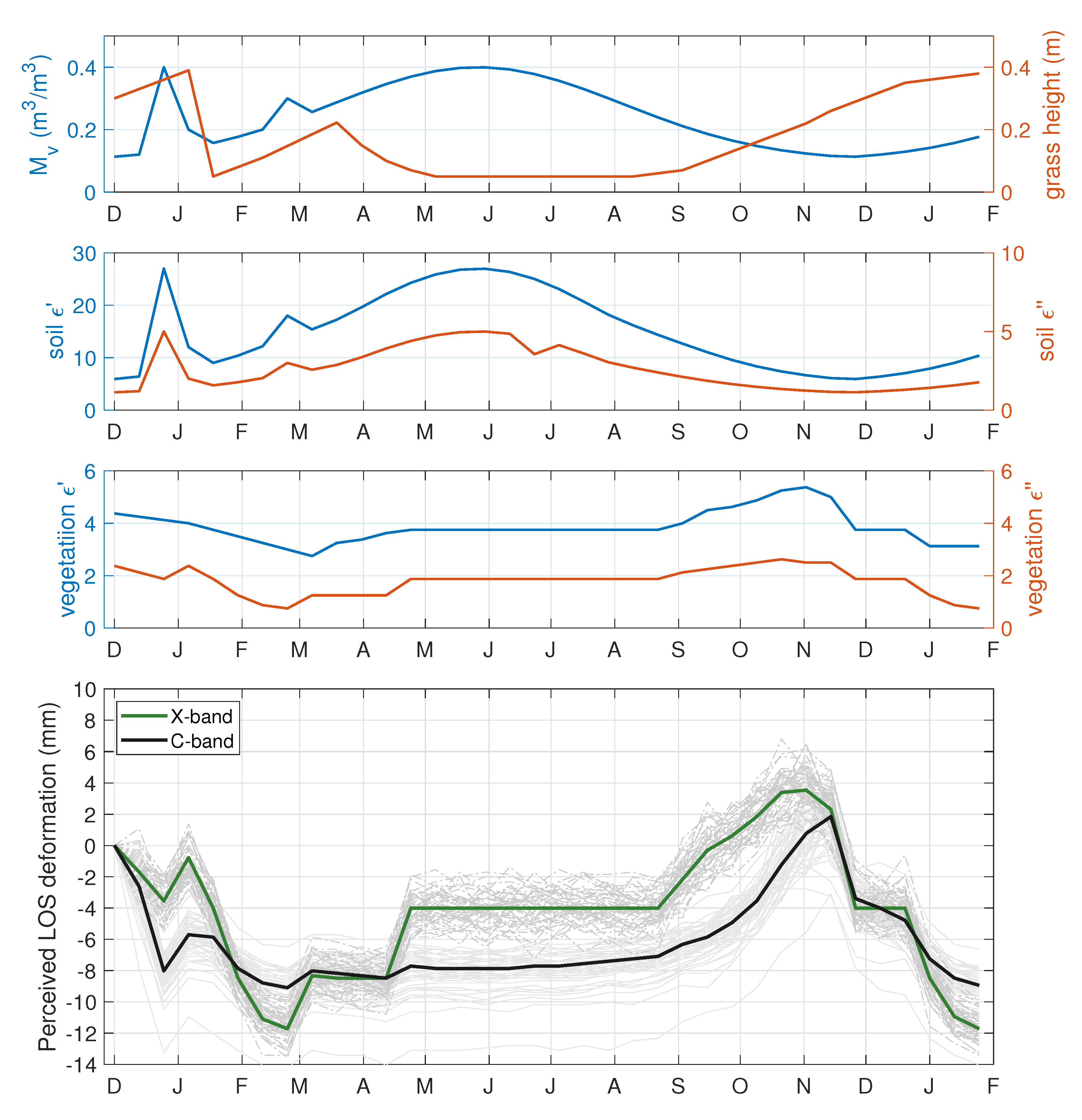
Experiment III was devised in such a way that phase disturbance was calculated over time. First, dielectric properties of the (southern hemisphere) pasture were estimated, changing over the course of 14 months due to varying grass heights, and soil and vegetation moisture (Table 2). This included realistic scenarios such as increased soil and vegetation moisture due to some heavier showers (one in December and one in February), grass and soil drying out over summer (December to March), a grass-cut (January), cattle grazing (March–May), and grass not growing over winter (May–August). Phase differences were calculated to build a synthetic LOS displacement curve over the 14 months, for two commonly used InSAR frequencies, i.e., C-band and X-band (8–10 GHz). Because dielectric properties change with microwave frequency, we assumed slightly different permittivity values for X and C bands. We used the finding of Hallikainen et al. [31] and used the simplified assumption:
Additionally, a 50-member ensemble of slightly varying permittivities (±5%) was used for each frequency in order to sufficiently analyse this experiment’s sensitivity of phase disturbance to small permittivity changes.
3. Findings
3.1. Result Analyses of our Three Experiments
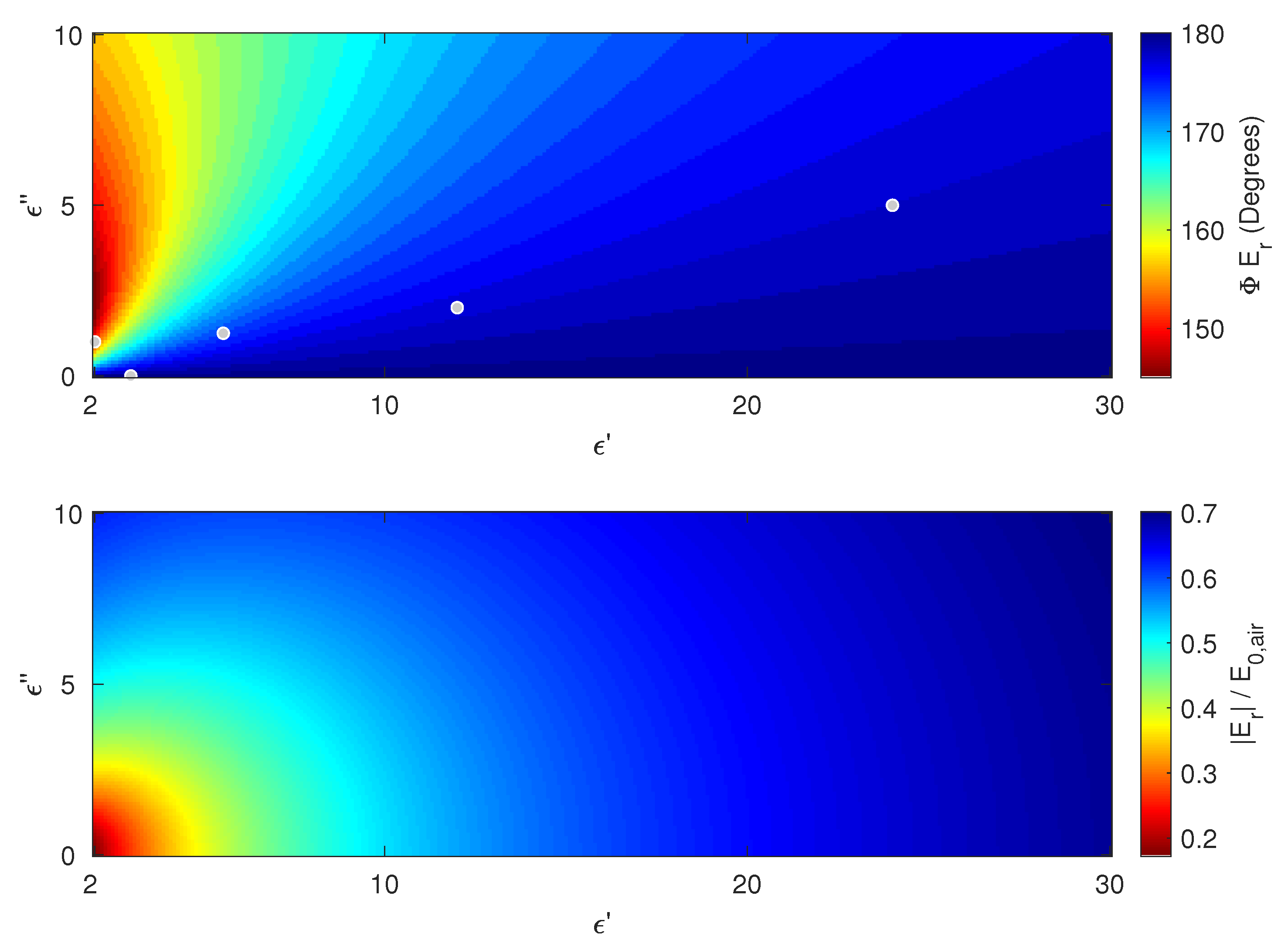
Experiment I (Figure 2 and Table 1) show that reflection from air at another dielectric medium ( = 0) results in a “normal” reflection: the reflected E field reverses by 180 as expected. Reflection from air at a lossy medium can cause a phase disturbance because transmission through the lossy medium results in the H-field lagging the E-field. Since the reflected and transmitted waves have to comply with the boundary conditions of Equation (4) and the ratios between incoming, reflected, and transmitted energy in Equation (6), the reflected wave to the satellite can show a phase disturbance. Most soils have a relatively high , and thus often phase disturbances are negligible in terms of noise on the perceived LOS displacement, i.e., under a mm through this example: the reflected EM field at the interface between air and silty clay shows a phase difference of 2, translating to a very small 0.3 mm in noise in the perceived LOS displacement if this were a C-band EM wave. However, phase disturbances (and amplitude decrease) can be high for small , up to almost a 1 cm (almost 30 degrees of a C-band wave for cases where a soil nears dielectric properties of air, e.g., a slightly wet sand or remnant moisture in grass roots in a dry sand. The largest differences are found for small permittivities and small interferometric permittivity contrasts of the soil. Although this seems counterintuitive (one might expect large differences at a high permittivity contrast), waves travelling between (complex) media can be forced to shift their phase significantly in order to meet the simple boundary conditions Equation (4).
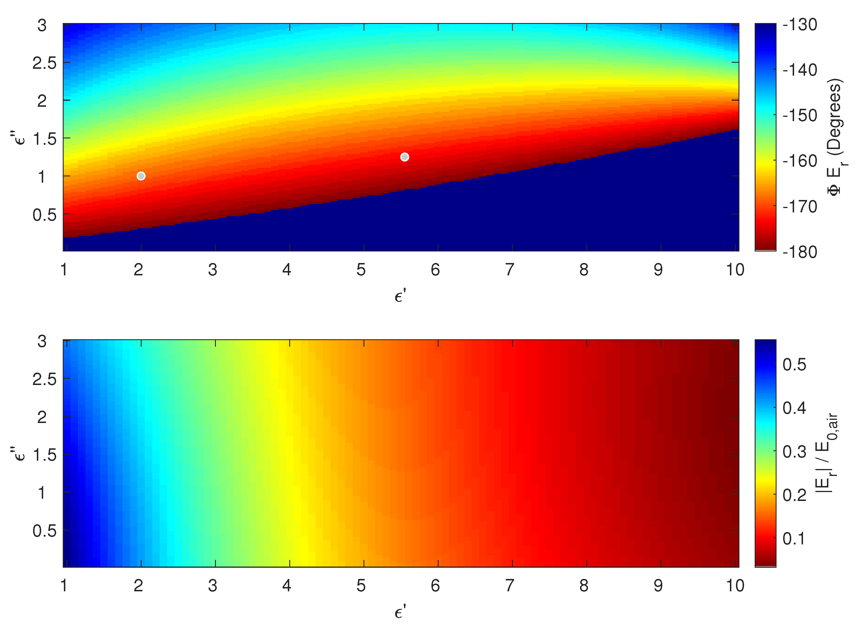
Addition of a vegetation layer to the model (experiment II, Figure 3, Table 1) can theoretically lead to a decrease in amplitude of 70–100% and phase disturbances anywhere between −180 and 180, with most vegetation likely to show phase disturbances between −180 and −130. Phase disturbances of several tens of degrees are significant noise to the perceived LOS displacement and can translate to up to 8-mm interferometric differences (assuming C-band).
A simulated hypothetical 14 months of pasture data (experiment III, Figure 4) show that perceived LOS displacements can contain considerable noise caused by phase disturbances because of the small temporal variations in soil and vegetation dielectric properties. Phase disturbances are most sensitive to changes in vegetation (height and moisture). Both X-band and C-band waves are sensitive to small changes in dielectric properties, resulting in phase disturbances up to more than 1 cm. This confirms our finding that small changes in permittivities might lead to relatively large phase disturbances, as can also be seen by the relatively large spread of the 50 ensemble members that were simulated.
3.2. Comparison to Other Studies
The results of this study reveal that small temporal, seasonal, and sub-seasonal interferometric differences in permittivity of both soil and vegetation can have large effects on phase disturbance (while large differences have a negligible effect). This is a result of the reflection–transmission boundary conditions between two media where permittivity is complex in at least one of the media.
Our results explain the sub-centimetre seasonal phase disturbances found in InSAR studies mentioned in the introduction. For example, Lundgren et al. [3] found long-term patterns of uplift of Mt. Etna, which relates to magmatic inflation, but cannot explain seasonal trends and variations that are in the order of 1 cm or less. Lauknes et al. [20] found seasonal patterns in SBAS data in the autumns of 1996 and 1998, where they cannot explain LOS displacements that suggest a seasonal upwards terrain motion of almost 10 mm. Tomás et al. [22] confirmed that variations of 10 mm in LOS displacement are seasonal. They then related this to change in groundwater level. Reeves et al. [21] surmised, from seasonal variations of InSAR of approximately 1 cm or less, that InSAR might capture seasonal variation of hydraulic heads. They showed high correlation in areas between irrigation circles, where there is little vegetation. They then derived a model of hydraulic head, using the elastic skeletal properties of the subsurface. Our proposed theory suggests that, although the correlation with hydraulic head and the InSAR data might exist, the actual cause of the seasonal variations might well be explained by our phase disturbance model without any surface movement, e.g., in dryland areas with little vegetation. Özer et al. [19] interpreted seasonally occurring phase differences and LOS displacements of levees of up to 1 cm as forthcoming from swelling and shrinkage behaviour, including an underlying deformation behaviour model. Our models find the same magnitude and pattern of deformation, suggesting that phase differences through soil moisture and vegetation characteristics can explain for their LOS displacement.
Our results confirm the observed variations of Brancato and Hajnsek [24], who found that the change in phase disturbance increases with drying biomass. They found differences of only a few degree of phase angle change for drying biomass that is still wet to a quick increase up to more than 0.5 phase angle change for drying biomass that is already quite dry.
The study of De Zan et al. [26] used the same concept we use, i.e., that phase disturbances of microwaves travelling between media are caused by the difference in dielectric properties between these media. They found similar magnitude angles of relative phase disturbance, i.e., a 10-degree maximum change for soil moisture, which is equivalent to approximately 1 mm in the case of a C-band wave. Because our study included both soil moisture and vegetation, we can conclude that phase disturbances are less sensitive to changes in soil moisture and more sensitive to that in vegetation. De Zan et al. [26] took their experiment further, being able to use their findings to invert soil moisture, while our experiments are more for explaining both soil moisture and vegetation as well as for trying to further explain when phase differences might appear. Our recommendation is to combine the findings of this study into other studies, e.g., to incorporate both soil and vegetation in studies like De Zan et al. [26].
4. Discussion
Our research used simplifying assumptions because basic microwave theory is already deemed enough to prove the point of this study, i.e., that the phase disturbance effect of slightly varying dielectric properties of soil, roots, and vegetation on the InSAR signal could be misinterpeted as actual ground deformation and that we hope that this study gives more physics-based explanations to help improve future InSAR land motion interpretation. One might want to elaborate on the theory in our study and to use more advanced models, e.g., to forecast phase disturbances if vegetation and soil properties are precisely known. More advanced models could incorporate more advanced backscatter models, e.g., models that take into account more than only normal incidence. However, we surmise that impractical, since the far bigger issue to be solved is that we cannot estimate permittivity of vegetation and soils with the amount of detail required, especially since our experiments show that phase disturbance is very sensitive to small changes and that very small differences in permittivity can already cause large phase disturbances. Our decision to incorporate a hypothetical “year in a paddock” experiment (III) was merely to better visualise phase disturbances in a more practical (synthetic) InSAR experiment, proving that phase disturbances might be misinterpreted as terrain motion. However, we acknowledge that the estimated soil and vegetation permittivities were theoretical estimates and thus uncertain and coarse. This was another reason for choosing 50-member ensembles.
The noise on PSI-based LOS displacement has not been described in this study (we assumed SBAS or similar studies) and is probably more complex. After all, most PSI measurements come directly from man-made structures and small changes in permittivity of those materials have not been studied for this paper. Furthermore, some PSI measurement can “double bounce” from soil, i.e., they first reflect on soil before reflecting on man-made structures and back to the satellite. Future research could aim towards a similar theory as in this paper but for man-made structures, including double-bounce features.
5. Conclusions
This study has further explored phase disturbances mentioned by De Zan et al. [26] but with inclusion of both soil moisture as well as vegetation. By setting up dedicated experiments, our model calculated phase and amplitude at the boundary of two media, combining fundamental theories of microwave reflection and transmission of normal incident electromagnetic waves. We have found new evidence that small temporal differences in soil moisture and vegetation can have a relatively large effect on microwave phase disturbances and that this effect is dominated by vegetation. These phase disturbances can occur as a result of the boundary conditions at reflection and transmission between two media with different dielectric properties.
The results of our theoretical experiments explain how (sub-)seasonal differences in soil moisture and vegetation on surfaces without any terrain motion are perceived as InSAR LOS displacement. Our findings agree with the InSAR LOS interpretations found in other recent studies; moreover, they explain the seasonal LOS displacements found in several other studies and give an alternative explanation for interpretations of ground deformation in these studies.
We surmise that our findings will be useful for further research, e.g., incorporating this seasonal signature as an alternative explanation to seasonal ground movement; combining the findings of our study with other studies, e.g., [24,26]; and finding more evidence and ground observation in measurement campaigns to further explain these seasonal InSAR signatures.
The Supplementary Materials contain more details of the performed experiments and access to all model scripts that were developed to generate the results.
Supplementary Materials
The following are available online at https://0-www-mdpi-com.brum.beds.ac.uk/2072-4292/12/18/3029/s1, S1: Scripts used to derive the results of this study, S2: Details of InSAR and microwave radar theory.
Author Contributions
R.W. and M.S.-R. conceived and designed the experiments; R.W. performed the experiments and analysed the data; M.S.-R. contributed to reviewing the text and adding microwave reflection and transmission at boundaries. R.W. and M.S.-R. wrote the paper. All authors have read and agreed to the published version of the manuscript.
Funding
This research was part of the Smart Aquifer Characterisation (SAC) Programme, funded by the Ministry of Business, Innovation, and Employment, New Zealand, contract C05X1102. Funds have been made available for covering the costs to publish in open access.
Acknowledgments
This research has been performed as part of a Ph.D. study of the main author at the University of Waikato, New Zealand [39].
Conflicts of Interest
The authors declare no conflict of interest.
References
- Funning, G.J.; Parsons, B.; Wright, T.J.; Jackson, J.A.; Fielding, E.J. Surface displacements and source parameters of the 2003 Bam (Iran) earthquake from Envisat advanced synthetic aperture radar imagery. J. Geophys. Res. Solid Earth 2005, 110. [Google Scholar] [CrossRef] [Green Version]
- Atzori, S.; Antonioli, A.; Tolomei, C.; De Novellis, V.; De Luca, C.; Monterroso, F. InSAR full-resolution analysis of the 2017–2018 M>6 earthquakes in Mexico. Remote Sens. Environ. 2019, 234, 111461. [Google Scholar] [CrossRef]
- Lundgren, P.; Casu, F.; Manzo, M.; Pepe, A.; Berardino, P.; Sansosti, E.; Lanari, R. Gravity and magma induced spreading of Mount Etna volcano revealed by satellite radar interferometry. Geophys. Res. Lett. 2004, 31. [Google Scholar] [CrossRef] [Green Version]
- Pritchard, M.E.; Biggs, J.; Wauthier, C.; Sansosti, E.; Arnold, D.W.D.; Delgado, F.; Ebmeier, S.K.; Henderson, S.T.; Stephens, K.; Cooper, C.; et al. Towards coordinated regional multi-satellite InSAR volcano observations: Results from the Latin America pilot project. J. Appl. Volcanol. 2018, 7, 5. [Google Scholar] [CrossRef]
- Carnec, C.; Fabriol, H. Monitoring and modeling land subsidence at the Cerro Prieto Geothermal Field, Baja California, Mexico, using SAR interferometry. Geophys. Res. Lett. 1999, 26, 1211–1214. [Google Scholar] [CrossRef]
- Carlà, T.; Intrieri, E.; Raspini, F.; Bardi, F.; Farina, P.; Ferretti, A.; Colombo, D.; Novali, F.; Casagli, N. Perspectives on the prediction of catastrophic slope failures from satellite InSAR. Sci. Rep. 2019, 9, 14137. [Google Scholar] [CrossRef] [Green Version]
- Hooijer, A.; Page, S.; Jauhiainen, J.; Lee, W.A.; Lu, X.X.; Idris, A.; Anshari, G. Subsidence and carbon loss in drained tropical peatlands. Biogeosciences 2012, 9, 1053–1071. [Google Scholar] [CrossRef] [Green Version]
- Wu, J.; Shi, X.; Xue, Y.; Zhang, Y.; Wei, Z.; Yu, J. The development and control of the land subsidence in the Yangtze delta, China. Environ. Geol. 2007, 55, 1725–1735. [Google Scholar] [CrossRef]
- Ortega-Guerrero, A.; Rudolph, D.L.; Cherry, J.A. Analysis of long-term land subsidence near Mexico City: Field investigations and predictive modeling. Water Resour. Res. 1999, 35, 3327–3341. [Google Scholar] [CrossRef]
- Chen, J.; Knight, R.; Zebker, H.A. The Temporal and Spatial Variability of the Confined Aquifer Head and Storage Properties in the San Luis Valley, Colorado Inferred From Multiple InSAR Missions. Water Resour. Res. 2017, 53, 9708–9720. [Google Scholar] [CrossRef]
- Hu, X.; Lu, Z.; Wang, T. Characterization of Hydrogeological Properties in Salt Lake Valley, Utah, using InSAR. J. Geophys. Res. Earth Surf. 2018, 123, 1257–1271. [Google Scholar] [CrossRef]
- Ferretti, A.; Prati, C.; Rocca, F. Nonlinear subsidence rate estimation using permanent scatterers in differential SAR interferometry. IEEE Trans. Geosci. Remote Sens. 2000, 38, 2202–2212. [Google Scholar] [CrossRef] [Green Version]
- Berardino, P.; Fornaro, G.; Lanari, R.; Sansosti, E. A new algorithm for surface deformation monitoring based on small baseline differential SAR interferograms. IEEE Trans. Geosci. Remote Sens. 2002, 40, 2375–2383. [Google Scholar] [CrossRef] [Green Version]
- Massonnet, D.; Feigl, K.L. Radar interferometry and its application to changes in the Earth’s surface. Rev. Geophys. 1998, 36, 441–500. [Google Scholar] [CrossRef] [Green Version]
- Hanssen, R.F. Radar Interferometry: Data Interpretation and Error Analysis, 2nd ed.; Remote Sensing and Digital Image Processing; Kluwer Academic: Dordrecht, The Netherlands; Boston, MA, USA, 2001. [Google Scholar]
- Barnhart, W.D.; Lohman, R.B. Characterizing and estimating noise in InSAR and InSAR time series with MODIS. Geochem. Geophys. Geosyst. 2013, 14, 4121–4132. [Google Scholar] [CrossRef]
- Emardson, T.R.; Simons, M.; Webb, F.H. Neutral atmospheric delay in interferometric synthetic aperture radar applications: Statistical description and mitigation. J. Geophys. Res. Solid Earth 2003, 108. [Google Scholar] [CrossRef]
- Hanssen, R.F. Atmospheric Heterogeneities in ERS Tandam SAR Interferometry; Volume Report DUP 98.1; Delft University Press: Delft, The Netherlands, 1998. [Google Scholar]
- Özer, I.E.; Rikkert, S.J.H.; van Leijen, F.J.; Jonkman, S.N.; Hanssen, R.F. Sub-seasonal Levee Deformation Observed Using Satellite Radar Interferometry to Enhance Flood Protection. Sci. Rep. 2019, 9. [Google Scholar] [CrossRef] [Green Version]
- Lauknes, T.; Piyush Shanker, A.; Dehls, J.; Zebker, H.; Henderson, I.; Larsen, Y. Detailed rockslide mapping in northern Norway with small baseline and persistent scatterer interferometric SAR time series methods. Remote Sens. Environ. 2010, 114, 2097–2109. [Google Scholar] [CrossRef]
- Reeves, J.A.; Knight, R.; Zebker, H.A.; Schreüder, W.A.; Shanker Agram, P.; Lauknes, T.R. High quality InSAR data linked to seasonal change in hydraulic head for an agricultural area in the San Luis Valley, Colorado. Water Resour. Res. 2011, 47. [Google Scholar] [CrossRef] [Green Version]
- Tomás, R.; Li, Z.; Lopez-Sanchez, J.M.; Liu, P.; Singleton, A. Using wavelet tools to analyse seasonal variations from InSAR time-series data: A case study of the Huangtupo landslide. Landslides 2016, 13, 437–450. [Google Scholar] [CrossRef] [Green Version]
- Zwieback, S.; Hajnsek, I.; Edwards-Smith, A.; Morrison, K. Depth-Resolved Backscatter and Differential Interferometric Radar Imaging of Soil Moisture Profiles: Observations and Models of Subsurface Volume Scattering. IEEE J. Sel. Top. Appl. Earth Obs. Remote Sens. 2017, 10, 3281–3296. [Google Scholar] [CrossRef]
- Brancato, V.; Hajnsek, I. Analyzing the Influence of Wet Biomass Changes in Polarimetric Differential SAR Interferometry at L-Band. IEEE J. Sel. Top. Appl. Earth Obs. Remote Sens. 2018, 11, 1494–1508. [Google Scholar] [CrossRef]
- Zwieback, S.; Hajnsek, I. Influence of Vegetation Growth on the Polarimetric Zero-Baseline DInSAR Phase Diversity—Implications for Deformation Studies. IEEE Trans. Geosci. Remote Sens. 2016, 54, 3070–3082. [Google Scholar] [CrossRef]
- De Zan, F.; Parizzi, A.; Prats-Iraola, P.; Lopez-Dekker, P. A SAR Interferometric Model for Soil Moisture. IEEE Trans. Geosci. Remote Sens. 2014, 52, 418–425. [Google Scholar] [CrossRef] [Green Version]
- Pain, H. Chapter 8: Electromagnetic Waves. In The Physics of Vibrations and Waves, 6th ed.; John Wiley & Sons, Ltd.: West Sussex, UK, 2005; pp. 199–238. [Google Scholar]
- Ulaby, F.; Moore, R.; Fung, A. Microwave Remote Sensing—Active and Passive; Volume II, Advanced Level Textbooks and Reference Works; Addison-Wesley: Reading, MA, USA, 1982; p. 607. [Google Scholar]
- Böttcher, C.J.F. Dielectrics in Time-Dependent Fields, 2nd ed.; Elsevier Scientific Pub. Co.: Amsterdam, NY, USA, 1978. [Google Scholar]
- Lorrain, P.; Corson, D.R.; Lorrain, F. Electromagnetic Fields and Waves: Including Electric Circuits, 3rd ed.; Freeman: New York, NY, USA, 1988. [Google Scholar]
- Hallikainen, M.T.; Ulaby, F.T.; Dobson, M.C.; El-Rayes, M.A.; Wu, L.K. Microwave dielectric behavior of wet soil-part 1: Empirical models and experimental observations. IEEE Trans. Geosci. Remote Sens. 1985, 1, 25–34. [Google Scholar] [CrossRef]
- Gadani, D.; Rana, V.; Bhatnagar, S.; Prajapati, A.; Vyas, A. Effect of salinity on the dielectric properties of water. Indian J. Pure Appl. Phys. (IJPAP) 2012, 50, 405–410. [Google Scholar]
- Ellison, W.; Balana, A.; Delbos, G.; Lamkaouchi, K.; Eymard, L.; Guillou, C.; Prigent, C. New permittivity measurements of seawater. Radio Sci. 1998, 33, 639–648. [Google Scholar] [CrossRef]
- El-rayes, M.; Ulaby, F. Microwave Dielectric Spectrum of Vegetation—Part I: Experimental Observations. IEEE Trans. Geosci. Remote Sens. 1987, GE-25, 541–549. [Google Scholar] [CrossRef]
- Ulaby, F.; Tavakoli, A.; Thomas, B. Microwave Propagation Constant for a Vegetation Canopy With Vertical Stalks. IEEE Trans. Geosci. Remote Sens. 1987, GE-25, 714–725. [Google Scholar] [CrossRef]
- Dobson, M.; Ulaby, F.; Hallikainen, M.; El-rayes, M. Microwave Dielectric Behavior of Wet Soil—Part II: Dielectric Mixing Models. IEEE Trans. Geosci. Remote Sens. 1985, GE-23, 35–46. [Google Scholar] [CrossRef]
- Xian, C.L.; Chen, Y.; Tong, L.; Jia, M.Q. Measurement on the Dielectric Constant of Grass with Rectangular Waveguide at C Band. Appl. Mech. Mater. 2011, 130–134, 2138–2142. [Google Scholar] [CrossRef]
- Attema, E.P.W.; Ulaby, F.T. Vegetation modeled as a water cloud. Radio Sci. 1978, 13, 357–364. [Google Scholar] [CrossRef]
- Westerhoff, R. Satellite Remote Sensing for Improvement of Groundwater Characterisation. Ph.D. Thesis, University of Waikato, Hamilton, NZ, USA, 2017. [Google Scholar]
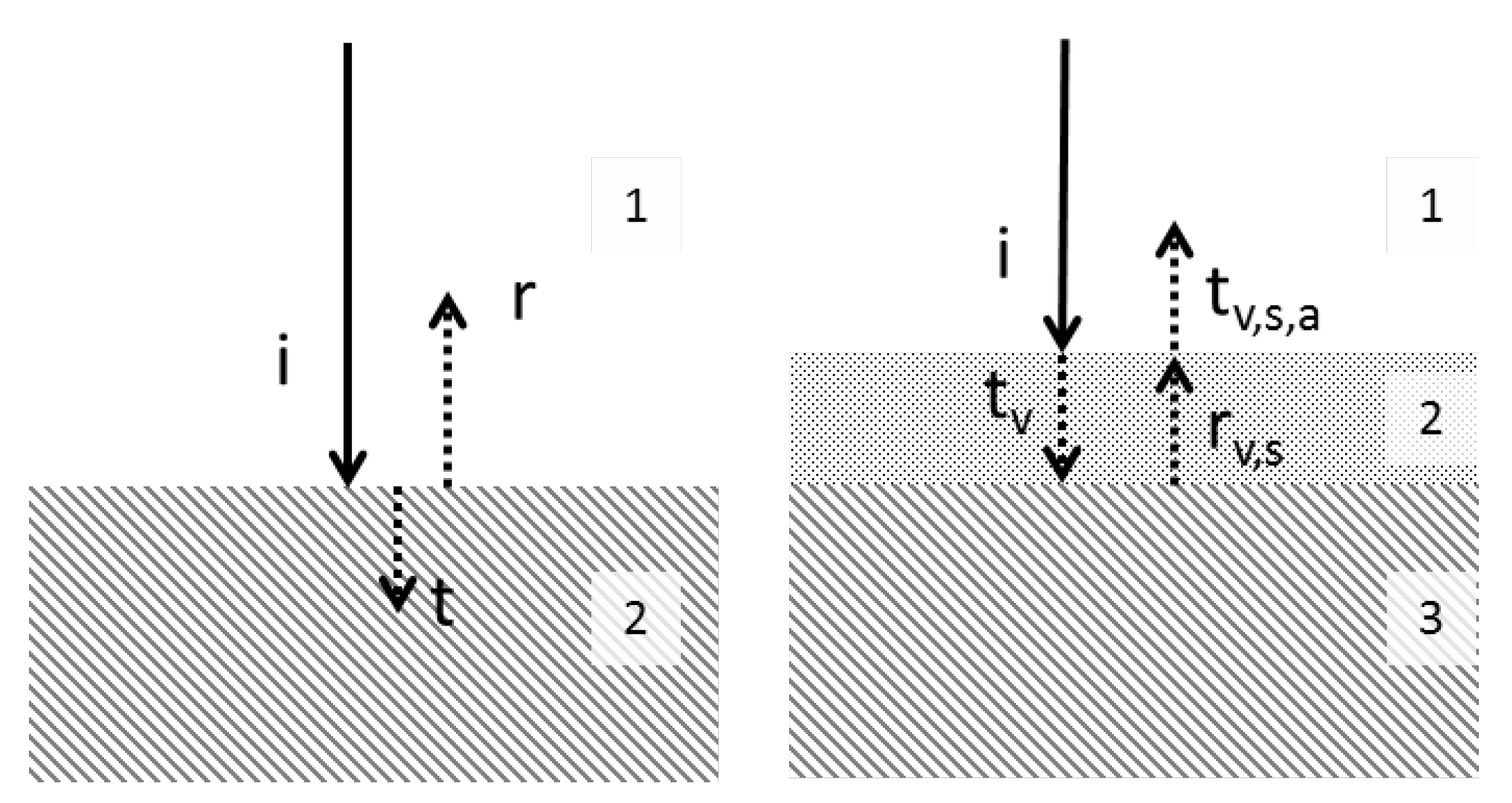
Figure 1.
(Left) schematics of experiment I of the incoming (i), transmitted (t), and reflected (r) energy between medium 1 (typically air) and medium 2 (soil or vegetation). (Right) schematics of experiment II, with three media (1 = air, 2 = vegetation, and 3 = soil) with “t” as the transmitted energy from air to vegetation, “r” as the reflected energy from vegetation to soil, and ”t” as the transmitted energy from vegetation to air (i.e., back to the satellite). Transmitted energy from vegetation to soil and direct reflection from air to vegetation are not shown.

Figure 2.
Phase (top) and amplitude (bottom) of the reflected E field , relative to the incoming signal (), for a range of complex permittivities ( and ) of bare soil: permittivities of Table 1 are plotted as gray circles in the top-left image.
Figure 2.
Phase (top) and amplitude (bottom) of the reflected E field , relative to the incoming signal (), for a range of complex permittivities ( and ) of bare soil: permittivities of Table 1 are plotted as gray circles in the top-left image.

Figure 3.
Phase (top) and amplitude (bottom) of the reflected E field , relative to the incoming signal (), for a range of complex permittivities ( and ) of vegetation: vegetation permittivities of Table 1 are plotted in gray circles in the top image. Underlying soil is assumed to be a sandy loam with soil moisture = 0.2 mm. The top figure shows a dark blue triangle, representing the E-field that has undergone phase disturbances that include a 180 phase shift.

Figure 4.
Hypothetical values of soil moisture (), grass height, and soil and vegetation permittivities (for C-band) over 14 months in a pasture without terrain motion (the top three plots) and the resulting synthetic perceived LOS deformation through phase disturbances (bottom plot) of C-band and X-band microwave radar: our “year in a paddock” included realistic scenarios of southern hemisphere pasture with (sub-)seasonal changes in soil and vegetation moisture due to some heavier showers (December and March), grass and soil drying out over summer (December to March), a grass-cut (January), cattle grazing (March–May), and grass not growing over winter (May–August).


Table 1.
Approximate dielectric properties for some of Earth’s materials at normal pressure and temperature [31,32,33,34,35,36,37] and results of experiments I and II. is soil moisture with unit m m.
| Material | Exp. I: () | Exp. II: () | ||
|---|---|---|---|---|
| Air | ≈1 | 0 | - | - |
| Pure Water | 75 | 15 | - | - |
| Fresh-Brackish Water (<5000 ppm) | 75 | 30 | - | - |
| Dry sand | 3 | 0 | 180 | - |
| Sandy loam ( = 0.2) | 12 | 2 | 177 | - |
| Silty Clay ( = 0.4) | 24 | 5 | 178 | - |
| Crop Vegetation example | 5.5 | 1.25 | 174 | −173 |
| Grass vegetation example | 2 | 1 | 151 | −168 |
Table 2.
Material properties at C-band microwave frequencies of the “pasture over a year” experiment. = soil moisture; = vegetation. Conversion to X-band dielectric properties was performed using Equation (8).
Table 2.
Material properties at C-band microwave frequencies of the “pasture over a year” experiment. = soil moisture; = vegetation. Conversion to X-band dielectric properties was performed using Equation (8).
| Date [dd/mm/yyyy] | [mm] | Grass Height [m] | Description | ||||
|---|---|---|---|---|---|---|---|
| 1/12/2012 | 0.11 | 5.9 | 1.1 | 0.3 | growing | 4.4 | 2.4 |
| 13/12/2012 | 0.12 | 6.4 | 1.2 | 0.33 | growing | 4.33 | 2.135 |
| 25/12/2012 | 0.4 | 27 | 5 | 0.36 | growing | 4.13 | 1.88 |
| 6/01/2013 | 0.2 | 12 | 2 | 0.39 | growing | 4 | 2.38 |
| 18/01/2013 | 0.16 | 9.0 | 1.6 | 0.05 | cut | 3.75 | 1.88 |
| 30/01/2013 | 0.18 | 10.4 | 1.8 | 0.08 | drying out | 3.5 | 1.25 |
| 11/02/2013 | 0.20 | 12.2 | 2.0 | 0.11 | drying out | 3.25 | 0.88 |
| 23/02/2013 | 0.3 | 18.0 | 3 | 0.15 | drying out | 3 | 0.75 |
| 7/03/2013 | 0.26 | 15.4 | 2.6 | 0.185 | growing | 2.75 | 1.25 |
| 19/03/2013 | 0.29 | 17.2 | 2.9 | 0.2225 | growing | 3.25 | 1.25 |
| 31/03/2013 | 0.32 | 19.6 | 3.4 | 0.15 | grazing | 3.375 | 1.25 |
| 12/04/2013 | 0.35 | 22.1 | 3.9 | 0.1 | grazing | 3.63 | 1.25 |
| 24/04/2013 | 0.37 | 24.3 | 4.4 | 0.07 | winter | 3.75 | 1.88 |
| 6/05/2013 | 0.39 | 25.8 | 4.8 | 0.05 | winter | 3.75 | 1.88 |
| 18/05/2013 | 0.40 | 26.8 | 5.0 | 0.05 | winter | 3.75 | 1.88 |
| 30/05/2013 | 0.40 | 27.0 | 5.0 | 0.05 | winter | 3.75 | 1.88 |
| 11/06/2013 | 0.39 | 26.4 | 4.9 | 0.05 | winter | 3.75 | 1.88 |
| 23/06/2013 | 0.38 | 25.0 | 3.6 | 0.05 | winter | 3.75 | 1.88 |
| 5/07/2013 | 0.36 | 23.1 | 4.1 | 0.05 | winter | 3.75 | 1.88 |
| 17/07/2013 | 0.33 | 20.7 | 3.6 | 0.05 | winter | 3.75 | 1.88 |
| 29/07/2013 | 0.30 | 18.2 | 3.0 | 0.05 | winter | 3.75 | 1.875 |
| 10/08/2013 | 0.27 | 16.2 | 2.7 | 0.05 | winter | 3.75 | 1.88 |
| 22/08/2013 | 0.24 | 14.4 | 2.4 | 0.06 | winter | 3.75 | 1.88 |
| 3/09/2013 | 0.21 | 12.7 | 2.1 | 0.07 | winter | 4 | 2.13 |
| 15/09/2013 | 0.19 | 11.0 | 1.9 | 0.1 | growing | 4.5 | 2.25 |
| 27/09/2013 | 0.17 | 9.6 | 1.7 | 0.13 | growing | 4.63 | 2.375 |
| 9/10/2013 | 0.15 | 8.3 | 1.5 | 0.16 | growing | 4.88 | 2.5 |
| 21/10/2013 | 0.13 | 7.4 | 1.3 | 0.19 | growing | 5.25 | 2.63 |
| 2/11/2013 | 0.12 | 6.6 | 1.2 | 0.22 | growing | 5.38 | 2.5 |
| 14/11/2013 | 0.12 | 6.1 | 1.2 | 0.26 | growing | 5 | 2.5 |
| 26/11/2013 | 0.11 | 5.9 | 1.1 | 0.29 | growing | 3.75 | 1.88 |
| 8/12/2013 | 0.12 | 6.4 | 1.2 | 0.32 | growing | 3.75 | 1.88 |
| 20/12/2013 | 0.13 | 7.0 | 1.3 | 0.35 | growing | 3.75 | 1.88 |
| 1/01/2014 | 0.14 | 7.9 | 1.4 | 0.36 | growing | 3.13 | 1.25 |
| 13/01/2014 | 0.16 | 9.0 | 1.6 | 0.37 | growing | 3.13 | 0.88 |
| 25/01/2014 | 0.18 | 10.4 | 1.8 | 0.38 | growing | 3.13 | 0.75 |
© 2020 by the authors. Licensee MDPI, Basel, Switzerland. This article is an open access article distributed under the terms and conditions of the Creative Commons Attribution (CC BY) license (http://creativecommons.org/licenses/by/4.0/).
Share and Cite
MDPI and ACS Style
Westerhoff, R.; Steyn-Ross, M. Explanation of InSAR Phase Disturbances by Seasonal Characteristics of Soil and Vegetation. Remote Sens. 2020, 12, 3029. https://0-doi-org.brum.beds.ac.uk/10.3390/rs12183029
AMA Style
Westerhoff R, Steyn-Ross M. Explanation of InSAR Phase Disturbances by Seasonal Characteristics of Soil and Vegetation. Remote Sensing. 2020; 12(18):3029. https://0-doi-org.brum.beds.ac.uk/10.3390/rs12183029
Chicago/Turabian StyleWesterhoff, Rogier, and Moira Steyn-Ross. 2020. "Explanation of InSAR Phase Disturbances by Seasonal Characteristics of Soil and Vegetation" Remote Sensing 12, no. 18: 3029. https://0-doi-org.brum.beds.ac.uk/10.3390/rs12183029
Note that from the first issue of 2016, this journal uses article numbers instead of page numbers. See further details here.