Integrating Landsat Time Series Observations and Corona Images to Characterize Forest Change Patterns in a Mining Region of Nanjing, Eastern China from 1967 to 2019

Abstract

Long-term surface mining and subsequent vegetation recovery greatly alter land cover types, reshape landscape patterns and impose several impacts on local ecosystem services. However, studies on the history of forest changes in mining areas from the 1960s to the present have not been reported. This study developed a new idea to investigate the spatial and temporal dynamics of forest cover in a mining area of Mufu Mountain (Mt. Mufu) from 1967 to 2019 by integrating Landsat and Corona data, and to explore the relationships among the forest changes, landscape structures and ecosystem functions. Firstly, we applied the vegetation change tracker (VCT) algorithm and visual interpretation to create annual forest change datasets. Subsequently, the forest loss process was divided into subdivision, shrinkage, perforation and attrition components. An improved forest restoration model in this study extended the recovery process to bridge, branch, infilling and increment components. Finally, remote sensing variables and crown density were coupled to assess the forest aboveground biomass (AGB) to reflect the ecosystem function in the restoration area. Results showed that the combined use of Corona and the dense time series of Landsat can provide more detailed information on forest changes. Forest cover sharply decreased from 343.89 in 1967 to 298.44 ha in 1990, and after 2003, the forest area substantially increased and finally reached a maximum of 434.16 ha in 2019. Subdivision and bridge not only occupied the larger areas in the process of forest loss and restoration, but also they had strong correlations with forest changes and the Pearson correlation coefficients (r) were respectively 0.96 and 0.91. These all revealed that forest changes mainly affected landscape structure connectivity. The total forest AGB of Mt. Mufu increased from 20,173.35 in 2006 to 31,035.77 t in 2017, but the increases in AGB were only 30-40 t/ha in most recovery areas with high structure connectivity (bridge regions), indicating there is room for improving restoration projects in the future. The obtained findings can provide mining site restoration managers with clear, long-term forest change information and mine restoration assessment methods.

1. Introduction

Deforestation, the subsequent increase in degraded landscapes and the resulting loss of forest ecological functions are some of the most severe environmental challenges [1,2,3]. Among the deforestation impacts, surface mining directly changes the land cover, reduces the connectivity at the landscape level and finally leads to adverse environmental impacts and social problems, including loss of biodiversity, vegetation degradation and land occupation [4,5,6,7]. To alleviate the deterioration of landscape patterns and restore the ecological services of ecosystems, an increasing number of mining sites are adopting cleaner production techniques, such as revegetation and mine rehabilitation, to ease the ecological pressure caused by mining [8,9,10]. Therefore, quantifying and analyzing the spatio-temporal dynamics of forest cover, clarifying the landscape spatial process and assessing the ecosystem functions of restored mining areas can help decision makers evaluate the restoration progress of the mining area, draw lessons from the past and propose reasonable management strategies.

Traditional field measurement methods to dynamically monitor mining sites are usually restricted to small areas, and the time frequency of monitoring is low, which leads to an incomplete understanding of forest loss and recovery processes [11]. In recent decades, remote sensing technology has been considered an effective tool for forest change detection [10,12,13,14]. Certain studies have applied the technique to forest cover monitoring in opencast mining areas, which can be summarized into three categories: (1) Spatio-temporal analysis [6,10,15]. These studies aimed to analyze the location and time of forest changes in mining areas based on automated or semi-automated algorithms. For example, Yang et al. [10] adopted the LandTrendr algorithm to detect the spatial extent and change magnitude of the forest cover at a coal mine site in Australia. (2) Landscape pattern analysis [3,14,16,17]. These investigations analyzed the changes in landscape patterns, such as landscape structure and configuration. Sonter et al. [14] examined the land use change in Brazil’s Iron Quadrangle mining region. Wang et al. [16] identified landscape-critical areas around surface mines. (3) Assessment of vegetation restoration projects and their impacts on ecological services [18,19,20]. De Simoni and Praca Leite [18] evaluated the results of 20-year environmental restoration projects in gold mines through soil erosion and stability, vegetation and water body indices. Wang et al. [19] analyzed the impacts of long-term mining disturbance and progressive rehabilitation on ecosystem services, including carbon sequestration, air quality regulation, soil conservation and water yield.

Most of these studies only relied on one sensor with a high time resolution (Landsat or the Moderate Resolution Imaging Spectroradiometer) to provide information on the continuous forest changes in mining areas, and these studies usually began as early as the 1970s. However, certain large-scale land cover changes occurred before this period in many parts of the world [21,22], resulting in inadequate forest change information acquisition. With the declassification of Corona data in 1995, this problem was solved because the Corona satellite program collected more than 800,000 images of Earth’s surface from 1960 to 1972 and allowed information extraction at a fine spatial resolution (1.83–2.74 m) [23,24]. Thus, the combined use of Corona data and Landsat time series further widens the above time span and enables us to obtain rich historical forest cover change information from the 1960s to the present, which is the underlying basis for us to better understand land use management, particularly the suitability of adopted forest management approaches.

Forest cover changes usually bring a series of consequences to the forest landscape pattern. However, the above analysis of the landscape pattern in the mining areas often focused on the forest landscape at certain time points, and ignored the spatial process of forest loss or restoration in the mining area and rarely reported the impacts of forest change on the landscape spatial structure. Generally speaking, the forest loss process can be divided into perforation, subdivision, shrinkage and attrition [25]. The forest recovery process can be classified as increment and expansion [26]. However, the only two categories of the forest recovery process are not enough to completely describe the spatial process of forest recovery. Therefore, the categories describing the forest restoration process in this study can be expanded to infilling, branch, bridge and increment. In this case, the improved model could illustrate the ecological effects of forest restoration. For example, the increment component adds new and small forest patches, but it may make the forest more isolated. The infilling component fills the forest interior to reduce forest edge effects. The branch and bridge components increase the structure connectivity.

The performance of restoration projects should not only consider their impact on the landscape structure, but also it should analyze the ecological function changes of the study area. Although a variety of functional indicators have been applied in many regions to evaluate ecological services [18,19], there are very few examples of attempts to predict forest aboveground biomass (AGB) to investigate the recovery progress and the relationships between structure and function in a mining area. The AGB is essential for the assessment of ecological services and it can reflect the function of forest ecosystems [27,28,29]. Currently, AGB assessment based on remote sensing has been widely used in various studies [28,29]. However, relying solely on remote sensing attributes, the AGB model accuracy remains to be improved. The crown density is an important factor reflecting the forest structure, and it is always highly related to the AGB [30]. Therefore, this study attempts to consider the crown density in the biomass estimation model to improve the accuracy.

To the best of our knowledge, there have been few researches on long-term forest cover and landscape changes in mining areas since the 1960s. In this study, we selected Mufu Mountain (Mt. Mufu) as the research area and aimed to integrate different sensors to characterize the spatial and temporal dynamics of forest cover over the past 52 years (1967–2019). Besides, we provided a different idea to explore the relationships among the forest cover, landscape structure and ecological function. Specifically, (1) based on Landsat and Corona data, we monitored the temporal and spatial change histories of the forest from 1967 to 2019; (2) the forest loss process model and improved recovery process model were adopted to describe the spatial processes of the forest dynamics and statistical analysis was used to investigate the effects of forest changes on the landscape structure; and (3) the forest AGB was predicted to evaluate the progress of the forest restoration project and a quantitative analysis was performed to explore the relationships between ecological function and landscape structure.

2. Materials and Methods

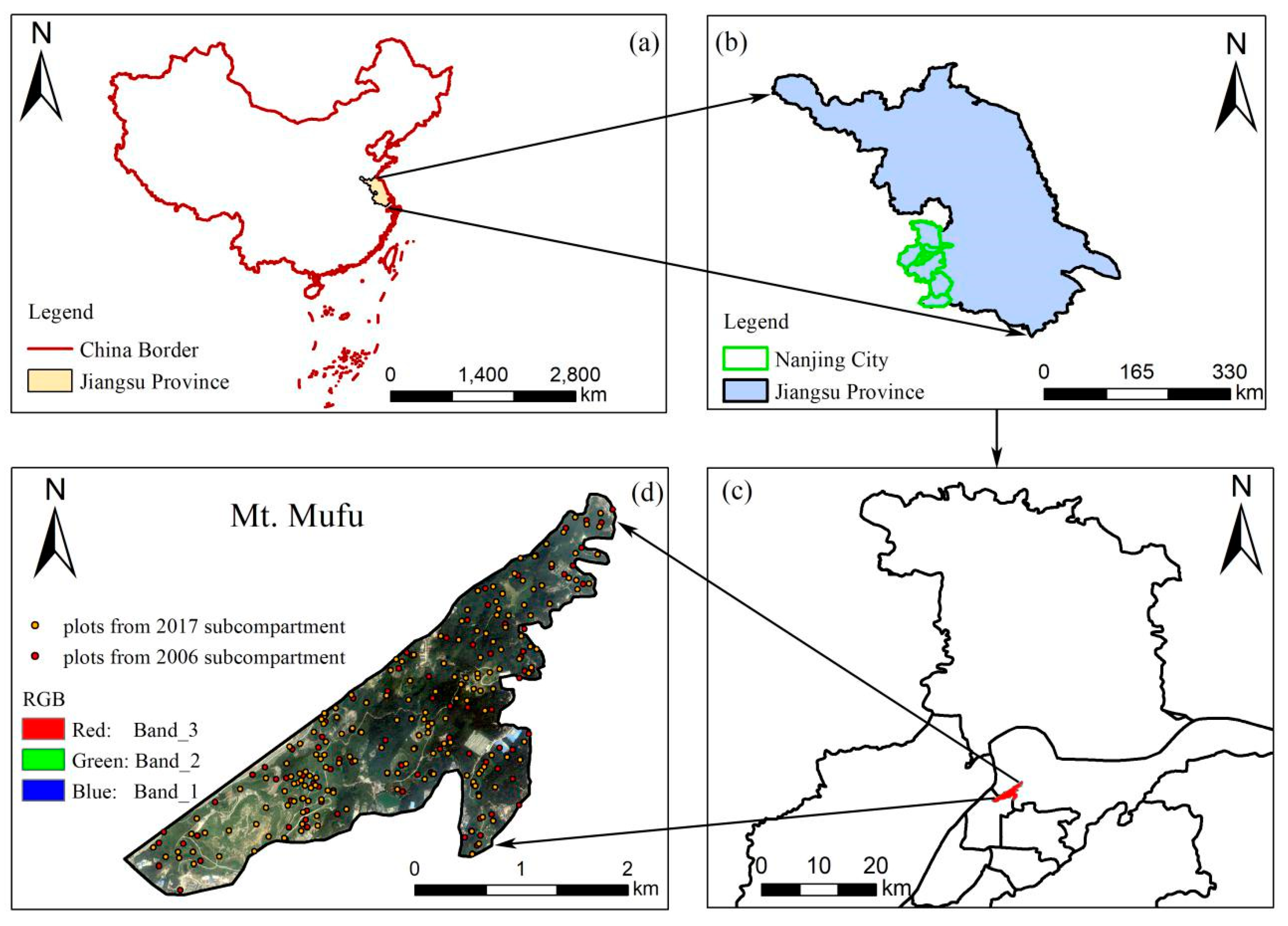
2.1. Study Site

Mt. Mufu is located in northern Nanjing City, Jiangsu Province, China (118°45′52″–118°48′48″E, 32°06′56″–32°08′54″N) and lies along the southern bank of the Yangtze River (Figure 1). Its climate is a humid northern subtropical climate. The mean annual temperature is approximately 15.5°C, and the annual average rainfall ranges from 800 to 1000 mm. Evergreen and deciduous broad-leaved mixed forms are the main forest types [31,32]. Mt. Mufu was a famous area known for its diverse natural and human landscapes. However, because of the growing demand for building materials from industry and urban construction, mining was started on Mt. Mufu in the mid-20th century due to its abundant dolomite and limestone. As a result, the natural vegetation was seriously damaged [33]. In 1999, the Nanjing government closed quarries and started vegetation recovery projects in mine regions.

2.2. Study Data

2.2.1. Remote Sensing Data and Processing

The data analyzed in this study included Corona data, Landsat images and digital elevation model (DEM) data. Corona satellites used panoramic cameras to obtain photographs of Earth’s surface between 1960 and 1972. These photographs are 8-bit panchromatic images with a high spatial resolution and were originally used for reconnaissance by the United States intelligence agencies. Since Corona data are no longer important to national security, these images were declassified in 1995 [24]. To ensure the accuracy of change detection, Corona data should be collected during the summer if possible. The Corona data in this study were from the Key Hole (KH) 4A and 4B missions in 1967 and 1970, respectively, and the resolution was 2.74 and 1.83 m, respectively (

Table 1. Remote sensing data used in this study.

Source	Mission	Resolution (m)	Date/type
USGS	KH-4A	2.74	19670802
	KH-4B	1.83	19700525
	TM	30	19870921, 19880705, 19900711, 19910831, 19921020, 19930617, 19940722, 19951013, 19970831, 19980615, 19990618, 20020712, 20030731, 20051008, 20060520, 20070726, 20091003, 20100819, 20110518
	ETM+	30	20000916, 20010717
	OLI	30	20130811, 20140611, 20150902, 20160429, 20170721, 20180606, 20190913
NASA	SRTM	90	DEM

). The Landsat data included 28 images from the Landsat 5 Thematic Mapper (TM), Landsat 7 Enhanced Thematic Mapper Plus (ETM+) and Landsat 8 Operational Land Imager (OLI) (path 120/row 38; cloud cover ≤ 10) from 1987 to 2019. We directly obtained atmospherically and geometrically corrected surface reflectance and brightness temperature data from the United States Geological Survey (USGS) (https://glovis.usgs.gov). To accurately map forest changes, the acquisition dates of the Landsat data were also in the vegetation growing season (May to September). DEM data were from the NASA Shuttle Radar Topographic Mission (SRTM) to implement subsequent ortho-rectification. A detailed description of the remote sensing data is provided in Table 1.

The downloaded Corona data only provided rough coordinates of image corners, and they likely contained locational errors of several kilometers [22]. To obtain accurate forest change information, additional ortho-rectification was required for the region of interest [34]. We performed ortho-rectification based on the rational function model, and this ortho-rectification method requires rational polynomial coefficients (RPC). RPC are used to establish the geometric relationship between the plane coordinates of the pixel and the corresponding ground point spatial coordinates. However, the original Corona data lack RPC. Thus, we need to customize RPC. RPC were generated by setting camera parameters and selecting ground control points (GCPs) with DEM data to establish external orientation parameters [34]. The camera parameters, such as focal length and film resolution, can be obtained from Altmaier and Kany [34] and Galiatsatos [35]. Ground control points were selected by looking for common points in Corona and high-resolution Google Earth images (with the same spatial reference as Landsat) and these control points included road intersections, urban city structures and other stable ground features. Subsequently, we conducted the ortho-rectification using the customized RPC. All ortho-rectification steps were completed in the professional software The Environment for Visualizing Images (ENVI).

2.2.2. Field Survey Data and Processing

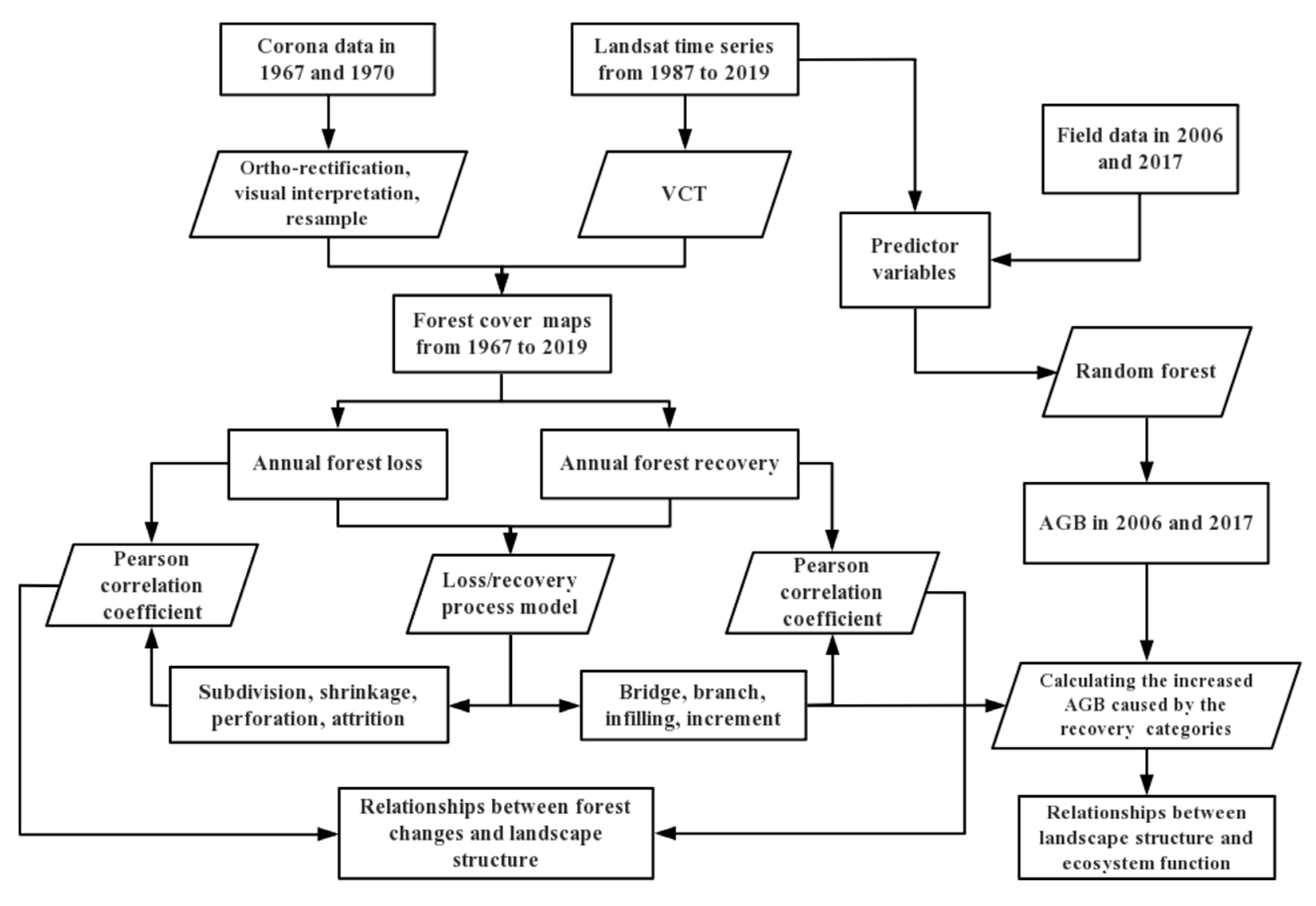
Mt. Mufu’s forest management planning inventory (FMPI) [36,37]—the second level of China’s forest inventory system—was conducted in 2006 and 2017. This type of data divides the forest areas into multiple subcompartments and stores them in vector form. Based on simple visual estimations and angle-gauge sampling, the investigator recorded a bunch of forest characteristics in each subcompartment, including the dominant tree species, origin, crown density, age, site quality, average forest height, average diameter at breast height, stocking volume per unit area, slope and aspect. There were 104 subcompartments in 2006, and 187 subcompartments in 2017 (

Table 2. Basic information of the field survey data in 2006 and 2017.

	Crown Density	Subcompartment (No.)	Minimum AGB (t/ha)	Maximum AGB (t/ha)	Mean AGB (t/ha)	Standard Deviation AGB (t/ha)
2006	≤0.5	48	10.95	23.7	23.38	11.19
	0.6–0.7	52	16.10	110.07	66.06	31.15
	0.8–0.9	4	34.97	115.11	77.51	38.54
2017	≤0.5	13	17.05	39.87	27.83	7.73
	0.6–0.7	140	29.38	143.46	67.01	33.34
	0.8–0.9	34	44.31	199.15	85.37	34.07

) and these plots from subcompartments in 2006 and 2017 were evenly distributed in the study area (Figure 1d). We first adopted the biomass conversion factor method [38,39] to convert the stocking volume into the forest AGB according to different dominant species in each subcompartment (Table S1, Supplementary Materials). The maximum AGB was 115.11 t/ha in 2006, and the maximum AGB was 199.15 t/ha in 2017 (Table 2). To incorporate the crown density into the subsequent AGB modeling, the polygon crown density was converted into raster images as the predicted variable. We adopted the sample function of the R software to perform sampling, and set the sampling probability of each element to 0.8 and 0.2 for model training and validation.

2.3. Method

Visual interpretation of the ortho-rectified Corona data was done to derive forest cover maps in 1967 and 1970 based on available local knowledge. Landsat images were fed into the vegetation change tracker (VCT) algorithm to obtain the forest cover maps from 1987 to 2019. VCT is an automated analysis algorithm based on the spectral-temporal characteristics of the forest change process in the time series to reconstruct the forest disturbance and recovery history. Then, the loss/recovery process models were applied to the forest loss and recovery maps to get the corresponding process categories. Next, remote sensing data from Landsat were combined with two-year field data to evaluate the dynamics of AGB for 2006 and 2017. Finally, statistical analysis and quantitative analysis were utilized to determine the relationships among forest changes, landscape structure and ecosystems function. The overall framework of the current analysis is summarized in Figure 2.

2.3.1. Mapping Forest Cover from the Landsat Observations

The automated VCT model developed by Huang et al. [12] was applied to track the forest changes. Disturbances were determined by detecting deviations in certain vegetation indices, termed the integrated forest z-score (IFZ) in the time series. Its principle is that a forest pixel has a low IFZ, generally less than 3. If a pixel always maintains a low IFZ throughout the observation period, the pixel is then considered a persistent forest pixel. If in a certain year, the IFZ sharply increases, and this increase lasts for several years, this pixel has likely experienced disturbance. If the IFZ of a disturbed pixel slowly decreases, the pixel is returning to a forest pixel. Thus, one of the VCT outputs is the annual forest disturbance map with seven classes (background, persistent water, persistent forest, probable forest with recent disturbance, persistent non-forest, post-disturbance non-forest and disturbed in this year) (

Table 3. Reclassification of the annual forest disturbance maps derived from the vegetation change tracker (VCT) model.

Value	Class Description in the VCT Model	Reclassification
0	Background	Non-forest
1	Persistent non-forest	Non-forest
2	Persistent forest	Forest
4	Persistent water	Non-forest
5	Probable forest with recent disturbance	Forest
6	Disturbed in this year	Non-forest
7	Post-disturbance	Non-forest

). The annual forest disturbance map mainly records the location and area of forest disturbances that occurred in the current year, in addition to persistent and restoration forests. The detailed implementation steps of the VCT algorithm are described in Huang et al. [12].

In this study, we obtained 28 annual disturbance maps from VCT, and for the subsequent forest cover and landscape analysis, we reclassified each disturbance map to obtain a forest cover product from 1987 to 2019. Table 3 lists the criteria for this reclassification. Values 2 (persistent forest) and 5 (probable forest with recent disturbance) were grouped into a new forest class. The remaining classes were reclassified into the non-forest class.

2.3.2. Mapping Forest Cover from the Corona Data

Visual interpretation of the ortho-rectified Corona images was used to derive forest covers in 1967 and 1970 due to (1) the panchromatic Corona images containing limited spectral information, which makes automated pixel-based classification difficult [40]; (2) the images having a sufficiently high spatial resolution to observe the forest and non-forest areas in the study area; and (3) us being very familiar with Mt. Mufu, and therefore we visually determined the forest and non-forest areas by the gray-level tone, shape and texture information of the images in combination with our local knowledge. Finally, the forest cover images were downsampled or aggregated to 30 m resolution by considering the area-dominated criterion (majority rule) [22]. Some narrow road information may be lost during the downsampling. Once done, the resampled forest covers from Corona data were overlaid with those from Landsat to quantify forest cover changes from 1967 to 2019.

2.3.3. Accuracy Assessment of the Forest Cover

Due to the lack of historically archived land use data, we could not validate the forest products of 1967 and 1970 generated via visual interpretation. Huang et al. [12] evaluated the overall accuracy of forest disturbance events determined with the VCT algorithm as approximately 80%. The VCT algorithm accuracy for Nanjing was reported by Li et al. [32] and Zhang et al. [41]. Specifically, Li et al. [32] applied the VCT algorithm to the Ningzhen Mountains of Nanjing, and their results showed that the forest disturbance mapping accuracy ranged from 75% to 85%. Zhang et al. [41] also applied the VCT algorithm to all of Nanjing and found that the overall forest cover mapping accuracy was approximately 88%–92%. These studies have shown that the VCT algorithm is effective and reliable in forest cover and disturbance mapping. Therefore, field survey data and forest cover maps in 2006 and 2017 were exploited to obtain the producer, user and overall accuracies to validate the forest cover products. Producer accuracy refers to the ratio of the correctly classified samples to the samples on the real map for a certain category. User accuracy refers to the ratio of the samples correctly classified to the samples on the classified image for a certain category. Overall accuracy refers to the ratio of the samples correctly classified to the total samples for all categories [42]. For the remaining years, we did not validate the mapping accuracy because we adequately trusted the performance of the VCT algorithm, which was validated in many places around the world.

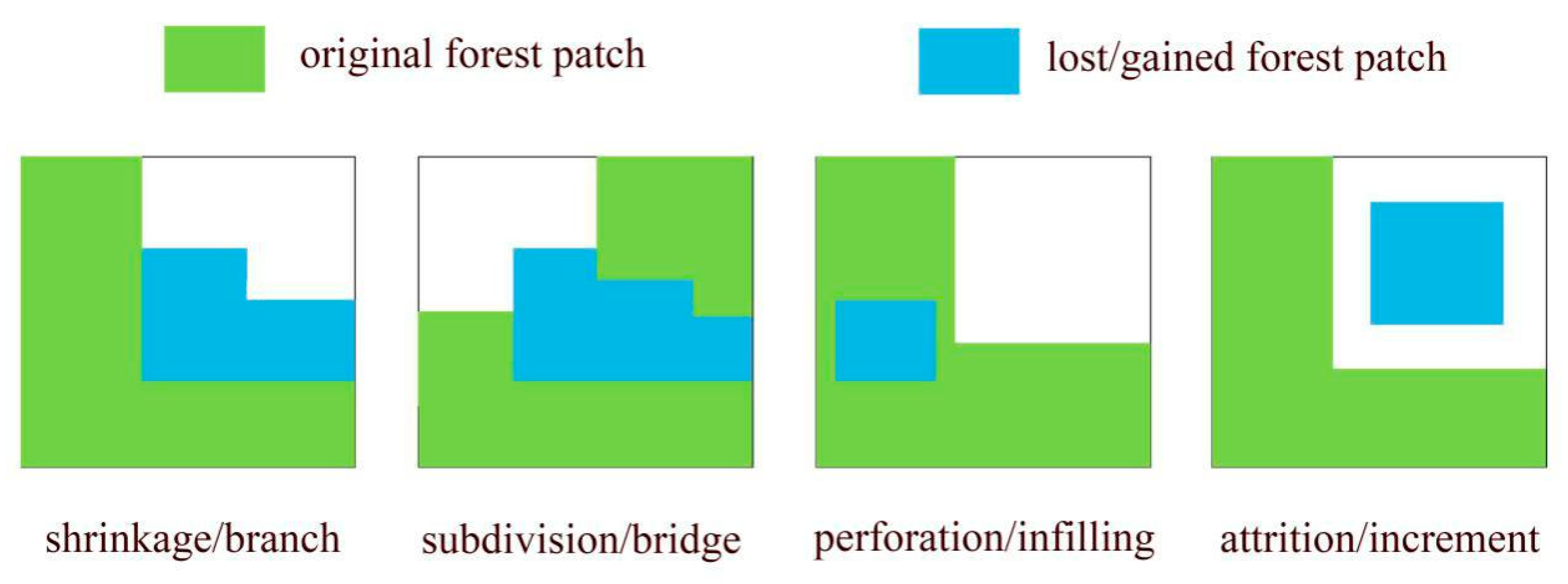
2.3.4. Modelling Forest Spatial Process

Li and Yang [25] divided the forest loss process into perforation, subdivision, shrinkage and attrition components. Ren et al. [26] developed a forest restoration model that classified the forest restoration patches as increment and expansion processes. Based on this model, we divided the forest restoration process into infilling, branch, bridge and increment components. Attrition means that lost forest patches are not connected to any original forest patch (the unchanged patches in both phases). Perforation indicates that lost forest patches are surrounded by original forest patches. Shrinkage implies that one end of a lost patch is connected to an original forest patch, while the other end is connected to a non-forest patch. Subdivision means that lost forest patches are connected to different original forest patches (Figure 3). The four categories of forest restoration processes are similar to those of the forest loss processes. Perforation corresponds to infilling, subdivision corresponds to bridge, shrinkage corresponds to branch and attrition corresponds to the increment component (Figure 3).

Identifying forest loss/recovery process categories was based on the number of unchanged forest patches and non-forest patches around the lost/gained forest patches. Firstly, lost forest pixels, unchanged forest pixels and non-forest pixels were obtained by comparing the bi-temporal forest/non-forest products, where the unchanged forest was set to 1, the non-forest was set to 0 and the lost forest was set to null. Then, we reassigned different values to each unchanged forest patch (starting with the number 1). Next, we calculated the maximum value of each pixel in the lost patches within the 8-pixel neighborhood and assigned this maximum value to the central pixel. Finally, we counted the number of different values in each lost patch. If the lost forest patch contained two different values, then the patch was shrinkage. If the lost forest patch contained three or more different values, then the patch was subdivision. If the lost forest patch contained only one value, and the value was 0, then it experienced attrition, while the remaining patches were perforation patches. The forest restoration process model was similar to the forest loss process model, except that the lost patches were replaced with gained patches.

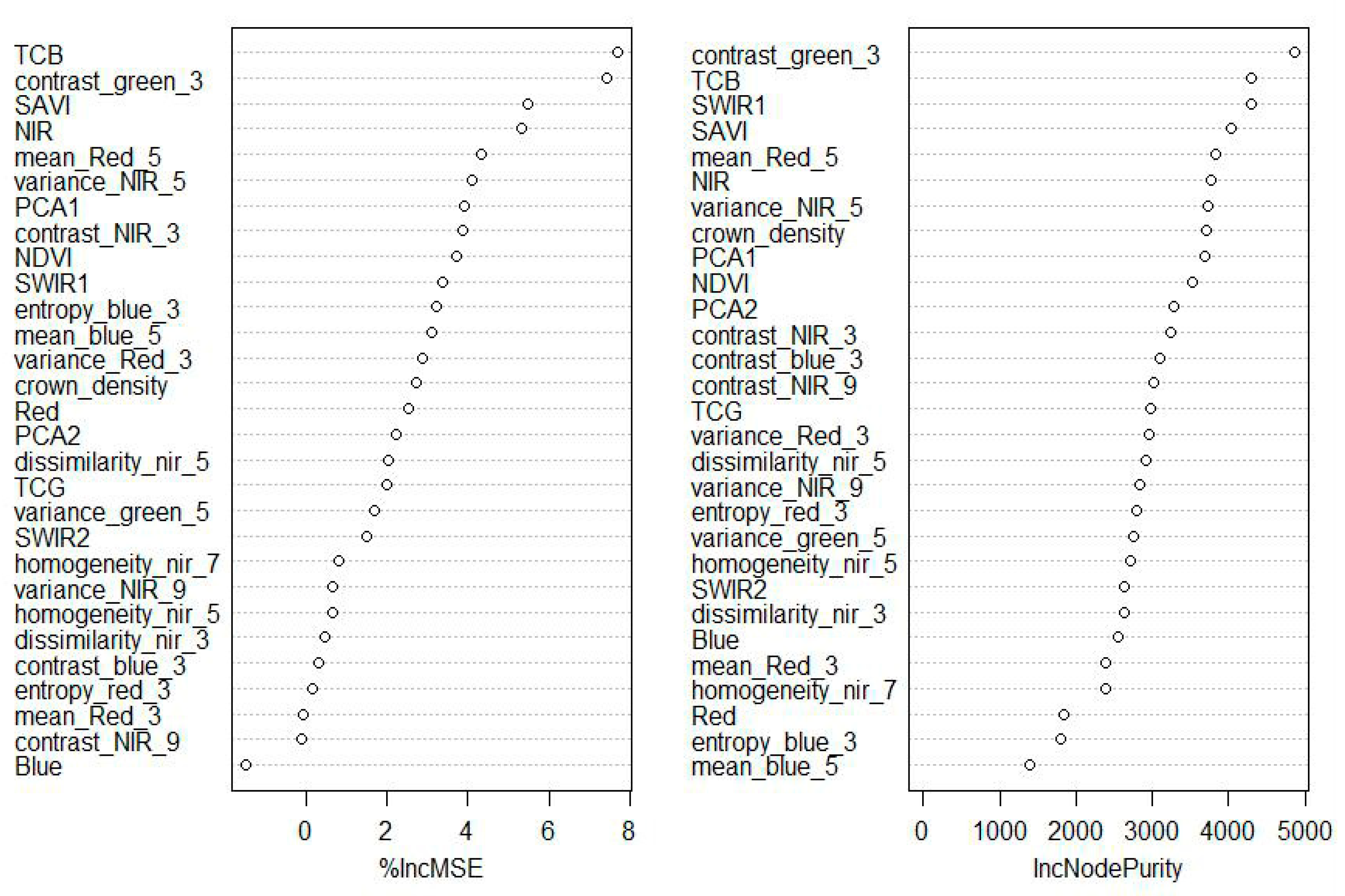
2.3.5. Remote Sensing Predictor Variables for AGB Model

We examined the AGB changes for 2006 and 2017 to determine the impacts of restoration on ecosystem functions. A large number of predictive variables were used for AGB assessment, including six surface reflectance bands of the Landsat images for 2006 and 2017 and other derived variables, including spectral indices, tasseled cap transformation, principal components and texture information. Surface reflectance data were directly derived by USGS. The spectral indices mainly reflect the vegetation differences in the visible red, near-infrared and soil background, and the indices used in this study were the normalized difference vegetation index (NDVI), enhanced vegetation index (EVI) and soil-adjusted vegetation index (SAVI) [43,44,45]. The tasseled cap transformation uses a linear combination of six Landsat bands and specialized coefficient matrices to create a set of new features. The first three features include the most useful information, named brightness, wetness and greenness [46]. Principal component analysis (PCA) is an orthogonal linear transformation of multi-dimensional data, which is completed by diagonalizing the covariance matrix of the original data. Then, PCA can be used for dimensionality reduction by projecting each data point onto only the first few principal components to eliminate redundant information without losing important information, and it attains a closer relationship with AGB than a single spectral band [47,48]. We followed the gray-level co-occurrence matrix approach that uses the gray tone spatial correlation matrix to calculate texture values, including mean, variance, homogeneity, contrast, dissimilarity, entropy, second moment and correlation [49]. The study calculated 8 kinds of remote sensing texture information with 4 different window sizes: 3 × 3, 5 × 5, 7 × 7 and 9 × 9 (

Table 4. The predictor variables for aboveground biomass (AGB) modeling.

Type	Variable	Equation
Surface reflectance	Blue, red, green, near-infrared (NIR), shortwave infrared 1(SWIR1), shortwave infrared 2 (SWIR2)
Spectral Indices	NDVI	(NIR − Red)/(NIR + Red)
	EVI	2.5 × (NIR − Red)/(NIR + 6× Red − 7.5 × Blue + 1)
	SAVI	(1 + 0.5) × (NIR − Red)/(NIR + Red + 0.5)
Tasseled cap transformations	Tasseled cap brightness (TCB), tasseled cap greenness (TCG), tasseled cap wetness (TCW)
Texture analysis	Mean, variance, homogeneity, contrast, dissimilarity, entropy, second moment, correlation
PCA	PCA1, PCA2 (the first and second principal components containing the most image information)

). Last, we extracted the mean value of all the pixels in the corresponding forest stand subcompartment and incorporated the crown density as a predictor.

2.3.6. Random Forest Modeling and Variable Selection

The random forest (RF) algorithm is a flexible machine learning algorithm composed of a large number of decision trees with a high prediction accuracy, low probability of overfitting and good tolerance for outliers [50]. Thus, we used it to identify important predictor variables, simulate the relationship between them and the AGB and finally applied the well-trained model to map the AGB throughout the entire study area. We constructed the AGB model using the RF package of R software. There were 3 parameters to be set in the model (ntree, mtry and nodesize). The ntree parameter is the number of decision trees and 500 trees (ntree) were used for AGB modeling. The mtry parameter is the number of variables to be tested at each node and it was set to 4. The nodesize parameter is the minimum number of decision tree nodes and it was set to the default value of 1 in the current work.

The irrelevant and redundant variables of a model reduce its efficiency [29]. Thus, the importance of all variables was ranked by the percent increase mean square error (PercentIncMSE) and the increase in NodePurity (IncNodePurity) in the function of the feature importance for the RF package. PercentIncMSE is defined as the decrease in accuracy when a given variable was excluded from decision trees. IncNodePurity measures the decrease in node impurities attributable to the splits of a given variable [29]. The higher PercentIncMSE and IncNodePurity are, the more important these variables are [50]. Based on the ranking of both these indicators, we finally selected 14 variables (crown density; NIR; SWIR1; NDVI; SAVI; TCB; TCG; window size of 3×3: contrast_Green, variance_Red and contrast_NIR; window size of 5×5: variance_NIR and mean_Red; PCA1, and PCA2) (Figure 4).

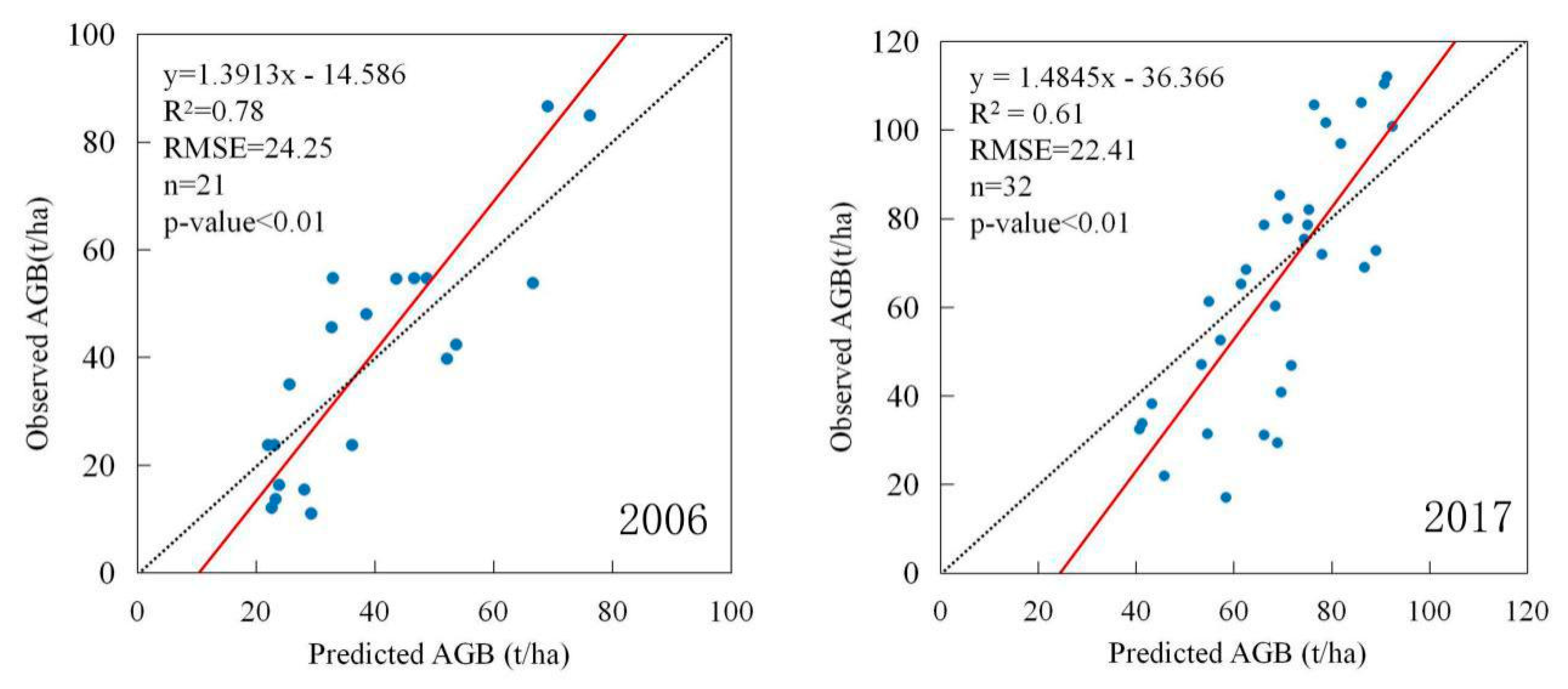
2.3.7. Model Accuracy Assessment and Validation

The performance of the fitted model needs to be evaluated to determine whether the model can reflect the actual situation. After the AGB model was created, the remaining samples were fed to the model to obtain AGB predictions, and we then compared these values to actual observations. The coefficient of determination (R²) and root mean square error (RMSE) were chosen for model evaluation. Generally, the larger R² is and the smaller RMSE is, the better the model prediction capability.

$$R^2=1-\frac{{{\displaystyle \sum }}_{i=1}^n{\left(y_i-{\widehat{y}}_i\right)}^2}{{{\displaystyle \sum }}_{i=1}^n{\left(y_i-\overline{y}\right)}^2}$$

(1)

$$\mathrm{RMSE}=\sqrt{{\displaystyle \sum }_{i=1}^n\frac{{\left(y_i-{\widehat{y}}_i\right)}^2}{n}}$$

(2)

where $y_i$ is the observed AGB, ${\widehat{y}}_i$ is the predicted AGB based on the model, $\overline{y}$ is the mean of all observed AGB and n is the number of samples.

3. Results

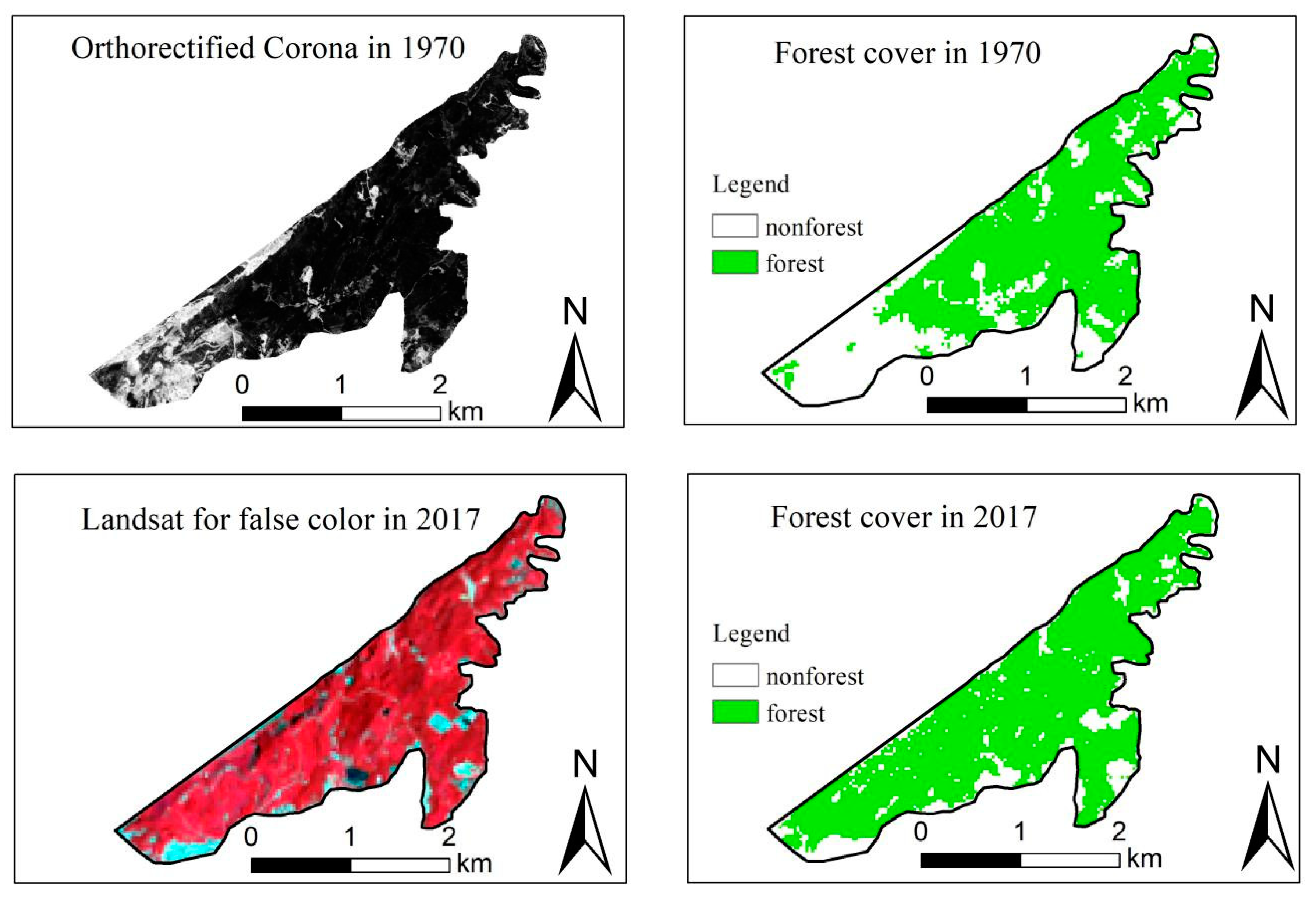
3.1. Accuracy Assessment for Ortho-Rectification and Forest Cover

We generated 11 GCPs on the ortho-rectified Corona image and Landsat to assess the errors of ortho-rectification. The errors of all GCPs were controlled within half a pixel (15 m) (

Table 5. Root mean square error (RMSE) of Corona data ortho-rectification in 1967 and 1970.

Year	Number of GCPs	RMSE x (m)	RMSE y (m)	Total RMSE (m)
1967	11	3.94	2.14	4.70
1970	11	3.76	3.01	4.82

). So, the geographic accuracy of Corona data was comparable to Landsat (Figure 5), and there were few false changes caused by errors in the ortho-rectification (Table 5).

By comparing the forest cover maps for 2006 and 2017 with the inventory data, we found that the overall accuracies of the two-year classification results were above 90%, and the highest overall accuracy was 94.8% in 2006, while the lowest overall accuracy was 93.0% in 2017 (

Table 6. Accuracy assessment of the forest cover maps of 2006 and 2017.

Year	Class	Producer Accuracy (%)	User Accuracy (%)	Overall Accuracy (%)
2006	forest	94.0	98.2	94.8
	non-forest	97.6	84.8
2017	forest	98.1	93.3	93.0
	non-forest	74.4	91.4

). Such accuracies were suitable for characterizing changes in forest cover compared to other literature [10,51].

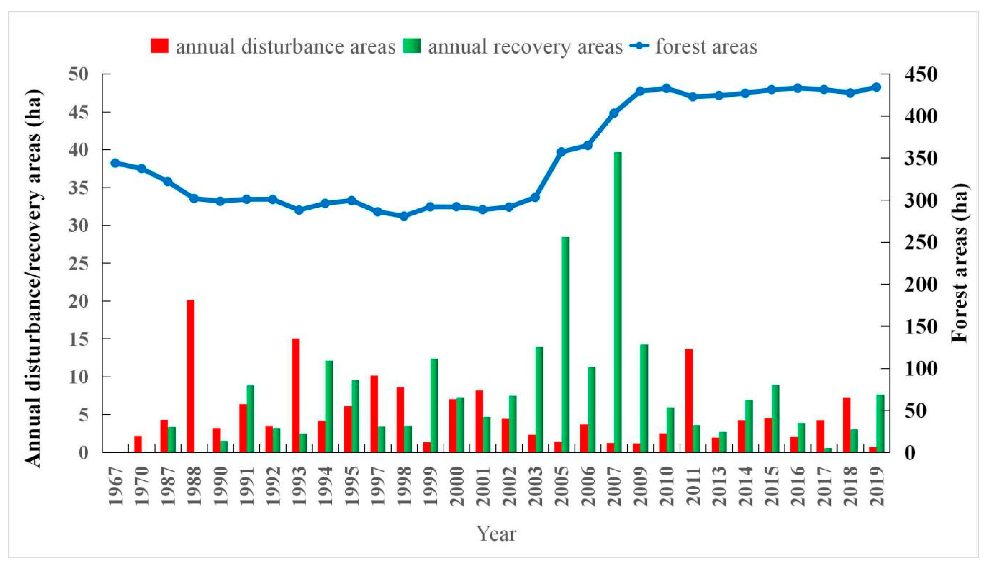
3.2. Spatio-Temporal Dynamics of Forest Cover

By applying visual interpretation and the VCT model to Corona and Landsat, the estimates of changes in forest cover, annual disturbance and recovery were obtained (Figure 6 and Figure 7). The forest cover areas on Mt. Mufu continuously decreased from 343.89 in 1967 to 298.44 ha in 1990, indicating a continuous mining disturbance. Subsequently, the changes in forest cover were less apparent from 1990 to 2003, after which the forest areas markedly increased due to some restoration projects, reaching the maximum areas in 2019 with the forest cover of 434.16 ha (Figure 6). The smallest annual forest disturbance area was 0.72 ha in 2019, whereas the largest disturbance area occurred in 1988, at 20.16 ha. Generally, the disturbance areas before 1999 were larger than those after 1999. There were fewer or no forest restoration areas before 1991, and there were substantial increases in the forest restoration area from 1999 to 2009 (Figure 6). After 2009, the annual forest restoration area was basically maintained between 4 and 8 ha. Over the entire time series, the largest annual restoration area was 39.69 ha, which occurred in 2007, and the smallest annual forest restoration area was 0, occurring in 1970 and 1988 (Figure 6).

A pixel may experience multiple disturbances or recovery during the entire time series analysis, we only recorded the year and location of the first disturbance or recovery. From 1967 to 1990, large forest loss areas occurred in regions (1) and (2), which were also the mining areas (Figure 7). Only sporadic and small forest areas disappeared after 1990, with the exception of the notable forest loss (light green and purple) in the lower right of Mt. Mufu in 1997 and 2017. Forests covered almost the entire mountain in 2019 based on the recovery map (Figure 7). The forest restoration areas from 1970 to 1987 were small and mainly concentrated in the lower and edge parts of the mountain. Medium-scale vegetation restoration was firstly conducted at mining site (1) from 1993 to 1997. Major forest restoration occurred between 2005 and 2009 at mining sites (2) and (3) (Figure 7).

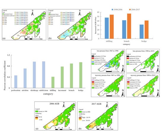
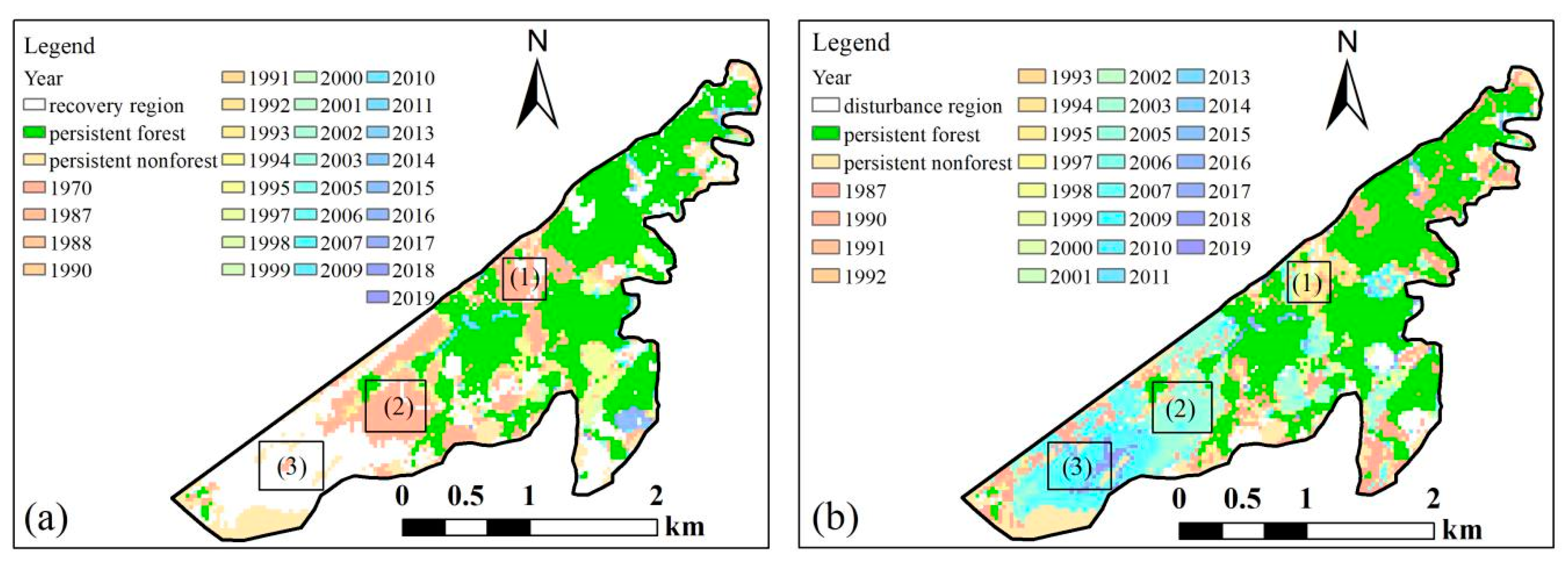
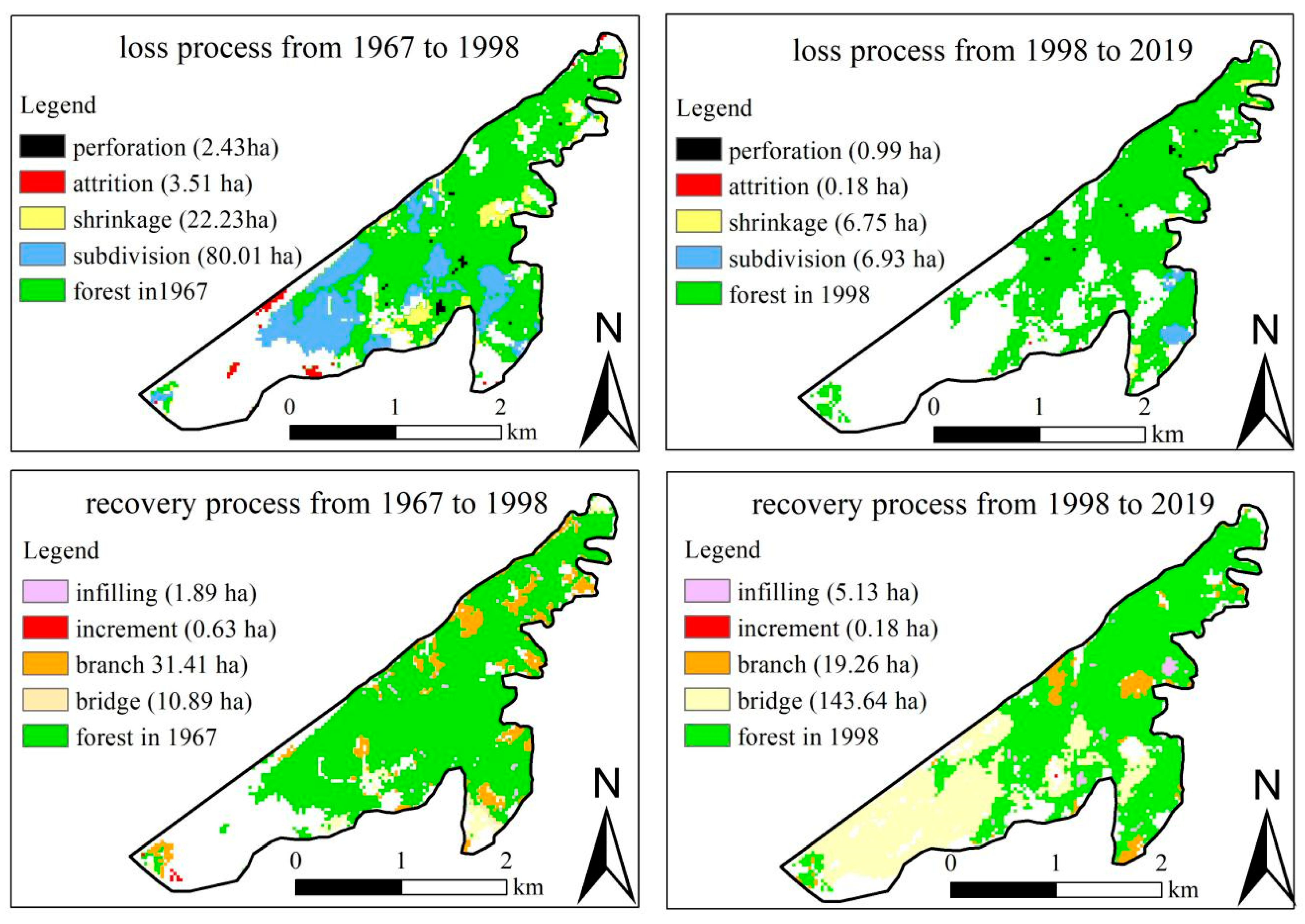
3.3. Analysis of the Spatial Process of Forest Change

3.3.1. Effects of Forest Changes on Landscape Spatial Structure

For the effects of forest changes on the landscape spatial structure, we firstly calculated the area of annual forest loss/recovery and the corresponding area of each category for the spatial process in the adjacent year from 1967 to 2019. We used the Pearson correlation coefficient (r) to express the relationship between annual forest loss (recovery) and each category of the forest loss (recovery) process model. The Pearson correlation coefficient (r) reflects the strength of the linear correlation between two variables. The higher r is, the stronger the correlation is. Perforation, attrition, shrinkage and subdivision (infilling, increment, branch and bridge) all had positive correlations with forest loss (recovery). Subdivision had the strongest correlation with annual forest loss with r = 0.96, and shrinkage ranked second with r = 0.92. The weakest r was between annual forest loss and perforation, only at 0.47. Bridge had the strongest correlation with forest recovery at r = 0.91, while infilling had the lowest correlation with forest restoration, only at r = 0.52 (

Table 7. Pearson correlation coefficient between forest loss (recovery) and each type of the process model (n = 29).

Category	Annual Forest Loss	Category	Annual Forest Recovery
perforation	0.47	infilling	0.52
attrition	0.58	increment	0.79
shrinkage	0.92	branch	0.89
subdivision	0.96	bridge	0.91

Note: coefficient is significant at the 0.01 level.

). These results suggested forest loss or gain greatly changed the structure connectivity of the forest landscape pattern.

3.3.2. Spatio-temporal Changes of Forest Spatial Processes

Since the restoration projects began to be implemented in 1999, we adopted 1998 as a benchmark year to analyze the spatial maps of forest loss and recovery. From 1967 to 1998, large-scale subdivision and shrinkage patches were distributed in the lower left and middle of Mt. Mufu, occupying the areas of 80.01 and 22.23 ha, respectively. The lost forest areas attributed to attrition and perforation were smaller than 4 ha. Attrition was mainly observed in the lower left of Mt. Mufu, while perforation mainly transpired in the middle of the mountain (Figure 8). During the second period, the areas of all types of forest loss processes decreased, with subdivision substantially decreasing to 6.93 ha. Besides, the location of subdivision shifted to the lower right of Mt. Mufu. The areas of the perforation and attrition were even less than 1 ha. During the forest restoration process from 1967 to 1998, the branch area ranked first with an area of 31.41 ha, which mainly distributed in the edge and middle of the mountain. The smallest area of patches was observed for the increment process (Figure 8). During the period from 1998 to 2019, the bridge area sharply increased to 143.64 ha and this process almost filled the forest cover of the entire mountain. Large bridge areas were observed in the lower left of the mountain, and the branch process mainly occurred in the middle of the mountain. The spaces occupied by infilling and increment were relatively small at only 5.13 and 0.18 ha.

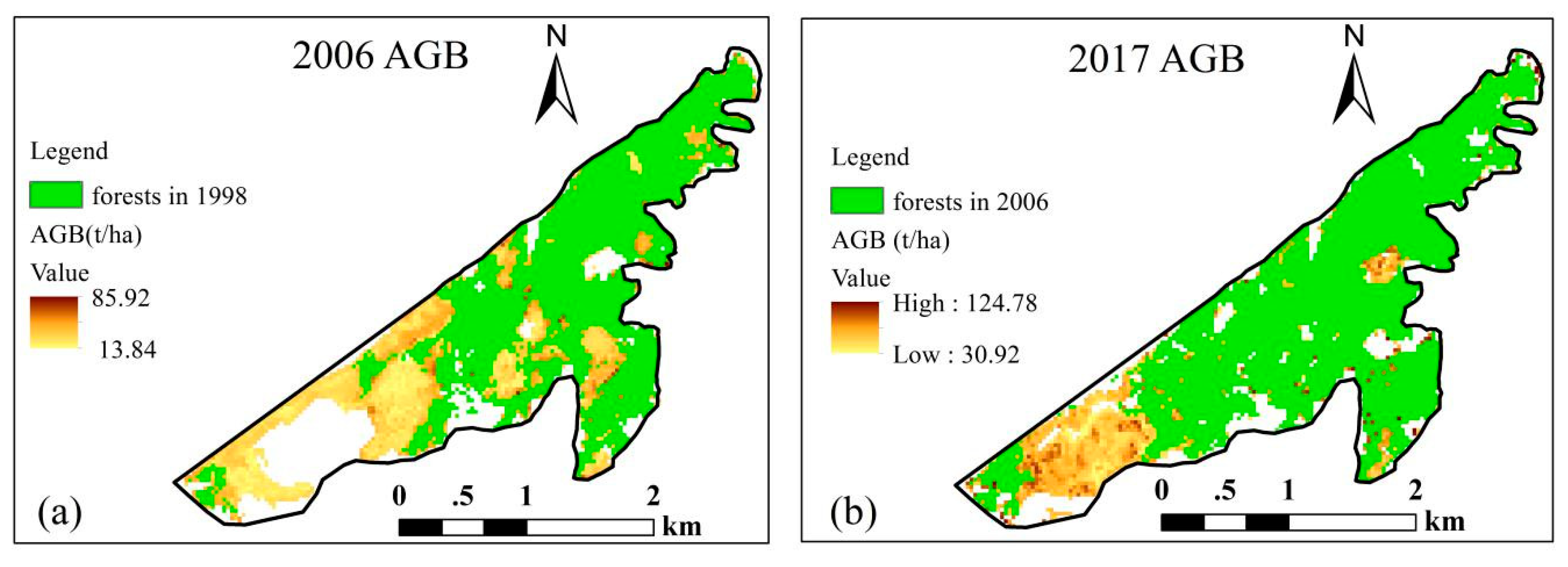
3.4. Evaluation of Ecosystem Function Based on AGB Dynamics

A large increase in forest cover occurred in 2005 (Figure 6). Since we did not obtain field data for 2005, we used the 2006 data as an alternative to analyze the changes in forest AGB on Mt. Mufu between 2006 and 2017 to determine the impacts of ecological restoration on ecosystem function over the past 11 years. We validated the AGB model using the test samples. There were 21 test samples for the 2006 AGB model and 32 test samples for the 2017 AGB model. In 2006, the R² value of the linear fitting between the predicted and observed values was 0.78, and the RMSE was 24.25 t/ha. The R² value for the 2017 validation was 0.61, with an RMSE of 22.41 t/ha (Figure 9). Karlson et al. [30] found that the R² between the observed AGB and predicted AGB was 0.57. Li et al. [28] reported that the best R² and RMSE for their AGB model assessment were 0.41 and 23.07 t/ha. Thus, our model performance was better than the ones in the other reported studies, and the subsequent results were considered reliable.

The area covered by forests in 2006 was 364.77 ha, and the area covered by forests in 2017 was 431.37 ha (Figure 6). The corresponding total forest AGB increased from 20,173.35 in 2006 to 31,035.77 t in 2017. Besides, the maximum AGB increased from 85.92 in 2006 to 124.78 t/ha in 2017, and the lowest AGB in 2006 was 13.84 t/ha, after which it increased to 30.92 t/ha in 2017 (

Table 8. Summary of the predicted biomass for the entire study area in 2006 and 2017.

	Minimum AGB (t/ha)	Maximum AGB (t/ha)	Mean AGB (t/ha)	Total AGB (t)
2006	13.84	85.92	48.38	20,173.35
2017	30.92	124.78	73.4	31,035.77

). In addition, the increased AGB due to afforestation was about 15-30 t/ha from 1998 to 2006, while the increased AGB caused by afforestation in 2006–2017 was approximately 30–50 t/ha (Figure 10). These increased AGB all indicated that the ecosystem function was gradually improved.

For the relationships between restored landscape structure and ecological function, we quantitatively determined the increased AGB caused by each restoration process category. It was worth noting that increment was not included because there was few or no samples of this category in both stages. From 1998 to 2006, the maximum value of increased forest AGB was 47.68 t/ha, which was attributed to infilling (

Table 9. Quantitative analysis between landscape structure and ecological function.

1998–2006	Increased AGB (t/ha)	2006–2017	Increased AGB (t/ha)
infilling (4.86 ha)	47.68	infilling (3.6 ha)	54.25
branch (11.34 ha)	41.69	branch (18.72 ha)	56.78
bridge (76.14 ha)	31.85	bridge (61.29 ha)	41.06

). The largest increase in forest AGB from 2006 to 2017 occurred in branch components, which was 56.78 t/ha (Figure 10 and Table 9). The increased AGB of all categories in the second recovery phase was greater than those in the first recovery phase. However, the bridge component accounted for the highest recovery areas with the values of 76.14 and 61.29 ha in both stages, but the corresponding forest AGB was the least and they were less than 42 t/ha (Table 9), indicating that although the connectivity of the landscape structure has increased, there is still much room for improvement in ecological functions.

4. Discussion

4.1. Value and Suitability of Integrating Corona and Landsat Data

The large-scale forest disturbance in Mt. Mufu was mainly attributed to mining activities that occurred in the 1960s [52]. At that time, there were nine quarries and four garbage dumps, of which the largest quarry of “Baiyun” experienced three large-scale expansions from 1965 to 1995. Later, Nanjing government officially started to implement comprehensive management strategies in Mt. Mufu. As a result, eight mines were closed in 1999 [53]. In 2003, the "Baiyun” quarry was fully terminated and accelerated the recovery process. By 2009, 10 artificial greening projects and 2 special ecological restoration projects had been implemented and the forest coverage increased substantially [52].

Based on the above information, we need to rely on remote sensing to obtain more detailed spatial and temporal changes. Vegetation loss and restoration in mining areas often lasts for decades; thus, Landsat has been widely applied in forest change detection due to its ability to cover large scales and its high acquisition time frequency [11,12,54]. However, the processing efficiency and precision assurance of remote sensing images have become some of the challenges of vegetation monitoring [55]. If automated algorithms can be used, this tedious task will be greatly simplified. Regarding fully automated algorithms, LandTrendr is mostly used for vegetation restoration research in mining areas. Dlamini and Xulu [51] studied the value of mine restoration based on the LandTrendr algorithm and produced disturbance and recovery maps of mining areas. In addition, Yang et al. [10] examined the overall accuracies of the estimated mining disturbance and recovery, which were 85.21% and 86.59%, respectively, for LandTrendr. Shen et al. [56] compared the VCT and LandTrendr algorithms and found that both algorithms obtained similar accuracies. The overall VCT accuracy was 78%, and the overall LandTrendr accuracy was 77%. Although VCT and LandTrendr can produce similar accuracy results in disturbance mapping, these methods are performed in different ways and for different purposes. The VCT algorithm detects abrupt forest disturbances such as from fire and logging by detecting deviations of the vegetation index in the time series. The LandTrendr algorithm relies on the spectral segmentation method to detect abrupt disturbance events across all land areas and slower long-term changes. Thus, forest coverage maps need to be included to eliminate disturbance effects from non-forest areas in LandTrendr applications [56,57]. In contrast to previous studies that applied LandTrendr in mine recovery assessment, our study attempted to use the VCT algorithm to directly determine the forest disturbance and restoration map and derived forest cover. The results of the current work showed that the overall accuracy of forest cover mapping in 2006 was 94.8%, and the overall accuracy in 2017 was 93% (Table 6). Such accuracy was considered reliable for long-term change monitoring. In addition to the detection of forest changes in small mining areas, VCT is also suitable for forest changes monitoring at large scales. Zhao et al. [58] used VCT and support vector machine to identify forest disturbance types in the Greater Yellowstone Ecosystem, including wildfire, harvest and other disturbance types. Diao et al. [54] integrated the VCT algorithm and spatial analysis to characterize the disturbed forests in southeastern China from 1987 to 2017. Zhang et al. [41] combined the VCT and the urban impervious surface index to describe the forest loss due to urban expansion in Nanjing. These studies indicated that VCT is not only suitable for mining disturbance monitoring, but also it is appropriate for forest changes caused by other abrupt forest disturbance events.

However, Landsat could not trace the history of forest changes in the 1960s. Declassification of the Corona data in 1995 made it possible to study land cover change beginning in the 1960s due to the high spatial resolution [23]. In this study, our analysis of the forest changes on Mt. Mufu was portrayed from 1967 to 2019, and the results showed that the forest area sharply decreased from 1967–1990. After 2003, the forest area began to increase substantially. Clearly, data-oriented forest information based on Corona and Landsat provided us with a clear picture of how the forest changed when historical forest change documentation was absent. This information can teach us lessons from the disorderly exploitation of natural resources in the past and can improve urban forest management plans to achieve sustainable development in the near future. For example, mining can be terminated, and vegetation remediation can be implemented immediately in mining areas to improve urban landscape esthetics. These actions are highly dependent on available forest change histories. Besides, Corona is also applicable to other regions to reveal the forest change histories in the 1960s. Song et al. [22] proposed an automated classification algorithm based on Corona to extract forest cover information in the eastern United States and central Brazil, which makes it possible to apply Corona to large-scale forests. Nita et al. [59] used the same method of visual interpretation to study forest cutting in Romania after World War II. These examples fully proved Corona’s ability to allow for the reliable identification of spatially explicit forest in other regions. At the same time, these forest cover products can lay the foundation for subsequent landscape structure and ecological function evaluation.

4.2. Assessments and Application of the Landscape Structure and Ecological Function

Although landscape ecology methods have been adopted to measure the forest landscape changes in mining areas, they are usually applicable at specific points [3,16]. Considering that the process of forest landscapes can help us better investigate the relationship between forest changes and landscape structure [25], we adopted two process models. The occurrence of subdivision implied a decrease in connectivity between two forest patches, and shrinkage indicated communication inhibition between forest and non-forest patches. Perforation led to an increase in internal edges, often accompanied by edge effects. Our results showed that subdivision dominated the forest loss process with the area of 80.01 ha and shrinkage ranked second from 1967 to 1998 (Figure 8). Besides, subdivision had the strongest correlation with forest loss (r = 0.96) (Table 7), indicating forest loss reduced the structure connectivity. This derived information is essential for natural resource managers or conservation communities to carry out corresponding recovery actions to eliminate these negative effects. In addition, our work enriched the previous restoration process model and the improved model better evaluated the impact of forest restoration on the landscape structure. For example, there was an increase of 143.64 ha in bridge areas in 1998–2019 and it had a high correlation (r = 0.91) with forest recovery (Figure 8 and Table 7). These results indicated the increased forest cover mainly compensated for the lack of connectivity between the forest areas on Mt. Mufu. However, the higher correlation between increment and forest restoration should not be underestimated. In fact, small and isolated forest areas (increment patches) often suffer from a higher risk of disappearing in the future. Infilling resulted in a more complete forest and promoted the stability of the forest structure. Thus, we concluded that the overall landscape structure layout of the restoration projects was reasonable and forest managers attached great importance to the connection of different forest patches, but they should avoid the occurrence of isolated forests in the future. Lastly, the process model is very practical, and it can be applied to any land cover type as long as the land cover increase or decrease in two phases is obtained.

In addition to the evaluation of the landscape structure, ecological function assessment is also very important. Wang et al. [52] evaluated the state of the Mt. Mufu ecosystem in 2009 and concluded that Mt. Mufu was still in the initial stage of ecological restoration. Pan et al. [60] compared the ecological services values in the early and late stages of ecological restoration on Mt. Mufu and found that the recovery effect in the later period was greater than that in the early period, which was similar to our results. We examined the forest AGB changes in 2006 and 2017 to evaluate the effectiveness of restoration projects. The total AGB in 2006 was smaller than that in 2017, indicating that the progress of late ecological restoration was greater than that of early restoration. However, we also found that the increased AGB was only 30-40 t/ha in most restored forest areas (bridge components), suggesting that the restored ecological function was still low even if the structural connectivity was enhanced. These bridge components mainly occurred in the southwest of the mountain, where the main mining sites were located at that time. Due to the years of mining, there were steep cliffs in the southwest and the soil erosion was extremely serious, which made ecological restoration projects difficult. The increased forest AGB for remaining categories were higher because these elements occurred in the northeast and middle of the mountain (Figure 8 and Figure 10). The ecological environment in these regions was excellent, so the ecological function was also high. In the future, while improving the connectivity of the landscape structure, environmental managers should continue to pay more attention to ecological restoration in the southwest of the mountain and improve the ecological function of plantation forests. Additionally, quantifying the impacts of forest restoration on ecological functions through the dynamics of AGB cannot be only limited to mining areas. Currently, Landsat images coupling field survey data have become the most popular method for evaluating AGB [28,29], so the current evaluation methods are also transferrable to other regions.

4.3. Research Limitations and Future Work

This study provided high-precision forest cover products with long time spans. However, meeting the needs of long-term analysis comes at the expense of the ability to capture subtle changes. In addition, field-based AGB estimation may contain sampling measurement errors, which can lead to errors in the results. Future research should incorporate high-resolution images or LIDAR data to improve the accuracy of forest cover and biomass estimation. Finally, the current work adopted only two years of AGB dynamics to evaluate the effect of ecological restoration, and more evaluation indices should be collected for recovery assessment.

5. Conclusions

This study aims to characterize the spatial and temporal dynamics of forests in specific mining areas, to describe the spatial process of forest landscapes, and to evaluate the AGB changes. The forest cover dramatically decreased due to mining disturbances from 1967 to 1990, and after 2003, the forest cover significantly increased and reached its maximum areas in 2019. The main locations of forest loss and restoration were the former mining sites. The subdivision processes affected larger areas than the remaining three categories in the forest loss process. In the process of forest restoration, the bridge process occupied the main areas and it had a strong correlation with forest restoration (r = 0.91). These indicated that forest loss and restoration changed the structural connectivity of the forests. The forest AGB in 2017 was higher than that in 2006, but the increased AGB in most recovery areas was only 30–40 t/ha, indicating that the ecological restoration of Mt. Mufu still requires greater improvements in the future. All the results revealed past forest changes (coverage, landscape pattern and ecological restoration effects) from a historical perspective, which can help researchers and managers better understand the process of vegetation changes and the effects of restoration projects over time, thereby they can propose more reasonable strategies in the future.

References

1. Bian, Z.; Lei, S.; Inyang, H.I.; Chang, L.; Zhang, R.; Zhou, C.; He, X. Integrated method of RS and GPR for monitoring the changes in the soil moisture and groundwater environment due to underground coal mining. Environ. Geol. 2009, 57, 131–142. [Google Scholar] [CrossRef]
2. Linke, J.; McDermid, G.J. Monitoring landscape change in multi-use west-central Alberta, Canada using the disturbance-inventory framework. Remote Sens. Environ. 2012, 125, 112–124. [Google Scholar] [CrossRef]
3. Zhang, J.; Rao, Y.; Geng, Y.; Fu, M.; Prishchepov, A.V. A novel understanding of land use characteristics caused by mining activities: A case study of Wu’an, China. Ecol. Eng. 2017, 99, 54–69. [Google Scholar] [CrossRef]
4. Hodge, R.A. Mining company performance and community conflict: Moving beyond a seeming paradox. J. Clean. Prod. 2014, 84, 27–33. [Google Scholar] [CrossRef]
5. Jozefowska, A.; Pietrzykowski, M.; Wos, B.; Cajthaml, T.; Frouz, J. The effects of tree species and substrate on carbon sequestration and chemical and biological properties in reforested post-mining soils. Geoderma 2017, 292, 9–16. [Google Scholar] [CrossRef]
6. Lei, S.; Ren, L.; Bian, Z. Time-space characterization of vegetation in a semiarid mining area using empirical orthogonal function decomposition of MODIS NDVI time series. Environ. Earth Sci. 2016, 75, 516. [Google Scholar] [CrossRef]
7. Wang, W.; Hao, W.; Sian, Z.; Lei, S.; Wang, X.; Sang, S.; Xu, S. Effect of coal mining activities on the environment of Tetraena mongolica in Wuhai, Inner Mongolia, China-A geochemical perspective. Int. J. Coal Geol. 2014, 132, 94–102. [Google Scholar] [CrossRef]
8. Laurence, D. Establishing a sustainable mining operation: An overview. J. Clean. Prod. 2011, 19, 278–284. [Google Scholar] [CrossRef]
9. Vintro, C.; Sanmiquel, L.; Freijo, M. Environmental sustainability in the mining sector: Evidence from Catalan companies. J. Clean. Prod. 2014, 84, 155–163. [Google Scholar] [CrossRef] [Green Version]
10. Yang, Y.; Erskine, P.D.; Lechner, A.M.; Mulligan, D.; Zhang, S.; Wang, Z. Detecting the dynamics of vegetation disturbance and recovery in surface mining area via Landsat imagery and LandTrendr algorithm. J. Clean. Prod. 2018, 178, 353–362. [Google Scholar] [CrossRef]
11. Bao, N.; Lechner, A.; Fletcher, A.; Erskine, P.; Mulligan, D.; Bai, Z. SPOTing long-term changes in vegetation over short-term variability. Int. J. Min. Reclam. Environ. 2014, 28, 2–24. [Google Scholar] [CrossRef]
12. Huang, C.; Coward, S.N.; Masek, J.G.; Thomas, N.; Zhu, Z.; Vogelmann, J.E. An automated approach for reconstructing recent forest disturbance history using dense Landsat time series stacks. Remote Sens. Environ. 2010, 114, 183–198. [Google Scholar] [CrossRef]
13. Kennedy, R.E.; Cohen, W.B.; Schroeder, T.A. Trajectory-based change detection for automated characterization of forest disturbance dynamics. Remote Sens. Environ. 2007, 110, 370–386. [Google Scholar] [CrossRef]
14. Sonter, L.J.; Moran, C.J.; Barrett, D.J.; Soares, B.S. Processes of land use change in mining regions. J. Clean. Prod. 2014, 84, 494–501. [Google Scholar] [CrossRef] [Green Version]
15. Ma, Q.; He, C.; Fang, X. A rapid method for quantifying landscape-scale vegetation disturbances by surface coal mining in arid and semiarid regions. Landsc. Ecol. 2018, 33, 2061–2070. [Google Scholar] [CrossRef]
16. Wang, S.; Huang, J.; Yu, H.; Ji, C. Recognition of Landscape Key Areas in a Coal Mine Area of a Semi-Arid Steppe in China: A Case Study of Yimin Open-Pit Coal Mine. Sustainability 2020, 12, 2239. [Google Scholar] [CrossRef] [Green Version]
17. Wu, Q.; Pang, J.; Qi, S.; Li, Y.; Han, C.; Liu, T.; Huang, L. Impacts of coal mining subsidence on the surface landscape in Longkou city, Shandong Province of China. Environ. Earth Sci. 2009, 59, 783–791. [Google Scholar] [CrossRef]
18. De Simoni, B.S.; Praca Leite, M.G. Assessment of rehabilitation projects results of a gold mine area using landscape function analysis. Appl. Geogr. 2019, 108, 22–29. [Google Scholar] [CrossRef]
19. Wang, Z.; Lechner, A.M.; Yang, Y.; Baumgartl, T.; Wu, J. Mapping the cumulative impacts of long-term mining disturbance and progressive rehabilitation on ecosystem services. Sci. Total Environ. 2020, 717. [Google Scholar] [CrossRef]
20. Zibret, G.; Gosar, M.; Miler, M.; Alijagic, J. Impacts of mining and smelting activities on environment and landscape degradation-Slovenian case studies. Land Degrad. Dev. 2018, 29, 4457–4470. [Google Scholar] [CrossRef] [Green Version]
21. Huang, C.; Kim, S.; Song, K.; Townshend, J.R.G.; Davis, P.; Altstatt, A.; Rodas, O.; Yanosky, A.; Clay, R.; Tucker, C.J.; et al. Assessment of Paraguay’s forest cover change using Landsat observations. Glob. Planet. Chang. 2009, 67, 1–12. [Google Scholar] [CrossRef]
22. Song, D.-X.; Huang, C.; Sexton, J.O.; Channan, S.; Feng, M.; Townshend, J.R. Use of Landsat and Corona data for mapping forest cover change from the mid-1960s to 2000s: Case studies from the Eastern United States and Central Brazil. ISPRS J. Photogramm. Remote Sens. 2015, 103, 81–92. [Google Scholar] [CrossRef] [Green Version]
23. McDonald, R.A. Corona: Success for space reconnaissance, a look into the Cold War, and a revolution in intelligence. Photogramm. Eng. Remote Sens. 1995, 61, 689–720. [Google Scholar]
24. Narama, C.; Kaab, A.; Duishonakunov, M.; Abdrakhmatov, K. Spatial variability of recent glacier area changes in the Tien Shan Mountains, Central Asia, using Corona (similar to 1970), Landsat (similar to 2000); ALOS (similar to 2007) satellite data. Glob. Planet. Chang. 2010, 71, 42–54. [Google Scholar] [CrossRef]
25. Li, S.; Yang, B. Introducing a new method for assessing spatially explicit processes of landscape fragmentation. Ecol. Indic. 2015, 56, 116–124. [Google Scholar] [CrossRef]
26. Ren, X.; Lv, Y.; Li, M. Evaluating, differences in forest fragmentation and restoration between western natural forests and southeastern plantation forests in the United States. J. Environ. Manag. 2017, 188, 268–277. [Google Scholar] [CrossRef]
27. Badreldin, N.; Sanchez-Azofeifa, A. Estimating Forest Biomass Dynamics by Integrating Multi-Temporal Landsat Satellite Images with Ground and Airborne LiDAR Data in the Coal Valley Mine, Alberta, Canada. Remote Sens. 2015, 7, 2832–2849. [Google Scholar] [CrossRef] [Green Version]
28. Li, C.; Li, Y.; Li, M. Improving Forest Aboveground Biomass (AGB) Estimation by Incorporating Crown Density and Using Landsat 8 OLI Images of a Subtropical Forest in Western Hunan in Central China. Forests 2019, 10, 104. [Google Scholar] [CrossRef] [Green Version]
29. Shen, W.; Li, M.; Huang, C.; Wei, A. Quantifying Live Aboveground Biomass and Forest Disturbance of Mountainous Natural and Plantation Forests in Northern Guangdong, China, Based on Multi-Temporal Landsat, PALSAR and Field Plot Data. Remote Sens. 2016, 8, 595. [Google Scholar] [CrossRef] [Green Version]
30. Karlson, M.; Ostwald, M.; Reese, H.; Sanou, J.; Tankoano, B.; Mattsson, E. Mapping Tree Canopy Cover and Aboveground Biomass in Sudano-Sahelian Woodlands Using Landsat 8 and Random Forest. Remote Sens. 2015, 7, 10017–10041. [Google Scholar] [CrossRef] [Green Version]
31. Li, L.; Tang, G.G.; Xu, X.G. Studies on Flora of Mountain Mufu Nanjing. J. Nanjing For. Univ. 2006, 30, 38–42. (In Chinese) [Google Scholar]
32. Li, M.; Huang, C.; Shen, W.; Ren, X.; Lv, Y.; Wang, J.; Zhu, Z. Characterizing long-term forest disturbance history and its drivers in the Ning-Zhen Mountains, Jiangsu Province of eastern China using yearly Landsat observations (1987–2011). J. For. Res. 2016, 27, 1329–1341. [Google Scholar] [CrossRef]
33. Zhao, Q.; Ding, D.S.; Yan, C.H. Landscape Ecological Assessment and Planning of Mu-Yan Scenic Spot, Nanjing. Entia Geogr. Sin. 2005, 25, 113–118. (In Chinese) [Google Scholar]
34. Altmaier, A.; Kany, C. Digital surface model generation from CORONA satellite images. ISPRS J. Photogramm. Remote Sens. 2002, 56, 221–235. [Google Scholar] [CrossRef]
35. Galiatsatos, N. The Shift from Film to Digital Product: Focus on CORONA Imagery. Photogramm. Fernerkund. Geoinf. 2009, 251–260. [Google Scholar] [CrossRef] [Green Version]
36. Xie, X.; Wang, Q.; Dai, L.; Su, D.; Wang, X.; Qi, G.; Ye, Y. Application of China’s National Forest Continuous Inventory Database. Environ. Manag. 2011, 48, 1095–1106. [Google Scholar] [CrossRef]
37. Lei, X.D.; Tang, M.P.; Lu, Y.C.; Hong, L.X.; Tian, D.L. Forest inventory in China: Status and challenges. Int. For. Rev. 2009, 11, 52–63. [Google Scholar] [CrossRef]
38. Fang, J.Y.; Chen, A.P.; Peng, C.H.; Zhao, S.Q.; Ci, L. Changes in forest biomass carbon storage in China between 1949 and 1998. Science 2001, 292, 2320–2322. [Google Scholar] [CrossRef]
39. Zeng, W.-S. Research on Forest Biomass and Productivity in Yunnan. Contral South For. Inventory Plan. 2005, 4, 1–3. (In Chinese) [Google Scholar]
40. Tappan, G.G.; Hadj, A.; Wood, E.C.; Lietzow, R.W. Use of Argon, Corona; Landsat Imagery to Assess 30 Years of Land Resource Changes in West-Central Senegal. Photogramm. Eng. Remote Sens. 2000, 66, 727–736. [Google Scholar]
41. Zhang, Y.; Shen, W.; Li, M.; Lv, Y. Assessing spatio-Temporal Changes in forest cover and fragmentation under urban expansion in Nanjing, eastern China, from long-term Landsat observations (1987–2017). Appl. Geogr. 2020, 117. [Google Scholar] [CrossRef]
42. Foody, G.M. Status of land cover classification accuracy assessment. Remote Sens. Environ. 2002, 80, 185–201. [Google Scholar] [CrossRef]
43. Rouse, J.; Hass, R.H.; Schell, J.A.; Deering, D. Monitoring Vegetation Systems in the Great Plains with ERTS; NASA Special Publication: Washington, DC, USA, 1973.
44. Huete, A.; Didan, K.; Miura, T.; Rodriguez, E.P.; Gao, X.; Ferreira, L.G. Overview of the radiometric and biophysical performance of the MODIS vegetation indices. Remote Sens. Environ. 2002, 83, 195–213. [Google Scholar] [CrossRef]
45. Huete, A.R. A soil-adjusted vegetation index (SAVI). Remote Sens. Environ. 1988, 25, 295–309. [Google Scholar] [CrossRef]
46. Crist, E.P.; Cicone, R.C. A Physically-Based Transformation of Thematic Mapper Data—The TM Tasseled Cap. IEEE Trans. Geosci. Remote Sens. 1984, 3, 256–263. [Google Scholar] [CrossRef]
47. Byrne, G.F.; Crapper, P.F.; Mayo, K.K. Monitoring land-cover change by principal component analysis of multitemporal landsat data. Remote Sens. Environ. 1980, 10, 175–184. [Google Scholar] [CrossRef]
48. Lu, D.; Chen, Q.; Wang, G.; Liu, L.; Li, G.; Moran, E. A survey of remote sensing-based aboveground biomass estimation methods in forest ecosystems. Int. J. Digit. Earth 2016, 9, 63–105. [Google Scholar] [CrossRef]
49. Haralick, R.M.; Shanmugam, K.; Dinstein, I. Textural Features for Image Classification. IEEE Trans. Syst. Man Cybern. 1973, SMC3, 610–621. [Google Scholar] [CrossRef] [Green Version]
50. Breiman, L. Random forests. Mach. Learn. 2001, 45, 5–32. [Google Scholar] [CrossRef] [Green Version]
51. Dlamini, L.Z.D.; Xulu, S. Monitoring Mining Disturbance and Restoration over RBM Site in South Africa Using LandTrendr Algorithm and Landsat Data. Sustainability 2019, 11, 6916. [Google Scholar] [CrossRef] [Green Version]
52. Wang, J.; Li, Z.; Hu, X.; Wang, J.; Wang, D.; Qin, P. The ecological potential of a restored abandoned quarry ecosystem in Mt. Mufu, Nanjing, China. Ecol. Eng. 2011, 37, 833–841. [Google Scholar] [CrossRef]
53. Liu, G.H.; Shu, H.L.; Zhang, J.C. Niche of Broussonetia papyrifera Population and Main Associated Species Naturally Revegetabled in Mine Spoil Nanjing Mufu Mountains. Res. Soil Water Conserv. 2007, 14, 184–185. (In Chinese) [Google Scholar]
54. Diao, J.; Feng, T.; Li, M.; Zhu, Z.; Liu, J.; Biging, G.; Zheng, G.; Shen, W.; Wang, H.; Wang, J.; et al. Use of vegetation change tracker, spatial analysis; random forest regression to assess the evolution of plantation stand age in Southeast China. Ann. For. Sci. 2020, 77, 27. [Google Scholar] [CrossRef]
55. Masek, J.G.; Hayes, D.J.; Hughes, M.J.; Healey, S.P.; Turner, D.P. The role of remote sensing in process-scaling studies of managed forest ecosystems. For. Ecol. Manag. 2015, 355, 109–123. [Google Scholar] [CrossRef] [Green Version]
56. Shen, W.; Li, M.; Wei, A. Spatio-temporal variations in plantation forests’ disturbance and recovery of northern Guangdong Province using yearly Landsat time series observations (1986–2015). Chin. Geogr. Sci. 2017, 27, 600–613. [Google Scholar] [CrossRef]
57. Schroeder, T.A.; Moisen, G.G.; Healey, S.P.; Cohen, W.B. Adding value to the FIA inventory: Combining FIA data and satellite observations to estimate forest disturbance. In Moving from Status to Trends: Forest Inventory and Analysis (FIA) Symposium 2012; Department of Agriculture, Forest Service, Northern Research Station: Newtown Square, PA, USA, 2012. [Google Scholar]
58. Zhao, F.; Huang, C.Q.; Zhu, Z.L. Use of Vegetation Change Tracker and Support Vector Machine to Map Disturbance Types in Greater Yellowstone Ecosystems in a 1984–2010 Landsat Time Series. IEEE Geosci. Remote Sens. Lett. 2015, 12, 1650–1654. [Google Scholar] [CrossRef]
59. Nita, M.D.; Munteanu, C.; Gutman, G.; Abrudan, I.V.; Radeloff, V.C. Widespread forest cutting in the aftermath of World War II captured by broad-scale historical Corona spy satellite photography. Remote Sens. Environ. 2018, 204, 322–332. [Google Scholar] [CrossRef]
60. Pan, Y.; Wang, L.C.; Zhang, Y. Assessment of restoration effects of abandoned mininglands in mufushan mountain based on ecosystem value. Res. Soil Water Conserv. 2019, 26, 180–186. (In Chinese) [Google Scholar]
Figure 1. Spatial location of Mt. Mufu in Nanjing City, Jiangsu Province, China (ac); the true color composite of Mt. Mufu in 2009 (Band_3: red, Band_2: green, Band_1: blue), and the spatial distribution of field plots in 2006 and 2017 (d).
Remotesensing 12 03191 g001
Figure 2. Workflow diagram of the current analysis.
Remotesensing 12 03191 g002
Figure 3. Schematic diagram of forest loss and restoration process analysis.
Remotesensing 12 03191 g003
Figure 4. Importance of predictor variables.
Remotesensing 12 03191 g004
Figure 5. Ortho-rectified Corona, Landsat false color composite and derived forest cover distribution maps in 1970 and 2017.
Remotesensing 12 03191 g005
Figure 6. Changes in the forest cover, annual disturbance and annual recovery on Mt. Mufu from visual interpretation and the VCT model applied to the integrated Corona and Landsat data.
Remotesensing 12 03191 g006
Figure 7. Forest loss and recovery maps: (a) first forest loss and (b) first forest recovery; (1), (2) and (3) indicate the former mining regions.
Remotesensing 12 03191 g007
Figure 8. Spatial process map of forest loss and restoration.
Remotesensing 12 03191 g008
Figure 9. Relationship between the predicted and observed AGB values for the test samples with the random forest model.
Remotesensing 12 03191 g009
Figure 10. AGB evaluation in (a) 2006 and (b) 2017.
Remotesensing 12 03191 g010