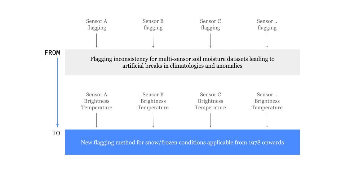
Reconciling Flagging Strategies for Multi-Sensor Satellite Soil Moisture Climate Data Records

 ,
,  ,
,  ,
,
Abstract
:
1. Introduction
- A critical flag is used by the dataset producer to decide that the retrieved SM value is not considered appropriate for dissemination and hence is replaced by Not a Number (NaN). Therefore, well-performing critical flags lead to a reduction of data availability and an improvement of the data quality;
- An advisory flag indicates that the data value should be interpreted carefully and can be filtered out by the user.
2. Data
2.1. Data
2.1.1. Satellite Data
AMSR2 Tb Sensor Data Products
The SMOS SM Sensor Data Products
The SMAP SM Sensor Data Products
The ESA CCI SM Multi-Sensor Data Products
2.1.2. Ground Observations
2.2. Flagging Algorithms
2.2.1. ESA CCI SM Flags
2.2.2. SMOS SM Flags
2.2.3. SMAP SM Flags
3. Methods
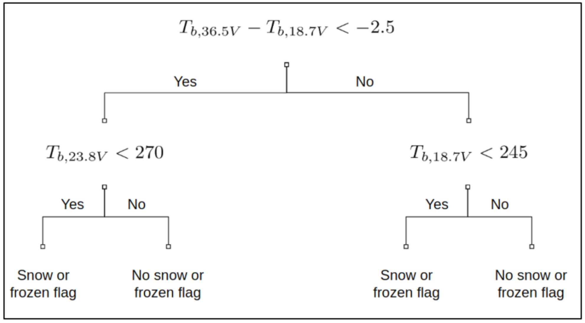
3.1. A New Flagging Strategy for Snow and Ice
3.2. Flagging Evaluation Approach
3.2.1. Flagging Differences
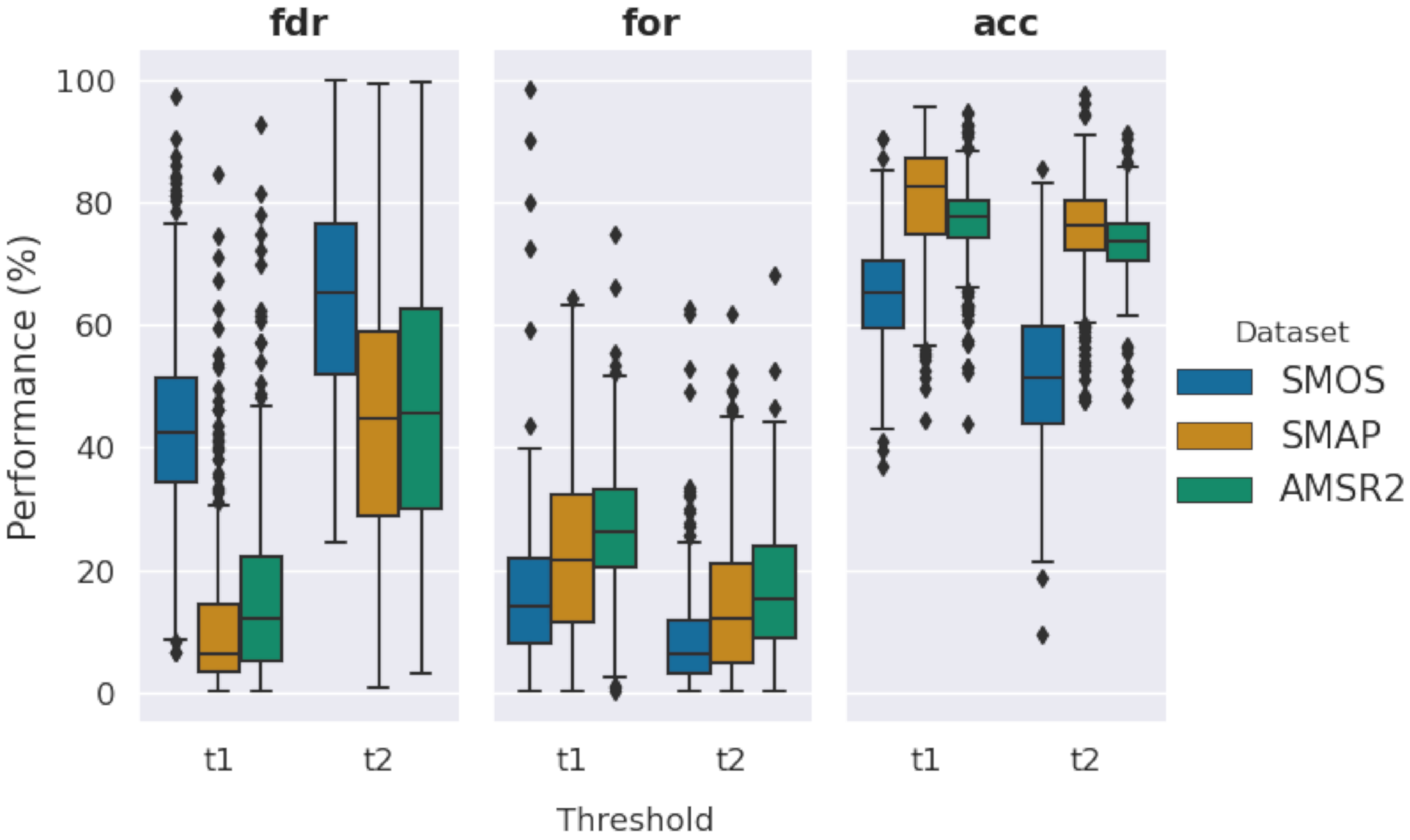
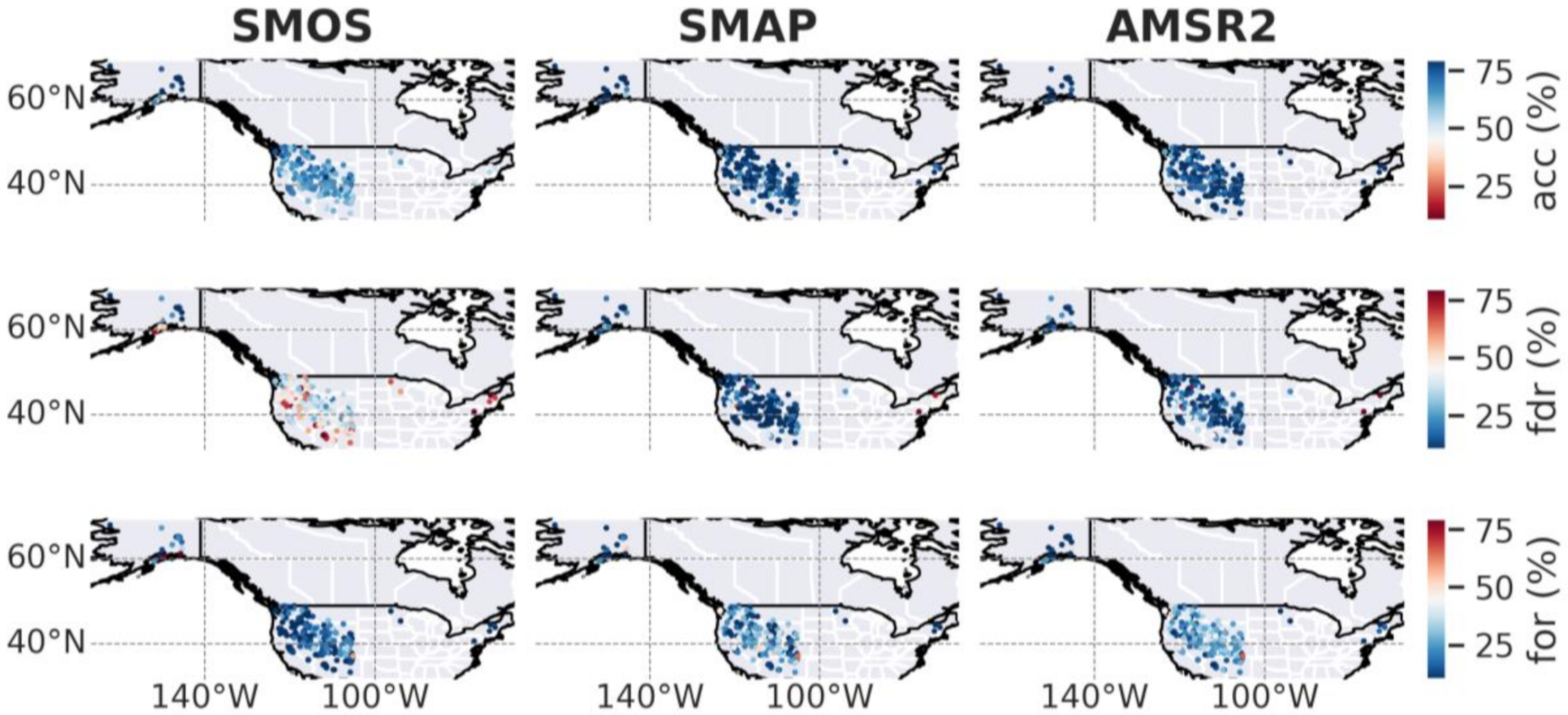
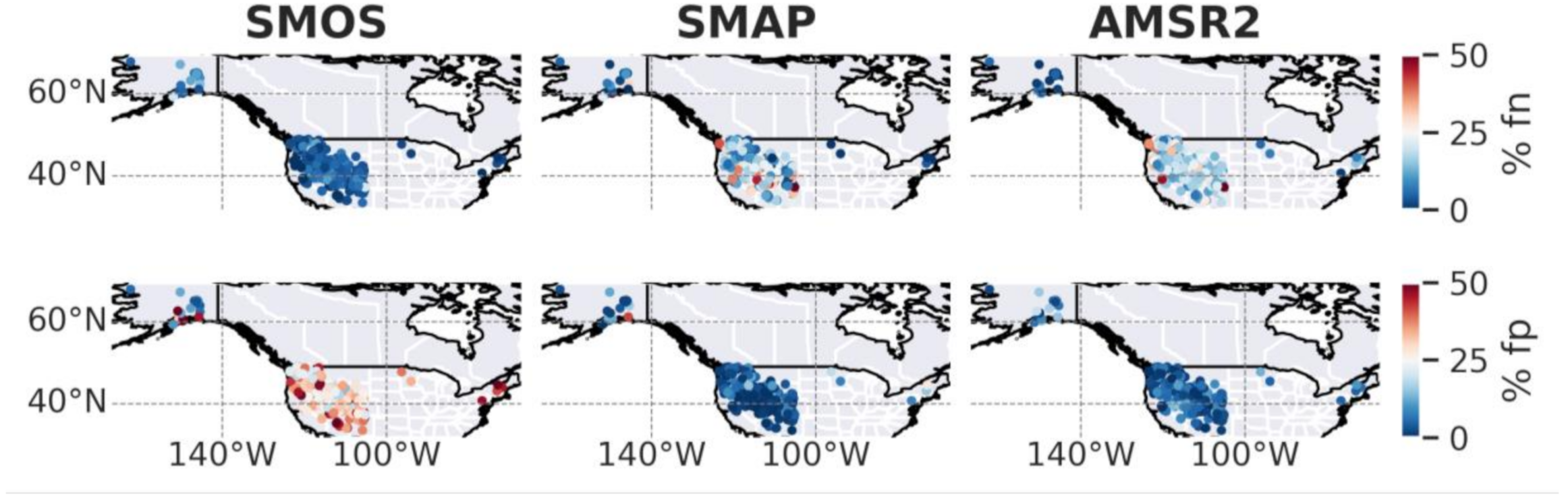
3.2.2. Performance Analysis of the Snow and Ice Flags
4. Results and Discussions
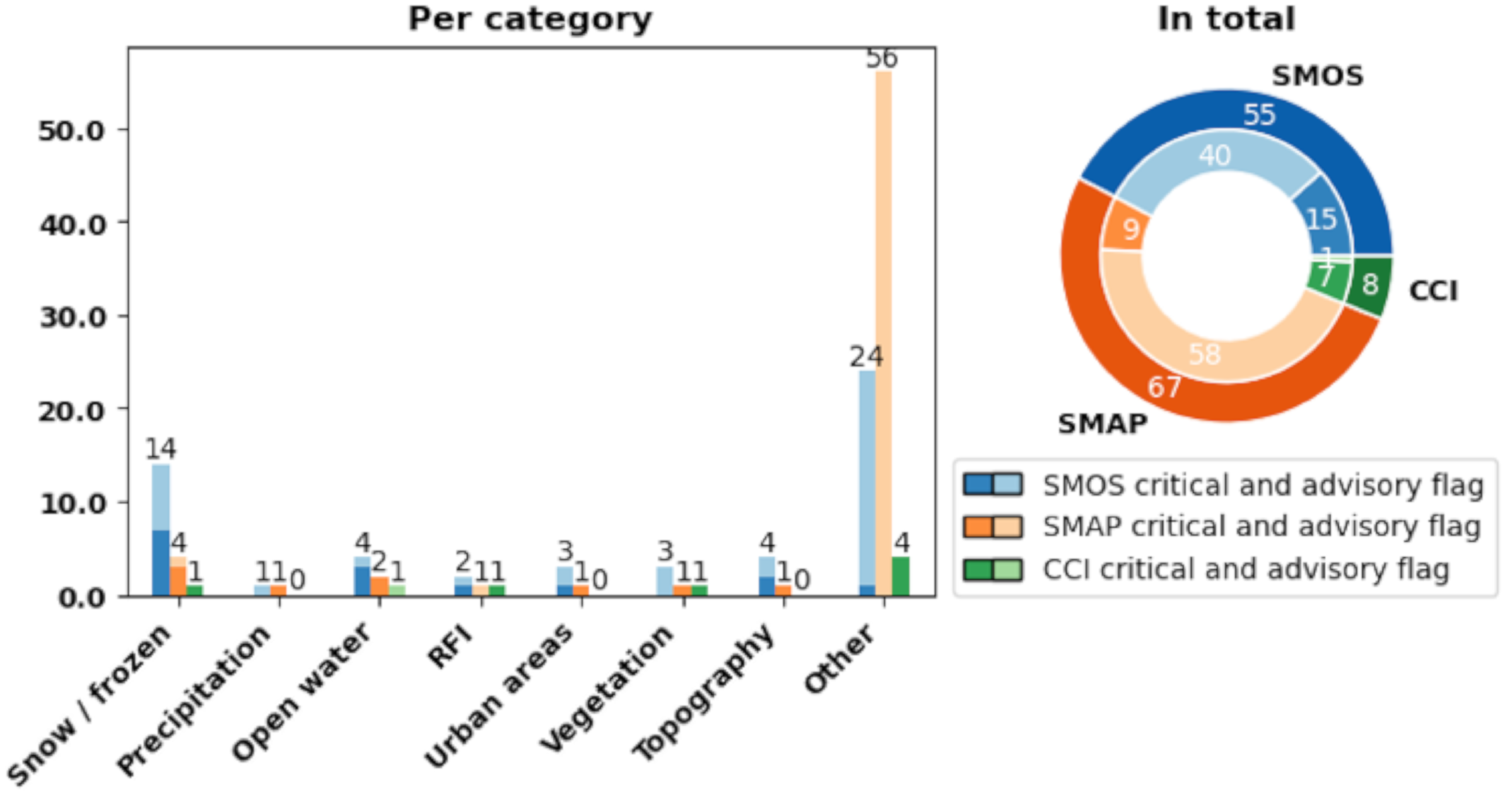
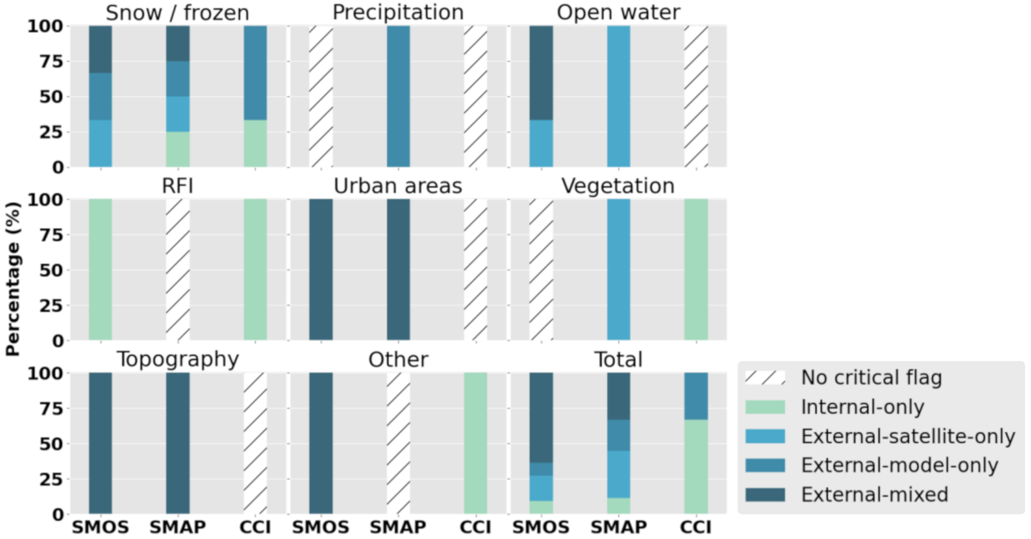
4.1. Differences in Flagging Systems
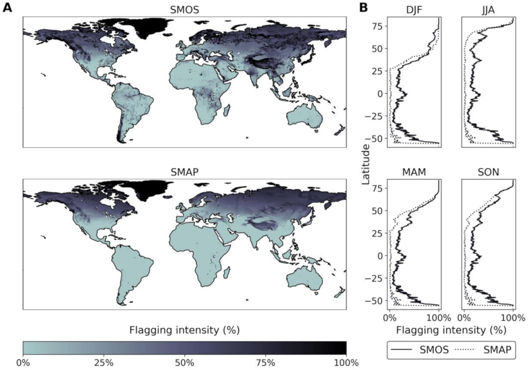
4.2. The Total Flagging Impact on Data Availability
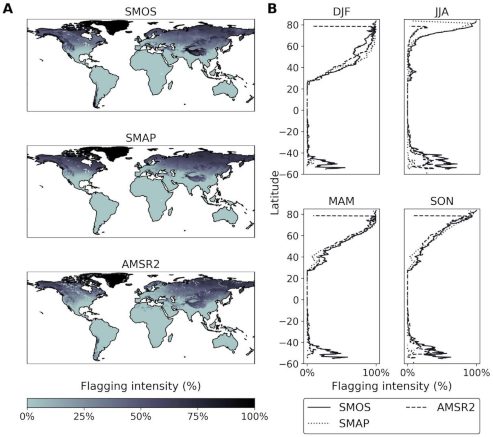
4.3. The New AMSR2-Based Flagging Method in Analyzing the Flagging Intensity
4.4. Performance Evaluation with Ground Observations
5. Conclusions
Author Contributions
Funding
Acknowledgments
Conflicts of Interest
Appendix A

| Flag Category | Total Number of Flags | Number of Critical Flags | Names of Critical Flags | Number of Data Sources of Critical Flags per Category | Names of External Datasets | |||
|---|---|---|---|---|---|---|---|---|
| External- Model-only Datasets | External- Satellite- only Datasets | Eternal- Mixed Datasets | Internal- only Datasets | |||||
| Snow/frozen | 14 | 7 | All wet snow, All mixed snow, Wet snow pollution, Mixed snow pollution, All frost, Frost pollution, All ice | 1 | 1 | 1 | 0 | IFS HRES ECMWF, ESA Ecoclimap 2004, ESA GlobCover V2.3 |
| Precipitation | 1 | 0 | na | na | na | na | na | IFS HRES ECMWF |
| Open water | 4 | 3 | All open water, Heterogeneous OW, All wetlands | 0 | 1 | 2 | 0 | ESA GlobCover V2.3, ESA Ecoclimap 2004, ESRI’s ‘Digital Chart of the World’ dataset |
| RFI | 2 * | 1 | RFI | 0 | 0 | 0 | 1 | na |
| Urban areas | 3 | 1 | All urban | 0 | 0 | 1 | 0 | ESA Ecoclimap 2004 |
| Vegetation | 3 * | 0 | na | na | na | na | na | na |
| Topography | 4 | 2 | Strong topo pollution, Soft topo pollution | 0 | 0 | 2 | 0 | NASA’ s SRTM V2 and USGS GTOPO030 |
| Other | 24 * | 1 | All barren | 0 | 0 | 1 | 0 | ESA Ecoclimap 2004 |
| Total | 55 * | 15 | 1 | 2 | 7 | 1 | ||
| Flag Category | Total Number of Flags | Number of Critical Flags | Names of Critical Flags | Number of Data Sources of Critical Flags per Category | Names of External Datasets | |||
|---|---|---|---|---|---|---|---|---|
| External- Model- only Datasets | External- Satellite- only Datasets | Eternal- Mixed Datasets | Internal- only Datasets | |||||
| Snow/frozen | 4 | 3 | Snow, Permanent Ice, Frozen Ground (from modeled effective soil temperature) | 1 | 1 | 1 | 1 | NOAA IMS database, GMAO GEOS-5, MODIS IGBP |
| Precipitation | 1 | 1 | Precipitation | 1 | 0 | 0 | 0 | GMAO GEOS-5 |
| Open water | 2 | 2 | Static Water, Radar-derived Water Fraction | 0 | 1 | 0 | 0 | MODIS MOD44W database |
| RFI | 1 | 0 | na | 0 | 0 | 0 | 0 | na |
| Urban areas | 1 | 1 | Urban area | 0 | 0 | 1 | 0 | CU GRUMP |
| Vegetation | 1 | 1 | Dense Vegetation | 0 | 1 | 0 | 0 | MODIS NDVI (climatology) and IGBP |
| Topography | 1 | 1 | Mountainous Terrain | 0 | 0 | 1 | 0 | GMTED-2010 |
| Other | 56 | 0 | na | 0 | 0 | 0 | 0 | na |
| Total | 67 | 9 | 2 | 3 | 3 | 1 | ||
| Flag Category | Total Number of Flags | Number of Critical Flags | Names of Critical Flags | Number of Data Sources of Critical Flags per Category | Names of External Datasets | |||
|---|---|---|---|---|---|---|---|---|
| External- Model- only Datasets | External- Satellite- only Datasets | Eternal- Mixed Datasets | Internal- only Datasets * | |||||
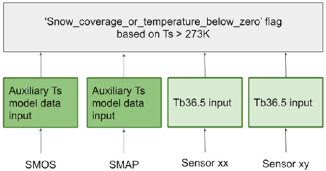
| Snow/frozen | 1 | 1 | Snow Coverage or Temperature Below Zero | 2 | 0 | 0 | 1 | na |
| Precipitation | 0 | 0 | na | 0 | 0 | 0 | 0 | na |
| Open water | 1 | 0 | na | 0 | 0 | 0 | 0 | na |
| RFI | 1 | 1 | na | 0 | 0 | 0 | 1 | na |
| Urban areas | 0 | 0 | na | 0 | 0 | 0 | 0 | na |
| Vegetation | 1 | 1 | Dense vegetation | 0 | 0 | 0 | 1 | na |
| Topography | 0 | 0 | na | 0 | 0 | 0 | 0 | na |
| Other | 4 | 4 | others_no_convergence_in_the_model_thus_no_valid_sm_estimates, soil moisture value exceeds physical boundary, weight of measurement below threshold/data set deemed unreliable, all datasets deemed unreliable | 0 | 0 | 0 | 1 | na |
| Total | 8 | 7 | 2 | 0 | 0 | 4 | ||
References
- Mason, P.J.; Zillman, J.W.; Simmons, A.; Lindstrom, E.J.; Harrison, D.E.; Dolman, H.; Bojinski, S.; Fischer, A.; Latham, J.; Rasmussen, J.; et al. Implementation Plan for the Global Observing System for Climate in Support of the UNFCCC (2010 Update); Word Meteorological Organization (WMO): Geneva, Switzerland, 2010. [Google Scholar]
- LeGates, D.R.; Mahmood, R.; Levia, D.F.; DeLiberty, T.L.; Quiring, S.M.; Houser, C.; Nelson, F.E. Soil moisture: A central and unifying theme in physical geography. Prog. Phys. Geogr. Earth Environ. 2011, 35, 65–86. [Google Scholar] [CrossRef]
- Wagner, W.; Dorigo, W.; De Jeu, R.; Fernandez, D.; Benveniste, J.; Haas, E.; Ertl, M. Fusion of Active and Passive Microwave Observations to Create an Essential Climate Variable Data Record on Soil Moisture. ISPRS Ann. Photogramm. Remote Sens. Spat. Inf. Sci. 2012, 1–7, 315–321. [Google Scholar] [CrossRef]
- Al-Yaari, A.; Wigneron, J.P.; Ducharne, A.; Kerr, Y.; De Rosnay, P.; De Jeu, R.; Govind, A.; Al Bitar, A.; Albergel, C.; Munoz-Sabater, J.; et al. Global-scale evaluation of two satellite-based passive microwave soil moisture datasets (SMOS and AMSR-E) with respect to Land Data Assimilation System estimates. Remote Sens. Environ. 2014, 149, 181–195. [Google Scholar] [CrossRef] [Green Version]
- Dorigo, W.; Wagner, W.; Albergel, C.; Albrecht, F.; Balsamo, G.; Brocca, L.; Chung, D.; Ertl, M.; Forkel, M.; Gruber, A.; et al. ESA CCI Soil Moisture for improved Earth system understanding: State-of-the art and future directions. Remote Sens. Environ. 2017, 203, 185–215. [Google Scholar] [CrossRef]
- Gruber, A.; Dorigo, W.; Crow, W.; Wagner, W. Triple Collocation-Based Merging of Satellite Soil Moisture Retrievals. IEEE Trans. Geosci. Remote Sens. 2017, 55, 6780–6792. [Google Scholar] [CrossRef]
- Liu, Y.Y.; Dorigo, W.; Parinussa, R.; De Jeu, R.; Wagner, W.; McCable, M.; Evans, J.; Van Dijk, A. Trend-preserving blending of passive and active microwave soil moisture retrievals. Remote Sens. Environ. 2012, 123, 280–297. [Google Scholar] [CrossRef]
- Dorigo, W.A.; Chung, D.; Gruber, A.; Hahn, S.; Mistelbauer, T.; Parinussa, R.M.; Paulik, C.; Reimer, C.; der Schalie, R.; de Jeu, R.A.M.; et al. Soil Moisture in “State of the Climate in 2015”. Bull. Am. Meteorol. Soc. 2016, 97, S31–S32. [Google Scholar] [CrossRef] [Green Version]
- Dorigo, W.A.; Scipal, K.; Parinussa, R.M.; Liu, Y.Y.; Wagner, W.; De Jeu, R.A.M.; Naeimi, V. Error characterisation of global active and passive microwave soil moisture datasets. Hydrol. Earth Syst. Sci. 2010, 14, 2605–2616. [Google Scholar] [CrossRef] [Green Version]
- Parinussa, R.; Meesters, A.; Liu, Y.Y.; Dorigo, W.A.; Wagner, W.; De Jeu, R. Error Estimates for Near-Real-Time Satellite Soil Moisture as Derived From the Land Parameter Retrieval Model. IEEE Geosci. Remote Sens. Lett. 2011, 8, 779–783. [Google Scholar] [CrossRef]
- Dorigo, W.; De Jeu, R.; Chung, D.; Parinussa, R.; Liu, Y.; Wagner, W.; Fernández-Prieto, D. Evaluating global trends (1988–2010) in harmonized multi-satellite surface soil moisture. Geophys. Res. Lett. 2012, 39. [Google Scholar] [CrossRef] [Green Version]
- Popp, T.; Hegglin, M.I.; Hollmann, R.; Ardhuin, F.; Bartsch, A.; Bastos, A.; Bennett, V.; Boutin, J.; Brockmann, C.; Buchwitz, M.; et al. Consistency of satellite climate data records for Earth system monitoring. BAMS 2020, D19, 1–68. [Google Scholar] [CrossRef]
- Reichle, R.H.; Koster, R.D.; Dong, J.; Berg, A.A. Global Soil Moisture from Satellite Observations, Land Surface Models, and Ground Data: Implications for Data Assimilation. J. Hydrometeorol. 2004, 5, 430–442. [Google Scholar] [CrossRef]
- Gruhier, C.; De Rosnay, P.; Hasenauer, S.; Holmes, T.R.H.; De Jeu, R.; Kerr, Y.; Mougin, E.; Njoku, E.; Timouk, F.; Wagner, W.; et al. Soil moisture active and passive microwave products: Intercomparison and evaluation over a Sahelian site. Hydrol. Earth Syst. Sci. 2010, 14, 141–156. [Google Scholar] [CrossRef] [Green Version]
- Reichle, R.H.; Koster, R.D.; Liu, P.; Mahanama, S.P.P.; Njoku, E.G.; Owe, M. Comparison and assimilation of global soil moisture retrievals from the Advanced Microwave Scanning Radiometer for the Earth Observing System (AMSR-E) and the Scanning Multichannel Microwave Radiometer (SMMR). J. Geophys. Res. Space Phys. 2007, 112, 1–14. [Google Scholar] [CrossRef]
- Owe, M.; De Jeu, R.; Holmes, T. Multisensor historical climatology of satellite-derived global land surface moisture. J. Geophys. Res. Space Phys. 2008, 113, 1–17. [Google Scholar] [CrossRef]
- Yang, K.; Watanabe, T.; Koike, T.; Li, X.; Fujii, H.; Tamagawa, K.; Ma, Y.; Ishikawa, H. Auto-calibration System Developed to Assimilate AMSR-E Data into a Land Surface Model for Estimating Soil Moisture and the Surface Energy Budget. J. Meteorol. Soc. Jpn. 2007, 85A, 229–242. [Google Scholar] [CrossRef] [Green Version]
- Liu, Y.Y.; Parinussa, R.M.; Dorigo, W.A.; De Jeu, R.A.M.; Wagner, W.; Van Dijk, A.I.J.M.; McCabe, M.; Evans, J.P. Developing an improved soil moisture dataset by blending passive and active microwave satellite-based retrievals. Hydrol. Earth Syst. Sci. 2011, 15, 425–436. [Google Scholar] [CrossRef] [Green Version]
- Dinnat, E.P.; Burgin, M.S.; Colliander, A.; Chae, C.; Cosh, M.; Gao, Y. Intercalibration of Low Frequency Brightness Temperature Measurements for Long-Term Soil Moisture Record. In Proceedings of the IGARSS 2018—2018 IEEE International Geoscience and Remote Sensing Symposium, Valencia, Spain, 22–27 July 2018; pp. 88–91. [Google Scholar] [CrossRef]
- Bindlish, R.; Jackson, T.J.; Chan, S.; Colliander, A.; Kerr, Y. Integration of SMAP and SMOS L-band observations. In Proceedings of the 2017 IEEE International Geoscience and Remote Sensing Symposium (IGARSS), Fort Worth, TX, USA, 23–28 July 2017; pp. 2546–2549. [Google Scholar] [CrossRef] [Green Version]
- Sadri, S.; Pan, M.; Wada, Y.; Vergopolan, N.; Sheffield, J.; Famiglietti, J.S.; Kerr, Y.H.; Wood, E.F. A global near-real-time soil moisture index monitor for food security using integrated SMOS and SMAP. Remote Sens. Environ. 2020, 246, 111864. [Google Scholar] [CrossRef]
- Loew, A.; Stacke, T.; Dorigo, W.A.; De Jeu, R.; Hagemann, S. Potential and limitations of multidecadal satellite soil moisture observations for selected climate model evaluation studies. Hydrol. Earth Syst. Sci. 2013, 17, 3523–3542. [Google Scholar] [CrossRef] [Green Version]
- Grody, N.C. Classification of snow cover and precipitation using the special sensor microwave imager. J. Geophys. Res. Space Phys. 1991, 96, 7423–7435. [Google Scholar] [CrossRef]
- Zhao, T.; Zhang, L.; Jiang, L.; Zhao, S.; Chai, L.; Jin, R. A new soil freeze/thaw discriminant algorithm using AMSR-E passive microwave imagery. Hydrol. Process. 2011, 25, 1704–1716. [Google Scholar] [CrossRef]
- Jin, R.; Zhang, T.; Li, X.; Yang, X.; Ran, Y. Mapping Surface Soil Freeze-Thaw Cycles in China Based on SMMR and SSM/I Brightness Temperatures from 1978 to 2008. Arctic Antarct. Alp. Res. 2015, 47, 213–229. [Google Scholar] [CrossRef] [Green Version]
- Okuyama, A.; Imaoka, K. Intercalibration of Advanced Microwave Scanning Radiometer-2 (AMSR2) Brightness Temperature. IEEE Trans. Geosci. Remote Sens. 2015, 53, 4568–4577. [Google Scholar] [CrossRef]
- Kerr, Y.H.; Waldteufel, P.; Wigneron, J.P.; Delwart, S.; Cabot, F.; Boutin, J.; Escorihuela, M.J.; Font, J.; Reul, N.; Gruhier, C.; et al. The SMOS Mission: New Tool for Monitoring Key Elements ofthe Global Water Cycle. Proc. IEEE 2010, 98, 666–687. [Google Scholar] [CrossRef] [Green Version]
- Entekhabi, D.; Njoku, E.G.; O’Neill, P.E.; Kellogg, K.H.; Crow, W.T.; Edelstein, W.N.; Entin, J.K.; Goodman, S.D.; Jackson, T.J.; Johnson, J.; et al. The Soil Moisture Active Passive (SMAP) Mission. Proc. IEEE 2010, 98, 704–716. [Google Scholar] [CrossRef]
- Imaoka, K.; Kachi, M.; Fujii, H.; Murakami, H.; Hori, M.; Ono, A.; Igarashi, T.; Nakagawa, K.; Oki, T.; Honda, Y.; et al. Global Change Observation Mission (GCOM) for Monitoring Carbon, Water Cycles, and Climate Change. Proc. IEEE 2010, 98, 717–734. [Google Scholar] [CrossRef]
- Kachi, M.; Hori, M.; Maeda, T.; Imaoka, K. Status of validation of AMSR2 on board the GCOM-W1 satellite. In Proceedings of the 2014 IEEE Geoscience and Remote Sensing Symposium, Quebec City, QC, Canada, 13–18 July 2014; pp. 110–113. [Google Scholar]
- Kim, S.; Liu, Y.Y.; Johnson, F.M.; Parinussa, R.M.; Sharma, A. A global comparison of alternate AMSR2 soil moisture products: Why do they differ? Remote Sens. Environ. 2015, 161, 43–62. [Google Scholar] [CrossRef]
- Njoku, E.; Jackson, T.J.; Lakshmi, V.; Chan, T.; Nghiem, S. Soil moisture retrieval from AMSR-E. IEEE Trans. Geosci. Remote Sens. 2003, 41, 215–228. [Google Scholar] [CrossRef]
- Koike, T.; Nakamura, Y.; Kaihotsu, I.; Davaa, G.; Matsuura, N.; Tamagawa, K.; Fujii, H. Development of an advanced microwave scanning radiometer (amsr-e) algorithm for soil moisture and vegetation water content. Proc. Hydraul. Eng. 2004, 48, 217–222. [Google Scholar] [CrossRef] [Green Version]
- Paloscia, S.; Macelloni, G.; Santi, E. Soil Moisture Estimates from AMSR-E Brightness Temperatures by Using a Dual-Frequency Algorithm. IEEE Trans. Geosci. Remote Sens. 2006, 44, 3135–3144. [Google Scholar] [CrossRef]
- Du, J.; Kimball, J.S.; Jones, L.A. Satellite Microwave Retrieval of Total Precipitable Water Vapor and Surface Air Temperature Over Land from AMSR2. IEEE Trans. Geosci. Remote Sens. 2015, 53, 2520–2531. [Google Scholar] [CrossRef]
- Ashcroft, P.; Wentz, F. Algorithm Theoretical Basis Document, AMSR Level 2A Algorithm. RSS Tech. Report 2000, 121, 599B-1; Remote Sensing Systems: Santa Rosa, CA, USA, 2000. [Google Scholar]
- Kerr, Y.H.; Waldteufel, P.; Richaume, P.; Wigneron, J.P.; Ferrazzoli, P.; Mahmoodi, A.; Al Bitar, A.; Cabot, F.; Gruhier, C.; Juglea, S.E.; et al. The SMOS Soil Moisture Retrieval Algorithm. IEEE Trans. Geosci. Remote Sens. 2012, 50, 1384–1403. [Google Scholar] [CrossRef]
- Schmugge, T.; O’Neill, P.E.; Wang, J.R. Passive Microwave Soil Moisture Research. IEEE Trans. Geosci. Remote Sens. 1986, GE-24, 12–22. [Google Scholar] [CrossRef]
- Schmugge, T.J. Remote Sensing of Soil Moisture: Recent Advances. IEEE Trans. Geosci. Remote Sens. 1983, 336–344. [Google Scholar] [CrossRef]
- Van Der Schalie, R.; De Jeu, R.; Parinussa, R.; Rodríguez-Fernández, N.; Kerr, Y.; Al-Yaari, A.; Wigneron, J.P.; Drusch, M. The Effect of Three Different Data Fusion Approaches on the Quality of Soil Moisture Retrievals from Multiple Passive Microwave Sensors. Remote Sens. 2018, 10, 107. [Google Scholar] [CrossRef] [Green Version]
- Jacquette, E.; Al Bitar, A.; Mialon, A.; Kerr, Y.; Quesney, A.; Cabot, F.; Richaume, P. SMOS CATDS level 3 global products over land. In Remote Sensing for Agriculture, Ecosystems, and Hydrology XII, Proceedings of the SPIE Remote Sensing, Toulouse, France, 21–22 September 2010; International Society for Optics and Photonics (SPIE): Bellingham, WA, USA, 2010; Volume 7824, p. 78240K. [Google Scholar] [CrossRef]
- Al Bitar, A.; Leroux, D.J.; Kerr, Y.H.; Merlin, O.; Richaume, P.; Sahoo, A.; Wood, E.F. Evaluation of SMOS Soil Moisture Products Over Continental U.S. Using the SCAN/SNOTEL Network. IEEE Trans. Geosci. Remote Sens. 2012, 50, 1572–1586. [Google Scholar] [CrossRef] [Green Version]
- Al-Bitar, A.; Mialon, A.; Kerr, Y.; Cabot, F.; Richaume, P.; Jacquette, E.; Quesney, A.; Mahmoodi, A.; Tarot, S.; Parrens, M.; et al. The global SMOS Level 3 daily soil moisture and brightness temperature maps. Earth Syst. Sci. Data 2017, 9, 293–315. [Google Scholar] [CrossRef] [Green Version]
- Kerr, Y.; Jacquette, E.; Al Bitar, A.; Cabot, F.; Mialon, A.; Richaume, P.; Quesney, A.; Berthon, L. CATDS SMOS L3 Soil Moisture Retrieval Processor: Algorithm Theoretical Baseline Document (ATBD); CESBIO: Toulouse, France, 2013; Ref.: SO-TN-CBSA-GC-0029. [Google Scholar]
- Kerr, Y.; Richaume, P.; Waldteufel, P.; Wigneron, J.P.; Ferrazzoli, P. SMOS Level 2 Processor for Soil Moisture Algorithm Theoretical Based Document (ATBD); Tech. Report, ESA No.: SO-TN-ARR-L2PP-0037, Issue 3.10; IPSL-Service d’Aéronomie; INRAEPHYSE; Reading University; Tor Vergata University: Toulouse, France, 2017. [Google Scholar]
- Panciera, R.; Walker, J.P.; Jackson, T.J.; Gray, D.A.; Tanase, M.A.; Ryu, D.; Monerris, A.; Yardley, H.; Rudiger, C.; Wu, X.; et al. The Soil Moisture Active Passive Experiments (SMAPEx): Toward Soil Moisture Retrieval from the SMAP Mission. IEEE Trans. Geosci. Remote Sens. 2014, 52, 490–507. [Google Scholar] [CrossRef]
- Chan, S.K.; Bindlish, R.; O’Neill, P.E.; Njoku, E.; Jackson, T.; Colliander, A.; Chen, F.; Burgin, M.; Dunbar, S.; Piepmeier, J.; et al. Assessment of the SMAP Passive Soil Moisture Product. IEEE Trans. Geosci. Remote Sens. 2016, 54, 4994–5007. [Google Scholar] [CrossRef]
- Gruber, A.; Scanlon, T.; Van Der Schalie, R.; Wagner, W.; Dorigo, W. Evolution of the ESA CCI Soil Moisture climate data records and their underlying merging methodology. Earth Syst. Sci. Data 2019, 11, 717–739. [Google Scholar] [CrossRef] [Green Version]
- Wagner, W.; Lemoine, G.; Rott, H. A Method for Estimating Soil Moisture from ERS Scatterometer and Soil Data. Remote Sens. Environ. 1999, 70, 191–207. [Google Scholar] [CrossRef]
- Dorigo, W.A.; Wagner, W.; Hohensinn, R.; Hahn, S.; Paulik, C.; Xaver, A.; Gruber, A.; Drusch, M.; Mecklenburg, S.; Van Oevelen, P.; et al. The International Soil Moisture Network: A data hosting facility for global in situ soil moisture measurements. Hydrol. Earth Syst. Sci. 2011, 15, 1675–1698. [Google Scholar] [CrossRef] [Green Version]
- Dorigo, W.A.; Xaver, A.; Vreugdenhil, M.; Gruber, A.; Hegyiová, A.; Sanchis-Dufau, A.; Zamojski, D.; Cordes, C.; Wagner, W.; Drusch, M. Global Automated Quality Control of In Situ Soil Moisture Data from the International Soil Moisture Network. Vadose Zone J. 2013, 12, 3. [Google Scholar] [CrossRef]
- Schaefer, G.L.; Paetzold, R.F. SNOTEL (SNOwpack TELemetry) and SCAN (soil climate analysis network). In Automated Weather Stations for Applications in Agriculture and Water Resources Management: Current Use and Future Perspectives; University of Nebraska: Lincoln, NE, USA, 2001; Volume 1074, pp. 187–194. [Google Scholar]
- Chung, D.; Dorigo, W.; De Jeu, R.A.M.; Kidd, R.; Wagner, W. ESA Climate Change Initiative Plus—Soil Moisture Product Specification Document (PSD); Earth Observation Data Centre for Water Resources Monitoring (EODC) GmbH: Vienna, Austria; VanderSat: Haarlem, The Netherlands; CESBIO: Toulouse, France, 2019; D1.2.1 Version 4.5. [Google Scholar]
- Holmes, T.R.H.; De Jeu, R.A.M.; Owe, M.; Dolman, A.J. Land surface temperature from Ka band (37 GHz) passive microwave observations. J. Geophys. Res. Space Phys. 2009, 114, D4. [Google Scholar] [CrossRef] [Green Version]
- O’Neill, P.E.; Njoku, E.G.; Jackson, T.J.; Chan, S.; Bindlish, R. SMAP Algorithm Theoretical Basis Document: Level 2 & 3 Soil Moisture (Passive) Data Products; NASA Jet Propulsion Laboratory, California Institute of Technology: Pasadena, CA, USA, 2018; JPL D-66480, Revision D. [Google Scholar]
- De Jeu, R.A.M. Retrieval of Land Surface Parameters Using Passive Microwave Remote Sensing. Ph.D. Thesis, Vrije Universiteit Amsterdam, Amsterdam, The Netherlands, February 2003. [Google Scholar]
- Rautiainen, K.; Lemmetyinen, J.; Schwank, M.; Kontu, A.; Ménard, C.B.; Mätzler, C.; Drusch, M.; Wiesmann, A.; Ikonen, J.; Pulliainen, J. Detection of soil freezing from L-band passive microwave observations. Remote Sens. Environ. 2014, 147, 206–218. [Google Scholar] [CrossRef]
- England, A.; Galantowicz, J.; Zuerndorfer, B.W. A volume scattering explanation for the negative spectral gradient of frozen soil. In Proceedings of the IGARSS’91 Remote Sensing: Global Monitoring for Earth Management, Espoo, Finland, 3–6 June 1991; pp. 1175–1177. [Google Scholar] [CrossRef]
- Zuerndorfer, B.; England, A.; Dobson, M.; Ulaby, F. Mapping freeze/thaw boundaries with SMMR data. J. Agric. For. Meteorol. 1990, 52, 199–225. [Google Scholar] [CrossRef] [Green Version]
- Zuerndorfer, B.; England, A.; Ulaby, F. An Optimized Approach to Mapping Freezing Terrain with SMMR Data. In Proceedings of the 10th Annual International Symposium on Geoscience and Remote Sensing, College Park, MD, USA, 20–24 May 1990; pp. 1153–1156. [Google Scholar] [CrossRef]
- Jin, Y.Q. Simulation of a multi-layer model of dense scatterers for anomalous scattering signatures from SSM/I snow data. Int. J. Remote Sens. 1997, 18, 2531–2538. [Google Scholar] [CrossRef]
- Grody, N.C.; Basist, A.N. Interpretation of SSM/I measurements over Greenland. IEEE Trans. Geosci. Remote Sens. 1997, 35, 360–366. [Google Scholar] [CrossRef]
- Foster, J.L.; Chang, A.T.C.; Hall, D.K.; Kelly, R. Seasonal snow extent and snow mass in South America using SSMI passive microwave data (1979–2006). Remote Sens. Environ. 2009, 113, 291–305. [Google Scholar] [CrossRef] [Green Version]
- Durand, M.; Kim, E.J.; Margulis, S.A. Quantifying Uncertainty in Modeling Snow Microwave Radiance for a Mountain Snowpack at the Point-Scale, Including Stratigraphic Effects. IEEE Trans. Geosci. Remote Sens. 2008, 46, 1753–1767. [Google Scholar] [CrossRef]
- Grody, N. Relationship between snow parameters and microwave satellite measurements: Theory compared with Advanced Microwave Sounding Unit observations from 23 to 150 GHz. J. Geophys. Res. Space Phys. 2008, 113. [Google Scholar] [CrossRef]
- Granger, S.; Kraif, O.; Ponton, C.; Antoniadis, G.; Zampa, V. Integrating learner corpora and natural language processing: A crucial step towards reconciling technological sophistication and pedagogical effectiveness. Recall 2007, 19, 252–268. [Google Scholar] [CrossRef]


| Snow/Frozen Soil Fraction | Action |
|---|---|
| 0.00–0.05 | flag for recommended quality and retrieve soil moisture |
| 0.05–0.50 | flag for uncertain quality and attempt to retrieve soil moisture |
| 0.50–1.00 | flag but do not retrieve soil moisture |
| SMOS | SMAP | CCI | ||
|---|---|---|---|---|
| Total number of flags | 55 * | 67 | 8 | |
| Number of critical flags | 15 | 9 | 7 | |
| Names of critical flags | All wet snow, All mixed snow, Wet snow pollution, Mixed snow pollution, All frost, Frost pollution, All ice, All open water, Heterogeneous OW, All wetlands, RFI, All urban, Strong topo pollution, Soft topo pollution, All barren | Snow, Permanent Ice, Frozen Ground (from modeled effective soil temperature), Precipitation, Static Water, Radar-derived Water Fraction, Urban area, Dense Vegetation, Mountainous Terrain | Snow Coverage or Temperature Below Zero, Dense vegetation, others_no_convergence_in_the_model_thus_no_valid_sm_estimates, soil moisture value exceeds physical boundary, weight of measurement below threshold / data set deemed unreliable, all datasets deemed unreliable, RFI | |
| Number of data sources of critical flags | Internal-only datasets | 1 | 1 | 4 ** |
| External-model-only datasets | 1 | 2 | 2 | |
| External-satellite-only datasets | 2 | 3 | 0 | |
| External-mixed datasets | 7 | 3 | 0 | |
| Names of external datasets | IFS HRES ECMWF, ESA GlobCover V2.3, ESA Ecoclimap 2004, ESRI’s ‘Digital Chart of the World’ dataset, NASA’ s SRTM V2, USGS GTOPO030 | NOAA IMS database, GMAO GEOS-5, MODIS NDVI, IGBP and MOD44W database, GMTED-2010, GSHHG | na | |
| Number and type of advisory flags | S_Tree_1 Components Forest Cover and Soil Cover, All 34 Product Science Flags, All 3 Retrieval flags | Coastal Proximity, All 5 tb_qual_flags | na | |
Publisher’s Note: MDPI stays neutral with regard to jurisdictional claims in published maps and institutional affiliations. |
© 2020 by the authors. Licensee MDPI, Basel, Switzerland. This article is an open access article distributed under the terms and conditions of the Creative Commons Attribution (CC BY) license (http://creativecommons.org/licenses/by/4.0/).
Share and Cite
van der Vliet, M.; van der Schalie, R.; Rodriguez-Fernandez, N.; Colliander, A.; de Jeu, R.; Preimesberger, W.; Scanlon, T.; Dorigo, W. Reconciling Flagging Strategies for Multi-Sensor Satellite Soil Moisture Climate Data Records. Remote Sens. 2020, 12, 3439. https://0-doi-org.brum.beds.ac.uk/10.3390/rs12203439
van der Vliet M, van der Schalie R, Rodriguez-Fernandez N, Colliander A, de Jeu R, Preimesberger W, Scanlon T, Dorigo W. Reconciling Flagging Strategies for Multi-Sensor Satellite Soil Moisture Climate Data Records. Remote Sensing. 2020; 12(20):3439. https://0-doi-org.brum.beds.ac.uk/10.3390/rs12203439
Chicago/Turabian Stylevan der Vliet, Mendy, Robin van der Schalie, Nemesio Rodriguez-Fernandez, Andreas Colliander, Richard de Jeu, Wolfgang Preimesberger, Tracy Scanlon, and Wouter Dorigo. 2020. "Reconciling Flagging Strategies for Multi-Sensor Satellite Soil Moisture Climate Data Records" Remote Sensing 12, no. 20: 3439. https://0-doi-org.brum.beds.ac.uk/10.3390/rs12203439