Thick Cloud Removal of Remote Sensing Images Using Temporal Smoothness and Sparsity Regularized Tensor Optimization

Abstract

In remote sensing images, the presence of thick cloud accompanying shadow can affect the quality of subsequent processing and limit the scenarios of application. Hence, to make good use of such images, it is indispensable to remove the thick cloud and cloud shadow as well as recover the cloud-contaminated pixels. Generally, the thick cloud and cloud shadow element are not only sparse but also smooth along the spatial horizontal and vertical direction, while the clean element is smooth along the temporal direction. Guided by the above insight, a novel thick cloud removal method for remote sensing images based on temporal smoothness and sparsity regularized tensor optimization (TSSTO) is proposed in this paper. Firstly, the sparsity norm is utilized to boost the sparsity of the cloud and cloud shadow element, and unidirectional total variation (UTV) regularizers are applied to ensure the smoothness in different directions. Then, through thresholding, the cloud mask and the cloud shadow mask can be acquired and used to guide the substitution. Finally, the reference image is selected to reconstruct details of the repairing area. A series of experiments are conducted both on simulated and real cloud-contaminated images from different sensors and with different resolutions, and the results demonstrate the potential of the proposed TSSTO method for removing cloud and cloud shadow from both qualitative and quantitative viewpoints.

1. Introduction

Remote sensing images have been widely used in many research and application fields, such as classification [1,2], object detection [3], and urban geographical mapping [4]. However, remote sensing images are often affected by cloud cover. According to the report from the International Satellite Cloud Climatology Project (ISCCP) [5], the annual global average cloud cover is up to 66%. Thick clouds usually cover up the earth’s surface information, so the information on cloud-contaminated pixels are always inaccurate or missing, which notably affects usability and limits further analysis of remote sensing images. Since thick cloud cover is inevitable for optical remote sensing images and influences the subsequent processing, using appropriate methods to remove the cloud and cloud shadow is imperative.

Thick cloud leads to loss of land cover information, so the main task of removing thick cloud is to recover the cloud-contaminated pixels using available information. To this end, many methods for thick cloud removal have been proposed in the last few decades. According to the source of information exploited to reconstruct the cloud-cover area, the existing methods can be classified into spatial information-based methods, spectral information-based methods, and temporal information-based methods.

■

Spatial information-based methods

The spatial information-based methods are dedicated to recovering the cloud-contaminated pixels by making full use of the information from the cloud-free area in the image to be repaired. Missing pixel interpolation is the elementary method of these methods [6,7], which is only suitable for recovering tiny missing areas but cannot deal with the large area absence. To remedy this limitation, many techniques have been introduced [8,9,10]. Criminisi inpainting [8] fulfilled the missing area within the target image and reconstructed pixels in an appropriate order patch by patch. Bandelet-based inpainting exploited the spectro-geometrical information in the cloud-free parts of the cloud-contaminated image [9]. Maximum a posteriori (MAP)-based method got the cloud-free image using apriori knowledge and gradient descent optimization [10]. Recently, Cheng et al. [11] and Zeng et al. [12] proposed methods using similar pixel locations and global optimization to get a seamless repaired image. Additionally, tensor completion-based methods [13] such as FaLRTC and HaLRTC also can be generalized to cloud removal in remotely sensed images. However, spatial information-based methods can only get a visually plausible cloud-free image when the cloud-contaminated area is small. Once the missing area becomes large, these methods’ results are not practicable for subsequent quantitative analysis and applications [14].

■

Spectral information-based methods

For many multispectral and hyperspectral images, some areas can be contaminated in certain bands, while other bands’ information can be intact. The main idea of the spectral information-based methods is to use information from unaffected and unspotted bands to reconstruct the missing bands. For instance, many algorithms modelled the relationship between the Moderate Resolution Imaging Spectrora-diometer (MODIS) band 7 and MODIS band 6 to remove the periodic strips in MODIS band 6 [15,16,17]. These methods can be applied to cloud removal, as the main task of cloud removal is to reconstruct the missing data. Compared to the visible wavelengths, short-wavelength infrared (SWIR) wavelengths can penetrate through cloud, which allows detection of ground surface information under cloud cover. On this premise, Li et al. [18] exploited shortwave infrared information to obtain haze-free imagery. For Landsat images, Zhang et al. [19] represented a haze optimized transformation (HOT) method that corrected the visible bands radiometrically and removed the cloud in images. In recent years, Malek et al. [20] harnessed autoencoder networks to reconstruct the cloud area of the multispectral image. Although spectral information-based methods can make better use of auxiliary information than spatial information-based methods, they are invalid when thick clouds contaminate all the bands.

■

Temporal information-based methods

In temporal information-based methods, there has to be at least one reference image which covers the cloud area in the target image (the image to be repaired). As the auxiliary information contained in the reference image can be utilized to reconstruct the cloud area in the target image, the effectiveness of these methods is ensured. The primary method is managing to build a linear relationship between cloud-contaminated pixels in the target image and corresponding pixels in the reference image [21,22,23]. However, the linear regression model has a finite ability to obtain the seamless reconstructed image. To tackle this issue, many tactics have been figured out to lower the radiometric differences between the original cloud-free area and the area recovered by regression. For example, Zeng et al. [24] and Li et al. [5] proposed different residual correction methods to guarantee seamless reconstruction results. As the land cover change increases the difficulty of cloud removal, Markov random field global function [14] and patch-based information reconstruction [25,26] were proposed to minimize the effect of the land cover changes. Meanwhile, the sparse representation techniques have also been applied to cloud removal. Sparsity assumes that a signal has only few non-zero points, and all other sampling points are zero (or around zero). Regarding when the cloud is sparse and the cloud-free element possesses the characteristic of low-rank, Wen et al. [27] and Zhang et al. [28] introduced the robust principal component analysis (RPCA) into the cloud removal task. By applying discrepant RPCA, they presented two-pass RPCA (TRPCA) and group-sparsity constrained RPCA (GRPCA) to detect and remove the cloud. As a frequently used sparse representation method, dictionary learning was also employed to remove the cloud in remote sensing images [29,30,31,32]. Similar to sparse representation, Li et al. [33] proposed a nonnegative matrix factorization-based method but the coefficients of which were not always sparse. Furthermore, many researchers expanded this series of methods from a two-dimensional matrix to high-dimensional tensor and combined them with total variation (TV). Ng et al. [34] and Cheng et al. [35] designed adaptive weighted tensor completion methods to recover the cloud-contaminated pixels. Ji et al. [36] suggested a nonlocal tensor completion method to restore the missing area. Chen et al. [37] proposed a low-rank sparsity decomposition method regularized by total variation, called TVLRSDC, which could remove the cloud and cloud shadow simultaneously. As deep learning has shown its tremendous potential in image processing, Zhang et al. [38] made use of a deep convolutional neural network to extract multiscale features and recover the absent information. Generally, the temporal information-based methods can obtain satisfactory results, as long as the spectral difference and the land cover change are not too discrepant between the target image and reference image.

Different from the methods as mentioned above, this paper proposes a novel tensor optimization model based on temporal smoothness and sparse representation (TSSTO) for thick cloud and cloud shadow removal in remote sensing images. For the sake of clear illustration, the rest of this paper use shorthand “horizontal” and” vertical” to represent “spatial horizontal” and “spatial vertical”, respectively. Meanwhile, “shadow” signifies “cloud shadow”, and “cloud/shadow” represents the cloud and shadow in images. The proposed TSSTO method is mainly on the basis of the discriminatively intrinsic features that the cloud/shadow is often sparse and smooth along the horizontal and vertical direction in images, while the clean images are smooth along the temporal direction between images.

The main contributions of this paper could be listed as follows:

• This paper ensures temporal smoothness by unidirectional total variation regularizer. Considering the gradient along the temporal direction between images in the clean element is smaller than that in the cloud/shadow element, unidirectional total variation (UTV) regularizer along the temporal direction is exploited to constrain the temporal smoothness of the clean element.
• Group sparsity is used to enhance the sparsity of the cloud/shadow, and two unidirectional total variation regularizers along the horizontal and vertical direction are designed to deal with the large cloud/shadow area. This scheme enables TSSTO better to remove both the large and small cloud-contaminated area.

The rest of this paper is organized as follows. In Section 2, the proposed TSSTO method and implementation details are introduced. In Section 3, a series of experiments are conducted and analyzed. The conclusions of this paper and the direction of future work are reported in Section 4.

2. Methodology

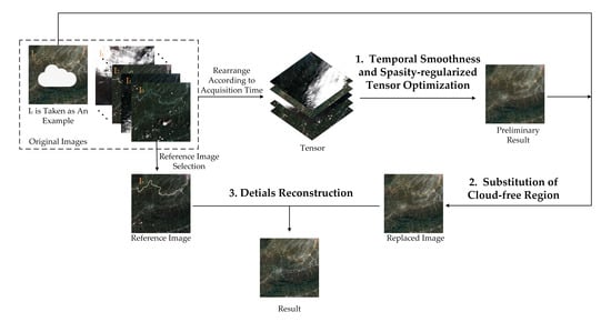
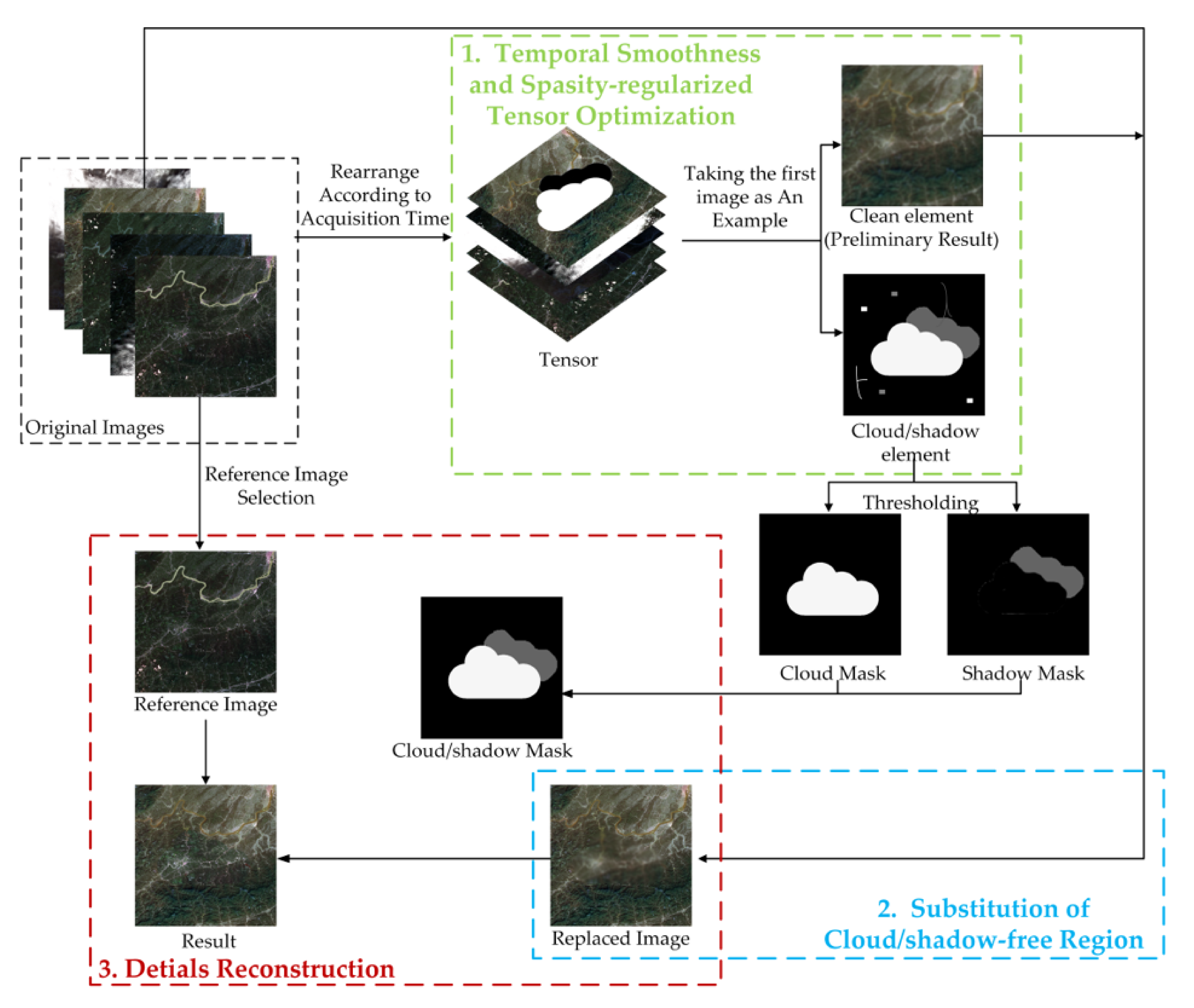
Usually, the cloud/shadow element would be sparse and smooth along the horizontal and vertical direction, while the clean images would be smooth along the temporal direction, except when the majority of images are covered by cloud, or there are sudden significant surface changes between images. Based on this prior knowledge, the cloud/shadow element and the clean element can be obtained by the proposed temporal smoothness and sparsity regularized model. Concretely, the cloud/shadow element is constrained by the group sparsity and two UTV regularizers, and the UTV regularizer guarantees the temporal smoothness of the clean element along the temporal direction. As shown in Figure 1, the proposed TSSTO method contains three steps: firstly, the images are arranged to a tensor according to the acquisition time. By executing the proposed model that is introduced in Section 2.1.1, the cloud/shadow element and the clean element can be acquired, and the clean element can be seen as the preliminary recovery results. Secondly, thresholds are applied to the cloud/shadow element to get the cloud mask and shadow mask. Then, according to the cloud/shadow mask, the clean area in the original images is substituted for the corresponding area in the preliminary recovery result. This step together with the tensor optimization step is called TOS. Thirdly, to recover subtle texture information, the details of the cloud/shadow area are recovered by information cloning. It is worth noting that the cloud/shadow will be removed only when the clean complementary information is available in the multitemporal images. The input of the proposed TSSTO method is a sequence of images that cover the same area, and the cloud/shadow masks could be provided or not.

2.1. Tensor Optimization Based on Temporal Smoothness and Sparsity

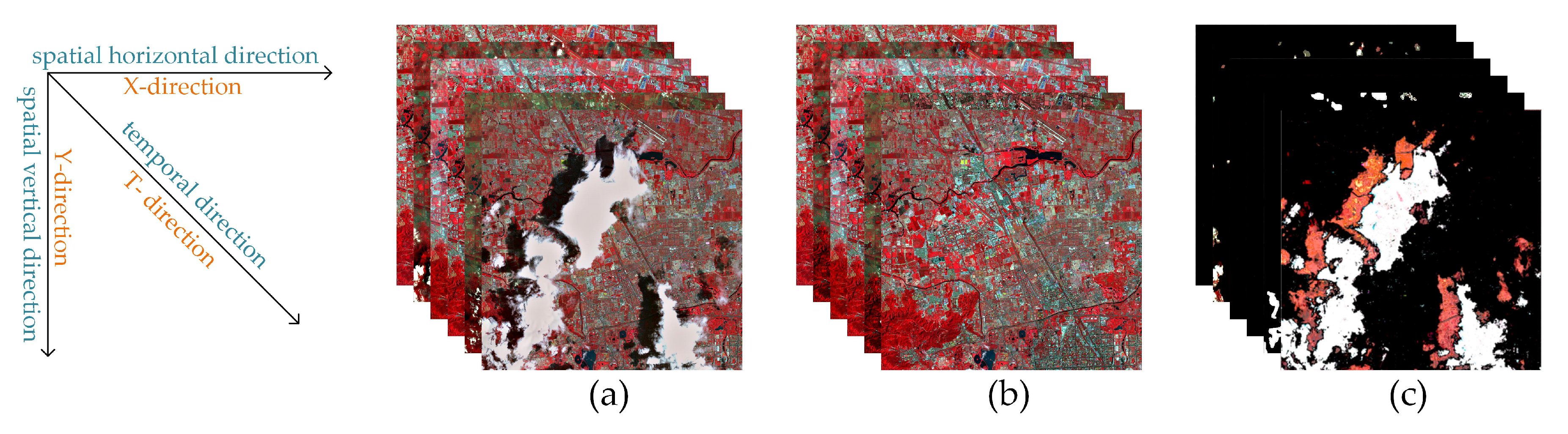
Generally, the cloud/shadow element is supposed to be sparser than the clean element in the cloud-contaminated images, unless the cloud cover obscures the most parts of images. Therefore, group sparsity is used to promote the sparsity of the cloud/shadow element. To better explain the UTV regularizers, Figure 2 shows the original cloud-contaminated images, clean element, and the cloud/shadow element. Figure 3, Figure 4 and Figure 5 show the histogram of the absolute values of the gradients in different directions.

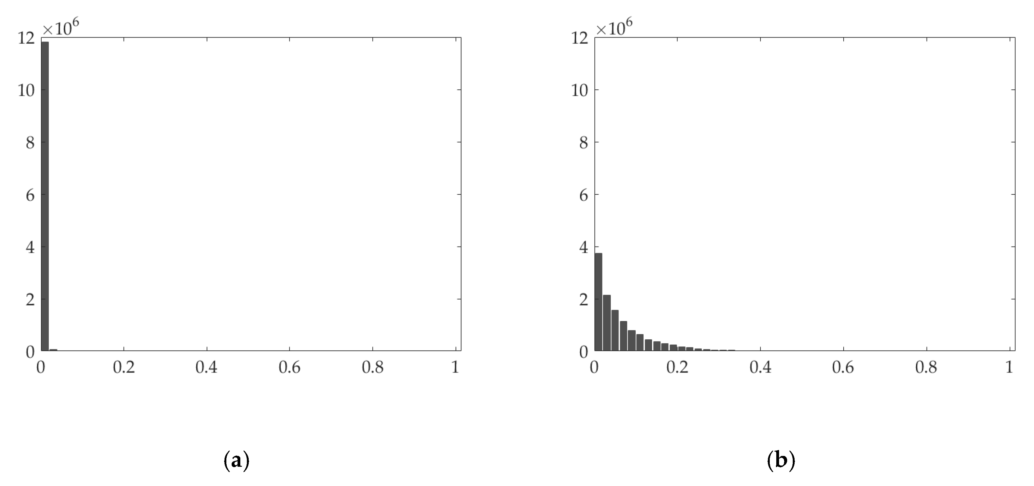
As shown in Figure 3b and Figure 4b, the derivatives of the clean element are not sparse along the horizontal and vertical directions. Conversely, the derivatives of the cloud/shadow element are sparse along the horizontal and vertical direction, which can be seen from Figure 3a and Figure 4a. Hence, we constrain the horizontal and vertical gradient of the cloud/shadow element to be small in horizontal and vertical directions, thereby extracting the cloud/shadow element. In the temporal direction, as shown in Figure 5, the gradient of the clean images is usually small, while the temporal gradient of the cloud/shadow element tends to be extraordinarily finite or extremely large. This graph indicates essential information of the cloud/shadow is in the part of the large gradient. By constraining the temporal gradient of the clean element to be small, the cloud/shadow element can be obtained, and the general spectrum of the cloud/shadow area can be recovered in the clean element.

2.1.1. Temporal Smoothness and Sparsity Regularized Model

Mathematically, a single remote sensing image can be represented as $I\in {\mathbb{R}}^{m\times n\times b}$ where $m$ and $n$ denote the numbers of rows and columns, and $b$ denotes the number of spectral bands, respectively. Given a series of remote sensing images, according to the acquisition time, they can be arranged into a tensor $\in$${\mathbb{R}}^{m\times n\times t}$, where $t$ denotes the numbers of images, thereby processing images band by band.

Supposing that $\mathcal{D},\mathcal{C},$ and $\mathcal{B}\in {\mathbb{R}}^{m\times n\times t},$ respectively, represent the original cloud-contaminated images, the cloud/shadow element, and the clean element, the proposed cloud removal model can be formulated as

$$\begin{gathered} arg \underset{\mathcal{B},\mathcal{C}}{\min } {\lambda }_1\parallel {\nabla }_x{\mathcal{C}\parallel }_1+{\lambda }_2\parallel {\nabla }_y{\mathcal{C}\parallel }_1+{\lambda }_3\parallel {\nabla }_z{\mathcal{B}\parallel }_1+{\lambda }_4\parallel {\mathcal{C}\parallel }_{2,1} \\ \mathrm{s}.\mathrm{t}. \mathcal{D}=\mathcal{B}+\mathcal{C}, \mathcal{B}\ge 0. \end{gathered}$$

(1)

where ${\nabla }_x, {\nabla }_y, \mathrm{and} {\nabla }_z$ denote the derivative operators of horizontal dimension, vertical dimension, and temporal dimension, respectively. ${\lambda }_1, {\lambda }_2, {\lambda }_3$, $\mathrm{and} {\lambda }_4$ are the parameters that adjust the weights of different information sources.

As the derivatives of the cloud/shadow element along the horizontal and vertical direction are sparser than clean element, which can be seen in Figure 3 and Figure 4, the unidirectional total variation (UTV) regularizers $\parallel {\nabla }_x{\mathcal{C}\parallel }_1$ and $\parallel {\nabla }_y{\mathcal{C}\parallel }_1$ are utilized to enhance the smoothness of the cloud/shadow element.

Generally, the cloud/shadow elements usually have large gradients in the temporal domain between images as a result of the randomness of the thick cloud. Conversely, the clean element owns small temporal gradients because the features of land cover just change slightly according to a particular trend over time. Therefore, the term $\parallel {\nabla }_z{\mathcal{B}\parallel }_1$ to constrain the temporal smoothness is applied in Equation (1).

The term $\parallel {\mathcal{C}\parallel }_{2,1}$ represents the group sparsity of the cloud/shadow. When the cloud is not massive, the cloud/shadow can be seen as a sparse term approximately. Commonly, the cloud/shadow element is sparser than the clean element for a useful image. Hence, $\parallel {\mathcal{C}\parallel }_{2,1}$, a ${\ell }_{2,1}$ norm, is used to promote the group sparsity of the cloud/shadow element. Concretely, for a matrix $X$, $X_{2,1}$ is defined as

$$\parallel {X\parallel }_{2,1}={\displaystyle \sum }_{i=1}^s\parallel x_{g_i}{\parallel }_2$$

(2)

where $g_i$ denotes the ith group of the variable $X$ and $s$ is the number of groups. For a tensor $\mathcal{C}$, $\parallel {\mathcal{C}\parallel }_{2,1}$ is defined as

$$\parallel {\mathcal{C}\parallel }_{2,1}=\parallel {\mathrm{unfold}}_1{\left(\mathcal{C}\right)\parallel }_{2,1}$$

(3)

2.1.2. Optimization of the Proposed Model

The proposed model formulated by Equation (1) is a convex optimization problem. This paper utilizes the alternating direction method of multipliers (ADMM) framework [39] to solve the proposed model. ADMM framework can convert the complex multivariable optimization task to a few simple subtasks. In the ADMM framework, the variables are updated iteratively, and the optimization problem is solved by alternately optimizing one variable with other variables fixed. To fit the ADMM framework, the auxiliary variables, $\mathcal{A}, \mathcal{H}, \mathcal{V}, \mathrm{and} \mathcal{T}$ are introduced and the constrained Equation (1) is rewritten to

$$\begin{gathered} arg \underset{\mathcal{A},\mathcal{C},\mathcal{H},\mathcal{V},\mathcal{T}}{\min } {\lambda }_1\parallel {\mathcal{H}\parallel }_1+{\lambda }_2\parallel {\mathcal{V}\parallel }_1+{\lambda }_3\parallel {\mathcal{T}\parallel }_1+{\lambda }_4\parallel {\mathcal{A}\parallel }_{2,1} \\ \mathrm{s}.\mathrm{t}. \mathcal{A}=\mathcal{C} \\ \hspace{1em}\hspace{1em} \mathcal{H}={\nabla }_x\mathcal{C} \\ \hspace{1em}\hspace{1em} \mathcal{V}={\nabla }_y\mathcal{C} \\ \hspace{1em}\hspace{1em} \mathcal{T}={\nabla }_z \left(\mathcal{D}-\mathcal{C}\right) \\ \hspace{1em}\hspace{1em} \mathcal{D}\ge \mathcal{C} , \end{gathered}$$

(4)

Then the Augmented Lagrange Multipliers (ALM) method [40] is employed to optimize the Equation (4). ALM replaces constrained optimization problem by an unconstrained problem using Lagrange multiplier and adds a penalty term to the objective. Let $\mathcal{Y}=\left[{\mathcal{Y}}_1,{\mathcal{Y}}_2,{\mathcal{Y}}_3,{\mathcal{Y}}_4\right]$ be the Lagrange multiplier and $\mu$ be the positive penalty scalar, thereby defining the augmented Lagrangian function as follows

$$\begin{array}{cc}\hfill f_{\mu }\left(\mathcal{A},\mathcal{C}, \mathcal{H},\mathcal{V},\mathcal{T},\mathcal{Y}\right)& ={\lambda }_1\parallel {\mathcal{H}\parallel }_1+{\lambda }_2\parallel {\mathcal{V}\parallel }_1+{\lambda }_3\parallel {\mathcal{T}\parallel }_1+{\lambda }_4\parallel {\mathcal{A}\parallel }_{2,1}\hfill \\ & + {\mathcal{Y}}_1,\mathcal{A}-\mathcal{C}+\frac{\mu }{2}\parallel \mathcal{A}-{\mathcal{C}\parallel }_F^2\hfill \\ & + {\mathcal{Y}}_2, \mathcal{H}-{\nabla }_x\mathcal{C}+\frac{\mu }{2}\parallel \mathcal{H}-{\nabla }_x{\mathcal{C}\parallel }_F^2\hfill \\ & + {\mathcal{Y}}_3,\mathcal{V}-{\nabla }_y\mathcal{C}+\frac{\mu }{2}\parallel \mathcal{V}-{\nabla }_y{\mathcal{C}\parallel }_F^2\hfill \\ & + {\mathcal{Y}}_4,\mathcal{T}-{\nabla }_z \left(\mathcal{D}-\mathcal{C}\right)+\frac{\mu }{2}\parallel \mathcal{T}-{\nabla }_z {\left(\mathcal{D}-\mathcal{C}\right)\parallel }_F^2\hfill \end{array}$$

(5)

and minimizing the Equation (5) is equivalent to

$$\begin{array}{cc}arg \underset{\mathcal{A},\mathcal{C}, \mathcal{H},\mathcal{V},\mathcal{T}}{\min } f_{\mu }\left(\mathcal{A},\mathcal{C}, \mathcal{H},\mathcal{V},\mathcal{T},\mathcal{Y}\right)& ={\lambda }_1\parallel {\mathcal{H}\parallel }_1+{\lambda }_2\parallel {\mathcal{V}\parallel }_1+{\lambda }_3\parallel {\mathcal{T}\parallel }_1+{\lambda }_4\parallel {\mathcal{A}\parallel }_{2,1}\hfill \\ & +\frac{\mu }{2}\parallel \mathcal{A}-\mathcal{C}+{\frac{{\mathcal{Y}}_1}{\mu }\parallel }_F^2\hfill \\ & + \frac{\mu }{2}\parallel \mathcal{H}-{\nabla }_x\mathcal{C}+{\frac{{\mathcal{Y}}_2}{\mu }\parallel }_F^2\hfill \\ & + \frac{\mu }{2}\parallel \mathcal{V}-{\nabla }_y\mathcal{C}+{\frac{{\mathcal{Y}}_3}{\mu }\parallel }_F^2\hfill \\ & +\frac{\mu }{2}\parallel \mathcal{T}-{\nabla }_z \left(\mathcal{D}-\mathcal{C}\right)+{\frac{{\mathcal{Y}}_4}{\mu }\parallel }_F^2\hfill \end{array}$$

(6)

Separating the variables $\left[\mathcal{A},\mathcal{C}, \mathcal{H},\mathcal{V},\mathcal{T}\right]$ into two groups which are $\left[\mathcal{A}, \mathcal{H},\mathcal{V},\mathcal{T}\right]$ and [$\mathcal{C}]$, the optimization problem of Equation (6) can be solved by alternately updating the variables of two groups. The multivariable optimization task can be figured out by optimizing the following five sub-problems.

$$\begin{gathered} {\mathcal{A}}^{k+1}=arg \underset{\mathcal{A}}{\min }{f}_{\mu }\left(\mathcal{A},{\mathcal{C}}^k,{\mathcal{H}}^k,{\mathcal{V}}^k,{\mathcal{T}}^k,{\mathcal{Y}}^k\right) \\ {\mathcal{C}}^{k+1}=arg \underset{\mathcal{C}}{\min }{f}_{\mu }\left({\mathcal{A}}^k,\mathcal{C},{\mathcal{H}}^k,{\mathcal{V}}^k,{\mathcal{T}}^k,{\mathcal{Y}}^k\right) \\ {\mathcal{H}}^{k+1}=arg \underset{\mathcal{H}}{\min }{f}_{\mu }\left({\mathcal{A}}^k,{\mathcal{C}}^k, \mathcal{H},{\mathcal{V}}^k,{\mathcal{T}}^k,{\mathcal{Y}}^k\right) \\ {\mathcal{V}}^{k+1}=arg \underset{\mathcal{V}}{\min }{f}_{\mu }\left({\mathcal{A}}^k,{\mathcal{C}}^k,{\mathcal{H}}^k,\mathcal{V},{\mathcal{T}}^k,{\mathcal{Y}}^k\right) \\ {\mathcal{T}}^{k+1}=arg \underset{\mathcal{T}}{\min }{f}_{\mu }\left({\mathcal{A}}^k,{\mathcal{C}}^k,{\mathcal{H}}^k,{\mathcal{V}}^k\mathcal{T},{\mathcal{Y}}^k\right) \end{gathered}$$

(7)

and as in [40], the Lagrange multiplier $\mathcal{Y}$ can be updated as

$$\begin{array}{c}{\mathcal{Y}}_1{}^{ k+1}= {\mathcal{Y}}_1{}^k+\mu \left({\mathcal{A}}^k-{\mathcal{C}}^k\right)\hfill \\ {\mathcal{Y}}_2{}^{ k+1}={\mathcal{Y}}_2{}^{ k+1}+\mu \left({\mathcal{H}}^k-{\nabla }_x{\mathcal{C}}^k\right)\hfill \\ {\mathcal{Y}}_3{}^{ k+1}={\mathcal{Y}}_3{}^{ k+1}+\mu \left({\mathcal{V}}^k-{\nabla }_y{\mathcal{C}}^k\right)\hfill \\ {\mathcal{Y}}_4{}^{ k+1}={\mathcal{Y}}_4{}^{ k+1}+\mu \left({\mathcal{T}}^k-{\nabla }_z \left(\mathcal{D}-{\mathcal{C}}^k\right)\right)\hfill \end{array}$$

(8)

Following, the approaches of updating variables in these five sub-problems are illustrated.

$update \mathcal{A}$:

$${\mathcal{A}}^{k+1}=arg \underset{\mathcal{A}}{\min }{\lambda }_4\parallel {\mathcal{A}\parallel }_{2,1}+\frac{\mu }{2}{\parallel \mathcal{A}-{\mathcal{C}}^k+\frac{{\mathcal{Y}}_1}{\mu }\parallel }_F^2$$

(9)

As demonstrated in [41], the above problem is equivalent to

$$\begin{gathered} {\mathcal{A}}_{gi}^{k+1}= arg \underset{\mathcal{A}}{\min }{\displaystyle \sum }_{g_i}\left(\underset{\mathcal{A}}{\min }{\lambda }_4\parallel {\mathcal{A}}_{gi}{\parallel }_{2,1}+\frac{\mu }{2}\parallel {\mathcal{A}}_{gi}-{\mathcal{R}}_{gi}^k{\parallel }_F^2\right) \\ {\mathcal{R}}_{g_i}:=\mathcal{C}-\frac{{\left({\mathcal{Y}}_1\right)}_{gi}}{\mu } \end{gathered}$$

(10)

which can be solved by the soft thresholding formula:

$${\mathcal{A}}_{gi}^{k+1}=max(\parallel {\mathcal{R}}_{gi}^k{\parallel }_2-\frac{{\lambda }_4}{\mu },0)\frac{{\mathcal{R}}_{gi}^k}{\parallel {\mathcal{R}}_{gi}^k{\parallel }_2}$$

(11)

where ${\mathcal{A}}_{gi}^{k+1}$ denotes the ith group of the variable ${\mathcal{A}}^{k+1}$.

$update \mathcal{C}$:

$$\begin{gathered} {\mathcal{C}}^{k+1}=arg \underset{\mathcal{C}}{\min }\frac{\mu }{2}\parallel {\mathcal{A}}^{k+1}-\mathcal{C}+{\frac{{\mathcal{Y}}_1}{\mu }\parallel }_F^2+\frac{\mu }{2}\parallel {\mathcal{H}}^k-{\nabla }_x\mathcal{C}+{\frac{{\mathcal{Y}}_2}{2}\parallel }_F^2 \\ \hspace{1em}\hspace{1em}\hspace{1em}\hspace{1em}\hspace{1em}\hspace{1em}\hspace{1em}\hspace{1em}\hspace{1em}+\frac{\mu }{2}\parallel {\mathcal{V}}^k-{\nabla }_y\mathcal{C}+{\frac{{\mathcal{Y}}_3}{\mu }\parallel }_F^2+\frac{\mu }{2}\parallel {\mathcal{T}}^k-{\nabla }_z \left(\mathcal{D}-\mathcal{C}\right)+{\frac{{\mathcal{Y}}_4}{\mu }\parallel }_F^2 \end{gathered}$$

(12)

is a least square problem, and the normal equation can be written as

$$\begin{gathered} \left(\mu I+\mu {\nabla }_x^T{\nabla }_x+\mu {\nabla }_y^T{\nabla }_y+\mu {\nabla }_z^T{\nabla }_z\right){\mathcal{C}}^{k+1} \\ =\mu {\mathcal{A}}^{k+1}+{\mathcal{Y}}_1+{\nabla }_x^T\left(\mu {\mathcal{H}}^k+{\mathcal{Y}}_2\right) \\ \hspace{1em}\hspace{1em}\hspace{1em}\hspace{1em}\hspace{1em}\hspace{1em}\hspace{1em}\hspace{1em} +{\nabla }_y^T\left(\mu {\mathcal{V}}^k+{\mathcal{Y}}_3\right)+{\nabla }_z^T\left(\mu {\nabla }_z\mathcal{D}-\mu {\mathcal{T}}^k-{\mathcal{Y}}_4\right) \end{gathered}$$

(13)

which can be calculated by a closed-form solution as follows

$${\mathcal{C}}^{k+1}={\mathcal{F}}^{-1}\left(\frac{{\mathcal{L}}_1}{{\mathcal{L}}_2}\right)$$

(14)

where $$\begin{gathered} {\mathcal{L}}_1=\mu {\mathcal{A}}^{k+1}+{\mathcal{Y}}_1+{\nabla }_x^T\left(\mu {\mathcal{H}}^k+{\mathcal{Y}}_2\right)+{\nabla }_y^T\left(\mu {\mathcal{V}}^k+{\mathcal{Y}}_3\right)+{\nabla }_z^T\left(\mu {\nabla }_z\mathcal{D}-\mu {\mathcal{T}}^k-{\mathcal{Y}}_4\right) \\ {\mathcal{L}}_2=\mu I+\mu {\nabla }_x^T{\nabla }_x+\mu {\nabla }_y^T{\nabla }_y+\mu {\nabla }_z^T{\nabla }_z \end{gathered}$$

$update \mathcal{H},\mathcal{V},\mathcal{T}$:

$${\mathcal{H}}^{k+1}=arg \underset{\mathcal{H}}{\min }{\lambda }_1\parallel {\mathcal{H}\parallel }_1+\frac{\mu }{2}\parallel \mathcal{H}-{\nabla }_x{\mathcal{C}}^{k+1}+{\frac{{\mathcal{Y}}_1}{\mu }\parallel }_F^2$$

(15)

$${\mathcal{V}}^{k+1}=arg \underset{\mathcal{V}}{\min }{\lambda }_2\parallel {\mathcal{V}\parallel }_1+\frac{\mu }{2}\parallel \mathcal{V}-{\nabla }_y{\mathcal{C}}^{k+1}+{\frac{{\mathcal{Y}}_2}{\mu }\parallel }_F^2$$

(16)

$${\mathcal{T}}^{k+1}=arg \underset{\mathcal{T}}{\min }{\lambda }_3\parallel {\mathcal{T}\parallel }_1+\frac{\mu }{2}\parallel \mathcal{T}-{\nabla }_z\left(\mathcal{D}-{\mathcal{C}}^{k+1}\right)+{\frac{{\mathcal{Y}}_3}{\mu }\parallel }_F^2$$

(17)

As in [40], component-wise soft thresholding is an exact updating solution for the above three problems

$${\mathcal{H}}^{k+1}={\mathcal{S}}_{\frac{{\lambda }_1}{\mu }}\left({\nabla }_x{\mathcal{C}}^{k+1}-\frac{{\mathcal{Y}}_1}{\mu }\right)$$

(18)

$${\mathcal{V}}^{k+1}={\mathcal{S}}_{\frac{{\lambda }_2}{\mu }}\left({\nabla }_y{\mathcal{C}}^{k+1}-\frac{{\mathcal{Y}}_2}{\mu }\right)$$

(19)

$${\mathcal{T}}^{k+1}={\mathcal{S}}_{\frac{{\lambda }_3}{\mu }}\left({\nabla }_z\left(\mathcal{D}-{\mathcal{C}}^{k+1}\right)-\frac{{\mathcal{Y}}_3}{\mu }\right)$$

(20)

where $\mathcal{S}$ denotes the soft-thresholding operator

$${\mathcal{S}}_{\omega }\left(x\right)=sign\left(x\right)max\left(\left|x\right|-\omega ,0\right)$$

(21)

The above optimization process can be concluded in Algorithm 1. As the proposed model is convex as well as the variables can be separated into two groups, the convergence of the proposed algorithm is ensured by the ADMM framework in theory.

Algorithm 1 Optimization of the Proposed Model

Input: Matrix $\mathcal{D}\in {\mathbb{R}}^{m\times n\times t}$, scalar $\mu$, ${\lambda }_1, {\lambda }_2, {\lambda }_3$, ${\lambda }_4$

1: Initialization: ${\mathcal{B}}^{\left(0\right)}=\mathcal{D}, {\mathcal{C}}^{\left(0\right)}=\mathcal{D}-{\mathcal{B}}^{\left(0\right)}$;

2: while not converged do

3: Update $\mathcal{A}$ via Equation (10);

4: Update $\mathcal{C}$ via Equation (14);

5: Update $\mathcal{H}$, $\mathcal{V} \mathrm{and} \mathcal{T}$ via Equations (18)–(20);

6: Update $\mathcal{Y}$ via Equation (8);

7: end while

Output: $\mathcal{B},\mathcal{C}$

2.2. Substitution of Clean Area

After executing the model mentioned above, the cloud/shadow element and the clean element are acquired. The proposed model obtains the general spectral information of the images as clean element $\mathcal{B}$, while the differences between images are regarded as the cloud/shadow element $\mathcal{C}$. Since the clean element is obtained from the original cloud-contaminated image and the cloud/shadow has been removed, the clean element can be seen as the preliminary recovery results. Generally, the larger difference appears in the cloud/shadow area rather than the clean area, which means the cloud/shadow area can be obtained through thresholding. To be specific, a pixel in the cloud/shadow element will be considered as a cloud pixel if its value is greater than the cloud threshold. Similarly, a pixel will be considered as a shadow pixel if its value is smaller than the shadow threshold. The cloud threshold and shadow threshold are given empirically. By doing this, the specific cloud/shadow area $\mathsf{\Omega }$ and the clean area ${\mathsf{\Omega }}^{-}$ can be acquired.

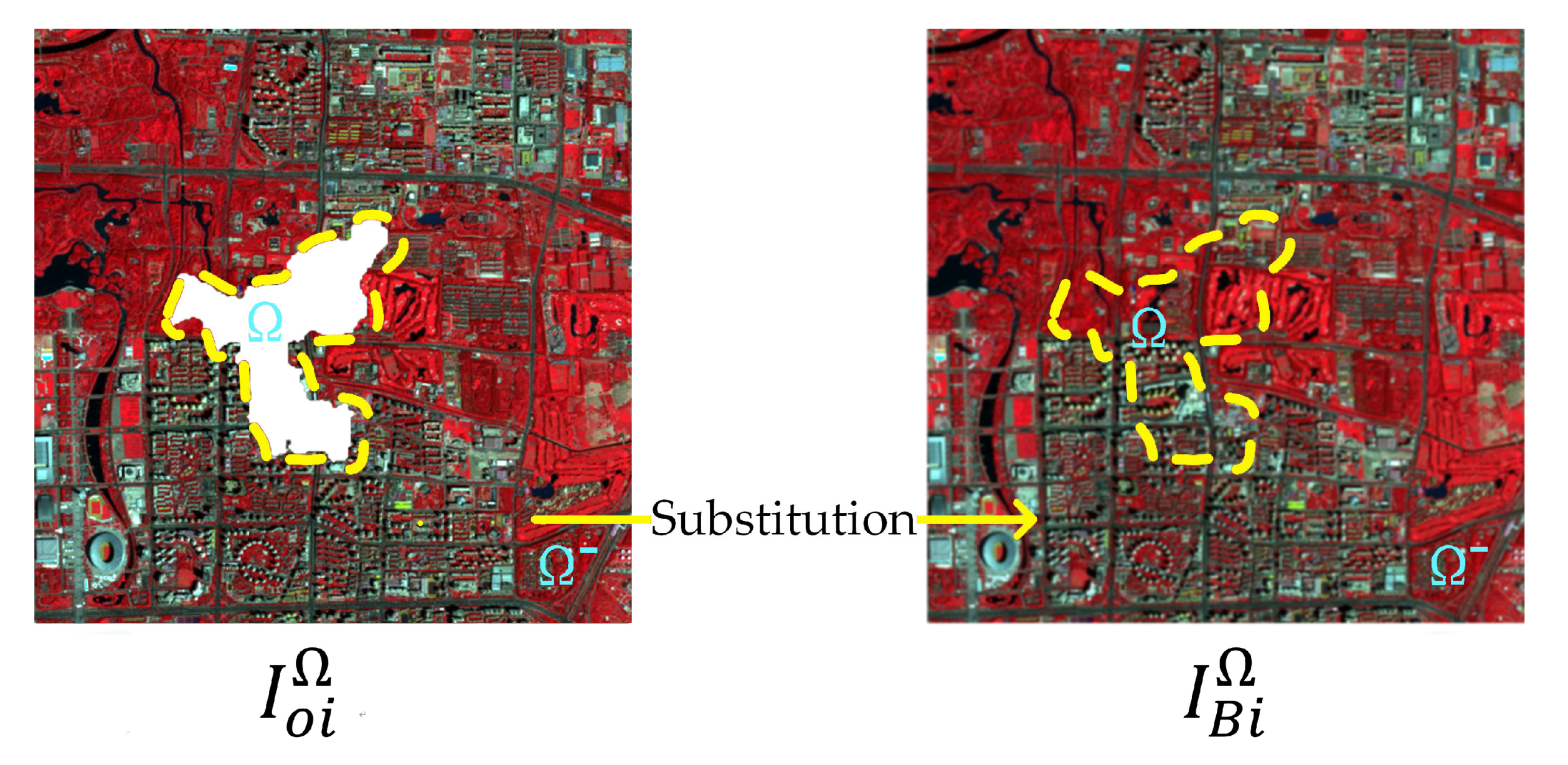
As the sparse representation-based methods process the whole image at the same time, the pixel in the original clear area can be changed, which affects the subsequent processes and application. To address this problem, the clean area in the original cloud-contaminated images is used to fill the corresponding area of the preliminary results. As shown in Figure 6, to facilitate understanding, $I_{oi}$ is used to denote the original cloud-contaminated image in $i$th time node, and $I_{Bi}$ denotes the corresponding image derived from tensor $\mathcal{B}$. The pixels in $I_{Bi}^{{\mathsf{\Omega }}^{-}}$ are replaced by $I_{oi}^{{\mathsf{\Omega }}^{-}}$. The substitution can be represented as

$$I_{Bi}^{{\mathsf{\Omega }}^{-}}= I_{oi}^{{\mathsf{\Omega }}^{-}}$$

(22)

For convenience, the procedure of tensor optimization followed by substitution is called TOS.

2.3. Details Reconstruction

After restoring the cloud/shadow area preliminarily and replacing the original cloud-free area, the detailed information of the cloud/shadow area is reconstructed by information cloning. The image that is closest in the time dimension and that is clean in the corresponding area is taken as the reference image. Inspired by the conception of Poisson editing [42], the problem is modelled as a Poisson equation. To make it easier to explain, $M^{\prime }$ is used to denote the reference image, and $M$ indicates the result of TOS. Let $\mathsf{\Omega }$ represent the recovery area in $M$, and the boundary of $\mathsf{\Omega }$ is denoted as $\partial \mathsf{\Omega }$. The intensity function $f$ to be calculated is defined over the recovery region $\mathsf{\Omega }$, and $f^{\prime }$ denotes the intensity function defined over $M$ minus $\mathsf{\Omega }$. The guidance vector field defined over $\mathsf{\Omega }$ is denoted as $W$. $W$ is defined as the mixing gradients of recovery area in preliminary result and reference image. The problem of reconstructing the optimized result can be formulated as an optimization problem with the boundary condition $f|{ }_{\partial \mathsf{\Omega }}=f^{\prime }|{ }_{\partial \mathsf{\Omega }}$:

$$\underset{f}{\min }\underset{\mathsf{\Omega }}{{\displaystyle \iint }}{\left|\nabla f-W\right|}^2, \mathrm{with} f|{ }_{\partial \mathsf{\Omega }}=f^{\prime }|{ }_{\partial \mathsf{\Omega }}$$

(23)

where $\nabla$ represents the gradient operator, which can be calculated as follows.

$$\begin{gathered} \frac{\partial f\left(x,y\right)}{\partial x}=f\left(x+1,y\right)-f\left(x,y\right) \\ \frac{\partial f\left(x,y\right)}{\partial y}=f\left(x,y+1\right)-f\left(x,y\right) \\ \nabla = \left(\left(\partial /\partial x\right),\left(\partial /\partial y\right)\right) \end{gathered}$$

(24)

Equation (23) devotes to deriving the $f$ with a gradient which is approach $W$ as much as possible, which can be solved as a Poisson equation with Dirichlet boundary condition,

$$\Delta f=div W \mathrm{over} \mathsf{\Omega }, \mathrm{with} f|{ }_{\partial \mathsf{\Omega }}=f^{\prime }|{ }_{\partial \mathsf{\Omega }}$$

(25)

where $div W$ represents the divergence of the vector field $W$, $\Delta$ represents the Laplacian operator, which is defined as $\Delta$= $\left(\raisebox{1ex}{${\partial }^2$}\!\left/ \!\raisebox{-1ex}{$\partial x^2$}\right.\right)+\left(\raisebox{1ex}{${\partial }^2$}\!\left/ \!\raisebox{-1ex}{$\partial y^2$}\right.\right)$

$$\begin{gathered} \frac{{\partial }^{2}f\left(x,y\right)}{\partial x^2} = f\left(x+1,y\right)+f\left(x-1,y\right)-2f\left(x,y\right) \\ \frac{{\partial }^{2}f\left(x,y\right)}{\partial y^2} = f\left(x,y+1\right)+f\left(x,y-1\right)-2f\left(x,y\right) \end{gathered}$$

(26)

where $\left(x,y\right)$ represents the position of the pixel in the image.

The essential formulary of information cloning is shown in Equations (23) and (25), which is an optimization problem constrained by the boundary condition. The boundary condition enforces the consistency of the boundary by constraint formulation $f|{ }_{\partial \mathsf{\Omega }}=f^{\prime }|{ }_{\partial \mathsf{\Omega }}$. Minimization of the ${\ell }^2$ norm represents that the target gradient should be as close as the guidance gradient field. By solving this problem, a seamless cloud/shadow-free image can be obtained.

Equations (23) and (25) can be discretized using the pixel grid. The 4-neighborhood of the pixel $p$ in $M$ is represented as $N_p$, and one of the pixels in 4-neighborhood is represented as $q$. $f\left(p\right)$ denotes the intensity function value at pixel $p$. The aim is to calculate the pixel intensities in $\mathsf{\Omega }$. Equation (23) can be rewritten as the following discrete form:

$$\underset{f}{\min }{{\displaystyle \sum }}_{\langle p,q\rangle {\displaystyle \cap }\mathsf{\Omega }\ne 0}{\left(f\left(p\right)-f\left(q\right)-w_{pq}\right)}^2, \mathrm{with} f\left(p\right)=f^{\prime }\left(p\right) \mathrm{for} \mathrm{all} p\in \partial \mathsf{\Omega }$$

(27)

where $w_{pq}=M^{\prime }\left(p\right)-M^{\prime }\left(q\right)$ denotes the directional gradient of $M$ at pixel $p$.

According to (27), the following equation can be obtained:

$$\left|N_p\right|f\left(p\right)-{\displaystyle \sum }_{q\in N_p{\displaystyle \cap }\mathsf{\Omega }}f\left(q\right)={\displaystyle \sum }_{q\in N_p{\displaystyle \cap }\partial \mathsf{\Omega }}{f}^{\prime }\left(q\right)+{\displaystyle \sum }_{q\in N_p}{w}_{pq} \mathrm{for} \mathrm{all} p\in \mathsf{\Omega }$$

(28)

where $\left|N_p\right|$ is the number of neighbors in $N_p$. The above equation can be solved iteratively until $f$ is converged.

When pixels $p$ is in $\mathsf{\Omega }$ and $N_p\in \mathsf{\Omega }$, there are no boundary terms in the right side of Equation (28)

$$\left|N_p\right|f\left(p\right)-{\displaystyle \sum }_{q\in N_p}f\left(q\right)={\displaystyle \sum }_{q\in N_p}{w}_{pq}$$

(29)

As the general spectral information of the image is recovered in M, it is required to combine the properties of $f^{\prime }$ and the reference image. Therefore, the guidance field should be as follows

$$w\left(s\right)=\{\begin{array}{c}\nabla f^{\prime }\left(s\right) if \left|\nabla f^{\prime }\left(s\right)\right|>\left|\nabla r\left(s\right)\right|,\hfill \\ \nabla r\left(s\right) \mathrm{otherwise}\hfill \end{array} \mathrm{for} \mathrm{all} s\in \mathsf{\Omega }$$

(30)

where $r$ denotes the reference image, and $s$ indicates a pixel in $\mathsf{\Omega }$.

As information cloning uses pixel gradient instead of pixel intensity to process the image, the recovery area looks more realistic.

3. Experimental Results and Analyses

In this part, five groups of experiments that include three simulated experiments and two real-data experiments are conducted on different satellite images with different resolutions and different land features. To verify the performance of the proposed TSSTO method from various aspects, the results of TSSTO are compared with those of the common tensor completion method, FaLRTC and HaLRTC [13], the RPCA-based method TRPCA [27], and the state-of-the-art TVLRSDC [37].

For simulated experiments, the cloud area is simulated on the original clean images. The results of the methods are compared with the original clear images from both visual effect and quantitative assessment. To evaluate the performance of TSSTO for cloud removal in simulated experiments, peak signal-to-noise ratio (PSNR), structural similarity (SSIM) index [43], multiscale structural similarity (MS-SSIM) [44], information content weighted structural similarity (IW-SSIM) [45], figure definition (FD), cross-entropy (CE), and correlation coefficient (CC) index are employed. The simulated experiments and quantitative metrics are introduced in Section 3.1.

For real-data experiments, two datasets covered with real cloud/shadow from different sensors are used to test the performance of TSSTO on real cloud-contaminated images. Since there is no original cloud-free image in the real-data experiments, only no-reference image quality assessments can be used for analysis. Figure definition (FD), standard deviation (SD), information entropy (IE), blind image quality measure of enhanced images (BIQME) [46], and From Patches to Pictures (PaQ-2-PiQ) model [47] are exploited to evaluate the proposed TSSTO method quantitatively. Finally, cloud/shadow detection results are presented and compared to analyze TSSTO further.

3.1. Simulated Experiments

In this part, the cloud areas in different shapes and sizes are simulated on the original clean images that are from different sensors and with different resolutions. Experiments on three groups of simulated cloud-contaminated images are designed to evaluate the effectiveness of the proposed TSSTO method and its sensitivity to cloud size. PSNR, SSIM, MS-SSIM, IW-SSIM, FD, and CE are calculated in the whole image within all bands used in the experiment. Unlike these indexes, CC index is computed between the constructed area and the corresponding area in the original clear image. Following, the quantitative metrics used in simulated experiments are illustrated briefly.

PSNR indicates the ratio of the maximum pixel intensity to the power of the distortion. FD refers to the definition of the images, which is represented by the average gradient of the image. The average gradient reflects the rate of the intensity change in the image of small details. Let $O\left(i,j\right)$ and $R\left(i,j\right)$ denote the $\left(i,j\right)$th pixel in the original clean image and the cloud removal result, respectively. $m$ and $n$ are the numbers of rows and columns in image. PSNR and FD can be defined as Equations (31) and (32), where $MAX$ represents the possible maximum value of all the pixels in image R.

The SSIM metric is a rich synthesis score of luminance, local image structure, and contrast. In SSIM, structures are modes of pixel intensities, peculiarly among neighboring pixels, after normalizing for luminance and contrast. As the human eyes are skilled at perceiving structure, the SSIM quality metric agrees more closely with the subjective quality score than PSNR. The MS-SSIM metric expands on the SSIM index by compounding luminance information at the highest resolution level with structure and contrast information at several downsampled resolutions, or scales. IW-SSIM is an extension of the SSIM by incorporating the idea of information content weighted pooling. The more similar two images are, the larger SSIM, MS-SSIM, and IW-SSIM will achieve.

CE is a popular measure to evaluate the degree of difference between the two images, and lower CE means the result is closer to the original clear image. Equation (33) shows the computation of CE, in which the $g$ is the pixel value, $R\left(g\right)$ and $O\left(g\right)$ are the probability of $g$ in image $R$ and $O$. CC indicates the consistency between the groups of data. Let C denote the total number of the cloud-contaminated pixels. $R_k^c$ and $O_k^c$ are the kth reconstructed pixel value and kth original pixel value of contaminated cloud pixels. $MEA{N}_{RC}$ and $MEA{N}_{OC}$ are the mean values. Specifically, CC can be defined as Equation (34).

The quantitative metrics used in simulated experiments are summarized in

Table 1. The induction of the quantitative metrics used in simulated experiments.

Index	Full Name	Formula or Reference	Note
PSNR	Peak signal-to-noise ratio	Equation (31)	The higher the better
SSIM	Structural similarity index	(Wang et al., 2004) [43]	The higher the better
MS-SSIM	Multiscale structural similarity	(Wang et al., 2003) [44]	The higher the better
IW-SSIM	Information content weighted structural similarity	(Wang et al., 2011) [45]	The higher the better
FD	Figure definition	Equation (32)	The higher the better
CE	Cross-entropy	Equation (33)	The lower the better
CC	Correlation coefficient index	Equation (34)	The higher the better

.

$$\begin{gathered} PSNR=10\times lo{g}_{10}\left(\frac{MAX}{MSE}\right)=20\times lo{g}_{10}\left(\frac{MAX}{\sqrt{MSE}}\right) \\ MSE=\frac{1}{mn}{\displaystyle \sum }_{i=1}^m{\displaystyle \sum }_{j=1}^n{\left[R\left(i,j\right)-O\left(i,j\right)\right]}^2 \end{gathered}$$

(31)

$$FD=\frac{1}{mn}{\displaystyle \sum }_{i=1}^m{\displaystyle \sum }_{j=1}^n\sqrt{\left\{{\left[R\left(i,j\right)-R\left(i,j+1\right)\right]}^2+{\left[R\left(i,j\right)-R\left(i+1,j\right)\right]}^2\right\}/2}$$

(32)

$$CE={\displaystyle \sum }_{g=0}^{MAX-1}R\left(g\right)\frac{{\log }_{2}R\left(g\right)}{O\left(g\right)}$$

(33)

$$CC=\frac{{{\displaystyle \sum }}_{k=1}^{\mathrm{C}}\left(R_k^c-MEA{N}_{RC}\right)\left(O_k^c-MEA{N}_{OC}\right)}{\sqrt{{{\displaystyle \sum }}_{k=1}^{\mathrm{C}}{\left(R_k^c-MEA{N}_{RC}\right)}^2{{\displaystyle \sum }}_{k=1}^{\mathrm{C}}{\left(O_k^c-MEA{N}_{OC}\right)}^2}}$$

(34)

3.1.1. Effectiveness of the Proposed TSSTO Method

In this section, experiments are performed on datasets from Gaofen-1 WFV images, and SPOT-5 images, respectively. The results of the proposed TSSTO method are compared with those of FaLRTC, HaLRTC, TRPCA, and TVLRSDC in both qualitative and quantitative ways.

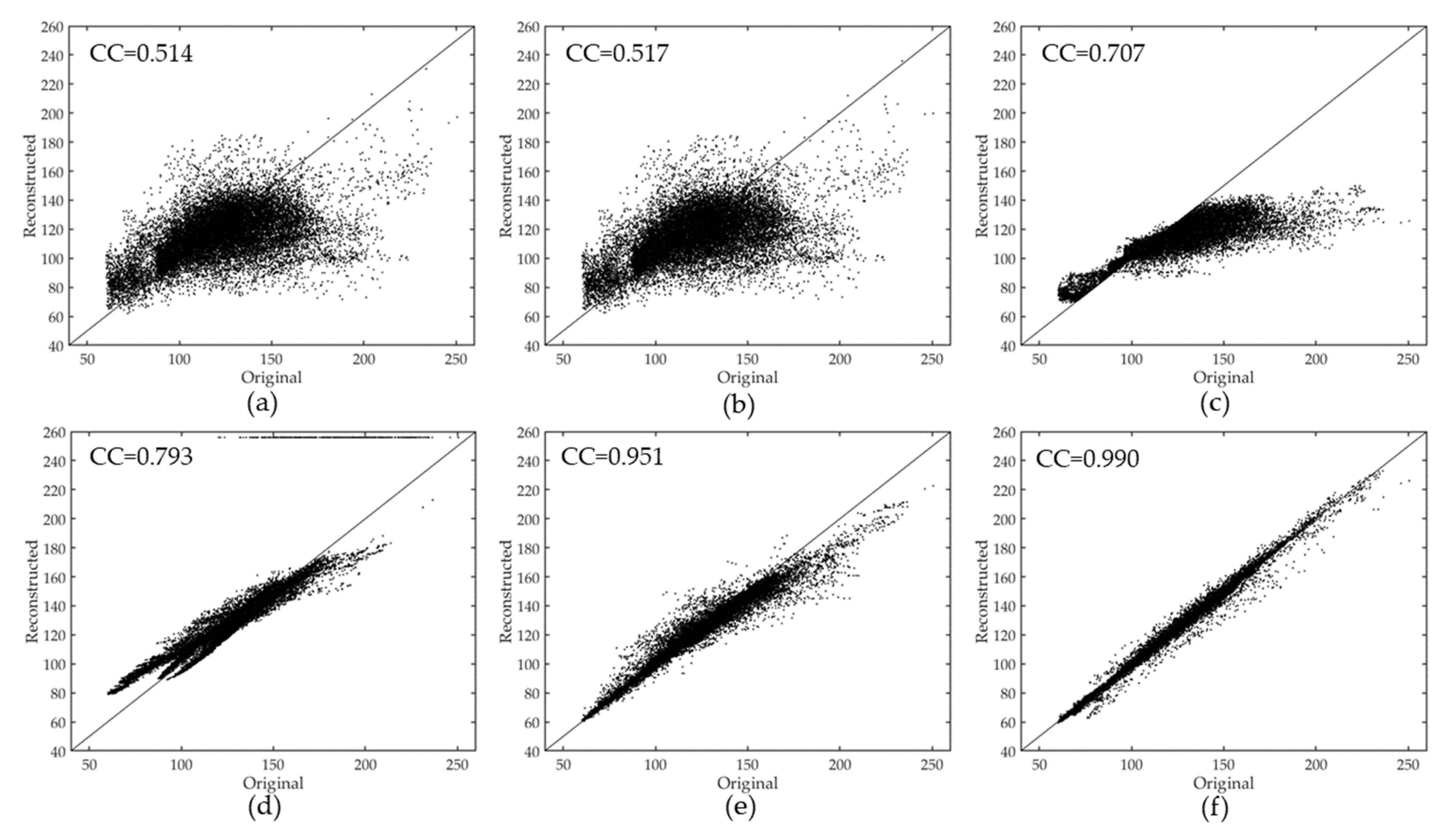
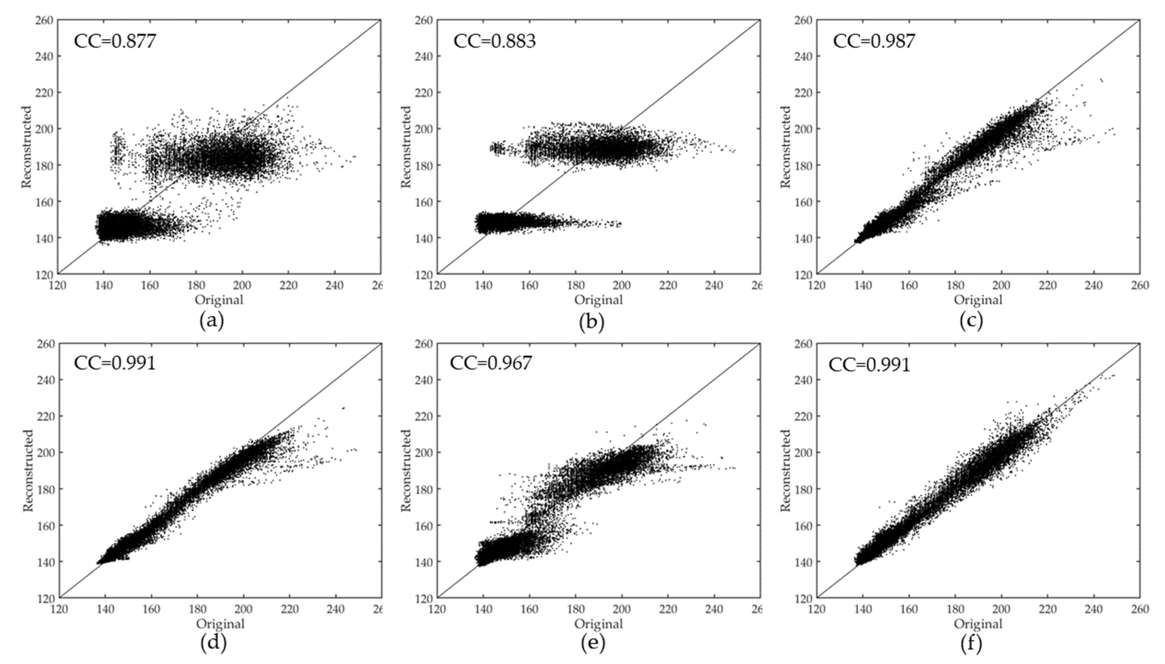
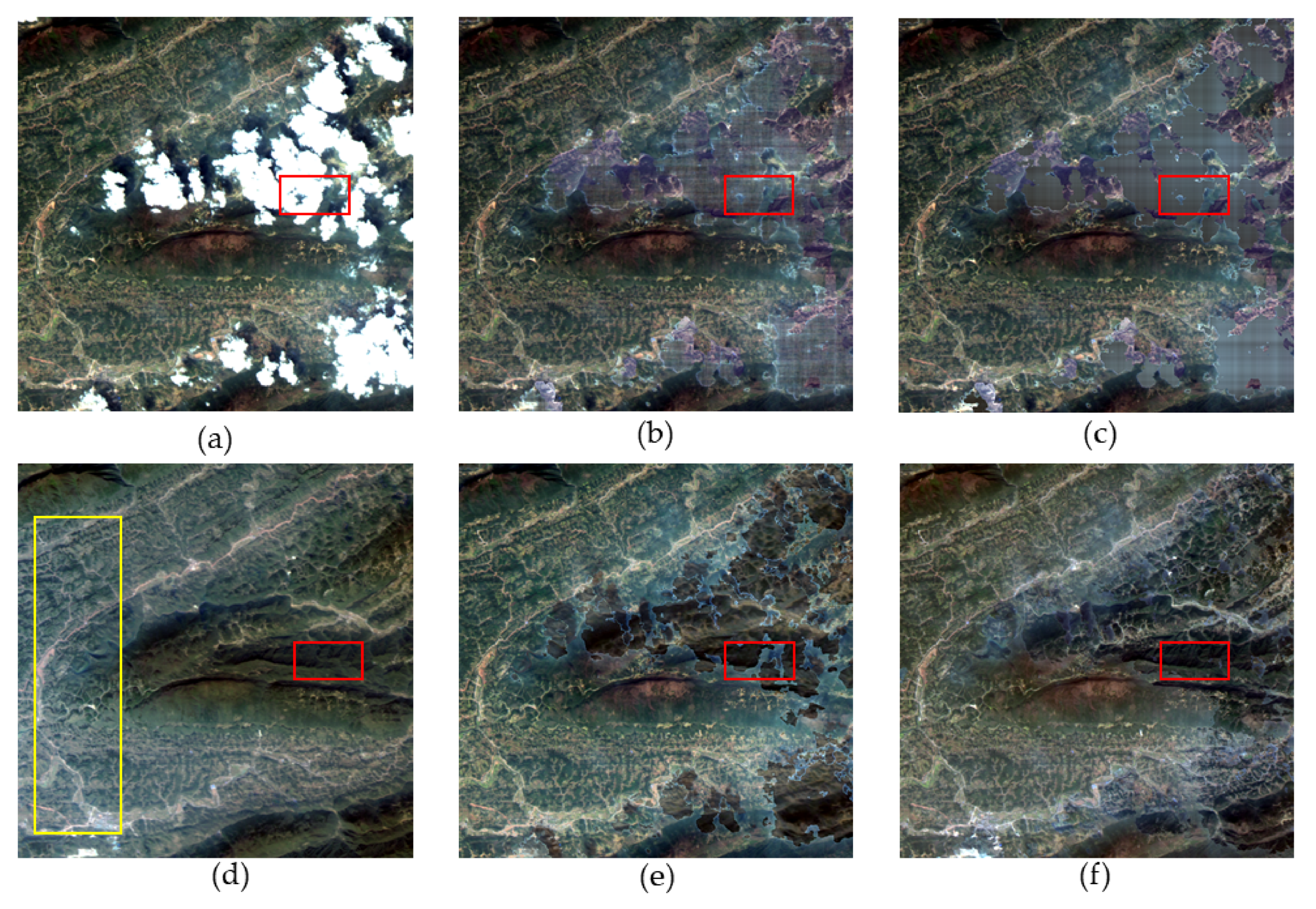
The first simulated experiment is conducted on six Gaofen-1 Wide Field View Multispectral (WFV) images with a size of 512 $\times$ 512 pixels, three bands (bands 1, 2, and 3) of which are used to undertake the test. The images mainly contain the urban area and vegetation, and the images are acquired in October 2015 and December 2015, in Hubei. The original and simulated images of true color composition (red: band 3; green: band 2; blue: band 1) are shown in Figure 7a,b. The recovery results of FaLRTC, HaLRTC, TRPCA, TVLRSDC, TOS, and the proposed TSSTO method are presented in Figure 7c–h. The zoomed detailed regions of images in Figure 7 is shown in Figure 8. The quantitative metrics of the above methods are listed in

Table 2. The PSNR, SSIM, MS-SSIM, IW-SSIM, FD, and CE of the first simulated experimental results. The values of the highest accuracies are in bold.

Index	FaLRTC	HaLRTC	TRPCA	TVLRSDC	TOS	TSSTO
PSNR	35.80	35.83	24.27	46.29	47.25	55.84
SSIM	0.9714	0.9716	0.6936	0.9982	0.9956	0.9998
MS-SSIM	0.9797	0.9797	0.8568	0.9996	0.9990	0.9998
IW-SSIM	0.9631	0.9633	0.9321	0.9996	0.9983	0.9998
FD	1204.27	1204.36	671.69	1213.5	1205.14	1220.96
CE	5.04 × 10−4	2.80 × 10−4	3.98 × 10−1	5.55 × 10−5	9.20 × 10−5	3.37 × 10−5

. The scatterplots with CC for different results are shown in Figure 9.

It can be seen that the ground features are complex, and the details are rich in these images. There is a huge difference between the result of TRPCA (Figure 7e) and the original image (Figure 7a), especially the city area in the bottom left. The reason is that TRPCA changes the values of the pixels in the cloud-free area. For the HaLRTC method, as shown in Figure 7d and Figure 8d, it is evident that the texture information of the result is lost, since no auxiliary information out of the image is used to reconstruct the cloud area. For FaLRTC, some details are lost in the result which does not achieve satisfactory performance, as FaLRTC utilizes no reference images. The result of TVLRSDC (Figure 8f) looks more like the original image than those of the above three contrast methods (Figure 8c–e). The ground features are recovered generally, and the spectral consistency is maintained nicely. In Figure 8, compared to the result of TVLRSDC, the result of TSSTO not only achieves spectral consistency with the original image but also restores more details. The texture in the yellow rectangle in Figure 8h is more refined than the same area in Figure 8f, and the quantitative indexes (Table 2) of the result of TSSTO achieve optimal among all the methods. In addition, the result of TOS restored spectral characteristics generally, which shows the reliability of the proposed model that uses UTV regularizer to constraint the temporal smoothness of the clean element. As shown in Figure 9, the CC values of the HaLRTC and FaLRTC results are no more than 0.6, which are unsatisfactory; CC of the TRPCA and TVLRSDC results are 0.707 and 0.793, respectively, which have a moderate increase; and the result of the proposed TSSTO method gives the highest value of 0.990. These results suggest that the cloud removal results from the proposed TSSTO method can deliver a high-caliber reconstruction result and provide a better support for further applications.

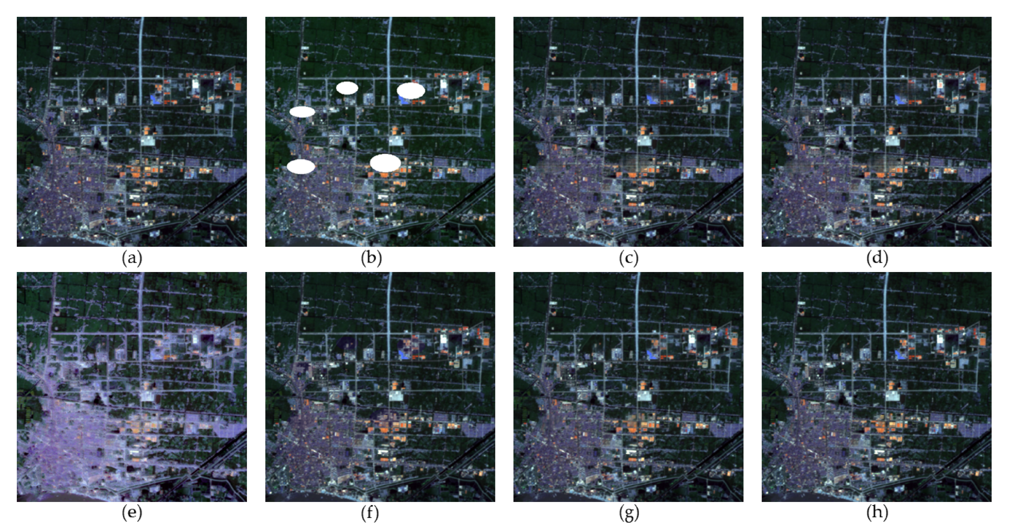
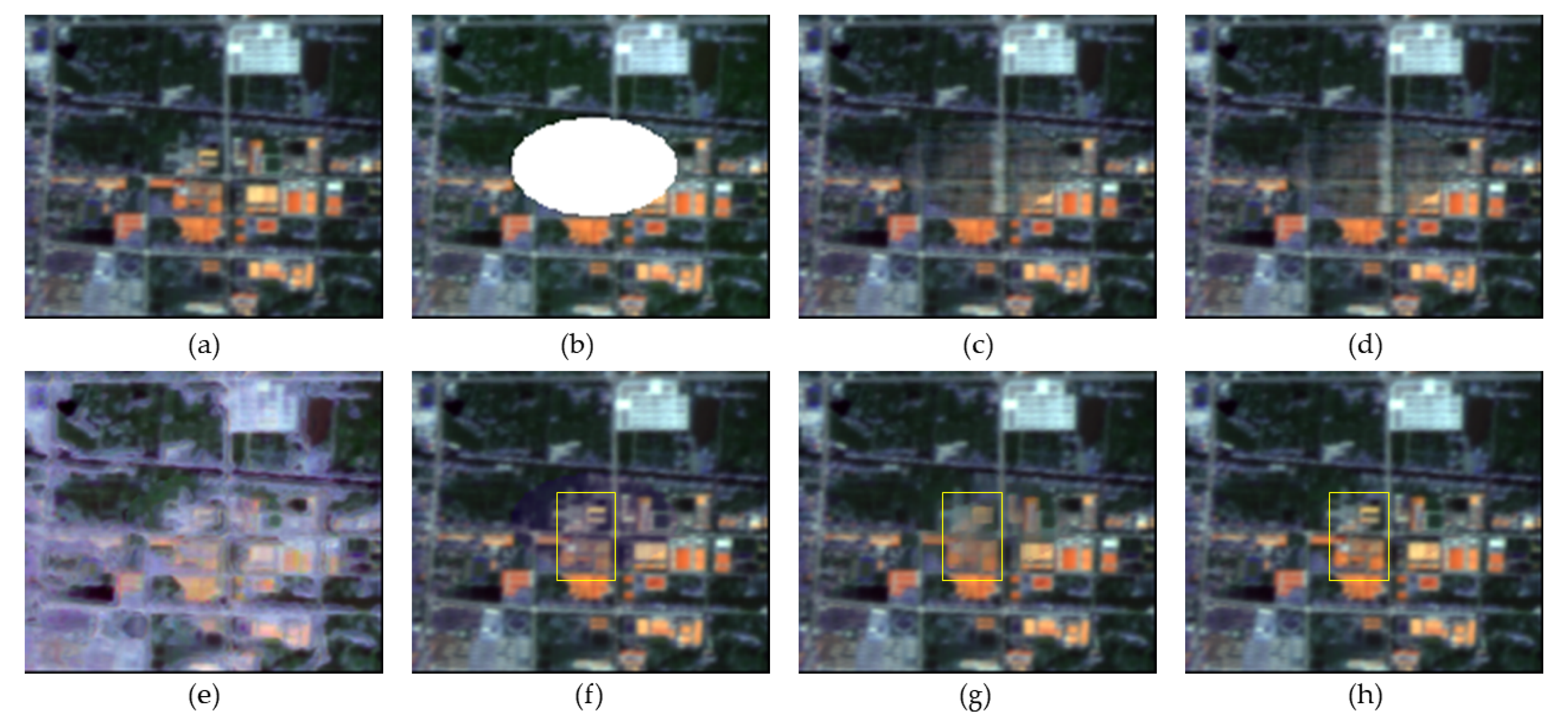
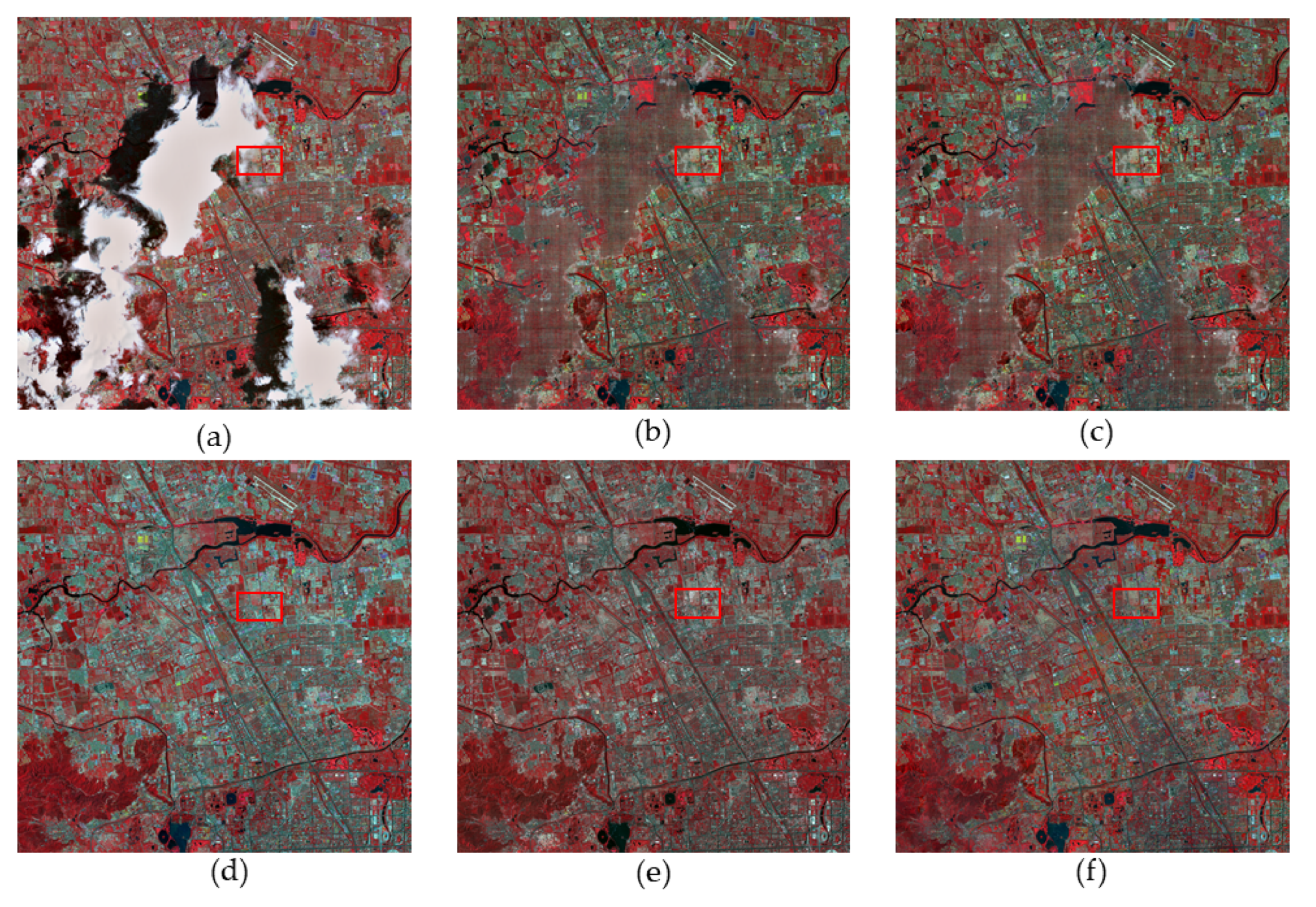
In the second simulated experiment, the proposed TSSTO method is tested on eight SPOT-5 images with four bands (bands 1, 2, 3, and 4) which were acquired in 2015, in Beijing. The size of the experimental images is 512 $\times$ 512 pixels. The original images of false-color composition (red: band 3; green: band 2; blue: band 1) are shown in Figure 10a. The results of the different methods are shown in Figure 10c–h. Figure 11a–h shows the zoomed regions cropped from Figure 10a–h. The quantitative assessment indexes of the above methods were calculated within four bands and listed in

Table 3. The PSNR, SSIM, MS-SSIM, IW-SSIM, FD, and CE of the second simulated experimental results. The values of the highest accuracies are in bold.

Index	FaLRTC	HaLRTC	TRPCA	TVLRSDC	TOS	TSSTO
PSNR	43.20	43.42	36.30	49.98	47.75	52.25
SSIM	0.9644	0.9634	0.9010	0.9976	0.9943	0.9989
MS-SSIM	0.9758	0.9750	0.9635	0.9866	0.9829	0.9890
IW-SSIM	0.9571	0.9583	0.9591	0.9836	0.9788	0.9871
FD	1153.77	1144.97	940.56	1159.46	1148.95	1171.05
CE	3.24 × 10−4	1.55 × 10−3	6.45 × 10−2	8.59 × 10−5	2.84 × 10−4	8.09 × 10−5

. Figure 11 lists the scatterplots with CC for different results.

For the results of FaLRTC (Figure 11c) and HaLRTC (Figure 11d), the reason for the blurry resulting images is that restoring a large amount of texture and structure information is hard just by using little information from the cloud-free part of the image to be repaired. From Table 3, the result of TRPCA gets the unsatisfactory value of metrics, due to the differences in the non-cloud area between the original image and the resulting image (e.g., the area in the yellow rectangle in Figure 10e). In the result of TVLRSDC (Figure 11f), the recovery region looks darker than the rest of the image. This phenomenon may result from that TVLRSDC reshapes the original fourth-order dataset $\mathcal{A}\in$ ${\mathbb{R}}^{m\times n\times b\times t}$ into a matrix $\in$ ${\mathbb{R}}^{mn\times bt}$, which leads to equal treatment of information from the spectral domain and temporal domain. Moreover, with matrix decomposition denoising image and removing cloud, images can be smooth and vague, but there is no processing in the TVLRSDC method to recover the details. For the result of TOS, the values of PSNR, SSIM, MS-SSIM, IW-SSIM, and FD are greater than the results of FaLRTC, HaLRTC, and TRPCA. The reconstructed result of TSSTO is more persuasive with enough details. As shown in Table 3, the quantitative assessments of TSSTO expound the validity of the proposed method as well. In Figure 12, the result of TSSTO is convincing with highest CC.

3.1.2. Sensitivity to Cloud Size

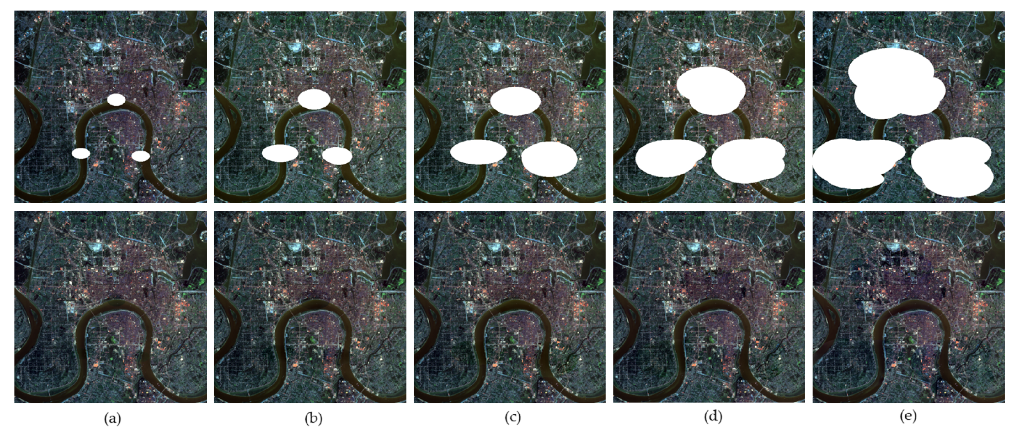
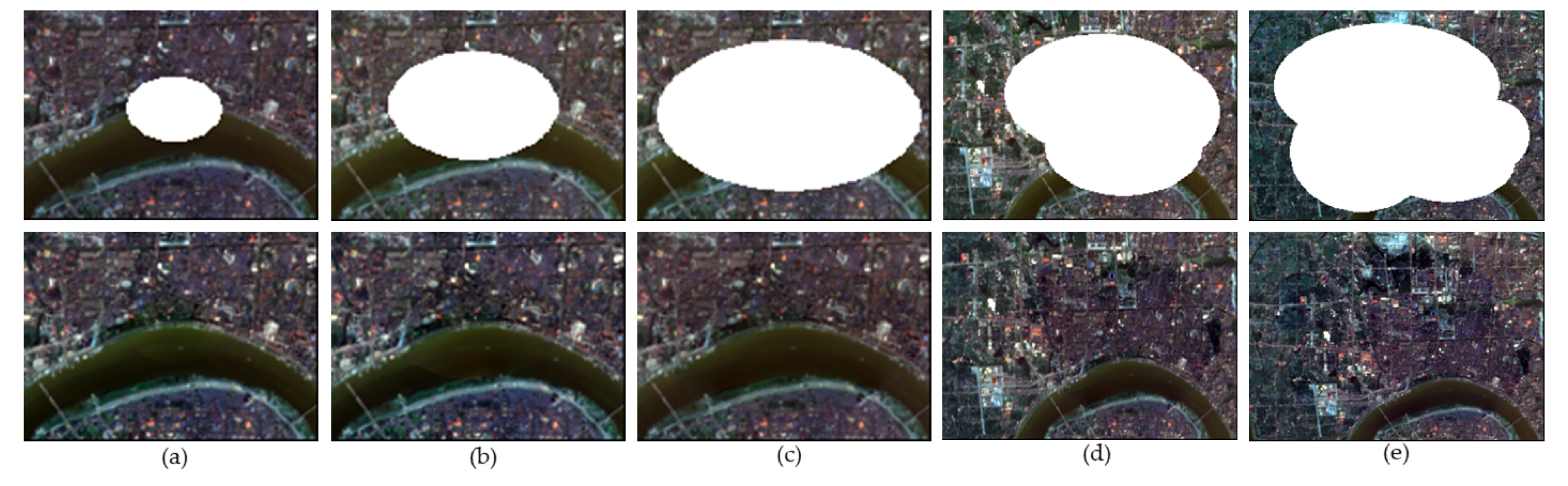
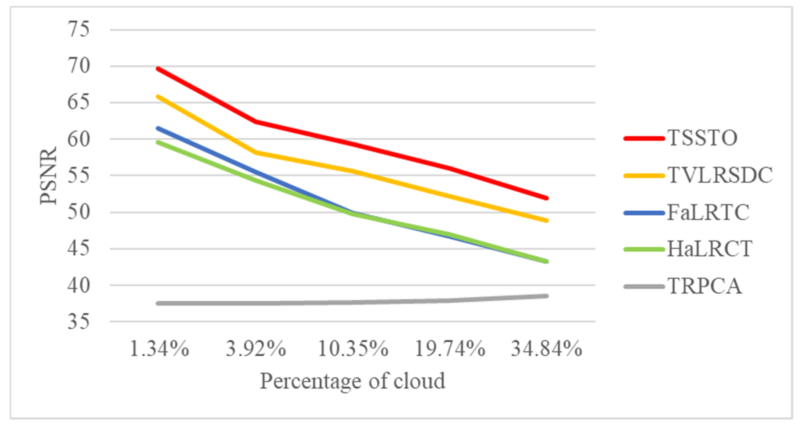
In this section, the insensitivity of the proposed method to the cloud size is proved. The experiment was carried out on 11 well-aligned Landsat-8 OLI images with a size of 512 $\times 512$ pixels, three bands (bands 2, 3, and 4) of which were used to conduct the test, with different sizes of cloud area. With true color composition (red: band 4; green: band 3; blue: band 2), the simulated images and results of TSSTO are shown in Figure 13a,b. The proportions of cloud pixels in the simulated images are 1.34% in Figure 13a, 3.92% in Figure 13b, 10.35% in Figure 13c, 19.74% in Figure 13d, 34.84% in Figure 13e, respectively. The simulated images with the results of different cloud sizes are shown in Figure 13. The zoomed details region of Figure 13 is shown in Figure 14. Figure 15 shows the PSNR values of the results with different methods and cloud sizes.

Figure 13, Figure 14 and Figure 15 can be analyzed as follows. First, since HaLRTC and FaLRTC both reconstruct the cloud-contaminated pixel using information from the cloud-free area of the target image, the curves of PSNR values of HaLRTC and FaLRTC are similar. Second, the proposed TSSTO method can achieve excellent results for cloud removal. As shown in Figure 14e, the proposed TSSTO method can obtain detail-rich and seamless results of cloud removal, even the proportion of cloud in the test image reaches about 35%. Third, although the PSNR value declines with the increasing of the cloud sizes, PSNR values of TSSTO are always more prominent than those of the compared methods. Fourthly, as shown in Figure 15, it is distinct that the performance of TRPCA is barely satisfactory, which can be explained as follows: HaLRTC, FaLRTC, TVLRSDC, and TSSTO change the pixel values in the cloud-contaminated area only, but TRPCA manipulates the cloud-free pixels twice and introduces errors into the cloud-free area. Through the above experiments and analyses, the insensitivity of TSSTO to cloud size is proved. With two sparsity norms regularizers along the horizontal direction and vertical direction applied on cloud/shadow, TSSTO can obtain satisfactory results regardless of the size of the cloud area.

3.2. Real-Data Experiments

In this section, two groups of real-data experiments are conducted on different real cloud-contaminated images from different sensors, and the cloud areas are in different shapes and different sizes. To evaluate the cloud removal results quantitatively, the FD, SD, IE, BIQME, and PaQ-2-PiQ were calculated and listed. These assessments were calculated in the whole image. To make a comprehensive evaluation of the proposed TSSTO method, the cloud/shadow detection results are provided and compared with those of TRPCA and TVLRSDC.

The assessments used to evaluate the results are described below. SD is the simplest way to evaluate image quality, which represents the dispersion degree of pixel value relative to the mean value of the image. Let $R\left(i,j\right)$ denote the $\left(i,j\right)$th pixel in the result, and $m$ and $n$ are the numbers of rows and columns in the resulting image. Then Equation (35) defines SD, where the mean value of image $R$ is represented as $MEA{N}_R$. Larger SD indicates a better image with a more dispersed grey level. IE estimates the amount of information in an image from the information theory perspective. The probability of $g$ in image $R$ is signified by $R\left(g\right)$, and Equation (36) shows the computation of IE, where $MAX$ denotes the possible maximum value of all the pixels in image R. BIQME is proposed in [46], which is a comprehensive evaluation index of contrast, sharpness, brightness, colorfulness, and naturalness of images. PAQ-2-PiQ is a deep learning model trained on a sizeable subjective picture quality dataset for blind or no-reference perceptual picture quality prediction. A higher score generally means a higher quality of an image. More details of PAQ-2-PiQ can be seen in [47].

The quantitative metrics used in real-data experiments are summarized in

Table 4. The induction of the quantitative metrics used in real-data experiments.

Index	Full Name	Formula or Reference	Note
FD	Figure definition	Equation (32)	The higher the better
SD	Standard deviation	Equation (35)	The higher the better
IE	Information entropy	Equation (36)	The higher the better
BIQME	Blind image quality measure of enhanced images	(Gu et al., 2018) [46]	The higher the better
PAQ-2-PiQ	From Patches to Pictures model	(Ying et al., 2020) [47]	The higher the better

.

$$SD=\frac{1}{mn}{\displaystyle \sum }_{i=1}^m{\displaystyle \sum }_{j=1}^n{\left[R\left(i,j\right)-MEA{N}_R\right]}^2$$

(35)

$$IE=-{\displaystyle \sum }_g^{MAX}R\left(g\right){\log }_{2}R\left(g\right)$$

(36)

3.2.1. Real-Data Experiments Results

The first experiment was performed on five Gaofen-1 WFV images with four bands (bands 1, 2, 3, and 4) in the size of 1000 × 1000 pixels, which were acquired in October 2015 and December 2015, in Hubei. Figure 16a shows the original image (true color composition red: band 3; green: band 2; blue: band 1). Figure 16f shows the recovery results of the proposed TSSTO method, and the results of FaLRTC, HaLRTC, TRPCA, TVLRSDC are listed in Figure 16b–e. Figure 17 shows the zoomed detailed regions of images in Figure 16.

Table 5. The SD, FD, IE, BIQME, and PAQ-2-PiQ of the first real-data experimental results. The values of the highest accuracies are in bold.

Index	FaLRTC	HaLRTC	TRPCA	TVLRSDC	TSSTO
SD	89.9728	89.3110	84.8692	88.3581	88.9597
FD	2044.10	1992.41	959.80	2104.80	2087.41
IE	5.9639	5.8964	5.5484	5.7703	5.9279
BIQME	0.5431	0.5531	0.5565	0.5548	0.5691
PAQ-2-PiQ	62.35886	62.36411	64.06165	68.43037	70.99075

lists the values of SD, FD, IE, BIQME, and PAQ-2-PiQ of the results generated by different methods.

As shown in Figure 16, the results of FaLRTC and HaLRTC are not adequate for the demands, due to the difficulty to restore the missing texture only using the information in the clean area. The cloud-free area (e.g., area in the yellow rectangle) is the result of TRPCA () and looks different from the same area in the original image (Figure 16). For the zoomed detailed result of TVLRSDC (Figure 17e), there is some apparent color deviation in the recovery area, as the information in the spectral domain and the temporal domain is processed together and the details are not especially recovered. The result of TSSTO (Figure 16f) is satisfactory visually, and the zoomed area shows that TSSTO achieves optimal results with clear textures and enough details. In Table 5, compared with the results of contrast methods, the majority of the quantitative metrics values of the result of TSSTO is optimal. The experiment results testify the effectiveness of the proposed model that ensures temporal smoothness between images by UTV regularizer along the temporal direction, and band-by-band processing avoids large spectral differences.

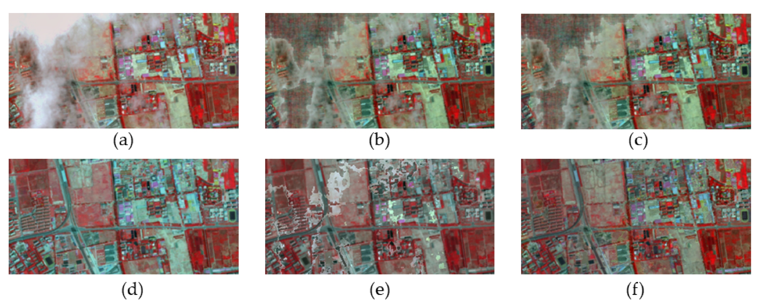
In the second real-data experiment, the proposed TSSTO method was tested on 10 well-aligned SPOT-5 images with a size of 2000 × 2000 pixels. The images were acquired in 2015, in Beijing. Four bands (bands 1, 2, 3, and 4) of the images were used to conduct the test. The original cloud-contaminated image and results of different methods are shown in Figure 18 (red: band 3; green: band 2; blue: band 1). Figure 18a is the original cloud-contaminated image. Figure 18b–f shows the results of FaLRTC, HaLRTC, TRPCA, TVLRDC, and the proposed TSSTO method, respectively. The zoomed detailed regions of images in Figure 18 are represented in Figure 19. The values of quantitative assessments of the results obtained by different methods are listed in

Table 6. The SD, FD, IE, BIQME, and PAQ-2-PiQ of the second real-data experimental results. The values of the highest accuracies are in bold.

Index	FaLRTC	HaLRTC	TRPCA	TVLRSDC	TSSTO
SD	83.2207	82.8479	82.8273	82.1530	83.2207
FD	1275.14	1276.56	1333.00	1259.68	1420.49
IE	7.2976	7.2976	7.3762	7.2784	7.3312
BIQME	73.56364	73.56164	76.84676	77.22347	77.36649
PAQ-2-PiQ	0.5377	0.5265	0.5473	0.5586	0.5620

.

As shown in Figure 18 and Figure 19, the results of FaLRTC and HaLRTC are not acceptable, as large unrepaired area and complex texture information make it difficult to reconstruct the cloud-contaminated area. For the results of TRPCA, TVLRSDC, TSSTO, which are with decent visual effects, it is noticed that the result of TRPCA (Figure 18d) has large spectral differences from the original image (Figure 18a). The transition between the original clean area and the recovery area is not smooth in the result of TVLRDC, as shown in Figure 19e. This deficiency can be explained as follows. There are large differences in the cloud area between the temporal images, while the differences in the cloud area between different bands within a single image are small. Hence, the strategy taken by TVLRSDC that processes the information from the temporal dimension and spectral dimension together can make the result unsatisfactory. Compared with the result of TVLRSDC, the result of TSSTO obtains the refined textures and rich details, as the proposed model guarantees the general spectral information to accord with the cloud-free area and information cloning guarantees fine-grained details in the cloud recovery area.

In this section, to testify the performance of the proposed method, a series of comprehensive experiments were conducted on different datasets. Due to the abundant and various spatial details, the tensor complement method, HaLRTC and FaLRTC cannot reach stable results, in which the reconstructed area appears lack of texture, especially when the cloud area and shadow area contain sophisticated land cover (e.g., river and artificial facilities). TRPCA changes the values of pixels in the original clean area, which makes the result untrustworthy. TVLRSDC can process the information from spectral and temporal domains together. However, the information from different domains is treated equally without discrimination, which may cause abnormal spectral differences. For the proposed TSSTO method, with the recovery of the details in place, the result is optimal in most cases. The visual effect, as well as quantitative indexes, shows that tensor optimization can get the nearly acceptable result and information cloning restore the details effectively.

3.2.2. Cloud/Shadow Detection Result

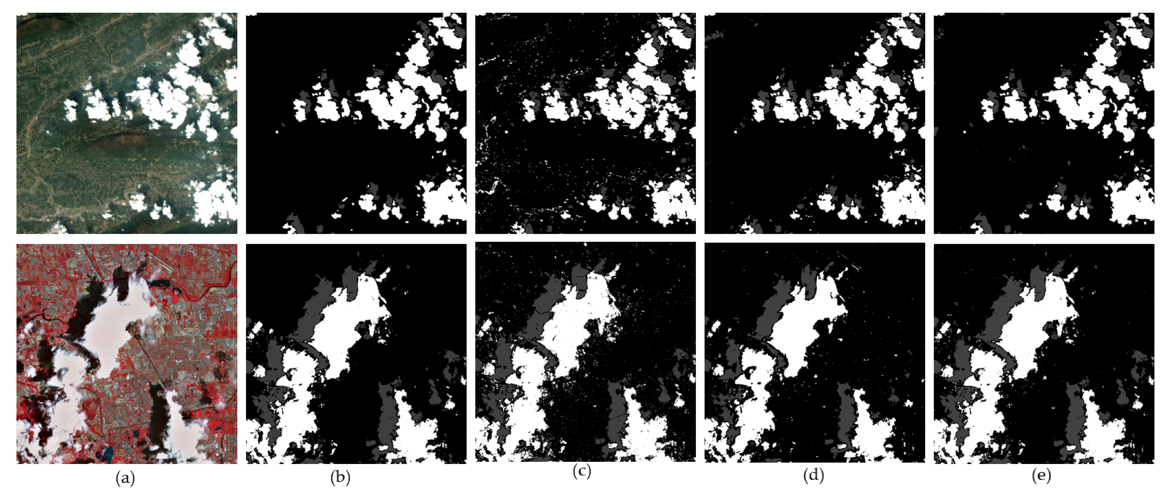
To further evaluate the performance of the proposed TSSTO methods, the cloud/shadow detection results of TRPCA, TVLRSDC, and TSSTO are presented in Figure 20c–e. As there are three categories (cloud, shadow, and clear background) in real-data images to be detected, original images were manually delineated as ground truth (Figure 20b), and overall accuracy (OA), average accuracy (AA), and Kappa coefficient (K) were calculated and displayed in

Table 7. The AA, OA, and Kappa in the real-data experiments. The bold values denote the highest accuracies in each experiment.

Image	Method	OA	AA	$\mathbf{K}\times 100$
Gaofen-1 WFV image	TRPCA	91.28	91.91	87.30
	TVLRSDC	91.72	91.94	88.05
	TSSTO	93.08	93.30	90.92
SPOT-5 image	TRPCA	89.56	78.99	77.93
	TVLRSDC	91.15	82.41	82.91
	TSSTO	92.51	85.80	87.07

to demonstrate the feasibility of the proposed TSSTO. Concretely, OA represents the ratio of the correct classifications of total pixels. AA means the average accuracy of all categories, and the K measures the consistency between the ground truth and detection result. The higher these three metric values are, the better the detection result is.

From Figure 20, cloud/shadow detection results of TSSTO look convincing, according to the original cloud-contaminated images. For Gaofen-1 WFV image, it can be noticed that some cloud-free areas are detected as the cloud by TRPCA, while some cloud-free regions are recognized as the shadow by TVLRSDC. For SPOT-5 image, TSSTO also delivers a more accurate mask, which enables cloud removal methods not to change the pixels in the cloud-free area as much as possible and helps to preserve the spectral characteristics of cloud-free regions. The quantity indexes also demonstrate the effectiveness of the proposed TSSTO, which can be seen in Table 7.

4. Conclusions

This paper proposed a novel TSSTO method for remote sensing images cloud/shadow removal using tensor optimization based on temporal smoothness and sparsity. Specifically, the smoothness along different directions is guaranteed by the UTV regularization terms, and the sparsity is enhanced by the group sparse norm. Furthermore, the convergence of the model is ensured by the ADMM framework in theory. The flow of the proposed TSSTO method encompasses three steps: tensor optimization, the substitution of cloud/shadow-free area, and information cloning. In the tensor optimization step, the cloud/shadow element and the clean element is generated by executing the proposed model. In the substitution step, the cloud/shadow area is determined by the threshold segmentation to obtain the cloud/shadow mask, thereby replacing the original clean area in the preliminary result with the same area of the original image guided by the generated mask. Finally, information cloning is applied to restore more details in the recovery area. A series of experiments have been conducted on the different datasets, which verifies that the proposed TSSTO method not only can recover the cloud area and cloud shadow area with fine-grained details but also can keep spectral consistency and the continuity well. What is more, the increasing size of the cloud areas shows little influence on the proposed method.

Meanwhile, TSSTO still has room for improvement. First, the result of TSSTO is related to the result of cloud/shadow detection, which means the performance of TSSTO leverages on credible cloud/shadow detection result. The authors will make a good effort to study and to overcome this limitation. Second, reliance on the quality of input images reduces some application scenarios of TSSTO. In the future, it is worth making appropriate use of the information that in the spectral domain, spatial domain, and temporal domain jointly weaken the dependency on the quality of the input images and better reconstruct the cloud-contaminated area.

References

- Li, R.; Zheng, S.; Duan, C.; Yang, Y.; Wang, X. Classification of hyperspectral image based on double-branch dual-attention mechanism network. Remote Sens. 2020, 12, 582. [Google Scholar] [CrossRef] [Green Version]
- Amini, S.; Homayouni, S.; Safari, A.; Darvishsefat, A.A. Object-based classification of hyperspectral data using Random Forest algorithm. Geo-Spat. Inf. Sci. 2018, 21, 127–138. [Google Scholar] [CrossRef] [Green Version]
- Yokoya, N.; Iwasaki, A. Object detection based on sparse representation and Hough voting for optical remote sensing imagery. IEEE J. Sel. Top. Appl. Earth Obs. Remote Sens. 2015, 8, 2053–2062. [Google Scholar] [CrossRef]
- Inglada, J.; Vincent, A.; Arias, M.; Tardy, B.; Morin, D.; Rodes, I. Operational high resolution land cover map production at the country scale using satellite image time series. Remote Sens. 2017, 9, 95. [Google Scholar] [CrossRef] [Green Version]
- Li, Z.; Shen, H.; Cheng, Q.; Li, W.; Zhang, L. Thick cloud removal in high-resolution satellite images using stepwise radiometric adjustment and residual correction. Remote Sens. 2019, 11, 1925. [Google Scholar] [CrossRef] [Green Version]
- Rossi, R.E.; Dungan, J.L.; Beck, L.R. Kriging in the shadows: Geostatistical interpolation for remote sensing. Remote Sens. Environ. 1994, 49, 32–40. [Google Scholar] [CrossRef]
- Van der Meer, F. Remote-sensing image analysis and geostatistics. Int. J. Remote Sens. 2012, 33, 5644–5676. [Google Scholar] [CrossRef]
- Criminisi, A.; Pérez, P.; Toyama, K. Region filling and object removal by exemplar-based image inpainting. IEEE Trans. Image Process. 2004, 13, 1200–1212. [Google Scholar] [CrossRef]
- Maalouf, A.; Carré, P.; Augereau, B.; Fernandez-Maloigne, C. A bandelet-based inpainting technique for clouds removal from remotely sensed images. IEEE Trans. Geosci. Remote Sens. 2009, 47, 2363–2371. [Google Scholar] [CrossRef]
- Shen, H.; Zhang, L. A MAP-based algorithm for destriping and inpainting of remotely sensed images. IEEE Trans. Geosci. Remote Sens. 2009, 47, 1490–1500. [Google Scholar]
- Cheng, Q.; Shen, H.; Zhang, L.; Zhang, L.; Peng, Z. Missing information reconstruction for single remote sensing images using structure-preserving global optimization. IEEE Signal Process. Lett. 2017, 24, 1163–1167. [Google Scholar] [CrossRef]
- Zeng, C.; Shen, H.; Zhang, L. Recovering missing pixels for Landsat ETM+ SLC-off imagery using multi-temporal regression analysis and a regularization method. Remote Sens. Environ. 2013, 131, 182–194. [Google Scholar] [CrossRef]
- Liu, J.; Musialski, P.; Wonka, P.; Ye, J. Tensor completion for estimating missing values in visual data. IEEE Trans. Pattern Anal. Mach. Intell. 2013, 35, 208–220. [Google Scholar] [CrossRef] [PubMed]
- Cheng, Q.; Shen, H.; Zhang, L.; Yuan, Q.; Zeng, C. Cloud removal for remotely sensed images by similar pixel replacement guided with a spatio-temporal mrf model. ISPRS J. Photogramm. Remote Sens. 2014, 92, 54–68. [Google Scholar] [CrossRef]
- Rakwatin, P.; Takeuchi, W.; Yasuoka, Y. Restoration of aqua MODIS band 6 using histogram matching and local least squares fitting. IEEE Geosci. Remote Sens. Lett. 2009, 47, 613–627. [Google Scholar] [CrossRef]
- Shen, H.; Zeng, C.; Zhang, L. Recovering reflectance of AQUA MODIS band 6 based on within-class local fitting. IEEE J. Sel. Top. Appl. Earth Observ. Remote Sens. 2011, 4, 185–192. [Google Scholar] [CrossRef]
- Gladkova, I.; Grossberg, M.D.; Shahriar, F.; Bonev, G.; Romanov, P. Quantitative restoration for MODIS band 6 on aqua. IEEE Trans. Geosci. Remote Sens. 2012, 50, 2409–2416. [Google Scholar] [CrossRef]
- Li, H.; Zhang, L.; Shen, H.; Li, P. A variational gradient-based fusion method for visible and SWIR imagery. Photogramm. Eng. Remote Sens. 2012, 78, 947–958. [Google Scholar] [CrossRef]
- Zhang, Y.; Guindon, B.; Cihlar, J. An image transform to characterize and compensate for spatial variations in thin cloud contamination of Landsat images. Remote Sens. Environ. 2002, 82, 173–187. [Google Scholar] [CrossRef]
- Malek, S.; Melgani, F.; Bazi, Y.; Alajlan, N. Reconstructing cloud-contaminated multispectral images with contextualized autoencoder neural networks. IEEE Trans. Geosci. Remote Sens. 2018, 56, 2270–2282. [Google Scholar] [CrossRef]
- Storey, J.; Scaramuzza, P.; Schmidt, G.; Barsi, J. Landsat 7 scan line corrector-off gap-filled product development. In Proceedings of the Pecora 16 Conference on Global Priorities in Land Remote Sensing, Sioux Falls, SD, USA, 23–27 October 2005. [Google Scholar]
- Zhang, X.; Qin, F.; Qin, Y. Study on the thick cloud removal method based on multi-temporal remote sensing images. In Proceedings of the 2010 International Conference on Multimedia Technology, Ningbo, China, 29–31 October 2010; IEEE: Piscataway, NJ, USA; pp. 1–3. [Google Scholar]
- Du, W.; Qin, Z.; Fan, J.; Gao, M.; Wang, F.; Abbasi, B. An efficient approach to remove thick cloud in VNIR bands of multi-temporal remote sensing images. Remote Sens. 2019, 11, 1284. [Google Scholar] [CrossRef] [Green Version]
- Zeng, C.; Long, D.; Shen, H.; Wu, P.; Cui, Y.; Hong, Y. A two-step framework for reconstructing remotely sensed land surface temperatures contaminated by cloud. ISPRS J. Photogramm. Remote Sens. 2018, 141, 30–45. [Google Scholar] [CrossRef]
- Lin, C.H.; Tsai, P.H.; Lai, K.H.; Chen, J.Y. Cloud removal from multitemporal satellite images using information cloning. IEEE Trans. Geosci. Remote Sens. 2012, 51, 232–241. [Google Scholar] [CrossRef]
- Lin, C.H.; Lai, K.H.; Chen, Z.B.; Chen, J.Y. Patch-based information reconstruction of cloud-contaminated multitemporal images. IEEE Trans. Geosci. Remote Sens. 2013, 52, 163–174. [Google Scholar] [CrossRef]
- Wen, F.; Zhang, Y.; Gao, Z.; Ling, X. Two-pass robust component analysis for cloud removal in satellite image sequence. IEEE Geosci. Remote Sens. Lett. 2018, 15, 1090–1094. [Google Scholar] [CrossRef]
- Zhang, Y.; Wen, F.; Gao, Z.; Ling, X. A Coarse-to-Fine Framework for Cloud Removal in Remote Sensing Image Sequence. IEEE Trans. Geosci. Remote Sens. 2019, 57, 5963–5974. [Google Scholar] [CrossRef]
- Li, X.; Shen, H.; Zhang, L.; Zhang, H.; Yuan, Q.; Yang, G. Recovering quantitative remote sensing products contaminated by thick clouds and shadows using multitemporal dictionary learning. IEEE Trans. Geosci. Remote Sens. 2014, 52, 7086–7098. [Google Scholar]
- Li, X.; Shen, H.; Zhang, L.; Li, H. Sparse-based reconstruction of missing information in remote sensing images from spectral/temporal complementary information. ISPRS J. Photogramm. Remote Sens. 2015, 106, 1–15. [Google Scholar] [CrossRef]
- Li, X.; Shen, H.; Li, H.; Zhang, L. Patch matching-based multitemporal group sparse representation for the missing information reconstruction of remote-sensing images. IEEE J. Sel. Top. Appl. Earth Obs. Remote Sens. 2016, 9, 3629–3641. [Google Scholar] [CrossRef]
- Xu, M.; Jia, X.; Pickering, M.; Plaza, A.J. Cloud removal based on sparse representation via multitemporal dictionary learning. IEEE Trans. Geosci. Remote Sens. 2016, 54, 2998–3006. [Google Scholar] [CrossRef]
- Li, X.; Wang, L.; Cheng, Q.; Wu, P.; Gan, W.; Fang, L. Cloud removal in remote sensing images using nonnegative matrix factorization and error correction. ISPRS J. Photogramm. Remote Sens. 2019, 148, 103–113. [Google Scholar] [CrossRef]
- Ng, M.K.P.; Yuan, Q.; Yan, L.; Sun, J. An adaptive weighted tensor completion method for the recovery of remote sensing images with missing data. IEEE Trans. Geosci. Remote Sens. 2017, 55, 3367–3381. [Google Scholar] [CrossRef]
- Cheng, Q.; Yuan, Q.; Ng, M.K.P.; Shen, H.; Zhang, L. Missing Data Reconstruction for Remote Sensing Images with Weighted Low-Rank Tensor Model. IEEE Access 2019, 7, 142339–142352. [Google Scholar] [CrossRef]
- Ji, T.Y.; Yokoya, N.; Zhu, X.X.; Huang, T.Z. Nonlocal tensor completion for multitemporal remotely sensed images’ inpainting. IEEE Trans. Geosci. Remote Sens. 2017, 56, 3047–3061. [Google Scholar] [CrossRef]
- Chen, Y.; He, W.; Yokoya, N.; Huang, T.Z. Blind cloud and cloud shadow removal of multitemporal images based on total variation regularized low-rank sparsity decomposition. ISPRS J. Photogramm. Remote Sens. 2019, 157, 93–107. [Google Scholar] [CrossRef]
- Zhang, Q.; Yuan, Q.; Zeng, C.; Li, X.; Wei, Y. Missing data reconstruction in remote sensing image with a unified spatial-temporal-spectral deep convolutional neural network. IEEE Trans. Geosci. Remote Sens. 2018, 56, 4274–4288. [Google Scholar] [CrossRef] [Green Version]
- Boyd, S.; Parikh, N.; Chu, E.; Peleato, B.; Eckstein, J. Distributed Optimization and Statistical Learning via the Alternating Direction Method of Multipliers. Foundations and Trends in Machine Learning; Now Publishers Inc.: Breda, The Netherlands, 2010; Volume 3, pp. 1–122. [Google Scholar]
- Lin, Z.; Chen, M.; Ma, Y. The augmented Lagrange multiplier method for exact recovery of corrupted low-rank matrices. arXiv 2010, arXiv:1009.5055. [Google Scholar]
- Deng, W.; Yin, W.-T.; Zhang, Y. Group sparse optimization by alternating direction method. In Proceedings of the International Society of Optics and Photonics (SPIE), San Diego, CA, USA, 25–29 August 2013; SPIE: Bellingham, WA, USA, 2013. [Google Scholar]
- Pérez, P.; Gangnet, M.; Blake, A. Poisson image editing. ACM Trans. Graph. 2003, 22, 313–318. [Google Scholar] [CrossRef]
- Wang, Z.; Bovik, A.; Sheikh, H.; Simoncelli, E. Image quality assessment: From error visibility to structural similarity. IEEE Trans. Image Process. 2004, 13, 600–612. [Google Scholar] [CrossRef] [Green Version]
- Wang, Z.; Simoncelli, E.P.; Bovik, A.C. Multi-scale structural similarity for image quality assessment. In Proceedings of the Thirty-Seventh Asilomar Conference on Signals, Systems and Computers 2003, Pacific Grove, CA, USA, 9–12 November 2013; Volume 2, pp. 1398–1402. [Google Scholar]
- Wang, Z.; Li, Q. Information Content Weighting for Perceptual Image Quality Assessment. IEEE Trans. Image Process. 2011, 20, 1185–1198. [Google Scholar] [CrossRef]
- Gu, K.; Tao, D.; Qiao, J.; Lin, W. Learning a No-Reference Quality Assessment Model of Enhanced Images with Big Data. IEEE Trans. Neural Netw. Learn. Syst. 2018, 29, 1301–1313. [Google Scholar] [CrossRef] [PubMed] [Green Version]
- Ying, Z.; Niu, H.; Gupta, P.; Mahajan, D.; Ghadiyaram, D.; Bovik, A. From Patches to Pictures (PaQ-2-PiQ): Mapping the Perceptual Space of Picture Quality. In Proceedings of the 2020 IEEE/CVF Conference on Computer Vision and Pattern Recognition (CVPR), Seattle, WA, USA, 13–19 June 2020. [Google Scholar]
Figure 1.
Flowchart of the proposed Temporal Smoothness and Sparsity-regularized Tensor Optimization (TSSTO) method.
Figure 2.
The images used to draw histograms (a) original cloud-contaminated images; (b) clean element; (c) cloud/shadow element.
Figure 3.
The histogram of the absolute values of the horizontal gradient of (a) cloud/shadow element and (b) clean element.
Figure 4.
The histogram of the absolute values of the vertical gradient of (a) cloud/shadow element and (b) clean element.
Figure 5.
The histogram of the absolute values of the temporal gradient of (a) cloud/shadow element and (b) clean element.
Figure 6.
Explanation of substitution.
Figure 7.
Gaofen-1 WFV images for the first simulated experiment: (a) original clean image; (b) simulated cloud image; (c–h) the results of FaLRTC, HaLRTC, TRPCA, TVLRSDC, TOS, and TSSTO, respectively.
Figure 8.
(a–h) Detailed regions clipped from Figure 7a–h.
Figure 9.
The scatterplots of the original and the reconstructed values in the first simulated experiment: (a) the FaLRTC method; (b) the HaLRTC method; (c) the TRPCA method; (d) the TVLRSDC method; (e) the TOS method; (f) the proposed TSSTO method.
Figure 10.
SPOT-5 images for the second simulated experiment: (a) original clean image; (b) simulated cloud image; (c–h) the results of FaLRTC, HaLRTC, TRPCA, TVLRSDC, TOS, and TSSTO, respectively.
Figure 11.
(a–h) Detailed regions clipped from Figure 10a–h.
Figure 12.
The scatterplots of the original and the reconstructed values in the second simulated experiment: (a) the FaLRTC method; (b) the HaLRTC method; (c) the TRPCA method; (d) the TVLRSDC method; (e) the TOS method; (f) the proposed TSSTO method.
Figure 13.
The simulated images and results with different cloud sizes. The proportions of cloud pixels in the simulated images are 1.34% (a), 3.92% (b), 10.35% (c), 19.74% (d), 34.84% (e), respectively.
Figure 14.
(a–e) Detailed regions clipped from Figure 13a–e.
Figure 15.
The PSNR values of the results with different methods and cloud sizes.
Figure 16.
Gaofen-1 WFV images for the second real-data experiment: (a) cloud image; (b–f) the results of FaLRTC, HaLRTC, TRPCA, TVLRSDC, and TSSTO, respectively.
Figure 17.
(a–f) Detailed regions clipped from Figure 16a–f.
Figure 18.
SPOT-5 images for the third real-data experiment: (a) cloud image; (b–f) the results of FaLRTC, HaLRTC, TRPCA, TVLRSDC, and TSSTO, respectively.
Figure 19.
(a–f) Detailed regions clipped from Figure 18a–f.
Figure 20.
Cloud/shadow detection results for the real-data experiments. (a) Cloud image; (b) ground truth; (c–e) the detection results of TRPCA, TVLRSDC, and TSSTO, respectively.