Quasi-Active Thermal Imaging of Large Floating Covers Using Ambient Solar Energy
by
 , ,
, ,
Yue Ma
1,*, 
Leslie Wong
1,
Benjamin Steven Vien
1,
Thomas Kuen
2,
Jayantha Kodikara
3 and
Wing Kong Chiu
1 1
Department of Mechanical & Aerospace Engineering, Monash University, Clayton VIC 3800, Australia
2
Department of Integrated Planning, Melbourne Water Corporation, 990 La Trobe Street, Docklands, Melbourne VIC 3008, Australia
3
Department of Civil Engineering, Monash University, Clayton VIC 3168, Australia
*
Author to whom correspondence should be addressed.
Remote Sens. 2020, 12(20), 3455; https://0-doi-org.brum.beds.ac.uk/10.3390/rs12203455
Submission received: 28 September 2020
/
Accepted: 19 October 2020
/
Published: 21 October 2020
Abstract
:Melbourne Water Corporation has two large anaerobic lagoons at the Western Treatment Plant (WTP), Werribee, Victoria, Australia. The lagoons are covered using numerous sheets of high-density polyethylene (HDPE) geomembranes to prevent the emission of odorous gases and to harness biogas as a source of renewable energy. Some of the content of raw sewage can accumulate and form into a solid mass (called “scum”). The development of a large body of solid scum that rises to the surface of the lagoon (called “scumbergs”) deforms the covers and may affect its structural integrity. Currently, there is no method able to effectively “see-through” the opaque covers to define the spread of the scum underneath the cover. Hence, this paper investigates a new quasi-active thermal imaging method that uses ambient solar radiation to determine the extent of the solid matter under the geomembrane. This method was devised by using infrared thermography and a pyranometer to constantly monitor the transient temperature response of the HDPE geomembrane using the time varying ambient solar radiation. Newton’s cooling law is implemented to define the resultant cooling constants. The results of laboratory-scale tests demonstrate the capability of the quasi-active thermography to identify the presence and the extent of solid matter under the cover. This paper demonstrates, experimentally, the importance of measuring the surface temperature of the cover and solar intensity profiles to obtain the cooling process when during variations in solar intensity during normal sunrise, sunset, daily transitioning from morning–afternoon–evening and cloud cover events. The timescale associated with these events are different and the results show that these daily transient temperature cycles of the geomembranes can be used to detect the extent of the accumulation of solid matter underneath the geomembrane. The conclusions from this work will be further developed for field trials to practically monitor the growth in the extent of the scum under the floating covers in WTP with the ambient solar energy.

1. Introduction
Melbourne Water Corporation (MWC) owns and operates the self-powered Western Treatment Plant (WTP) at Werribee, Victoria, Australia. The WTP normally treats over half of Melbourne’s sewage (>300 GL per annum) and, hence, delivers a significant and important service to a very large urban area and population. The resource recovery programs at WTP turn the sewage into valuable products including biogas for on-site production of electricity and recycled water for agriculture customers. WTP utilizes the biogas captured from the covered anaerobic lagoons to generate renewable energy to supply all the electricity required to run the site and exports surplus electricity to the grid. The entire sewage treatment process can take up to 40 days in the lagoon systems (up to 10 ponds) before the end products can be reused as recycled water or discharged to the receiving water of Port Philip. At the WTP, the raw sewage (from household waste, high-strength organic waste and waste from meat and dairy food industries) will first pump directly to the first treatment lagoon (a 6 to 8 m deep pond) for the removal of solids. The flow of sewage slows down as it enters these large and deep lagoons, allowing most of the suspended solids in the sewage to sink to the bottom and form a layer of sludge. At the first treatment lagoon, a suitable anaerobic environment is also provided for bacteria to break down the organic material into sludge, releasing biogas (i.e., methane and hydrogen sulfide, H2S) which can be turned into electricity.
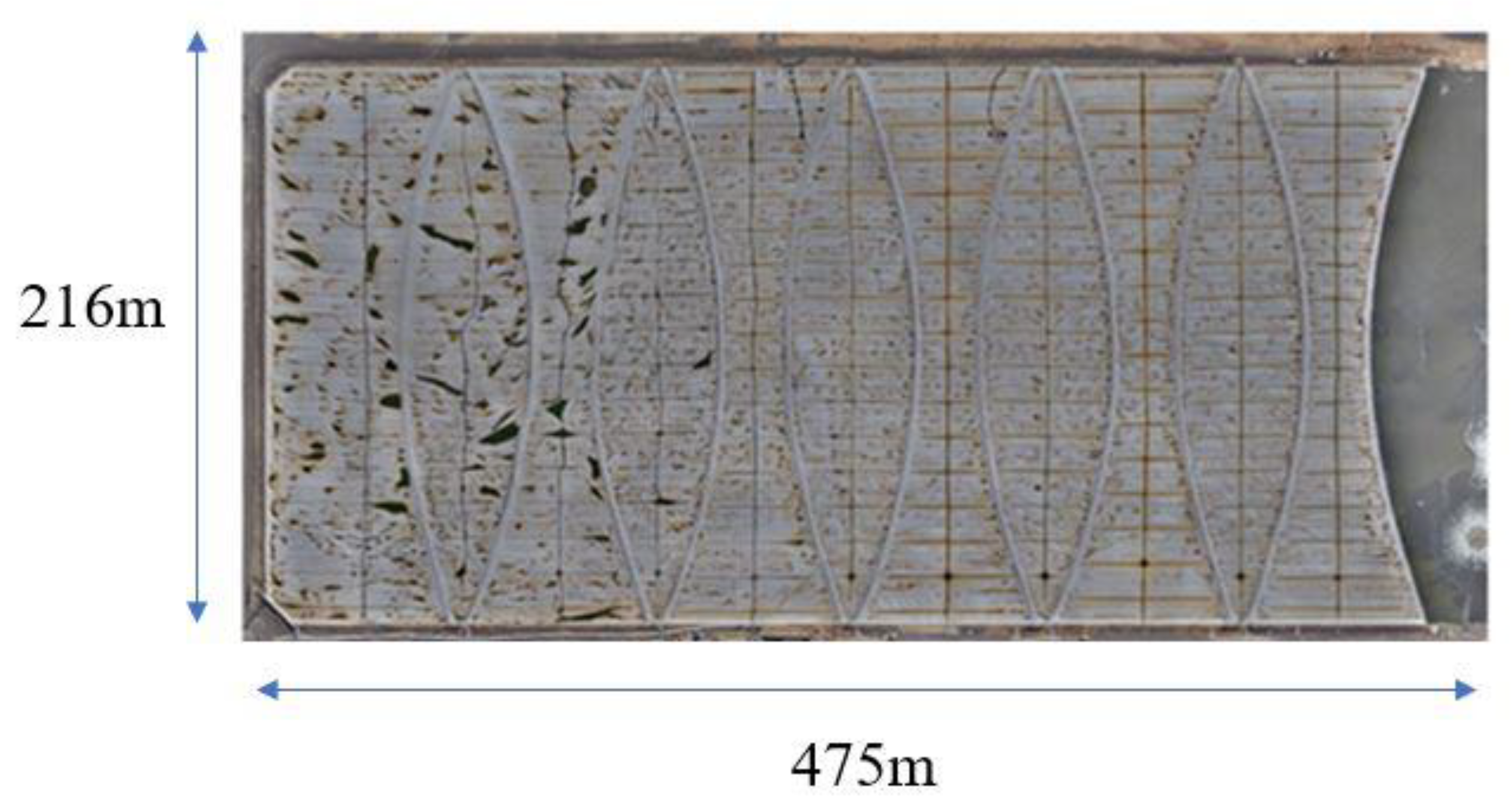
The first treatment lagoons are covered by high-density polyethylene (HDPE) sheets which are seam-welded together [1] to capture all odorous and greenhouse gases (e.g., hydrogen sulfide, methane) produced by the bacteria in the sewage under the covers. These HDPE covers are also known as floating covers since they are fixed to a concrete structure around the perimeter of the lagoons and the surface of the cover rises and falls (i.e., floats) with the changing depth of sewage. A satellite photo of a floating cover at the WTP is shown in Figure 1. Each of the HDPE covers is approximately 475 m long by 216 m wide by 2 mm thick and can collect up to 65,000 cubic meters of biogas per day, which can produce 7 MW of renewable energy [2]. This is more than enough power to sustain the daily operation of WTP and surplus electricity is exported from the site to the grid.
As the raw sewage is untreated before entering the lagoon system, some content such as fats, oils, floating solids and buoyed sludge or other fibrous materials in the raw sewage may separate out of the liquid sewage and float to the surface of the lagoon [3]. These elements can form into a solid mass called “scum”. The scum in the anaerobic lagoon is a mixture of floating solids, undigested sludge and trapped gases formed during anaerobic digestion. This scum can become buoyant and accumulate under the cover and develop into a large solid body, creating an iceberg like effect, which is also called “scumberg” effect because some is above the surface of the water (under the cover) while some stays below the surface. The scum has the potential to move under the surface and even attach itself to the underside of the floating covers. Scum can move and grow over time with varying volume and hardness. The development of scum will exert the following influences on the cover:
- Scumbergs block the pathway of biogas and produce “whaleback” regions on the surface of the cover, affecting the movement and collection of biogases by the covers. Whaleback regions will generate regional strain and stress on the HDPE geomembrane material.
- The existence of scumbergs causes a vertical displacement of the membrane surface. When the wind blows over the cover, the cover will then be exposed to an increased lateral drag force, which can affect the structural integrity of the cover.
- If the scum has developed a hard crust, this may scratch the under-surface of the cover, if the scum moves horizontally and has not yet attached itself to the cover, and potentially result in the development of highly localized non-through cracks which have the potential to become a through-crack.
- Scumbergs can deform the covers in a vertical direction and have an impact on its structural integrity which might then be made even worse when the accumulated scum move under the cover, as any horizontal movement will also exert lateral drag on the covers if the scum has attached itself to the underside of the cover material.
Therefore, the development, accumulation and potential movement of solid scumbergs will adversely affect the structural integrity of the floating covers at the primary treatment lagoon and, thus, there would be benefit in being able to monitor the transition of scum from a semi-solid to a solid state, and the presence and distribution of scumbergs. At present, the physical walk on the cover and visual inspection of the cover are the main methods deployed to determine the distribution and extent of semi-solid to solid scum and scumbergs. The inspection process is labor intensive, time-consuming and involves some inherent risks which we aim to eliminate or reduce. A more quantitative, automated, effective and safe technique is sought to accurately determine the presence of scum and scumbergs under the floating covers without the need for a worker/inspector to physically make contact with the cover.
Due to the size of the lagoon and the hazardous environment, a remote sensing capability is preferred. In this paper, a method of quasi-active thermography is proposed to determine the existence and the extent of the scum under a geomembrane cover with the aid of ambient solar radiation. The newly proposed method is examined under laboratory conditions using an outdoor test facility at Monash University. Whilst the scale of the laboratory test specimen is small in comparison to the actual cover, the study reported in the paper yielded important and useful information for the adaptation of this novel thermographic technique to determine the extent of scum accumulation under the large HDPE floating cover at the WTP. In the experiment reported in this paper, the actual HDPE cover material is used. The solid scum is simulated using solid matter (i.e., a clayey soil) as this was reported to have similar thermal properties to the solid scum at WTP. The HDPE cover was laid over the simulated scum (i.e., a block of clayey soil). The outdoor test facility allowed for investigations into the appropriateness of the different timescales associated with the varying solar radiation for determining the presence and the extent of simulated solid scum under the cover material. It was found that the thermal transients during daybreak and nightfall can be used to determine the existence and accumulation of the clayey soil block under the HDPE geomembrane.
2. Quasi-Active Thermographic Method
2.1. Preliminary Concept of Quasi-Active Thermography
Infrared thermography is a well-developed non-contact inspection technique that has been successfully implemented in the field of structural health monitoring especially for concrete buildings, bridges, rail infrastructure and aircraft structures. These infrared thermal cameras can be located more than 20 m away from the object to be inspected or monitored. Thermography measures the temperature distribution of an object by detecting the infrared energy emitted over an area. It uses differences in temperature to identify the flaws (i.e., cracks, stress concentration area and substance or damage beneath a surface) in the object. In addition, thermal imaging has recently been widely applied in evaluating the structural health condition of composite structures [4,5,6] and polymers [7,8,9,10,11].
Thermography is generally classified into (1) active thermography and (2) passive thermography [12,13,14]. Active thermography [15,16,17,18] requires the monitored object to be subjected to some external source of thermal energy that acts as a stimulus. The input heat energy will penetrate the test specimens and the regions with different properties, such as defects in specimens, will then become obvious in thermal images due to the different responses to the transient heat flow through the object [12]. For example, Genest et al. [15] deployed pulsed thermography (PT) to inspect the deformation growth in bonded graphite repairs of aircraft structures. They used a commercial PT system to trigger the temperature gradients on specimens and the damaged regions showed the same profiles as in ultrasonic inspections. Zeng et al. [18] conducted PT experiments to predict the depth of defects where the defects were in contact with objects in a different phase (water, oil and wax). Breitenstein et al. [19] inspected the defects of silicon solar cells using lock-in thermography. In contrast, passive thermography [20,21] does not require an external source of heat and instead relies solely on the object’s natural variation in heating and/or cooling when exposed to ambient conditions. Kroll et al. [21] monitored the gas leakage of an iron pipe. The leak was detected by the thermal camera when a temperature field disturbance occurred. Steinberger et al. [10] also used passive thermography to monitor the development of fatigue damage during the tension test of carbon fiber reinforced polymer composites. They found that localized heat variation can be detected and used to identify the early stages of damage growth. In addition, thermal imaging is used to inspect large-scale structures such buildings [22] and the oil shale mining [23] by measuring temperatures with thermal imaging. Both active thermography and passive thermography aim to produce the thermal contrast between anomaly parts and surroundings.
The challenges posed by the sheer size of the cover makes conventional thermography impractical, and the flammable biogas generated in the sewage under the covers precludes the use of any powered equipment in the vicinity of the floating cover. In addition, safe work practices dictate any equipment used near the covers is to be intrinsically safe, and no heat or ignition source is to be within a horizontal or vertical distance of 20 m of the anaerobic lagoons. For active thermography, traditional methods of heating such as by halogen lamps, hot air guns or ultrasonics are both unsuitable and impracticable as they cannot heat up such a large region uniformly and simultaneously. Similarly, the use of conventional passive thermography is not applicable since the defects or variation in the covers of themselves do not cause or result in localized heating or cooling of the cover. Moreover, the task of identifying solid matter under the cover is not the same as identifying defects within the cover material—both are useful to know, but they are very different things that require quite different intervention actions at WTP. Therefore, a more practical thermography method is needed that uses a naturally occurring heat stimulus that impinges on the surface of the cover to assess the structural integrity of these large membrane-like floating covers. As a variation to passive thermography, the naturally occurring heat stimulus (i.e., solar radiation) is measured and the associated timescale is acquired and utilized in the analyses of the results. In the proposed experimental inspection method, it was found that the transient geomembrane temperature variations due to daily solar intensity cycles will facilitate the detection of solid matter in contact with the underside of the cover material. In the daytime, solar radiation from the sun’s emissions continuously heat the membrane, and this is similar to the heat up process in classic active thermography. Then in the afternoon, as the solar intensity at the surface of the cover decreases with the setting of the sun, the membrane cools down by convection heat transfer and a transient temperature decay event begins on the membrane. This process lasts for the whole night until the solar intensity increases again from zero at sunrise, and the transient cooling event ends at this point. The proposed method uses naturally occurring heat from the environment, and no heating or cooling system is deployed during the experiment. In addition, the heat power and the way of heating are not controlled, and the heat period is much longer than traditional active thermography. The input heat will not be withdrawn during the monitoring (solar radiation still exists when the radiation power is reduced during the cooling). Given that this thermal imaging method does not monitor the self-heating objects and used external heat as a stimulus, this proposed thermal imaging method is termed quasi-active thermography.
In this paper, long duration thermal imaging experiments were conducted at an outdoor test facility at Monash University. The aim was to determine the measurement parameters to detect the existence and the accumulation of solid matter under the cover material that replicates the scum at WTP. A clayey soil was used in experiments, as this was easier, cleaner and safer to manipulate in an experimental set-up. The main aim of this laboratory-scale tests was to establish the appropriate measurement principles and the associated analyses settings required to quantify the extent of the solid matter covered by the geomembrane. The clayey soils are known to have similar thermal conductivity [24,25], specific heat capacity [26,27] and density [28,29] with the scum, and the scum is difficult to obtain without lifting a section of the cover. The transient events generated by the time varying solar radiation were captured by the pyranometer, which was used to record the solar intensity and to define the start points and the end points of these transients. The HDPE geomembranes that was laid over the clayey soil was exposed to the sun for several days, and the temperature profiles of the geomembrane recorded by the thermal camera were analyzed in conjunction with the solar radiation data.
2.2. Newton’s Law of Cooling for Quasi-Active Thermography
Newton’s law of cooling [30] is a rule to describe the cooling process of objects that are exposed to a cooler ambient temperature. Newton’s law of cooling states that the rate of temperature reduction of an object is proportional to the temperature difference between the surface of the object and the ambient temperature. The relation is demonstrated as:
After integration and defining the initial condition, the solution of this equation becomes:
where is the surface temperature of the object, t is the time, is the ambient temperature, is the initial temperature of the object and k is the cooling constant which governs the rate of the temperature reduction during cooling. In the convection heat transfer process, the cooling constant k [30] reveals how fast the temperature of the object decays to the surrounding temperature, and it can be defined through the equation as shown below:
where is the Nusselt number, is the gas thermal conductivity, and is the characteristic length. When different kinds of material are exposed to the same cooling conditions or environment, the rates of cooling for these materials are different due to the varying film condition coefficients, thus resulting in different values of cooling constants. Moreover, when the material is in contact with other objects, the cooling constants of the material will be affected by transient heat transfer via the material thermal conductivity.
In this paper, Newton’s law of cooling is used to identify where the underside of the HDPE geomembrane material is in contact with the clayey soil as simulated solid scum. This is intended to be analogous to the situation at WTP where the sections of the floating covers in contact with the scum are expected to have a different temperature change rate to the geomembranes in contact with liquid sewage or biogas. Given the temperature gradients between the scum regions and regions not in contact with the scum are constantly responding to the changing solar intensity, it will be difficult to use a single frame of a thermal image to identify the regions of the cover in contact with the scum by just using the temperature contrast. Therefore, the proposed quasi-active thermography uses the different thermal transients acquired to identify the regions of HDPE geomembranes sample that is in contact with clayey soil. The pyranometer provides important information to facilitate the determination and acquisition of appropriate transients over a defined time period during which a sizeable transient can be used to direct the acquisition of useful data to determine the existence and quantify the size of clayey soil under the cover. These thermal transients will be analyzed using the temperature data contained in the acquired thermal image sequences. The transient curves are smoothed and fitted in Newton’s law of cooling and the resultant values of cooling constants k are plotted in a map. Then, parts of the geomembrane in contact with sub-surface objects will appear in strong contrast to the parts without sub-surface objects.
3. Proof of Concept (Quasi-Active Thermography)
3.1. Experiment Setup
A 2 mm thick sheet of HDPE geomembrane (provided by Melbourne Water Corporation) was cut into a size of 1.1 m by 0.8 m and fitted to the frame of a test container as shown in Figure 2a. The membrane specimen is the same material that is used to cover the first part of the anaerobic lagoons at WTP. The emissivity spectrum of the HDPE geomembrane was tested using Fourier-transform infrared (FTIR) spectroscopy in laboratory. Several pieces of HDPE geomembrane samples in WTP were tested. Figure 2b shows the resultant emissivity spectrum of the HDPE geomembrane material. The FTIR result shows that the test sample has a high emissivity (above 95%) within the long-wavelength infrared bandwidth (9–14 µm) confirming that the HDPE geomembrane is suitable for long-wavelength infrared thermography inspection.
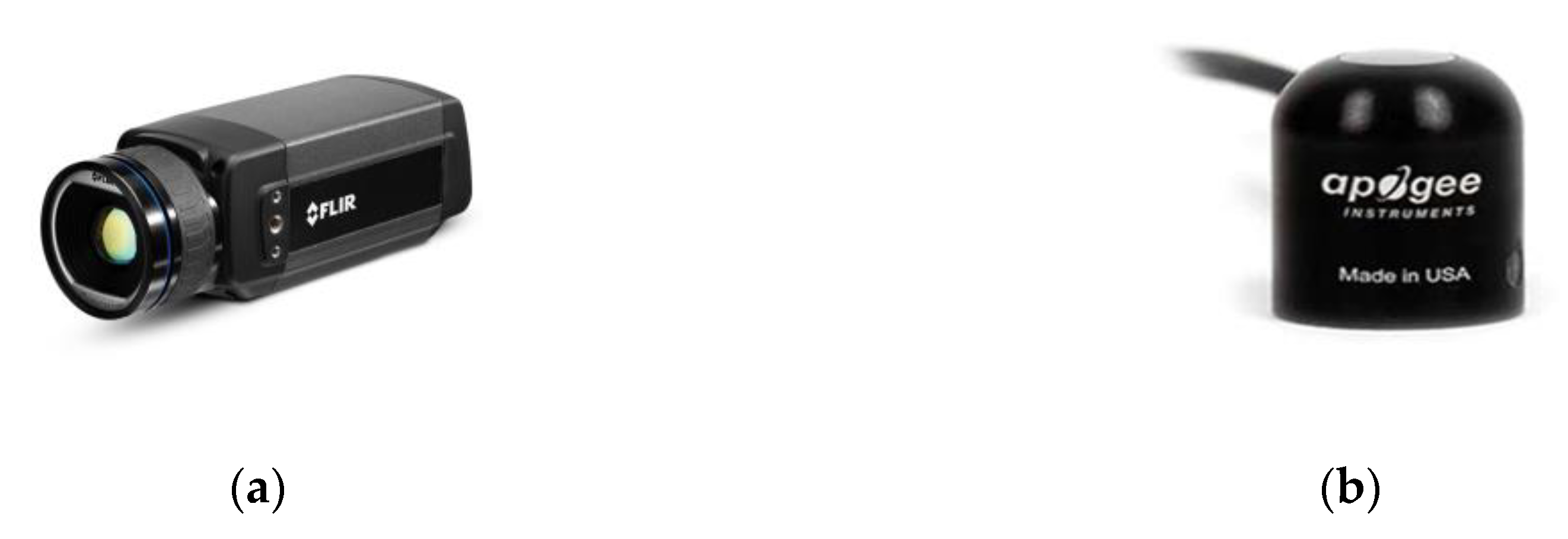
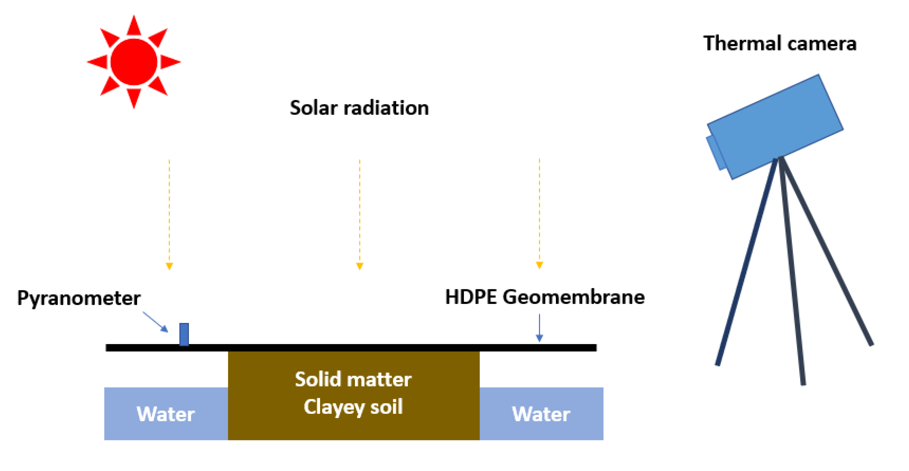
A solid block of clayey soil with an area of 0.15 m by 0.15 m was compacted in 0.1 m deep rectangular aluminum containers (1.1 m by 1.1 m), as shown in Figure 3, and was used to simulate the scum at WTP. The prepared HDPE sheet was then clamped onto the aluminum container (see Figure 2a) with the underside of the center portion of the HDPE geomembrane resting on the top surface of the clayey soil. The entire set up was then moved to an open, outdoor area on a cloudless day. A long-wavelength infrared thermal camera, FLIR A615 (manufactured by FLIR Systems, Inc. Wilsonville, OR, USA) with a resolution of 640 by 480 [31] was set up to record the surface temperature of the cover. The temperature measured by thermal camera was verified by a thermal couple in the laboratory, and the difference is within ± 0.01 °C, which is within the temperature sensitivity of the thermal camera. The solar intensity at the test site was measured using an Apogee SP-110 pyranometer (manufactured by Apogee Instruments, Inc. Logan, UT, USA) [32]. Figure 4a,b show the long-wavelength infrared thermal camera FLIR A615 and the Apogee SP-110 pyranometer, respectively. The schematic diagram of the experimental set up is shown in Figure 5. In this paper, the start and end points of transient events are shown in 24-h format. The experiment was conducted in winter in which the reliability of the quasi-active thermography can be verified with a low level of solar radiation (stimulus). The experiment ran overnight starting from 13:01:13 on the first day until 14:14:33 on the second day. Both thermal camera and pyranometer were collecting the data at a sampling rate of 3 Hz.
3.2. Cooling Constant Estimation Using Newton’s Law of Cooling
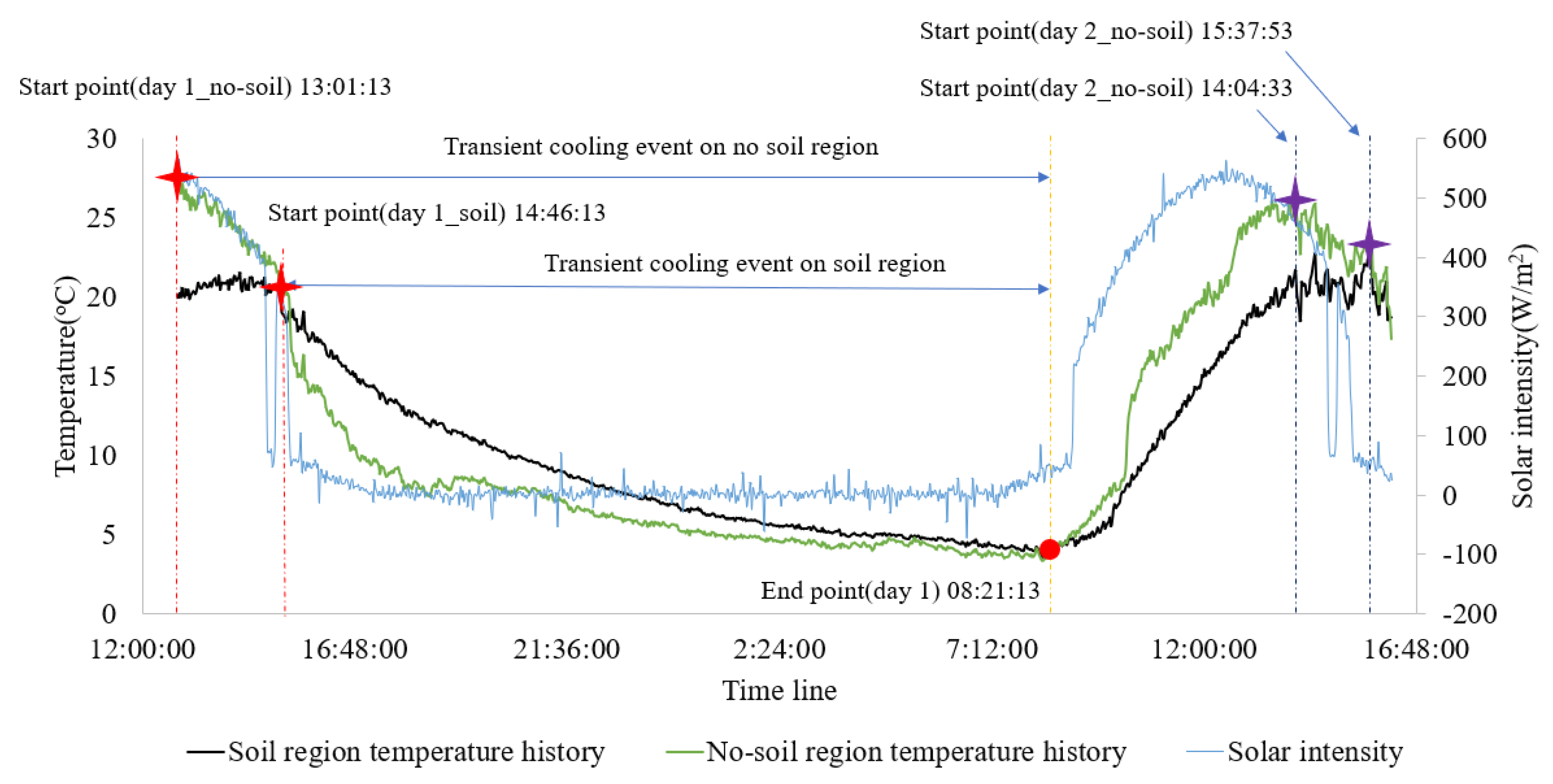
One transient cooling event is expected to commence during the experiment in the afternoon. Since the location of the under-surface soil is known, two points on the HDPE geomembrane were chosen for comparison, one was selected at the point where the geomembrane is in contact with the block of clayey soil, and another point was selected at a point away from where the simulated scum under the geomembrane. The temperature information at both points was extracted from all the obtained thermal images (during the experiment) and plotted in Figure 6. Different points on the same region will have slightly different temperatures, but this will not affect the whole cooling process. The solar intensity data obtained from the pyranometer is also shown in this figure. The reduction in the solar intensity shown in the figure is recorded as the afternoon progresses. As hypothesized, the thermal response at the regions of the HDPE that is in contact with the soil and those that are not are markedly different.
It is noted that on the first day, the temperature of the HDPE region that is not in contact with the clayey soil started to decrease at 13:01:13, see Figure 6. Similar results were also measured on the second day (after 14:04:33). These points mark the starting point of the commencement of the transient cooling event.
For the points on HDPE in contact with the block of soil, due to the thermal conduction between the soil and the geomembrane, the thermal response is markedly different from the point that on the HDPE that is not in contact with the soil. The thermal transient at the point on the HDPE in contact with the soil commenced at 14:46:13. It appeared at 15:37:53 at the second day. The transient events of both points ended at 08:21:13 on the morning of the second day when the solar intensity increased, and the geomembrane became warmer.
It can be seen in Figure 6 that the rates of temperature decay at the two selected points are quite different (black—point on the HDPE that is in contact with the block of soil and green—point on the HDPE that is not in contact with the soil). Figure 6 shows that the temperature at the measured point away from the soil (green line) responded rapidly with the reduction in solar intensity, whereas, the thermal transient differs markedly at the measured point directly above where the compacted block of soil. This phenomenon can be due to two reasons:
- (1)
- (2)
- the HDPE cover can absorb the heat radiated by the block of soil and air, and a portion of the absorbed heat can be re-emitted back to the soil and the air. The cover material acts like a reflective layer which partially reflects the heat back to the soil and air (absorb from soil and air and re-emitted back to soil and air). The thermal wave reflection coefficient [18] of air interface and soil interface is different, leading to efficiency of heat exchange different between the air/geomembrane medium and the soil/geomembrane medium.
These are the principles that are of interest for this experiment, which can be used to identify and evaluate extent of the scum underneath the cover (i.e., at the lagoons at the WTP).
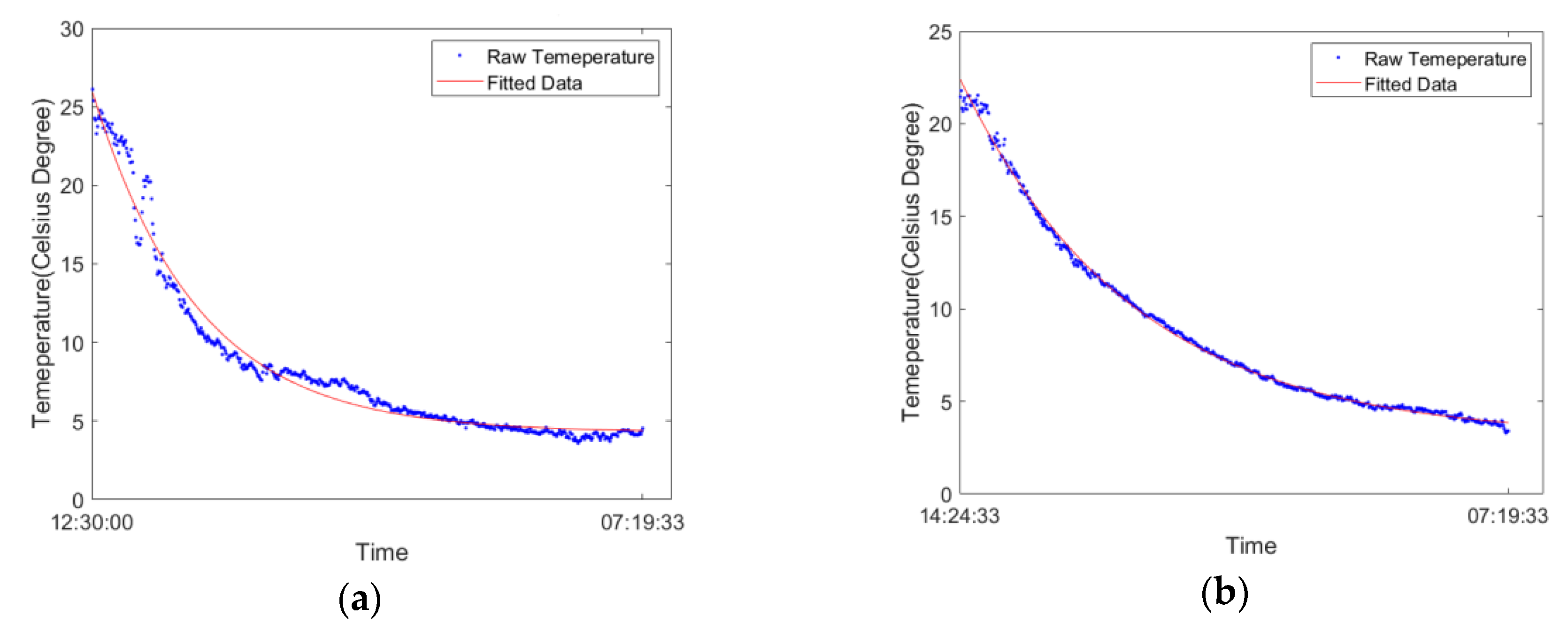
Newton’s law of cooling is used to define the rate of cooling during the thermal transient. The temperature histories during the transient cooling events for both selected points were fitted with Equation (2) using the curving fitting tool in MATLAB. It is noted here in the experiment, the ambient temperature varied with time. While in the curve fitting, the value of was set as the final temperature of the transient event (4.3 °C) and kept as a constant value over the whole event. This is because the cooling constant is proportional to the temperature difference between the ambient conditions and the geomembrane. Varied ambient temperature will make the cooling constant change over time, and the cooling constant will not be consistent in the curve fitting if the ambient temperature changes. Therefore, the curve fitting with Newton’s cooling law in this paper assumed that the geomembrane is cooling in a constant ambient temperature and the resultant efficient cooling constant k can be consistent over the whole event. Given that the temperature of geomembrane changes quite slowly at the end of the event, it was assumed that the geomembrane achieves ambient temperature at this point, and the ambient temperature was set as the value at this point.
Figure 7a,b show the fitted plots for the point away from the block of soil and at the location of the soil, respectively. Table 1 shows the properties of curve fit (R-squared and root mean square error) and estimated cooling constant, k. The result shows that the cooling constant of the no-soil region kno-soil is 0.00925 and the cooling constant of the soil region ksoil is 0.00484. The lower value of the cooling constant of the cover in the region over the soil suggests that the temperature of the geomembrane at this region will decrease slower than that at region not in contact with the soil. This is due to the conductive heat exchange between the HDPE sheet and the soil. The goodness of curve fitting, in the region over the soil gave an R-squared value of 0.9748, which means 97.48% of the temperature data comply with the model of Newton’s cooling law. Furthermore, the RMSE for the region not in contact with the soil region is 0.8675. The R-squared and the RMSE for the soil region also presented a reasonable goodness of curve fitting. Both indexes indicate that the cooling of the HDPE cover in the experiment agrees with Newton’s law of cooling.
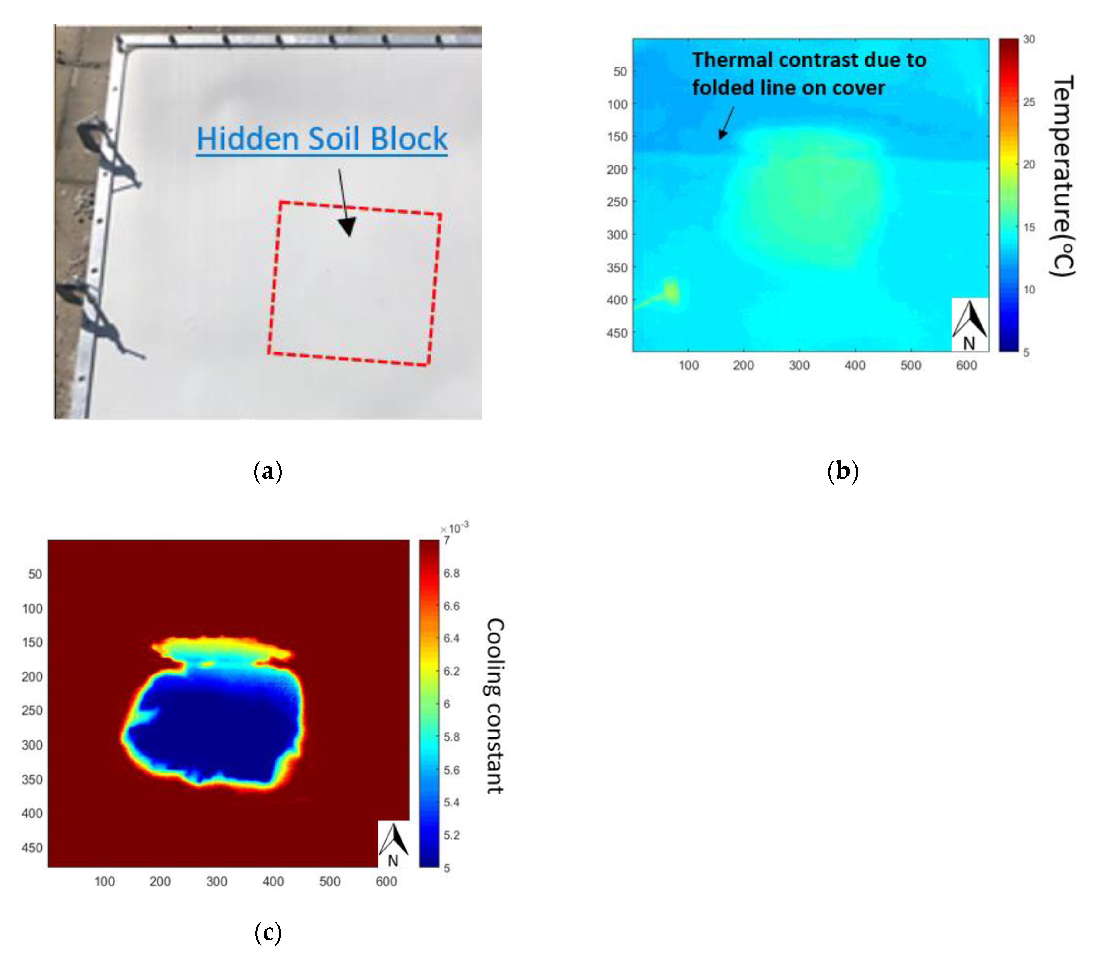
To demonstrate the advantage of this proposed technique, the cooling constant over the entire HDPE sheet is calculated using one transient cooling event. For comparison purposes, the optical image taken of the HDPE material with soil underneath is plotted together with the thermal image at one instant and the resultant cooling constant mapping in Figure 8a–c, respectively. Figure 8a was taken using an optical camera and shows the location of the hidden soil (underneath the cover). Figure 8b shows the raw thermal image taken at an instant (single frame) by the thermal camera during the transient event, a thermal contrast can be seen on the thermal image, however, the difference in temperature between the soil region and no-soil region is small (approximately 4 °C at this instant). As shown in Figure 6, the temperature contrast between the regions with and without the soil changes with the time in a day. The thermal contrast also depends heavily on which frame was chosen for analysis. Moreover, the condition of the cover (i.e., dirt, fold line and view angle) can also affect the accuracy of the temperature measurement.
Figure 8c shows a map (640 × 480 resolution) of cooling constants calculated using Newton’s law of cooling. The cooling constant at the region over the soil was determined to be within 0.005 and 0.007 (with a higher value around the edges of the soil). For better identification of the soil, a color threshold was set to show only the range between 0.005 and 0.007 and the rest was to be red for Figure 8c. The reason to set up this filter is to show the profile of under-cover soil and to eliminate the influence of noisy data. The profile of the soil under the cover can then easily be identified and outline as shown in Figure 8c, and the cooling constant gradient region of the soil is a result of the rough surface of soil and the uneven contact between itself and the cover. The results show a good agreement between the geometry of the actual block of soil with that estimated from the thermal images. This experiment shows that the night period provides enough time for the quasi-active thermography to determine the presence of the soil under the membrane and to facilitate the estimation of the extent of the soil under the membrane. Thus, the proposed quasi-active thermography method is shown to be able to identify the presence and extent of the under-surface soil.
3.3. Experiments to Verify the Consistency of the Quasi-Active Thermography Measurements
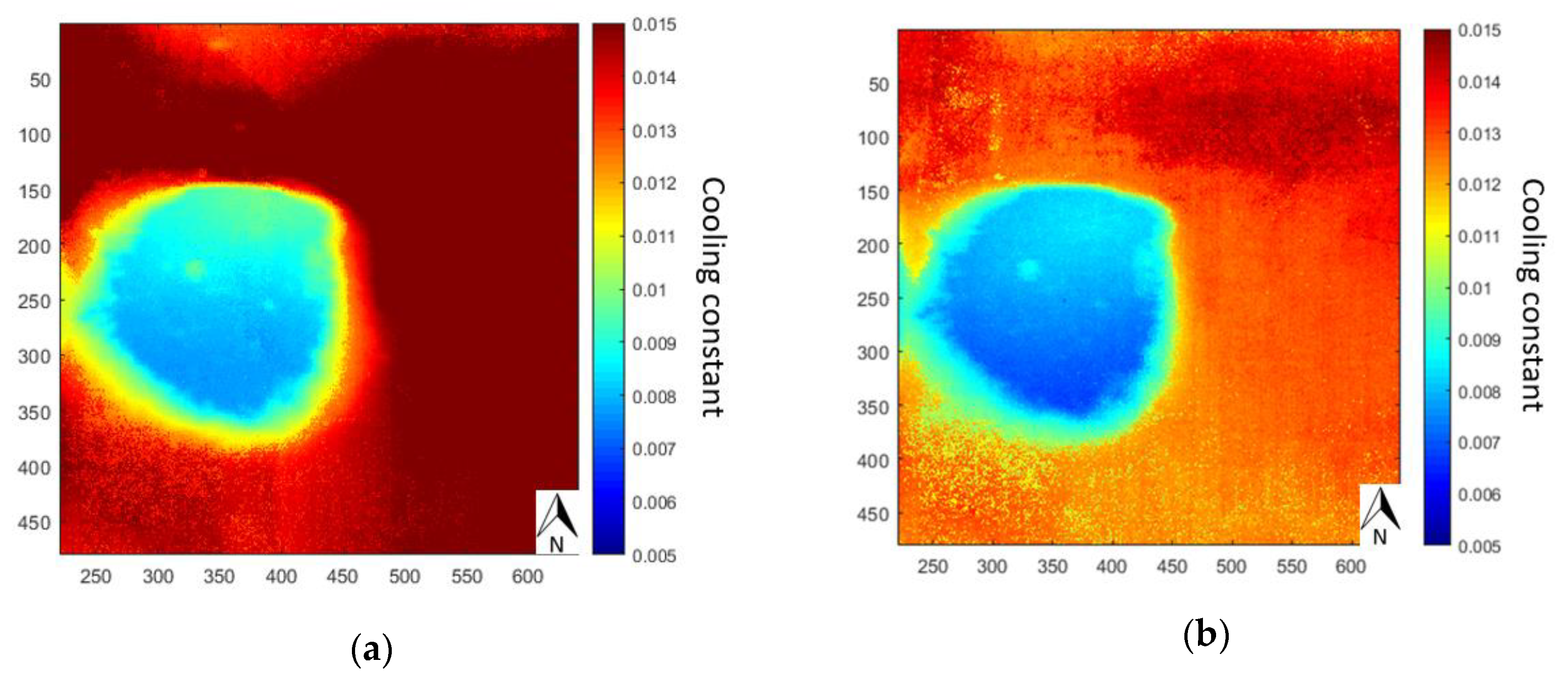
In traditional active thermography inspections, the length of heat up and cool down periods can be controlled, and the input power of heat can also be adjusted. However, in long timescale quasi-active thermography, the length of transient events is determined by the solar intensity. In addition, each transient event is non-repeatable since the daily time from the sunset to the sunrise is different and temperature profiles will also vary from day to day and from season to season. This can lead to a difference in the cooling period of the cover during each transient cycle. The results presented in this section is used to verify the measurement consistency of quasi-active thermography test. A continuous two-day experiment was conducted, and the maps of cooling constants in two transient cooling events were compared to test the consistency of the results. An irregular shape of soil was placed under the HDPE sheet. The same experimental set up (see Figure 5 and Section 3.1) was used and the temperature profile of the top surface of the cover and the solar intensity history were monitored using FLIR A615 thermal camera and pyranometer, respectively. Figure 9 shows the solar intensity profile over two days with temperature history at two selected points on the cover (red line: Point at the soil region and green line: Point away from soil region). Two transient cooling events are also labelled in Figure 9 and the important information of each event are listed in Table 2. Again, Equation (2) obtained from Newton’s law of cooling is used to fit into the transient cooling events for both events at both points and the results are plotted in Figure 10a–d. The estimated cooling constants with R-squared and RMSE of these four curves are reported in Table 3.
It can be observed from Table 4 that the cooling constants on each region on the second day were higher than that in the first day. This is due to the fact that the length of transient event in day two was shorter than in day one, and the initial temperatures of the geomembrane in day two is was higher than in day one. This indicates a faster cooling process in day two, resulting in a higher value of cooling constant for the geomembrane. In addition, the cooling constant for the region of the material over the soil is smaller than that for a no-soil region, and this agrees with the result in Section 3.2. These measurements differences could be due to (1) difference in environment condition (solar intensity, wind speed and ambient air temperature) in each day which affected the heat transfer coefficients, (2) difference in initial temperatures of the cover in each transient cooling event and (3) different condition of contact between the soil and the HDPE material. However, the contrasts of cooling constants between the soil region and the no-soil region are still significant enough to identify the extent of the under-cover soil. Therefore, it can be concluded that the cooling constant in each transient event is different due to the non-repeatable surrounding conditions. Hence, the values of the cooling constant should be normalized in each experiment.
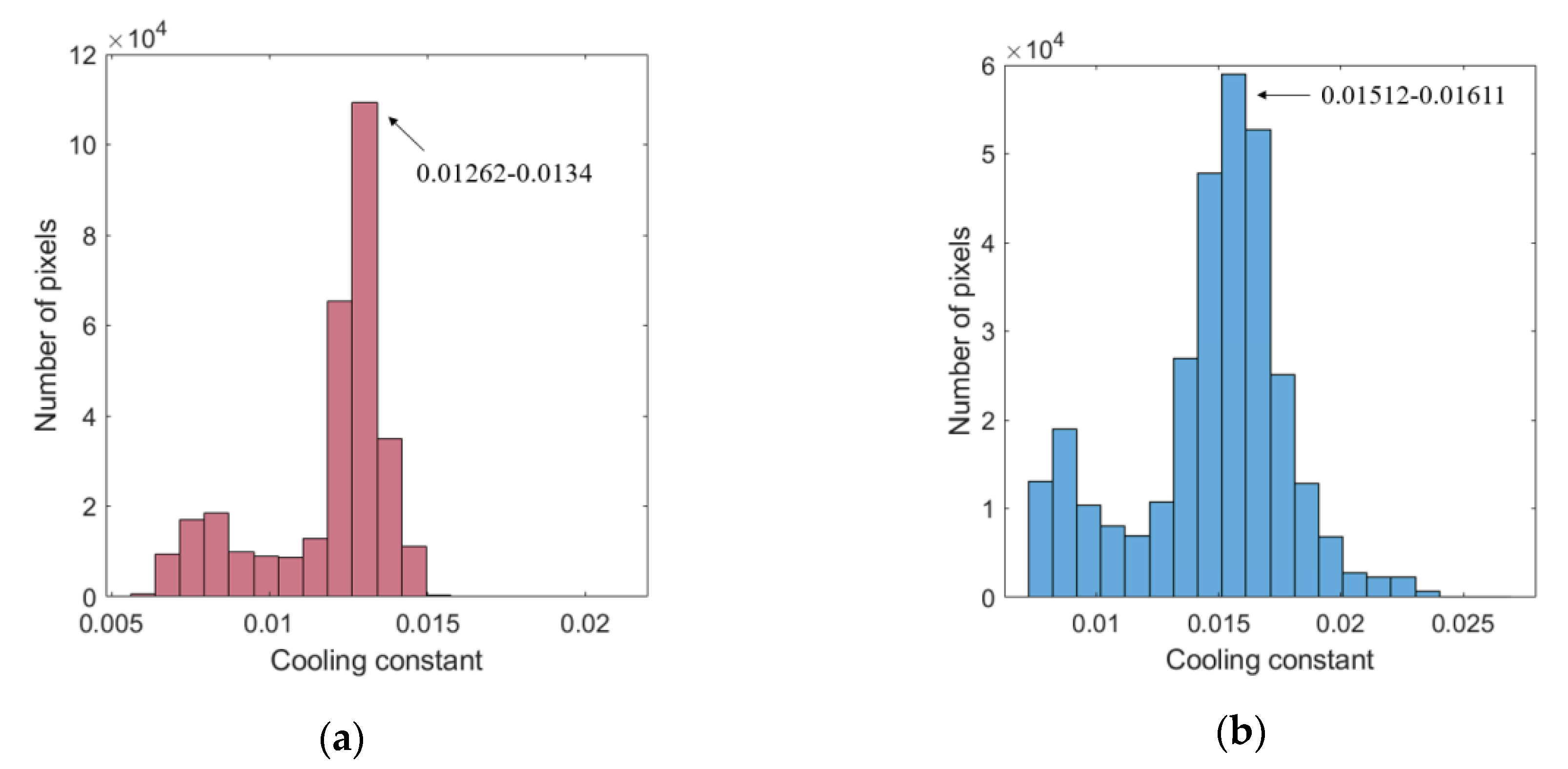
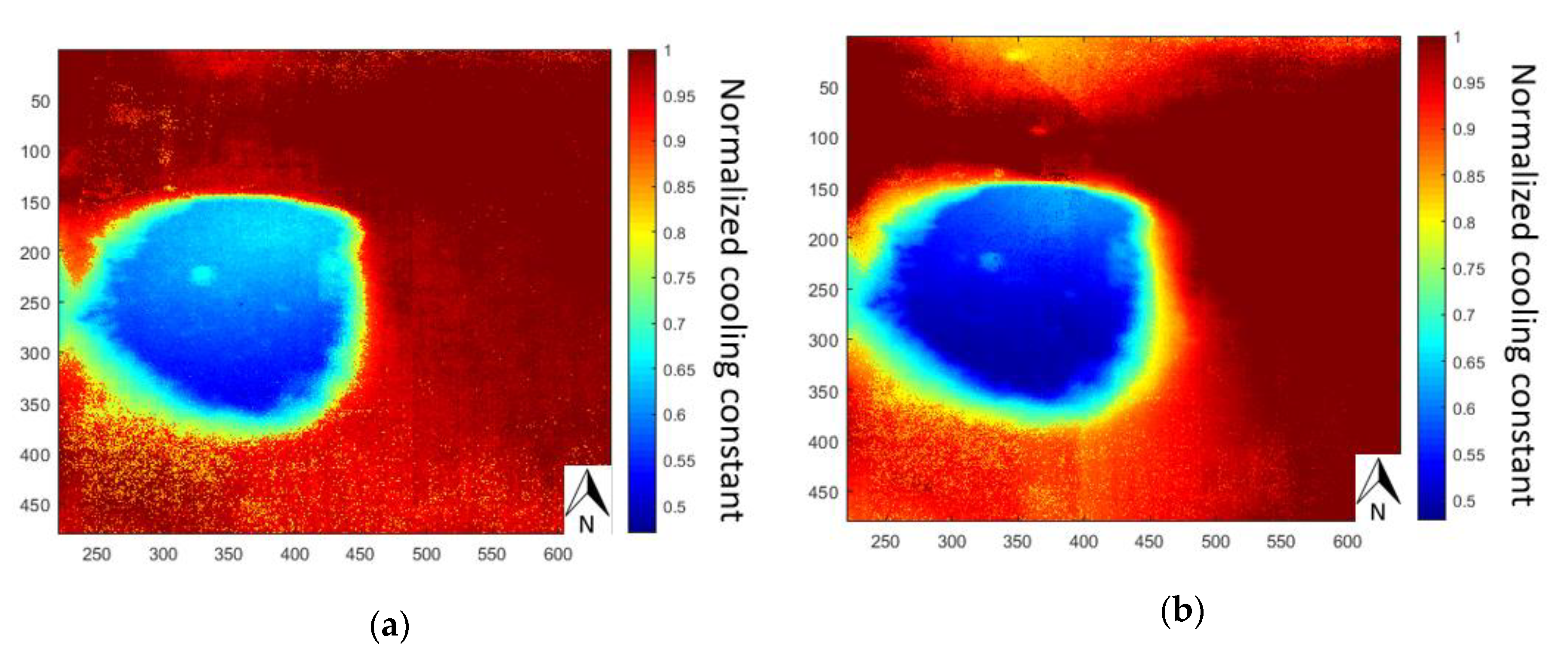
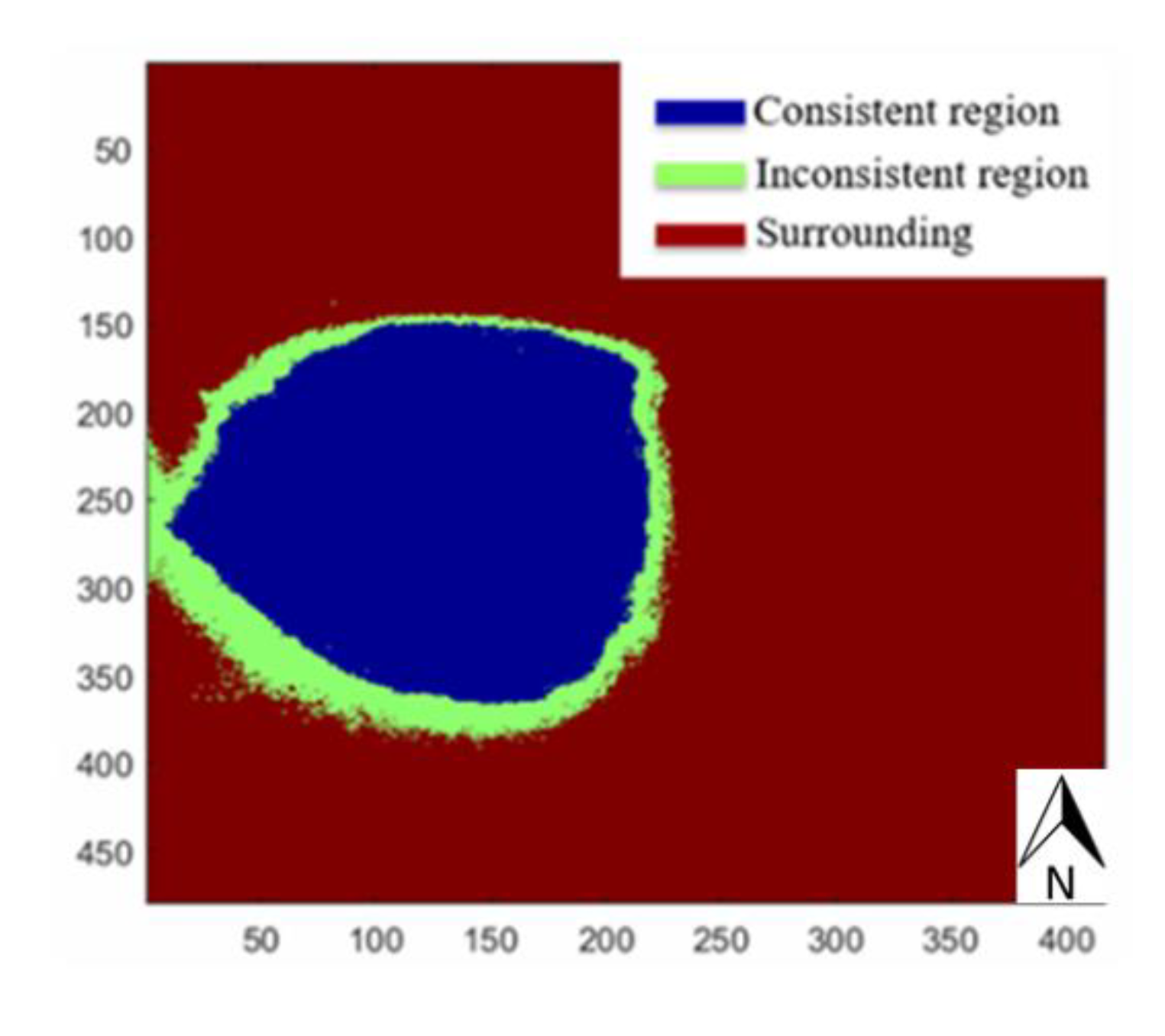
The maps of cooling constants of the membrane over two days were plotted and are shown in Figure 11. The resolution of the image in this experiment is 480 by 420 pixels (i.e., 201,600 pixels). To validate the measurement consistency, a normalization study was conducted to make the threshold of defining the with-soil region the same in two days experiment. The histograms of values of cooling constant are shown in Figure 12 and it can be observed that the values approximate the normal distribution. The cooling constant plot shown in Figure 12 is scaled with respect to the peak value shown in Figure 12. The cooling constants maps in Figure 11 were divided by the background spans (0.01262 in day one, 0.01512 in day two) and the normalized maps are plotted in Figure 13. The upper limit of the threshold is set as 1 given that the cooling constant at the region over the soil region is always lower than the background. It can be observed that the normalized cooling constant of the soil region is roughly lower than 0.65. A statistical study of the threshold to determine the region of soil in the cooling constant map was conducted with a 0.05 step change in the up limits of normalized cooling constant. Table 5 shows the comparison of the area of soil region in two days experiment. 2.94% mean difference indicates that the quasi-active thermography in two days experiment has a good measurement consistency. This indicates that although cooling constant values change in different transient events, the ksoil and kno-soil will change proportionally, and the results are consistent after normalization. For comparison, the mean soil region areas from the statistical analysis were extracted in MATLAB code and the contrast in Figure 14 shows the difference of measurement. Nevertheless, in each measurement, the proportional contrast in cooling constant between the cover with and no-soil beneath the cover material can still be differentiated easily and can be used to define and outline the profile of the soil in contact with the cover. This experiment again provides evidence of the consistency of quasi-active thermography measurements with different ambient temperature profiles and lengths of transient events.
4. Quasi-Active Thermography Monitoring of Accumulation of Soil Buildup under the HDPE Membrane
In Section 3, the quasi-active thermography monitoring has successfully demonstrated its reliability, repeatability and capability to identify and locate the soil underneath the cover material. In this section, quasi-active thermography monitoring is further examined to monitor the development (growth) of soil experimentally to simulate the expansion of the area of scum under the HDPE covers on the anaerobic lagoons. To accomplish the aim, the same experimental setup, as described in Section 3.1, is used. A multiple-day quasi-active thermography experiment was conducted with more compacted soil added to the aluminum container each day (i.e., to simulate the growth in the extent of the scum at WTP).
On the first day of the experiment, a block of soil (of approximately 10 kg) was compacted in a corner in the aluminum container. The prepared HDPE sheet was then covered over the aluminum container. Both the infrared thermal camera and pyranometer were set up to collect data at 3 Hz starting at 12:00:00. The second day at noon, the HDPE cover was first removed, and an additional 20 kg of soil was then compacted around the existing soil to simulate the buildup of scum. The recordings were resumed after replacing the HDPE cover. The same simulated growth of the soil was repeated on the third day of the experiment by adding approximately 40 kg of garden soil. The overall recording of data ended at 9:30 AM on the fourth day.
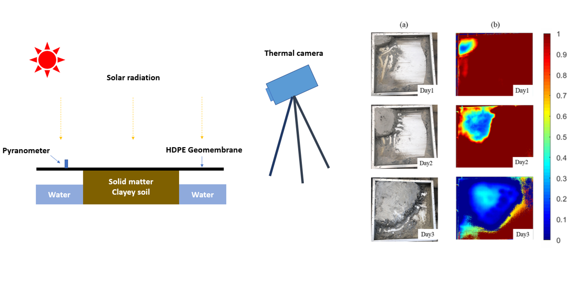
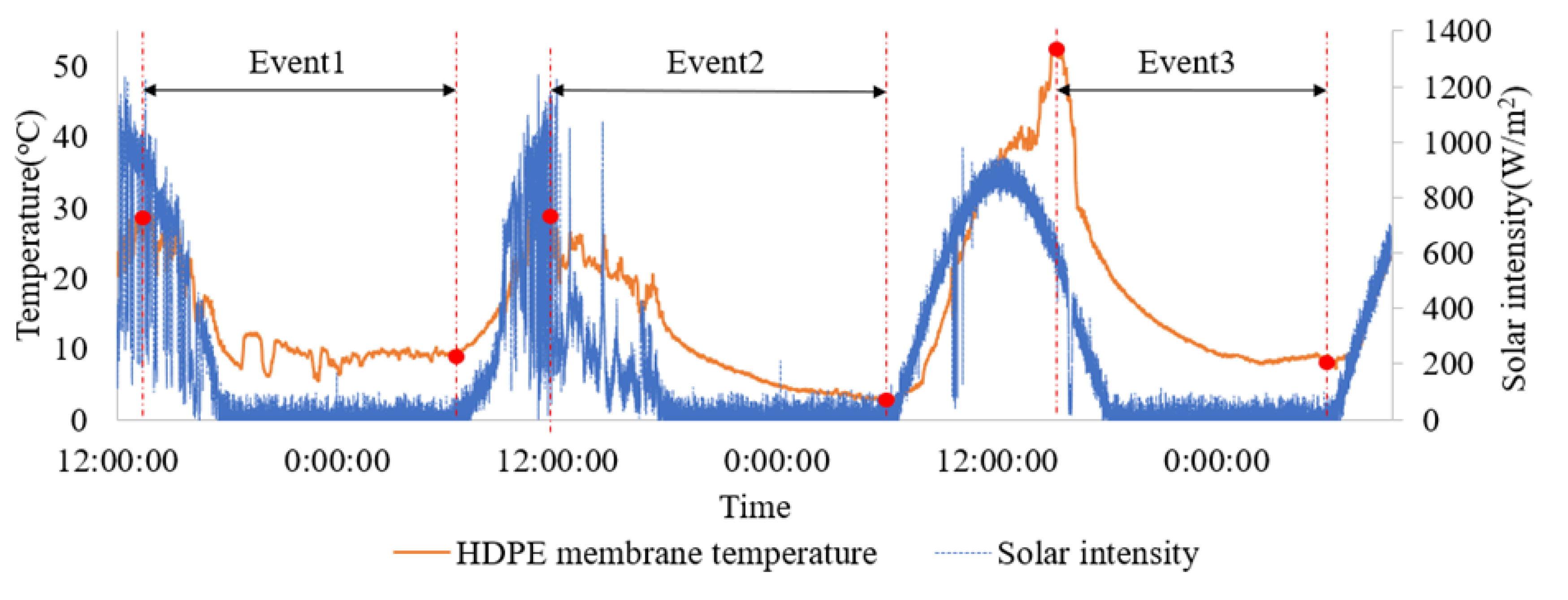
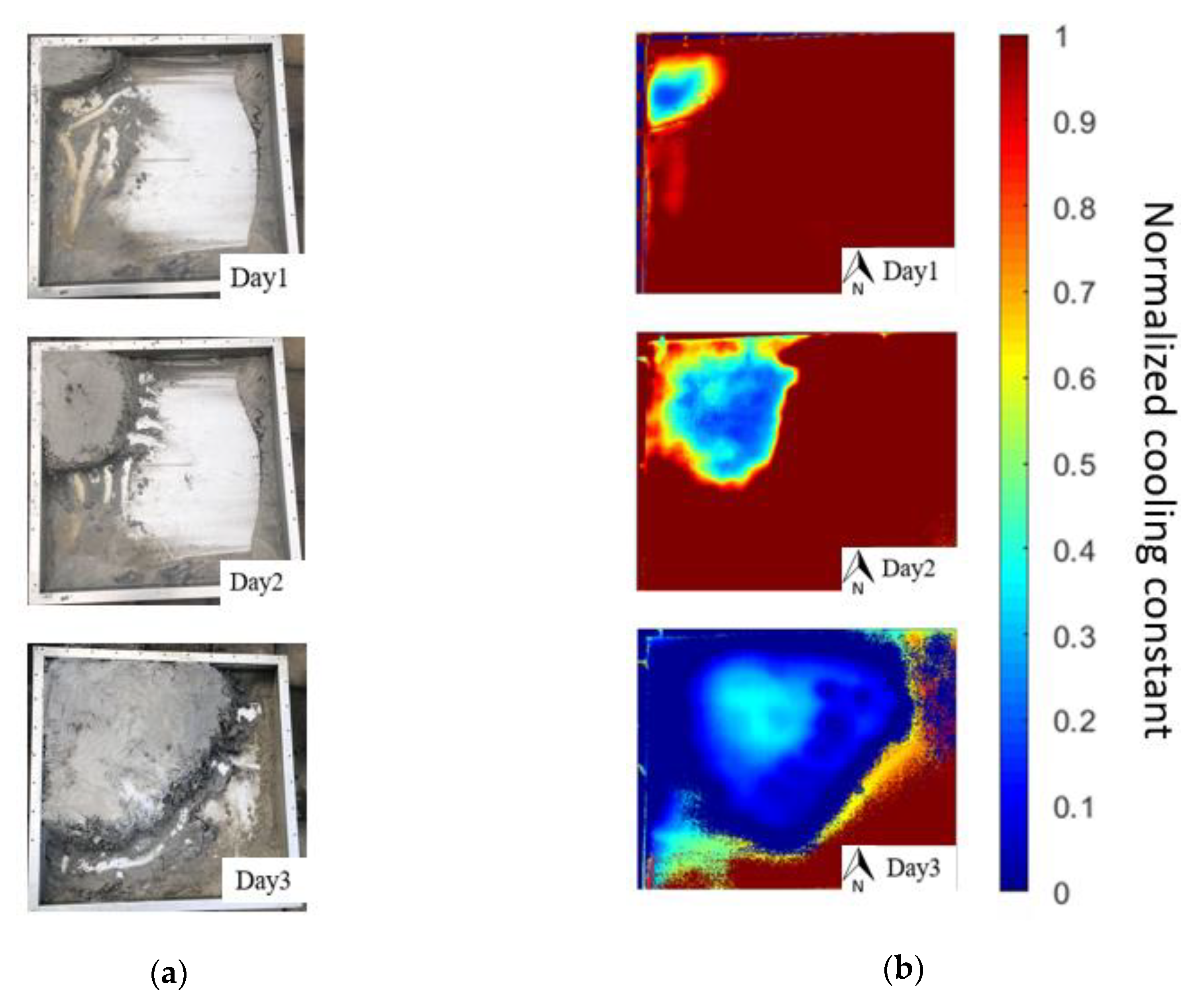
The temperature history at a selected point (away from the soil region) on the membrane and the local solar intensity history are plotted in Figure 15. The solar intensity history shows more fluctuation in signal in the first two days during the daytime, this is indicating that these days were relatively cloudy. Whilst the solar intensity on the third day changed smoothly, showing that this day was a relatively clear day with little cloud cover. Throughout the entire experiment, three transient cooling events were identified, and the period of each event is defined in Figure 15 and listed in Table 6. Each of the transient cooling events were again analyzed using Newton’s law of cooling. Since the scale of cooling constant is different in each day, the scales of cooling constant were normalized again from 0 to 1. The optical photos of the condition underneath the cover and their corresponding zoomed normalized maps of cooling constants for each day are shown in Figure 16a,b, respectively.
Figure 16b shows that the soil underneath the membrane can be identified and outlined using the cooling constant mapping obtained from the cover. In addition, the areas of the soil underneath the membrane were noted to have grown larger every day which agrees with the its geometrical profile as shown in Figure 16a. Although the HDPE cover was disturbed every day, the outcomes are still very promising for monitoring the development of the scum beneath the covers at WTP.
The newly proposed technique—quasi-active thermography has thus far shown its capability to identify, outline and monitor the growth of solid matter (i.e., a clayey soil) underneath the HDPE geomembrane material. The technique can potentially be extended to a field trial in the near future, to determine the location and extent of semisolid and solid scum under the large floating covers at the WTP. The quasi-active thermography has been verified, examined and showed its potential application in the paper. Further research can also be done by using the same proposed technique to evaluate the structural integrity of the large floating cover.
5. Conclusions
In this study, quasi-active thermography has been introduced, validated and examined experimentally to detect the presence and the expansion of soil under HDPE geomembrane material. The proposed technique uses naturally occurring transient cooling events resulting from daily solar intensity cycles. These cooling cycles are defined by the pyranometer data acquired. The temperature profiles of the transient cooling event can then be analyzed using Newton’s law of cooling. By estimating the cooling constant at every monitored point, a map of cooling constant distributions based on the rate of cooling can be constructed, and the results have successfully demonstrated the advantage of the cooling constant mapping to identify, outline and monitor the extent of under-surface soils. The following are the observations and summary of the outcomes of this newly proposed technique:
- Solar radiation can be employed as the external heat source in thermography since the solar energy is economical and is uniformly applied over a large surface area. By monitoring the solar intensity via pyranometer, full transient cooling events can be determined starting when the solar intensity begins to decrease and ending at the time when solar intensity increases from zero.
- Single frame of thermal imaging can be used to show the thermal contrast at some particular time, however, it is influenced by other factors which include condition of the monitoring surface, angle of view of the camera and presence of wrinkles. By monitoring the entire cooling history of the cover, a map of cooling constant can be constructed which enhances the identification and definition of the objects attached underneath the HDPE covers. The results show that the map of cooling constants is more reliable than only relying on the thermal contrast based on a single frame of the thermal image.
- The cooling constants in different transient cooling events can be varied day to day, due to the weather conditions, ambient temperature, wind strength, cloud conditions and solar intensity. This is causing the temperature changes and lengths of cooling events of each day to be different. A multiple-day experiment was conducted to compare results in different days, and the result showed that the cooling constant (rate of cooling) is noted to be significantly different between the no-soil region and soil region in the map of cooling constants. The measurement consistency was verified by normalizing the cooling constant in two transient events. The results have evidence that the proposed monitoring technique is repeatable and reliable.
- The proposed quasi-active thermography inspection is also further examined to monitor the growth of the under-surface objects. The outcomes have demonstrated its potential for field trial to inspect the accumulation of scum at the anaerobic lagoon at the WTP and evaluate the extent and location of scum.
Author Contributions
Conceptualization, Y.M., L.W., B.S.V., and W.K.C.; methodology, Y.M., L.W., B.S.V., and W.K.C.; validation, Y.M.; resources, T.K., J.K. and W.K.C.; formal analysis, Y.M.; writing-original draft, Y.M., L.W., B.S.V. and W.K.C.; writing-review and editing, Y.M., L.W., B.S.V., T.K. and W.K.C.; project administration, T.K. and W.K.C.; funding acquisition, T.K., J.K. and W.K.C. All authors have read and agreed to publish version of the manuscript.
Funding
This research was funded by Australian Research Council Linkage Grant (ARC) LP170100108.
Acknowledgments
The Fourier-Transform Infrared (FTIR) spectroscopy conducted by Defence Science and Technology Group is gratefully acknowledged.
Conflicts of Interest
The authors declare no conflict of interests.
References
- Scheirs, J. A Guide to Polymeric Geomembranes: A Practical Approach; John Wiley & Sons: Hoboken, NJ, USA, 2009. [Google Scholar]
- Ong, W.H.; Chiu, W.K.; Kuen, T.; Kodikara, J. Determination of the State of Strain of Large Floating Covers Using Unmanned Aerial Vehicle (UAV) Aided Photogrammetry. Sensors 2017, 17, 1731. [Google Scholar] [CrossRef] [PubMed] [Green Version]
- Aldave, I.J.; Bosom, P.V.; González, L.V.; De Santiago, I.L.; Vollheim, B.; Krausz, L.; Georges, M.P. Review of thermal imaging systems in composite defect detection. Infrared Phys. Technol. 2013, 61, 167–175. [Google Scholar] [CrossRef]
- Wong, L.; Vien, B.S.; Ma, Y.; Kuen, T.; Courtney, F.; Kodikara, J.; Chiu, W.K. Remote Monitoring of Floating Covers Using UAV Photogrammetry. Remote Sens. 2020, 12, 1118. [Google Scholar] [CrossRef] [Green Version]
- Swiderski, W.; Vavilov, V.P. IR thermographic detection of defects in multi-layered composite materials used in military applications. In Proceedings of the 2007 Joint 32nd International Conference on Infrared and Millimeter Waves and the 15th International Conference on Terahertz Electronics, Cardiff, UK, 2–9 September 2007; pp. 553–556. [Google Scholar]
- Avdelidis, N.; Hawtin, B.; Almond, D. Transient thermography in the assessment of defects of aircraft composites. Ndt E Int. 2003, 36, 433–439. [Google Scholar] [CrossRef]
- Omar, M.A.; Hassan, M.; Donohue, K.; Saito, K.; Alloo, R. Infrared thermography for inspecting the adhesion integrity of plastic welded joints. Ndt E Int. 2006, 39, 1–7. [Google Scholar] [CrossRef]
- Flores-Bolarin, J.; Royo-Pastor, R. Infrared thermography: A good tool for nondestructive testing of plastic materials. In Proceedings of the 5th European Thermal-Sciences Conference, Eindhoven, The Netherlands, 18–22 May 2008. [Google Scholar]
- Dassisti, M.; Intini, F.; Chimienti, M.; Starace, G. Thermography-enhanced LCA (Life Cycle Assessment) for manufacturing sustainability assessment. The case study of an HDPE (High Density Polyethylene) net company in Italy. Energy 2016, 108, 7–18. [Google Scholar] [CrossRef]
- Steinberger, R.; Leitão, T.V.; Ladstätter, E.; Pinter, G.; Billinger, W.; Lang, R. Infrared thermographic techniques for non-destructive damage characterization of carbon fibre reinforced polymers during tensile fatigue testing. Int. J. Fatigue 2006, 28, 1340–1347. [Google Scholar] [CrossRef]
- Kafieh, R.; Lotfi, T.; Amirfattahi, R. Automatic detection of defects on polyethylene pipe welding using thermal infrared imaging. Infrared Phys. Technol. 2011, 54, 317–325. [Google Scholar] [CrossRef]
- Yang, R.; He, Y. Optically and non-optically excited thermography for composites: A review. Infrared Phys. Technol. 2016, 75, 26–50. [Google Scholar] [CrossRef]
- Bagavathiappan, S.; Lahiri, B.; Saravanan, T.; Philip, J.; Jayakumar, T. Infrared thermography for condition monitoring–A review. Infrared Phys. Technol. 2013, 60, 35–55. [Google Scholar] [CrossRef]
- Kylili, A.; Fokaides, P.A.; Christou, P.; Kalogirou, S.A. Infrared thermography (IRT) applications for building diagnostics: A review. Appl. Energy 2014, 134, 531–549. [Google Scholar] [CrossRef]
- Genest, M.; Martinez, M.; Mrad, N.; Renaud, G.; Fahr, A. Pulsed thermography for non-destructive evaluation and damage growth monitoring of bonded repairs. Compos. Struct. 2009, 88, 112–120. [Google Scholar] [CrossRef]
- Schroeder, J.; Ahmed, T.; Chaudhry, B.; Shepard, S. Non-destructive testing of structural composites and adhesively bonded composite joints: Pulsed thermography. Compos. Part A Appl. Sci. Manuf. 2002, 33, 1511–1517. [Google Scholar] [CrossRef]
- Rajic, N.; Rowlands, D.; Tsoi, K. An Australian perspective on the application of infrared thermography to the inspection of military aircraft. In Proceedings of the 2nd International Symposium on NDT in Aerospace, Hamburg, Germany, 22–24 November 2010. [Google Scholar]
- Zeng, Z.; Li, C.; Tao, N.; Feng, L.; Zhang, C. Depth prediction of non-air interface defect using pulsed thermography. Ndt E Int. 2012, 48, 39–45. [Google Scholar] [CrossRef]
- Breitenstein, O.; Rakotoniaina, J.P.; Al Rifai, M.H. Quantitative evaluation of shunts in solar cells by lock-in thermography. Prog. Photovolt. Res. Appl. 2003, 11, 515–526. [Google Scholar] [CrossRef]
- Taole, R.; Falcon, R.; Bada, S. The impact of coal quality on the efficiency of a spreader stoker boiler. J. South. Afr. Inst. Min. Metall. 2015, 115, 1159–1165. [Google Scholar] [CrossRef]
- Kroll, A.; Baetz, W.; Peretzki, D. On autonomous detection of pressured air and gas leaks using passive IR-thermography for mobile robot application. In Proceedings of the 2009 IEEE International Conference on Robotics and Automation, Kobe, Japan, 12–17 May 2009. [Google Scholar]
- Brooke, C. Thermal imaging for the archaeological investigation of historic buildings. Remote Sens. 2018, 10, 1401. [Google Scholar] [CrossRef] [Green Version]
- Xiao, C.; Fu, B.; Shui, H.; Guo, Z.; Zhu, J. Detecting the Sources of Methane Emission from Oil Shale Mining and Processing Using Airborne Hyperspectral Data. Remote Sens. 2020, 12, 537. [Google Scholar] [CrossRef] [Green Version]
- Song, H.; Park, K.J.; Han, S.K.; Jung, H.S. Thermal conductivity characteristics of dewatered sewage sludge by thermal hydrolysis reaction. J. Air Waste Manag. Assoc. 2014, 64, 1384–1389. [Google Scholar] [CrossRef] [Green Version]
- Wang, K.-S.; Tseng, C.-J.; Chiou, I.-J.; Shih, M.-H. The thermal conductivity mechanism of sewage sludge ash lightweight materials. Cem. Concr. Res. 2005, 35, 803–809. [Google Scholar] [CrossRef]
- Ding, H.-S.; Jiang, H. Self-heating co-pyrolysis of excessive activated sludge with waste biomass: Energy balance and sludge reduction. Bioresour. Technol. 2013, 133, 16–22. [Google Scholar] [CrossRef] [PubMed]
- Wang, Y.; Lu, Y.; Horton, R.; Ren, T. Specific heat capacity of soil solids: Influences of clay content, organic matter, and tightly bound water. Soil Sci. Soc. Am. J. 2019, 83, 1062–1066. [Google Scholar] [CrossRef]
- Zeri, M.; Álvala, R.C.S.; Carneiro, R.; Cunha-Zeri, G.; Costa, J.M.; Spatafora, L.R.; Urbano, D.; Vall·llossera, M.; Marengo, J.A. Tools for communicating agricultural drought over the Brazilian Semiarid using the soil moisture index. Water 2018, 10, 1421. [Google Scholar] [CrossRef] [Green Version]
- Balasubramanian, R.; Sircar, A.; Sivakumar, P.; Ashokkumar, V. Conversion of bio-solids (scum) from tannery effluent treatment plant into biodiesel. Energy Sources Part A Recovery Util. Environ. Eff. 2018, 40, 959–967. [Google Scholar]
- Bergman, T.L.; Incropera, F.P.; DeWitt, D.P.; Lavine, A.S. Fundamentals of Heat and Mass Transfer; Bergman, T.L., Lavine, A.S., Eds.; John Wiley & Sons, Inc.: Hoboken, NJ, USA, 2017. [Google Scholar]
- FLIR. User’s Manual FLIR A6xx Series; FLIR systems: Wilsonville, OR, USA, 2016. [Google Scholar]
- Apogee. Apogee Instruments Owner’s Manual Pyranometer Models SP-110 and SP-230; Apogee: Logan, UT, USA, 2020. [Google Scholar]
- Guo, X.; Zhang, F.; Liu, Y. Study on pulsed thermography for water ingress detection in composite honeycomb panels. Hangkong Xuebao Acta Aeronaut. Astronaut. Sin. 2012, 33, 1134–1146. [Google Scholar]
- Abu-Hamdeh, N.H. Thermal Properties of Soils as affected by Density and Water Content. Biosyst. Eng. 2003, 86, 97–102. [Google Scholar] [CrossRef]
Figure 1.
One of floating covers in Western Treatment Plant (WTP) from Google maps.

Figure 2.
(a) a high-density polyethylene (HDPE) geomembrane specimen was clamped on the aluminum container; (b) emissivity spectrum of the HDPE membrane from Fourier-transform infrared (FTIR) spectroscopy.
Figure 2.
(a) a high-density polyethylene (HDPE) geomembrane specimen was clamped on the aluminum container; (b) emissivity spectrum of the HDPE membrane from Fourier-transform infrared (FTIR) spectroscopy.

Figure 3.
A clayey soil block in a 0.1 m deep rectangular aluminum container was used to simulate the scum at Western Treatment Plant (WTP).
Figure 3.
A clayey soil block in a 0.1 m deep rectangular aluminum container was used to simulate the scum at Western Treatment Plant (WTP).

Figure 4.
(a) FLIR A615 thermal camera and (b) Apogee SP-110 pyranometer.

Figure 5.
Schematic drawing of the experiment set up.

Figure 6.
Temperature profile of geomembrane and solar intensity history.

Figure 7.
(a) curve fitting of the temperature decay curve of the no-soil region on the geomembrane and (b) curve fitting of the temperature decay curve of the soil region on the geomembrane.
Figure 7.
(a) curve fitting of the temperature decay curve of the no-soil region on the geomembrane and (b) curve fitting of the temperature decay curve of the soil region on the geomembrane.

Figure 8.
Comparison of profiles of soil under HDPE geomembrane: (a) optical photography. (b) raw thermal image was taken during the experiment. (c) map of cooling constant derived from Newton’s cooling law.
Figure 8.
Comparison of profiles of soil under HDPE geomembrane: (a) optical photography. (b) raw thermal image was taken during the experiment. (c) map of cooling constant derived from Newton’s cooling law.

Figure 9.
Geomembrane temperature and solar intensity history.

Figure 10.
Curve fittings of pixels over two days. (a) pixel example on the no-soil region in day 1. (b) pixel example on the soil region in day 1. (c) pixel example on the no-soil region in day 2. (d) pixel example on the soil region in day 2.
Figure 10.
Curve fittings of pixels over two days. (a) pixel example on the no-soil region in day 1. (b) pixel example on the soil region in day 1. (c) pixel example on the no-soil region in day 2. (d) pixel example on the soil region in day 2.

Figure 11.
Processed cooling constant maps over two days. (a) cooling constant map in day 1. (b) cooling constant map in day 2.
Figure 11.
Processed cooling constant maps over two days. (a) cooling constant map in day 1. (b) cooling constant map in day 2.

Figure 12.
Cooling constant distribution in cooling constant maps of the two days experiment. (a) day 1. (b) day 2.
Figure 12.
Cooling constant distribution in cooling constant maps of the two days experiment. (a) day 1. (b) day 2.

Figure 13.
Normalized cooling constant maps of two days experiment. (a) cooling constant map in day 1. (b) cooling constant map in day 2.
Figure 13.
Normalized cooling constant maps of two days experiment. (a) cooling constant map in day 1. (b) cooling constant map in day 2.

Figure 14.
Soil profile measurement difference in two days monitoring.

Figure 15.
HDPE geomembrane temperature profile and solar intensity history in three-day quasi-active thermography experiment
Figure 15.
HDPE geomembrane temperature profile and solar intensity history in three-day quasi-active thermography experiment

Figure 16.
Comparison of photography and processed thermal images. (a) soil composite profiles from photography. (b) zoomed soil composite profiles from processed thermal images.
Figure 16.
Comparison of photography and processed thermal images. (a) soil composite profiles from photography. (b) zoomed soil composite profiles from processed thermal images.


Table 1.
Details of transient event for each region on the membrane.
| Region | Highest Temperature(°C) | Lowest Temperature(°C) | Fitted Cooling Constant, k | R-Squared | RMSE |
|---|---|---|---|---|---|
| No-soil region | 26.1 | 4.3 | 0.00925 | 0.9748 | 0.8675 |
| Soil region | 22.5 | 4.3 | 0.00484 | 0.9973 | 0.2608 |
Table 2.
Curve fitting details of example pixels in each day.
| Region | Transient Events Start Points | Transient Events End Points | Initial Geomembrane Temperatures (°C) | Final Geomembrane Temperatures (°C) | |
|---|---|---|---|---|---|
| No-soil region | Day 1 | 16:32:15 | 07:07:55 | 17.84 | 0.31 |
| Day 2 | 16:14:35 | 06:30:17 | 19.29 | 3.57 | |
| Soil region | Day 1 | 16:32:15 | 07:07:55 | 13.72 | 1.60 |
| Day 2 | 16:14:15 | 06:30:17 | 16.41 | 2.81 |
Table 3.
Curve fitting details of example pixels in each day.
| Day | Region | Fitted Cooling Constants | R-Squared | RMSE |
|---|---|---|---|---|
| 1 | No-Soil region | 0.01813 | 0.9004 | 0.9871 |
| 1 | Soil region | 0.00763 | 0.9888 | 0.3534 |
| 2 | No-soil region | 0.02163 | 0.8851 | 0.8283 |
| 2 | Soil region | 0.01081 | 0.9104 | 0.7507 |
Table 4.
Comparison of cooling constant in each day.
| Day | No-Soil Region | Soil Region |
|---|---|---|
| 1 | 0.01813 | 0.00763 |
| 2 | 0.02163 | 0.01081 |
Table 5.
A statistical study of the effects of cooling constant map threshold on the detected soil region.
Table 5.
A statistical study of the effects of cooling constant map threshold on the detected soil region.
| Threshold | Geomembrane Condition (%) | |||||
|---|---|---|---|---|---|---|
| Soil Region | No-Soil Region | |||||
| Day 1 | Day 2 | Difference | Day 1 | Day 2 | Difference | |
| 0–0.75 | 27.13 | 29.09 | 1.96 | 72.87 | 70.91 | 1.96 |
| 0–0.7 | 24.03 | 25.14 | 1.11 | 75.97 | 74.86 | 1.11 |
| 0–0.65 | 20.97 | 20.71 | 0.26 | 79.03 | 79.29 | 0.26 |
| 0–0.6 | 17.17 | 11.99 | 5.18 | 82.83 | 88.01 | 5.18 |
| 0–0.55 | 11.21 | 5.00 | 6.21 | 88.79 | 95.00 | 6.21 |
| Mean | 20.10 | 18.39 | 2.94 | 79.90 | 81.61 | 2.94 |
| Standard deviation | 5.54 | 8.78 | 2.33 | 5.54 | 8.78 | 2.33 |
Table 6.
Details of daily transient events.
| Transient Events Start Points | Transient Events end Points | Initial Geomembrane Temperatures (°C) | Final Geomembrane Temperatures (°C) | |
|---|---|---|---|---|
| Day 1 | 13:31:05 | 6:48:00 | 17.84 | 9.07 |
| Day 2 | 11:59:33 | 6:30:17 | 19.29 | 2.97 |
| Day 3 | 15:43:00 | 6:14:24 | 13.72 | 7.23 |
Publisher’s Note: MDPI stays neutral with regard to jurisdictional claims in published maps and institutional affiliations. |
© 2020 by the authors. Licensee MDPI, Basel, Switzerland. This article is an open access article distributed under the terms and conditions of the Creative Commons Attribution (CC BY) license (http://creativecommons.org/licenses/by/4.0/).
Share and Cite
MDPI and ACS Style
Ma, Y.; Wong, L.; Vien, B.S.; Kuen, T.; Kodikara, J.; Chiu, W.K. Quasi-Active Thermal Imaging of Large Floating Covers Using Ambient Solar Energy. Remote Sens. 2020, 12, 3455. https://0-doi-org.brum.beds.ac.uk/10.3390/rs12203455
AMA Style
Ma Y, Wong L, Vien BS, Kuen T, Kodikara J, Chiu WK. Quasi-Active Thermal Imaging of Large Floating Covers Using Ambient Solar Energy. Remote Sensing. 2020; 12(20):3455. https://0-doi-org.brum.beds.ac.uk/10.3390/rs12203455
Chicago/Turabian StyleMa, Yue, Leslie Wong, Benjamin Steven Vien, Thomas Kuen, Jayantha Kodikara, and Wing Kong Chiu. 2020. "Quasi-Active Thermal Imaging of Large Floating Covers Using Ambient Solar Energy" Remote Sensing 12, no. 20: 3455. https://0-doi-org.brum.beds.ac.uk/10.3390/rs12203455
Note that from the first issue of 2016, this journal uses article numbers instead of page numbers. See further details here.