Forest Drought Response Index (ForDRI): A New Combined Model to Monitor Forest Drought in the Eastern United States

Abstract

Monitoring drought impacts in forest ecosystems is a complex process because forest ecosystems are composed of different species with heterogeneous structural compositions. Even though forest drought status is a key control on the carbon cycle, very few indices exist to monitor and predict forest drought stress. The Forest Drought Indicator (ForDRI) is a new monitoring tool developed by the National Drought Mitigation Center (NDMC) to identify forest drought stress. ForDRI integrates 12 types of data, including satellite, climate, evaporative demand, ground water, and soil moisture, into a single hybrid index to estimate tree stress. The model uses Principal Component Analysis (PCA) to determine the contribution of each input variable based on its covariance in the historical records (2003–2017). A 15-year time series of 780 ForDRI maps at a weekly interval were produced. The ForDRI values at a 12.5km spatial resolution were compared with normalized weekly Bowen ratio data, a biophysically based indicator of stress, from nine AmeriFlux sites. There were strong and significant correlations between Bowen ratio data and ForDRI at sites that had experienced intense drought. In addition, tree ring annual increment data at eight sites in four eastern U.S. national parks were compared with ForDRI values at the corresponding sites. The correlation between ForDRI and tree ring increments at the selected eight sites during the summer season ranged between 0.46 and 0.75. Generally, the correlation between the ForDRI and normalized Bowen ratio or tree ring increment are reasonably good and indicate the usefulness of the ForDRI model for estimating drought stress and providing decision support on forest drought management.

1. Introduction

Drought has multiple direct and indirect impacts on forests. High evaporative demand from high temperature and low humidity, in isolation and especially when combined with limited soil moisture supply, can induce plant water stress [1]. To reduce water loss and prevent the development of excessively low water potentials, water-stressed plants typically close stomata. This can lead to carbon stress, reduced growth, and greater susceptibility to insects and disease. Under extreme conditions, drought stress can result in depleted carbon reserves, loss of hydraulic function, and mortality [2].

Monitoring drought impacts in forest ecosystems is complex because forest ecosystems are composed of different species with heterogeneous structural compositions [3]. In a given ecosystem, different tree species can also physiologically respond differently to drought stress [4,5,6,7]. Extreme and intense droughts can induce irreversible growth and vigor loss, resulting in tree death [8,9,10,11], which may lead to accumulation of fuel in a forest and increased fire danger. Drought conditions can also result in decreases in forest Live Fuel Moisture Content (LFMC), the mass of water contained within living vegetation in relation to the dry mass. LFMC has been identified as a factor relating to fire ignition, behavior, and severity [12].

Traditionally, climate-based drought indices such as the Keetch–Byram Drought Index (KBDI) or satellite-based indices have separately been used to monitor drought. In this study, these two complementary approaches for monitoring forest drought have been combined.

The climate-based drought monitoring approach [13,14,15,16,17,18,19] characterizes forest drought status indirectly (i.e., the climate-based drought indices indicate moisture deficit, but do not show levels of physiological stress or damage in forests). Thus, most climate-based indices (e.g., KBDI) infer impacts of the climatic parameters (e.g., rainfall and temperature) rather than measuring changes in forest condition directly.

The remote sensing drought monitoring approach [20,21,22,23,24,25] enables a near-real-time monitoring of forest condition at high resolution. However, an approach based on reflectance values also has limits [22]. Remote sensing data alone are insufficient to demonstrate that drought is the causal agent of a particular change in reflectance values. In addition to this, remote sensing of forest drought and its interpretations can be complex due to technical aspects of the sensor technologies and interconnections of underlying ecological processes in forested areas [26]. There is a need for an integrated wide-area drought monitoring system that focuses specifically on drought stress in forested ecosystems [27]. Most forests in the eastern U.S. are composed of different tree species with different levels of drought tolerance, which makes monitoring forest drought challenging when solely using climatic or satellite data. Both climate- and satellite-based data are powerful sources for depicting and describing drought conditions and impacts. However, they could be more powerful when merged together.

In this study, we present the Forest Drought Response Index (ForDRI), a new ‘hybrid’ drought tool developed to monitor and assess forest drought conditions through the integration of satellite-based observations of vegetation conditions, evapotranspiration (ET) estimates from satellite, root-zone soil moisture (satellite-estimated or modeled), climate-based drought indices, and biophysical characteristics of the environment. These input variables are combined based on their contribution (weight) determined by covariance (principal component analysis) to provide the ForDRI value at each grid point. The overarching goal of ForDRI research is to develop an integrated forest drought monitoring tool for decision makers using satellite, climate, and biophysical parameters to address the need and challenges of forest drought monitoring on the order of weeks to months and years.

The main objective of this study is to identify and monitor drought impacts on forests to help users, such as the U.S. Drought Monitor (USDM) map authors (drought experts), in characterizing drought across forested areas of the U.S. The USDM relies on experts to synthesize the climate- and satellite-based data and work with local observers to interpret the information. The USDM also incorporates ground-truthing and information about how drought is affecting people, via a network of more than 450 observers across the country, including state climatologists, National Weather Service staff, extension agents, and hydrologists [28]. The USDM map is used by policy makers (e.g., legislative and congressional offices, state forestry commissions); water supply managers; irrigation associations; agricultural trade organizations; public land managers; federal, state and local fire managers; others in the U.S. [28,29]. However, trees are likely to be more resilient to water limitation than annual plants due to their generally deeper roots and woody stems, thus the need for a forest-specific product.

2. Materials and Methods

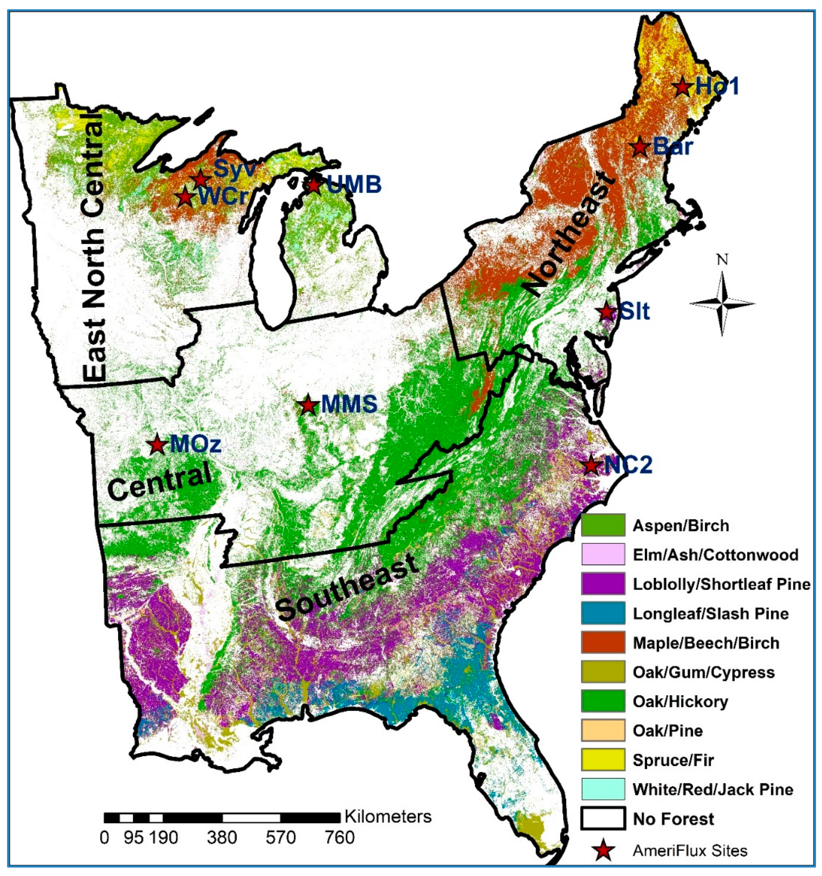
2.1. Study Area Forest Group Type Coverage by Climate Region

The study area for the experimental analysis is the eastern U.S. (Figure 1). The predominant land cover in this region is forest cover consisting of more than 80 tree species [30]. Figure 1 shows the study area and the forest type groups based on the national forest type dataset produced by the United States Forest Service (USFS) Forest Inventory and Analysis (FIA) program and the Remote Sensing Applications Center (RSAC). The national forest type dataset was created by modeling several biophysical layers, including digital elevation models (DEM), Moderate Resolution Spectroradiometer (MODIS) multi-date composites, vegetation indices and vegetation continuous fields, class summaries from the 1992 National Land Cover Dataset (NLCD), various ecologic zones, and summarized PRISM climate data [31]. The national forest types were classified into 28 groups to portray broad distribution patterns of forest cover in the U.S. [30,32]. Our study area includes 10 major forest type groups (Figure 1).

The study area was divided into Central, East North-Central, Northeastern, and Southeastern forest/climate regions [31] (Figure 1). The Oak/Hickory (38%), Loblolly/Shortleaf Pine (17%), and Maple/Beech/Birch (15%) forest type groups dominate the study area. However, each forest/climatic region has its own characteristic and areal extent of forest group types as well as species composition. For example, the highest percent area coverage of the Northeast Climate Region is the Maple/Beech/Birch Group (about 66%), followed by the Oak/Hickory Group (about 22%). In contrast, the highest percent cover of the forest group in the Southeast Climate Region is the Oak/Hickory Group (about 40%), followed by Loblolly/Shortleaf Pine Group (about 28%). Detailed information and the data for the U.S. is available at USDA’s Forest Service website at [31].

2.2. Data Used in ForDRI Model Development

The ForDRI model includes water cycle variables (precipitation, temperature, evaporation, soil moisture, and vapor pressure deficit) that influence short- and long-term drought conditions that are combined with satellite-derived vegetation reflectances (NDVI) that characterize forest condition. The input variables are described in additional detail below.

2.2.1. MODIS-based Normalized Difference Vegetation Index (NDVI)

The normalized difference vegetation index (NDVI) information at 250-meter (m) spatial resolution is based on Moderate Resolution Imaging Spectroradiometer (MODIS) data acquired by the National Aeronautics and Space Administration’s (NASA) Earth Observing System (EOS). The MODIS-based 7-day data from 2003–2017 were acquired from USGS [33] and resampled to a 1 km grid, and each dataset was standardized (Z-score) to be consistent with the other input variables. The Z-score was calculated using the formula: weekly-observed value minus weekly-mean value divided by the standard deviation. This dataset can be accessed at USGS Earth Explorer [33].

2.2.2. Standardized Precipitation Index (SPI)

The SPI was calculated to quantify the precipitation anomaly for three specified time-scales (the previous 12, 24, and 60 months) based on the long-term precipitation record over that specific time interval [12,34]. Since the SPI values are calculated by fitting the long-term record of precipitation over a specific time step to a probability distribution to standardize the values, we have used these three SPI values to represent different time scales of the rainfall conditions that would affect forest health. The three SPIs are selected to represent the long-term precipitation impact (from 1 year to 5 years) on tree stress. The rainfall data used to generate the time series of SPI were obtained from Applied Climate Information System (ACIS) meteorological station data across the study region. We used the available daily long-term record of each station to generate SPI at 12-, 24-, and 60-month aggregate periods and interpolated using the inverse-distance weight (IDW) method to produce 1 km resolution SPI maps.

2.2.3. Standardized Precipitation Evapotranspiration Index (SPEI)

Unlike the SPI, which depends only on rainfall, the SPEI is designed to take into account both precipitation and temperature. The time series of the SPEI were generated based on daily rainfall and temperature data acquired from ACIS meteorological station data. The SPEI were generated at 24- and 60-month aggregate periods and interpolated (using the IDW method) to 12.5 km spatial resolution. With the temperature input, potential evapotranspiration (PET) is calculated and a historical time series of the simple water balance (precipitation—PET) is used in determining drought. Thus, the SPEI captures the main impact of increased temperatures on water demand [35]. Two specified time periods of SPEI historical records (i.e., the previous 24 and 60 months) that represent the temperature impact on water demand (rainfall) were used in building the ForDRI model to monitor forest drought response.

2.2.4. Evaporative Demand Drought Index (EDDI)

The EDDI indicates the anomalous condition of the atmospheric evaporative demand (also known as “the thirst of the atmosphere”) for a given location and across a time period of interest [36,37]. The EDDI is expressed as atmospheric evaporative demand (Eo) anomalies. The Eo is calculated using the Penman–Monteith FAO56 reference evapotranspiration formulation driven by temperature, humidity, wind speed, and incoming solar radiation from the North American Land Data Assimilation System datasets (NLDAS-2). EDDI is multi-scalar (i.e., captures drying dynamics that themselves operate at different timescales). We combined 12-month aggregated EDDI values with the other variables to monitor evaporative demand during forest drought.

2.2.5. Ground Water Storage (GWS)

GWS anomalies are calculated from Gravity Recovery and Climate Experiment (GRACE) observations [38,39]. Data from the Global Land Data Assimilation System (GLDAS), including Terrestrial Water Storage (TWS), Root Zone Soil Moisture (RZSM) at 1-meter depth, and Snow Water Equivalence (SWE), were used to convert GRACE observations into a series of GWS anomalies (i.e., GWS = TWS – RZSM – SWE). NASA provided the data (2003 to 2017) at 12.5 km resolution for the U.S. The ground water product at 1-meter depth represents deeper soil condition that can be accessed by deeper-rooted tree species. The global GRACE data (2003–2020) are also available online from the NASA GSFC Hydrological Sciences Laboratory at the NASA GESDISC data archive [40].

2.2.6. Palmer Drought Severity Index (PDSI) and Palmer Z Index (PZI)

The PDSI has been one of the most widely used climate-based drought indices in the U.S. [41]. The PDSI is calculated based on a simple supply-and-demand model of a water balance equation using historical records of precipitation and temperature as well as available water-holding capacity of the soil at a given location [14,15]. The PDSI is calculated using a combination of current and previous climatic conditions. In contrast to the PDSI, the Palmer Z-Index (PZI) corresponds to monthly drought conditions with no memory of previous monthly deficits or surpluses [14,15]. Thus, in this study, we have used the PDSI and 60-month PZI historical datasets to represent the short- and long-term drought conditions that impact forests.

2.2.7. Noah Soil Moisture (SM)

The Noah soil moisture dataset used in this study is produced using a land surface model that forms a component of the GLDAS [42,43,44]. The Noah soil moisture represents shallow soil depth conditions that can be accessed by shallow-rooted species. Compared to other NLDAS-2 soil moisture products (e.g., VIC), Noah soil moisture shows the best performance in simulating shallow depth soil moisture [45]. The Noah model uses a four-layered soil description with a 10-cm thick top layer and takes into account the fractions of sand and clay. Soil moisture dynamics of the top layer are governed by infiltration, surface and sub-surface runoff, gradient diffusion, gravity, and evapotranspiration [46]. The model was forced by a combination of NOAA/GLDAS atmospheric analysis fields, spatially and temporally disaggregated NOAA Climate Prediction Center Merged Analysis of Precipitation (CMAP) fields, and observation-based downward shortwave and longwave radiation fields derived using a method of the Air Force Weather Agency’s agricultural meteorological system [40]. The historical data (available since 2000) has a 25 km resolution (resampled to 1 km for combining with other model inputs). This dataset is also available as NOAA’s NLDAS Drought Monitor Soil Moisture [47].

2.2.8. Vapor Pressure Deficit

The vapor pressure deficit (VPD) represents the difference between the actual water vapor pressure in the air and the vapor pressure when the air at that temperature is saturated [48]. The VPD is one of the critical variables that control photosynthesis and water use efficiency of plants. The photosynthetic rates in leaves and canopies is inversely proportional to the atmospheric VPD [49]. Thus, it is important for forest ecosystem structure and function [50]. Average daily VPD data using the PRISM model at 4 km resolution were retrieved from the PRISM Climate Group, Oregon State University [51,52,53].

2.2.9. National Forest Groups and Types

The national forest types and forest groups geospatial dataset (1 km spatial resolution) used in this study was created by the USFS Forest Inventory and Analysis (FIA) program and the Remote Sensing Applications Center (RSAC) to show the extent, distribution, and forest type composition of the nation’s forests. The dataset was created by modeling forest type from FIA plot data as a function of more than 100 geospatially continuous predictor layers. This process results in a view of forest type distribution in greater detail than is possible with the FIA plot data alone. The ForDRI model is calculated for forest areas based on this national forest type dataset acquired from the USDA Forest Service [31].

2.2.10. Bowen Ratio Data to Compare with ForDRI at Nine AmeriFlux Sites

Plant water stress is typically characterized by the water potential (ψ), which represents the tension in the water column and reflects the balance of free energy between atmospheric demand and soil water supply, modulated by leaf stomatal and hydraulic resistances [54]. Plant water potentials can be measured via pressure chamber [55] or in-situ hygrometer [56], but long-term observations across a range of sites are not available.

Energy balance considerations mean that net radiation (R_n) at a forest site is balanced by the energy of sensible heat (H) and evaporation (λE) plus any change in storage (S):

$$R_n=H+\mathit{\lambda }E+S$$

(1)

The change in energy storage associated with ground or canopy heat flux is small compared to the other terms and averages over time to zero. Evaporation from a canopy in energy terms (W m⁻²) is described by the Penman–Monteith equation [57]:

$$\mathit{\lambda }E=\frac{\mathsf{\Delta }\left(R_n-S\right)+c_p\rho {\delta }_e{g}_a}{\mathsf{\Delta }+\mathit{\gamma }\left(1+g_a/g_s\right)}$$

(2)

where R_n and S are as above, δ_e is the vapor pressure deficit, g_a and g_s are boundary layer and stomatal conductances to water vapor, and Δ, c_p, ρ, and γ are thermodynamic parameters that are weak functions of temperature. The stomatal conductance, g_s, plays an important but not unique role in limiting λE. If λE is reduced because of a change in conductance, then H (and to a lesser extent, S) will rise because of energy balance considerations. This makes the Bowen ratio (β), defined as H/λE, especially sensitive to changes in conductance. Stomatal conductance in turn is a function of incoming solar radiation, the vapor pressure deficit (δ_e), temperature, (internal) CO₂ concentration, and water stress (ψ) [58,59]. During drought, higher temperatures and increased vapor pressure deficits can combine with soil water stress to severely limit g_s and increase H at the expense of λE.

We assessed forest water stress by using sensible (H) and latent heat (λE, evaporation) flux data measured at AmeriFlux network sites to calculate an integrated Bowen ratio (β_i):

$${\beta }_i=\frac{\sum H}{\sum \mathit{\lambda }E}$$

(3)

Measured 30-minute H and λE fluxes (no gap filled values) were summed over 7 days, when both were >50 W m⁻². The 7-day integration period was chosen to match the weekly timestep of ForDRI. The Bowen ratio in this context thus represents the weekly partitioning of the site net radiation. When a tree canopy is fully developed and water is passing through foliage on its way to the atmosphere, λE is generally greater than H, and β < 1. When water stress occurs, evaporation from a canopy is limited by stomatal closure and potentially, reduced foliage area. These limits result in more of the incoming energy being converted to sensible heat causing the Bowen ratio to increase.

Sensible (H) and latent (λE) heat data from nine forested AmeriFlux eddy covariance sites in the eastern U.S. were used to calculate the weekly Bowen ratio (β_ι). These represented all forested sites in the eastern U.S. with 12 or more years of H and λE data (

Table 1. Characteristics of AmeriFlux sites used in this analysis. DBF indicates deciduous broadleaf forest, ENF indicates evergreen needle-leaf forest, and MF indicates mixed forest. In the Köppen climate classification, Cfa = humid subtropical climate, Dfa = hot-summer humid continental climate, and Dfb = warm-summer humid continental climate.

Site Id	Name	Lat.	Long.	Elev. (m)	Veg.	Climate	MAT (°C)	MAP (mm)	Start	End	Site ref.
US-Bar	Bartlett Experimental Forest	44.065	−71.288	272	DBF	Dfb	5.61	1246	2004	2017	[60]
US-Ho1	Howland Forest (main tower)	45.204	−68.740	60	ENF	Dfb	5.27	1070	1996	2018	[61]
US-MMS	Morgan Monroe State Forest	39.323	−86.413	275	DBF	Cfa	10.85	1032	1999	2020	[6]
US-MOz	Missouri Ozark Site	38.744	−92.2	219	DBF	Cfa	12.11	986	2004	2017	[62]
US-NC2	NC Loblolly Plantation	35.803	−76.669	5	ENF	Cfa	16.6	1320	2005	2019	[63]
US-Slt	Silas Little Forest	39.914	−74.596	30	DBF	Dfa	11.04	1138	2005	2017	[64,65]
US-Syv	Sylvania Wilderness Area	46.242	−89.348	540	MF	Dfb	3.81	826	2001	2020	[66]
US-UMB	Univ. of Mich. Biological Station	45.560	−84.714	234	DBF	Dfb	5.83	803	2000	2019	[67]
US-WCr	Willow Creek	45.806	−90.080	520	DBF	Dfb	4.02	787	1998	2020	[68]

). Because there are seasonal as well as site-to-site variations in β, we normalized weekly, log-transformed integrated Bowen ratios (${\log }_{10}{\beta }_i$) by their standard deviations (σ) from the weekly mean over the full record ($\overline{{\log }_{10}{\beta }_i}$, where a negative value indicates a higher than average β_ι and more drought-stressed conditions). This normalization (also referred to as a Z-score) occurs for each week of the growing season and helps highlight unusual behavior in the weekly β_ι values consistently across sites.

$$Z–score\left({\beta }_i\right)= \frac{\overline{{\log }_{10}{\beta }_{\iota }}-{\log }_{10}{\beta }_i}{\sigma }$$

(4)

This normalization also means that in a long enough record there is a direct, probabilistic interpretation of values based on characteristics of the normal distribution (e.g., a 2σ result has a single-tailed probability of ~2.27%, a 3σ result has p < 0.2%, etc.).

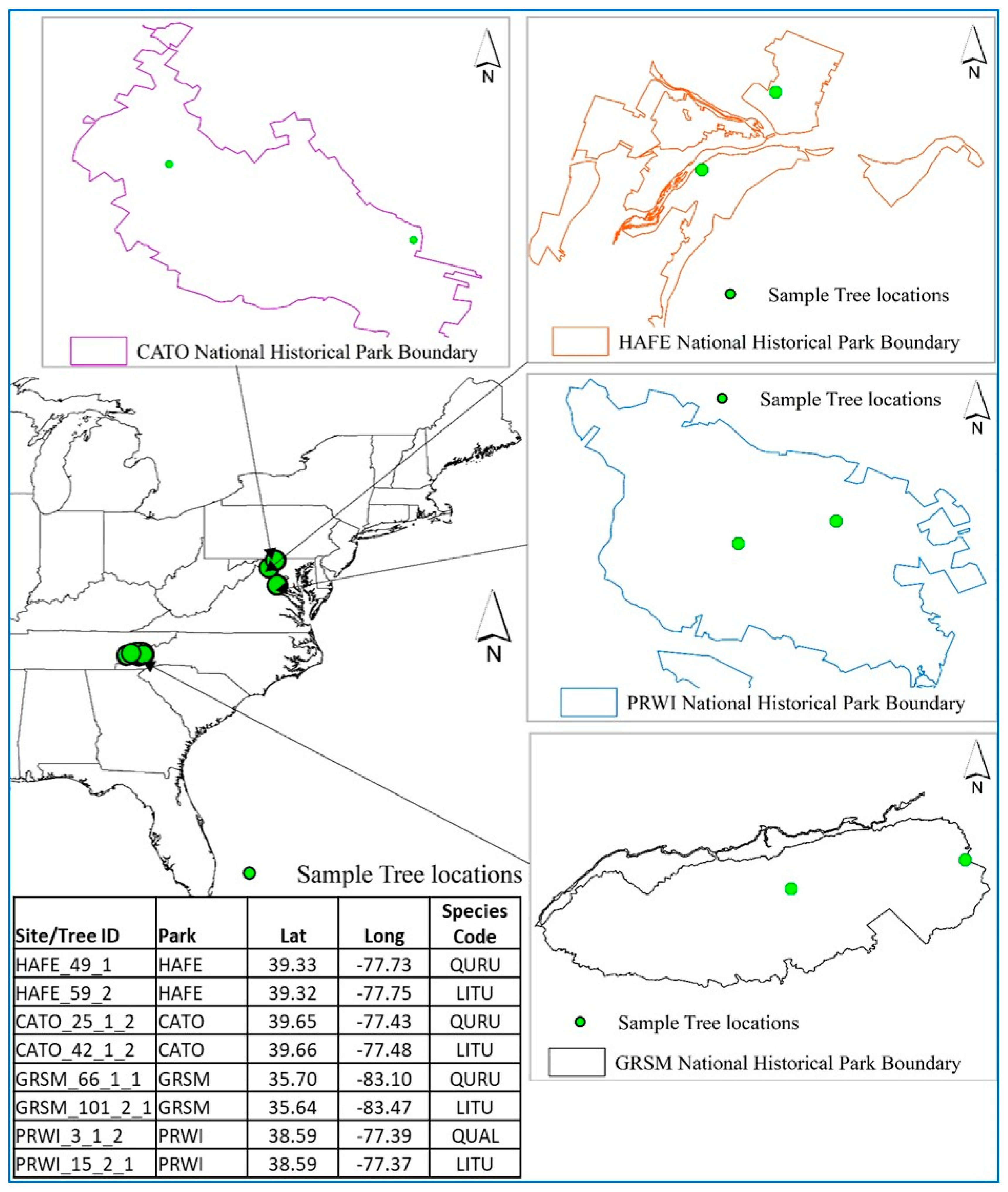
2.2.11. Tree Ring Data for Evaluation

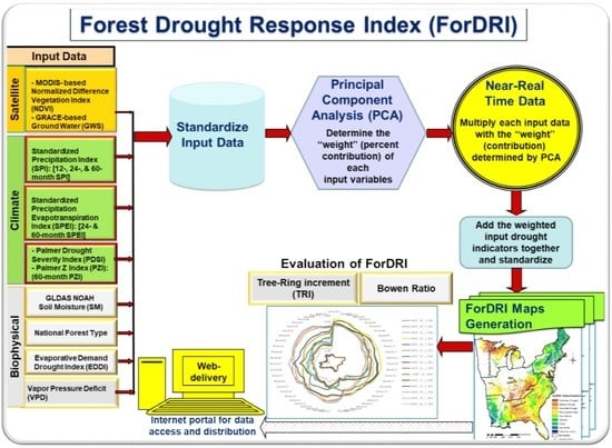
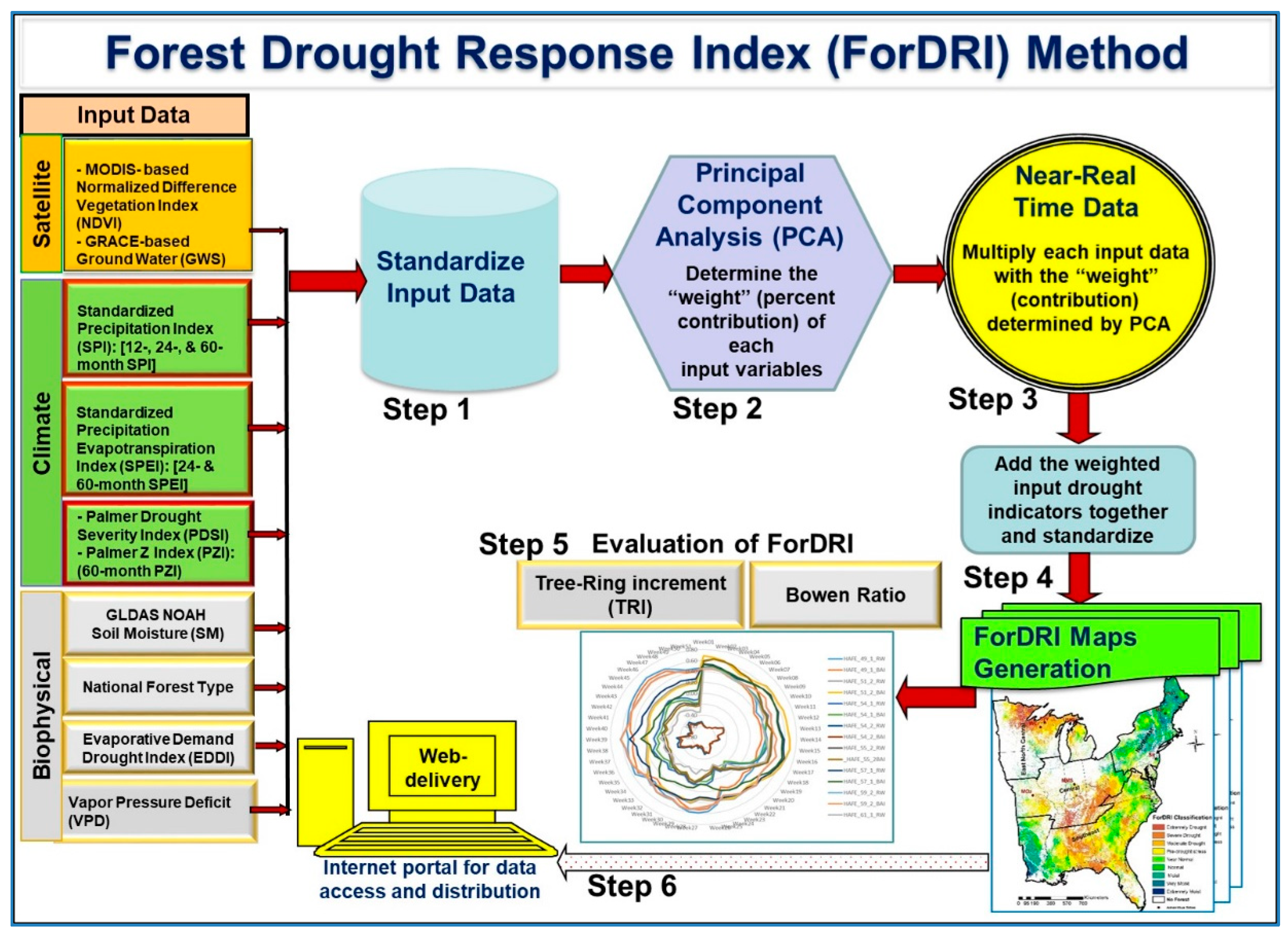
Landsat-based Phenology and Tree Ring data (1984–2013) for Eastern US Forests were acquired for evaluation of ForDRI from the Oak Ridge National Laboratory Distributed Active Archive Center (ORNL DAAC). This dataset provides a 30-year record of forest phenology and annual tree ring data at several selected forested sites in the eastern U.S. [69]. These selected sites are located in four national parks—Harpers Ferry National Historical Park (HAFE), Prince William Forest Park (PRWI), Great Smoky Mountains National Park (GRSM), and Catoctin Mountain Park (CATO). Details of sample preparation and dendrochronological analyses are presented in [70]. We have used eight sites from the four parks (two sites per park) to compare tree ring increment with ForDRI values during the summer season (June to September).

2.3. Methods

2.3.1. ForDRI Model Development

To develop a proof-of-concept ForDRI model, we used 12 selected variables (described above) that contribute to forest drought (Figure 2). The input variables include MODIS-based NDVI, GRACE-based ground water storage, three SPI timescales (12-, 24-, and 60-month SPI), two SPEIs (12- and 24-month SPEI), PDSI, PZI, Noah soil moisture, 12-month EDDI, and VPD. To determine the contribution of each input variables objectively, we have used the principal component analysis (PCA) method. Using the PCA approach, the weights of each variable are determined based on their historical data and the covariance of all input variables (Figure 2; Step 2). This approach helps in limiting the redundant information that could influence the combined ForDRI model. In addition, the PCA-based process is automatic (using scripts), which allows us to produce a separate model for each week in a year using several inputs at a higher spatial resolution [71,72]. Figure 2 shows the method and steps to develop the ForDRI model and the process of producing maps for the forest regions. The process includes six steps from data processing to product dissemination. As shown in Figure 2, the main steps are (i) standardizing all the input variables to be consistent in combining them, (ii) determining the percent contribution (weight) of each input variable based on the covariance of the variables using the PCA method, (iii) multiplying each input variable with the proportion (weight) determined by PCA, (iv) adding the weighted input variables and standardizing the output using long historical records and generating the ForDRI maps for the selected forest regions (we generated the ForDRI maps for the four forest regions of the eastern U.S. to demonstrate and evaluate ForDRI, Figure 3), (v) evaluating the ForDRI maps using tree ring increment (dendrology) data and forest flux data (i.e., Bowen Ratio), and (vi) disseminating the ForDRI maps. In this study, Steps 1 to 5 (Figure 2) were used. For Step 4, the historical data were used in hindsight as “Near-real Time data” to demonstrate the ForDRI model’s capability. The last step (i.e., Step 6, Internet portal for data access and distribution) is the potential delivery of the operational ForDRI maps to the public in the future. An operational ForDRI model is planned to be developed after expanding the model to the western U.S. and evaluating the final national ForDRI model for the continental U.S. (CONUS).

2.3.2. Evaluation Method/Approaches for ForDRI (Both Qualitative and Quantitative Approaches)

For this initial version of the ForDRI model, we used climatic, satellite, and biophysical data for the eastern U.S. (east of 100°W) at a weekly timestep. Forests in the eastern U.S. experience occasional drought, but they tend to be shorter and more random than the seasonal droughts of the West [73]. To evaluate the ForDRI model, we needed long-term measures of forest physiological stress from a variety of sites sufficient to capture a number of significant drought events. As described earlier, our approach was to evaluate ForDRI by assessing forest water stress using sensible and latent heat (evapotranspiration) flux data measured at AmeriFlux network sites to calculate an integrated Bowen ratio and by comparison with estimates of forest growth. It is well known that drought is a primary limit on tree growth and its effects can be seen in tree ring increments [74]. We also evaluated the ForDRI model by qualitatively comparing the spatial patterns and intensity of the drought conditions depicted on the U.S. Drought Monitor (USDM) maps during selected drought years. The USDM is a hybrid product, developed using several sources of ground observation and remote-sensed data including the SPI, PDSI, NDVI, streamflow values, and other drought indicators used by the agriculture, forest, and water management sectors as well as expert feedback from regional and national climatologists.

3. Results

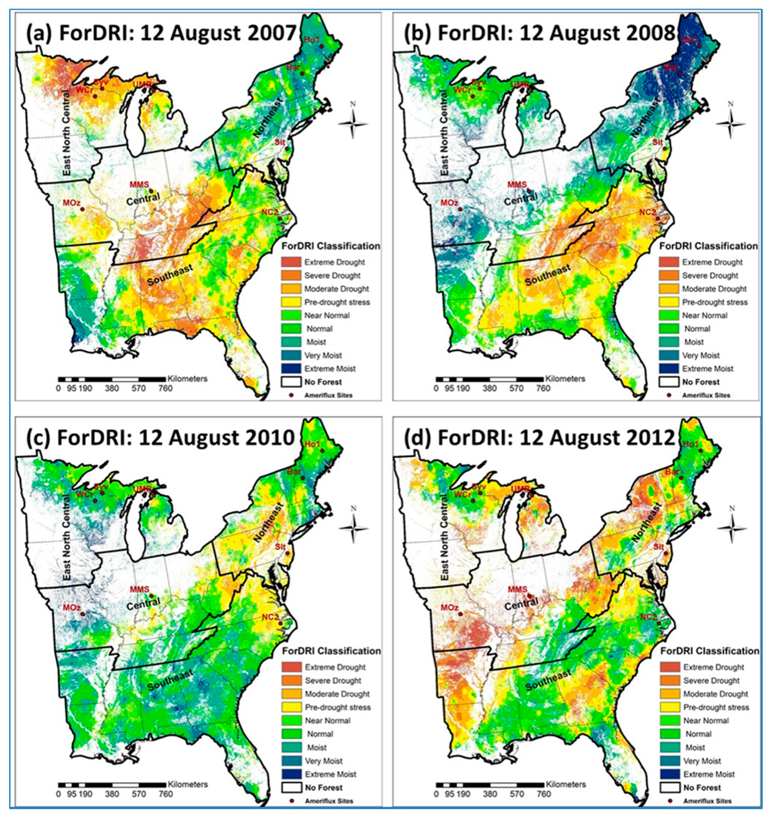
3.1. ForDRI Maps for Selected Drought Years

Historical ForDRI maps (780 maps at a weekly interval) were produced from 2003 to 2017. The same weeks (ending August 12) in 2007, 2008, 2010, and 2012 (Figure 3a–d) are shown below to demonstrate and evaluate the ForDRI model and products. The selection of these drought years was based upon the general long-term drought conditions of the eastern U.S. depicted by the USDM (Figure 4). Even though 2010 was not a drought year over most parts of the U.S., the Northeastern region experienced drought, as shown in Figure 3c.

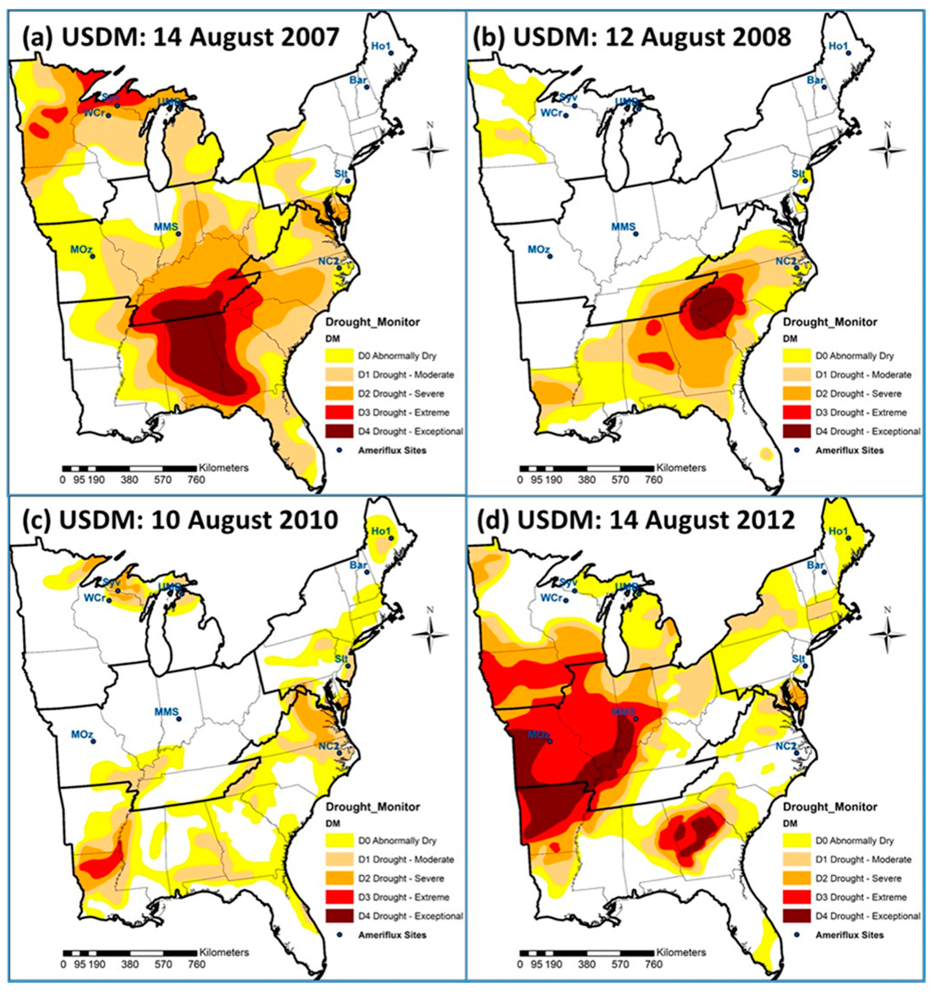
3.2. Comparison of ForDRI with U.S. Drought Monitor (USDM)

The drought intensity estimates of ForDRI broadly agree with those for the same time period produced by the USDM (compare Figure 3; Figure 4). Note that ForDRI masks out non-forested (e.g., agricultural, rangelands, water, and urban) lands that are a focus of the USDM. In mid-August 2007 (Panel “a”), for example, both reach their most severe categories in Alabama-Tennessee and both capture intense drought west of Lake Superior. Details of the patterns differ because of differences in inputs and weighting. In mid-August 2008, for example, ForDRI indicates forest drought stress stretching well into Virginia while the USDM localizes the worst effects in a smaller region (Panel “b”). Both products agree that only mild drought is present in mid-August 2010 (Panel “c”). However, ForDRI does not indicate stress for forests in northern Louisiana while the USDM at that time is indicating short-term (e.g., agricultural) impacts are present. The extreme drought across much of the Midwest in August of 2012 [11] is clearly visible in both products (Figure 3d and Figure 4d).

3.3. Evaluating ForDRI with Bowen Ratio

Figure 5 shows the time-series comparison of the historical records of Bowen Ratio at nine AmeriFlux sites and ForDRI. During the assessment period, two of the flux tower sites, Morgan Monroe (“MMS”, Monroe County, Indiana) and the Missouri Ozarks (“MOz”, Boone County, Missouri) experienced “Exceptional” (D4) drought as defined by the U.S. Drought Monitor (

Table 2. Historic drought at AmeriFlux sites during the ForDRI assessment period based on the U.S. Drought Monitor.

Site	County	State	Year	Dates	Intensity
MMS	Monroe	Indiana	2012	26 June–4 Sept	D2
				17 July–28 Aug	D3
				24 July–7 Aug	D4
			2010	21 Sept–23 November	D2
			2007	21 Aug–26 Oct	D2
MOz	Boone	Missouri
			2012	3 July–end of year	D2
				17 July–16 Oct	D3
				14 Aug–28 Aug	D4
			2006	8 Aug–22 Aug	D2
			2007	21 Aug–16 Oct	D1
NC2	Washington	North Carolina	2011	31 May–23 Aug	D2
				20 Nov–4 Mar 2012	D2
			2008	1 Jan–26 Aug	D2
				29 Jan–12 Feb, 26 Aug (one week)	D3
			2007	4 Sept–23 Oct	D2
Slt	Burlington	New Jersey	2010	7 Sept–28 Sept	D2
			2007	June, Gypsy moth outbreak	none
UMB	Cheboygan	Michigan	2011	29 Mar–26 Apr	D1
			2010	6 April–17 Aug	D1
			2007	28 Aug–4 Sept	D2
			2005	19 July–16 Aug	D2
			2003	7 Jan–1 April, 23 Sept	D1
Syv	Gogebic	Michigan	* 2010	1-29 June	D3
				13 April–17 Aug	D2
			* 2009	22 Sept–20 Oct	D2
			* 2008	26 Aug–12 May 2009	D1
			* 2007	14 Aug–4 Sep	D3
				10 July–16 Oct	D2
			2006	11 July–25 July	D2
WCr	Price	Wisconsin	2012	9–23 Oct	D2
			* 2010	13 April–22 June	D2
			* 2009	4–18 Aug	D3
				25 Jan–Aug	D2
			* 2008	21 Oct–end of year	D2
			* 2007	12–18 Sept	D2
			2005	6 Sept–4 Oct	D2
			2003	18–25 Mar, 22–29 July, 2 Sept–end of year	D1
Ho1	Penobscot	Maine	2016	15 Nov–20 Dec	D2
			2016/17	27 Sept–7 Feb 2017	D1
			2010	10 Aug–28 Sept	D1
Bar	Carrol	New Hampshire	2016/17	27 Sept–7 Feb 2017	D1

* means data not available from flux site for that specific period.

). The North Carolina Pine site (“NC2”, Washington County) experienced “Extreme” (D3) drought, while four sites experienced at least one “Severe” (D2) drought (Table 2). Two sites experienced at most “Moderate” (D1) growing season drought in the period between 2003 and 2017. Both Willow Creek (“WCr”) and the Sylvania Wilderness (“Syv”) sites experienced D3 events in the period between 2007 and 2010 or 2011 when they were offline (no observations available).

The Midwest drought of 2012 is easily seen in the normalized Bowen ratio flux data from both the MMS and MOz sites and is well captured by the ForDRI model (Figure 5). The 2012 drought reached D4 at both sites in August, and both model and data reached a minimum during this event. The normalized Bowen ratio reached −2.89σ at the MOz site and −3.26σ at MMS, consistent with single-tailed probabilities of <1% and <0.1%, indicating the severity of the drought. At both sites, the ForDRI model output is significantly correlated over the entire assessment period with the normalized Bowen ratio data (Z-score β_ι) (p < 0.001, r = 0.56 at Morgan Monroe and r = 0.76 at the Missouri site). A late-summer D2 event at Morgan Monroe in 2010 is also well resolved in both the data and by ForDRI, as is a late summer D1 event in 2007 at both sites. However, a drought classified as D2 by the USDM at the Missouri Ozarks site in 2006 is less clear in the Bowen ratio data and ForDRI model. The ForDRI model and normalized Bowen ratio flux data disagree noticeably at Morgan Monroe in 2014 and at the Missouri Ozarks site in 2015. In both cases, the data suggest ~1σ drier than normal conditions (higher Bowen ratios) while ForDRI indicated wetter than normal. This may be related to tree mortality attributable to 2012 drought that occurred in subsequent years; this delayed effect of drought [62] might complicate the Bowen ratio comparison.

The ForDRI model and Z-score β_ι are also well-correlated (p < 0.001, r = 0.73) at a North Carolina pine forest (NC2) site (Figure 5). The NC2 flux site experienced D2 in the fall of 2007 which worsened to D3 in the spring of 2008. This site also experienced a D2 drought throughout the summer of 2011. All of these events and their relative severity are clearly identified in both ForDRI and the normalized Bowen ratio.

The Silas Little Forest (Slt) in the New Jersey Pine Barrens is characterized by sandy soils with low water holding capacity and drought-tolerant species. The record drought in this time period was September 2010, when the USDM classified Burlington County as D2 for several weeks. The normalized Bowen ratio shows this as a −2σ event and ForDRI identifies it as the most extreme in the interval (Figure 5). However, model and data disagree sharply at this site in the early spring of 2007 when ForDRI was indicating normal moisture conditions while the Z-score β_ι showed this as an extreme stress departure of −2.85σ. ForDRI and the normalized Bowen ratio then came into better agreement as the growing season progressed. The difference can be accounted for by a gypsy moth caterpillar (Lymantria dispar L.) outbreak that removed most foliage from the forest in spring of 2007 [64]. Following the peak of herbivory in mid-June, a second, partial leaf-out occurred and resulted in a canopy with roughly half of the normal summer leaf area [64]. A secondary, lesser defoliation occurred at Silas Little in 2008. With little or no foliage, evaporation was severely constrained, and this resulted in most of the incoming energy being converted to sensible heat and a high Bowen ratio.

ForDRI identified the 2007–2009 drought at Willow Creek and the Sylvania Wilderness that reached D3 when flux data were not available, as well as lesser events. The normalized Bowen ratio data (Z-score β_ι) reached a minimum of −2σ at lesser (D2) events at these sites. However, ForDRI and Z-score β_ι were not significantly correlated at either site over the full data record (Willow Creek, r = 0.10, p = 0.23; Sylvania r = 0.12, p = 0.19). At UMB, the USDM reached D2 in 2005 and 2007, but these periods were poorly resolved by both ForDRI and Z-score β_ι. Both Howland and Bartlett recorded only minor (D1) growing season events during the assessment period, and ForDRI and Z-score β_ι were not significantly correlated at these sites.

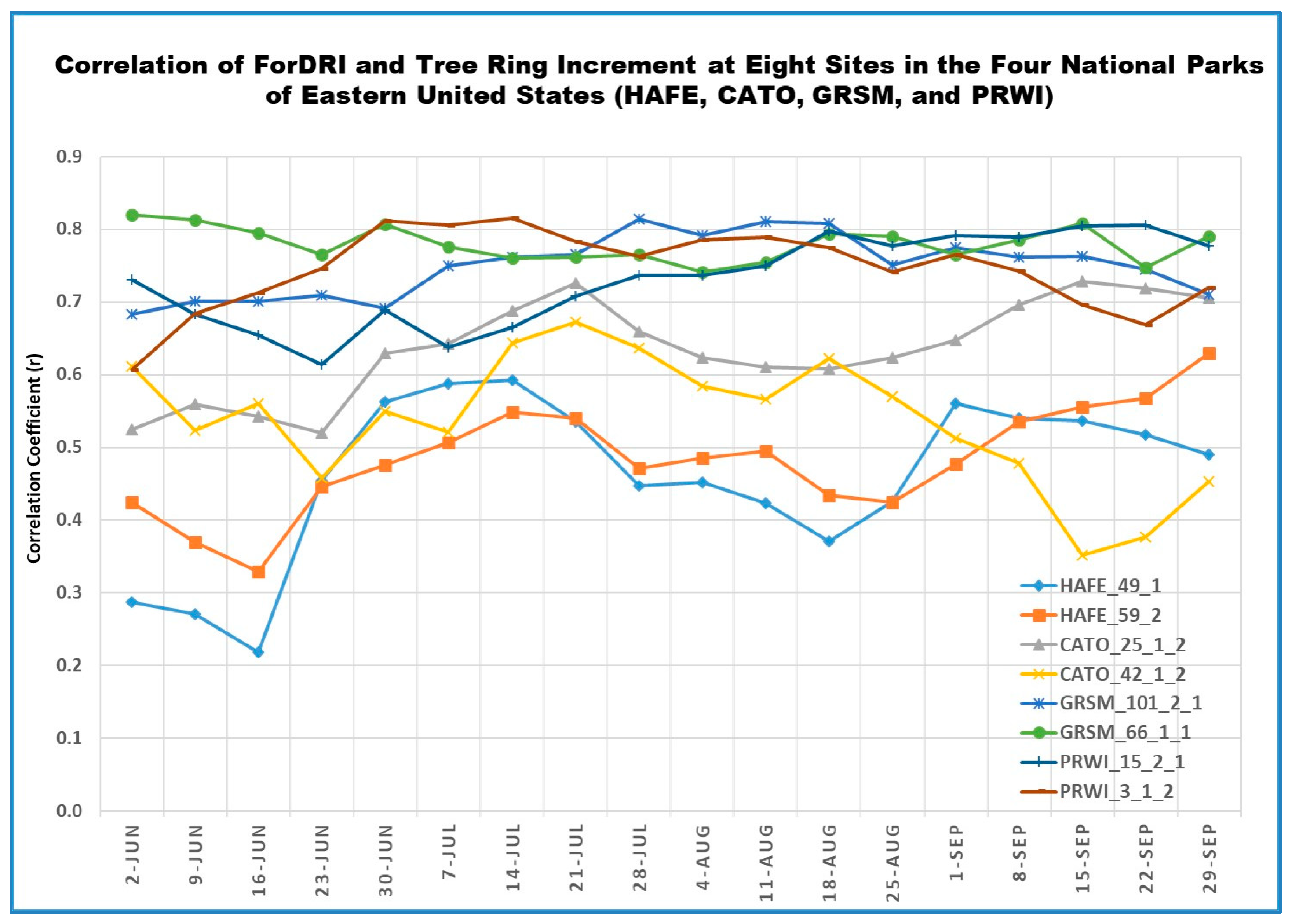
3.4. Evaluating ForDRI with Tree Ring Increments

Tree ring increment (TRI) data from eight sites were used to assess ForDRI values at the four national parks (i.e., HAFE, PRWI, GRSM, and CATO). The tree ring increment is the width of a tree ring that shows the amount of growth taken place over one year and thus indicates the growing conditions for that year. The data that we used include 38 trees in CATO park (two per each site), 115 trees in GRSM (two per each site except one site with only one tree), 24 trees in HAFE (two per each site), and 44 trees in PRWI (two trees per each site). To analyze the correlation of the ForDRI and TRI, two sites from each national park were selected (Figure 6). Three species including American tulip tree (Liriodendron tulipifera), northern red oak (Quercus rubra), and white oak (Quercus alba) were selected for tree ring increment data analysis. Niinemets and Valladares [75] considered Liriodendron tulipifera and Quercus rubra moderately susceptible to drought and Quercus alba moderately tolerant [76]. At each of the selected park sites, the individual tree ID and species type are shown in Figure 6.

Figure 7 shows the correlation between annual tree-ring increment data and ForDRI weekly values during the summer season (June to September). The ForDRI values at a weekly interval were compared with the tree ring annual data at each site between 2003 and 2017 to identify the best period to monitor drought stress on trees using the ForDRI model. The results showed that four sites at GRSM and PRWI have higher correlations (between 0.61 and 0.82) with ForDRI during all weeks of summer (Figure 7) than the other park sites. The correlation peaked when compared with ForDRI values from mid-August. Tree ring increment at the two CATO sites also showed relatively good correlation (0.35 < r < 0.73) with ForDRI. At this site, the highest correlation (0.73) was found in July. Tree ring increments recorded at two HAFE sites showed relatively lower correlations (0.22 < r < 0.63) with ForDRI. This could be because the dominant tree species in the park (oak) are drought-tolerant. In addition, differences in the strength of these relationships may depend upon tree site specifics (ridgetop vs. valley), soils, or other factors. In addition, the frequency and intensity of drought at these four national historic parks over this relatively short interval were not identical. Generally, however, the comparison revealed that the ForDRI values showed reasonable correlation with the tree ring increment, so ForDRI maps may help decision-makers monitor tree drought stress in these parks.

Table 3. Maximum, minimum, and average correlation of ForDRI and tree ring increment (TRI) data at eight sites during summer season (June to September) at four parks in the eastern United States.

Site/Tree ID	Min	Max	Average
HAFE_49_1	0.22	0.59	0.46
HAFE_59_2	0.33	0.63	0.48
CATO_25_1_2	0.52	0.73	0.64
CATO_42_1_2	0.35	0.67	0.54
GRSM_101_2_1	0.68	0.81	0.75
GRSM_66_1_1	0.74	0.82	0.78
PRWI_15_2_1	0.61	0.81	0.73
PRWI_3_1_2	0.61	0.81	0.75

shows the maximum, minimum, and average correlation between ForDRI and tree ring increment data at eight sites of the four national parks in the eastern U.S. during the summer season (June to September). The correlation between ForDRI and tree ring increments at the selected eight sites during summer ranged between 0.46 (minimum) and 0.78 (maximum). The two GRSM sites had higher average correlations (0.75 and 0.78) than the PRWI (0.73 and 0.75), or other sites. Using average summer values of ForDRI accounted for over half the variance in tree ring increment at the GRSM and PRWI sites. Correlations may have been strongest at these two sites because they were impacted by the 2008 Southeast drought (Figure 3b) while the CATO and HAFE sites were not.

4. Discussion

The ForDRI model reaches minimum values at the same times as the normalized Bowen ratio (Z-score of β_ι), a relative measure of physiological water stress. Both of these measures reach minimum values at times when the USDM suggests these forested sites experienced extreme (D3) or exceptional drought (D4). Overall, ForDRI was significantly correlated with the normalized Bowen ratio. At the site level, this correlation was significant at four of the nine sites and can account for over half the variance in the flux-derived quantity. At the sites with lesser (e.g. D2) events in the record, both the normalized Bowen ratio measurements and ForDRI tend to reach at least local minima during the drought event(s) but the correlation between these indicators across the entire time period drops. This lack of correlation at these sites is to be expected when there is little or no drought stress signal to measure. We would expect that other factors such as herbivory and other causes of foliage loss are contributing “noise” to the signals during these non-drought periods and that ForDRI and the normalized Bowen ratio are differentially sensitive to these other factors (the “noise” is uncorrelated). As mentioned earlier, stomatal conductance and β are sensitive to a number of factors in addition to plant (or soil) water stress. These include solar radiation, temperature, and vapor pressure deficit. When significant droughts are absent at a site during the comparison periods (e.g., Bartlett Forest), our normalization scheme will highlight this other variation and magnify disagreement with ForDRI. Bowen ratio data from the Silas Little Forest supports this argument. In 2007, Bowen ratio values at Silas Little Forest reached a minimum, indicating extreme physiological stress, while ForDRI suggested no stress was present. Researchers at the forest, however, report that insects had consumed almost all of the canopy foliage at this time [64]. Without foliage to transpire water, incoming energy was converted to sensible heat and β soared. The stress was real; it just was not caused by drought. Even so, lesser droughts (D2) are easily visible in the normalized Bowen ratio record.

Tree ring increment data were similarly significantly correlated with ForDRI, with higher correlations evident at sites that had experienced more significant drought. The long timespan of developing intense drought (drought serial autocorrelation) was observed in the correlation of annual ring increment with ForDRI estimates across the summer.

A multiyear pattern of drought stress is clearly visible in ForDRI and the normalized Bowen ratio at a number of sites, and critically, in all those that reached D3 or D4. This is an important result as it implies that serious forest drought, the kind that we are most concerned about, takes a long time to develop. It also indicates that ForDRI has a certain capacity to predict the likelihood of extreme (D3) or exceptional drought (D4) prior to, or early in, the growing season. Extreme or exceptional drought conditions seem very unlikely to develop if ForDRI is indicating average or wetter than average conditions at the beginning of the growing season. Conversely, seasons with enhanced likelihood of significant forest drought stress can also be identified. This suggests the possibility of forecasting potential drought maximum severity at the beginning of the growing season, which would be useful to fire managers and many others.

5. Conclusions

We have described ForDRI, a new and non-subjective indicator of forest drought. Weekly values of ForDRI have been calculated since 2003, and in that period, these values readily identify extreme (D3) or exceptional (D4) drought in several research forests. Severe (D2) and less intense droughts are also identified, but at a lower probability of success. A novel and independent measure of forest water stress calculated from forest flux-tower data, weekly, log-transformed integrated Bowen ratios (${\log }_{10}{\beta }_i$) transformed to Z-scores from the weekly mean over the full record, similarly identifies extreme drought periods over the same record. At the sites that have experienced extreme or exceptional drought, these measures are significantly correlated, providing strong evidence for the utility of ForDRI.

The tree ring analysis also showed that the ForDRI values are correlated at the eight sites of the four national parks in the eastern U.S., indicating the drought/water stress impact on tree growth during the drought years. The results showed the potential usefulness of the ForDRI tool for decision making to monitor drought stress on trees in the eastern U.S. and suggest the model can be readily expanded to other parts of the continental U.S.

References

1. Rigden, A.J.; Mueller, N.D.; Holbrook, N.M.; Pillai, N.; Huybers, P. Combined influence of soil moisture and atmospheric evaporative demand is important for accurately predicting US maize yields. Nat. Food 2020, 1, 127–133. [Google Scholar] [CrossRef] [Green Version]
2. Manzoni, S.; Katul, G.; Porporato, A. A dynamical system perspective on plant hydraulic failure. Water Resour. Res. 2014, 50, 5170–5183. [Google Scholar] [CrossRef]
3. Camarero, J.J.; Gazol, A.; Sangüesa-Barreda, G.; Cantero, A.; Sánchez-Salguero, R.; Sánchez-Miranda, A.; Granda, E.; Serra-Maluquer, X.; Ibáñez, R. Forest growth responses to drought at short-and long-term scales in Spain: Squeezing the stress memory from tree rings. Front. Ecol. Evol. 2018, 6, 1–11. [Google Scholar] [CrossRef] [Green Version]
4. Yin, J.; Bauerle, T.L. A global analysis of plant recovery performance from water stress. Oikos 2017, 126, 1377–1388. [Google Scholar] [CrossRef]
5. Matheny, A.M.; Fiorella, R.P.; Bohrer, G.; Poulsen, C.J.; Morin, T.H.; Wunderlich, A.; Vogel, C.S.; Curtis, P.S. Contrasting strategies of hydraulic control in two codominant temperate tree species. Ecohydrology 2017, 10, e1815. [Google Scholar] [CrossRef]
6. Roman, D.T.; Novick, K.A.; Brzostek, E.R.; Dragoni, D.; Rahman, F.; Phillips, R.P. The role of isohydric and anisohydric species in determining ecosystem-scale response to severe drought. Oecologia 2015, 179, 641–654. [Google Scholar] [CrossRef]
7. Plaut, J.A.; Yepez, E.A.; Hill, J.; Pangle, R.; Sperry, J.S.; Pockman, W.T.; Mcdowell, N.G. Hydraulic limits preceding mortality in a piñon–juniper woodland under experimental drought. PlantCell Environ. 2012, 35, 1601–1617. [Google Scholar] [CrossRef]
8. Sanchez-Salguero, R.; Camarero, J.J.; Dobbertin, M.; Fernández-Cancio, A.; Vila-Cabrera, A.; Manzanedo, R.D.; Zavala, M.A.; Navarro-Cerrillo, R.M. Contrasting vulnerability and resilience to drought-induced decline of densely planted vs. natural rear-edge Pinus nigra forests. For. Ecol. Manag. 2013, 310, 956–967. [Google Scholar] [CrossRef]
9. Camarero, J.J.; Gazol, A.; Sanguesa-Barreda, G.; Oliva, J.; Vicente-Serrano, S.M. To die or not to die: Early warnings of tree dieback in response to a severe drought. J. Ecol. 2015, 103, 44–57. [Google Scholar] [CrossRef] [Green Version]
10. Cailleret, M.; Jansen, S.; Robert, E.M.; Desoto, L.; Aakala, T.; Antos, J.A.; Beikircher, B.; Bigler, C.; Bugmann, H.; Caccianiga, M.; et al. A synthesis of radial growth patterns preceding tree mortality. Glob. Chang. Biol. 2017, 23, 1675–1690. [Google Scholar] [CrossRef]
11. Wolf, S.; Keenan, T.F.; Fisher, J.B.; Baldocchi, D.D.; Desai, A.R.; Richardson, A.D.; Scott, R.L.; Law, B.E.; Litvak, M.E.; Brunsell, N.A.; et al. Warm spring reduced carbon cycle impact of the 2012 US summer drought. Proc. Natl. Acad. Sci. USA 2016, 113, 5880–5885. [Google Scholar] [CrossRef] [Green Version]
12. Ruffault, J.; Martin-StPaul, N.; Pimont, F.; Dupuy, J.L. How well do meteorological drought indices predict live fuel moisture content (LFMC)? An assessment for wildfire research and operations in Mediterranean ecosystems. Agric. For. Meteorol. 2018, 262, 391–401. [Google Scholar] [CrossRef]
13. McKee, T.B.; Doesken, N.J.; Kleist, J. Drought Monitoring with Multiple Time Scales. In Proceedings of the 9th Conference on Applied Climatology, Dallas, TX, USA, 15–20 January 1995; American Meteorological Society: Boston, MA, USA. [Google Scholar]
14. Wells, N.; Goddard, S.; Hayes, M.J. A self-calibrating Palmer drought severity index. J. Clim. 2004, 17, 2335–2351. [Google Scholar] [CrossRef]
15. Palmer, W.C. Meteorological Drought; Research Paper, No. 45; US Department of Commerce, Weather Bureau: Washington, DC, USA, 1965; Volume 30, p. 58.
16. Keetch, J.J.; Byram, G.M. A Drought Index for Forest Fire Control; US Department of Agriculture, Forest Service, Southeastern Forest Experiment Station: Asheville, NC, USA, 1968; Volume 38.
17. Koch, F.H.; Smith, W.D.; Coulston, J.W. An improved method for standardized mapping of drought conditions. In Forest Health Monitoring: National Status, Trends, and Analysis 2010. Gen. Tech. Rep. SRS-GTR-176; Potter, K.M., Conkling, B.L., Eds.; US Department of Agriculture, Forest Service, Southern Research Station: Asheville, NC, USA, 2013; pp. 67–83. [Google Scholar]
18. Koch, F.H.; Smith, W.D.; Coulston, J.W. Drought patterns in the conterminous United States and Hawaii. In Forest Health Monitoring: National Status, Trends, and Analysis 2012. Gen. Tech. Rep. SRSGTR-198; Potter, K.M., Conkling, B.L., Eds.; US Department of Agriculture, Forest Service, Southern Research Station: Asheville, NC, USA, 2014; pp. 49–72. [Google Scholar]
19. Koch, F.H.; Smith, W.D.; Coulston, J.W. Drought patterns in the conterminous United States, 2012. In Forest Health Monitoring: National Status, Trends, and Analysis 2013. Gen. Tech. Rep. SRSGTR-207; Potter, K.M., Conkling, B.L., Eds.; US Department of Agriculture, Forest Service, Southern Research Station: Asheville, NC, USA, 2015; pp. 55–69. [Google Scholar]
20. Saleska, S.R.; Didan, K.; Huete, A.R.; da Rocha, H.R. Amazon forests green-up during 2005 drought. Science 2007, 318, 612. [Google Scholar] [CrossRef] [Green Version]
21. Anderson, M.C.; Hain, C.; Wardlow, B.; Pimstein, A.; Mecikalski, J.R.; Kustas, W.P. Evaluation of drought indices based on thermal remote sensing of evapotranspiration over the continental United States. J. Clim. 2011, 24, 2025–2044. [Google Scholar] [CrossRef]
22. Asner, G.P.; Alencar, A. Drought impacts on the Amazon forest: The remote sensing perspective. New Phytol. 2010, 187, 569–578. [Google Scholar] [CrossRef]
23. Pasho, E.; Camarero, J.J.; de Luis, M.; Vicente-Serrano, S.M. Impacts of drought at different time scales on forest growth across a wide climatic gradient in north-eastern Spain. Agric. For. Meteorol. 2011, 151, 1800–1811. [Google Scholar] [CrossRef]
24. Samanta, A.; Ganguly, S.; Myneni, R.B. MODIS enhanced vegetation index data do not show greening of Amazon forests during the 2005 drought. New Phytol. 2011, 189, 11–15. [Google Scholar] [CrossRef] [PubMed]
25. Zhang, Y.; Peng, C.; Li, W.; Fang, X.; Zhang, T.; Zhu, Q.; Chen, H.; Zhao, P. Monitoring and estimating drought-induced impacts on forest structure, growth, function, and ecosystem services using remote-sensing data: Recent progress and future challenges. Environ. Rev. 2013, 21, 103–115. [Google Scholar] [CrossRef]
26. AghaKouchak, A.; Farahmand, A.; Melton, F.S.; Teixeira, J.; Anderson, M.C.; Wardlow, B.D.; Hain, C.R. Remote sensing of drought: Progress, challenges and opportunities. Rev. Geophys. 2015, 53, 452–480. [Google Scholar] [CrossRef] [Green Version]
27. Norman, S.P.; Koch, F.H.; Hargrove, W.W. Review of broad-scale drought monitoring of forests: Toward an integrated data mining approach. For. Ecol. Manag. 2016, 380, 346–358. [Google Scholar] [CrossRef] [Green Version]
28. Svoboda, M.; LeComte, D.; Hayes, M.; Heim, R.; Gleason, K.; Angel, J.; Rippey, B.; Tinker, R.; Palecki, M.; Stooksbury, D.; et al. The drought monitor. Bull. Am. Meteorol. Soc. 2002, 83, 1181–1190. [Google Scholar] [CrossRef] [Green Version]
29. NDMC. U.S. Drought Monitor. 2020. Available online: https://droughtmonitor.unl.edu/About.aspx (accessed on 3 September 2020).
30. Iverson, L.R.; Prasad, A.M. Predicting abundance of 80 tree species following climate change in the eastern United States. Ecol. Monogr. 1998, 68, 465–485. [Google Scholar] [CrossRef]
31. USDA Forest Service. National Forest Type Dataset. 2020. Available online: https://data.fs.usda.gov/geodata/rastergateway/forest_type/ (accessed on 3 September 2020).
32. Ruefenacht, B.; Finco, M.V.; Nelson, M.D.; Czaplewski, R.; Helmer, E.H.; Blackard, J.A.; Holden, G.R.; Lister, A.J.; Salajanu, D.; Weyermann, D.; et al. Conterminous US and Alaska forest type mapping using forest inventory and analysis data. Photogramm. Eng. Remote Sens. 2008, 74, 1379–1388. [Google Scholar] [CrossRef]
33. USGS. EROS Moderate Resolution Imaging Spectroradiometer (eMODIS) Digital Object Identifier (DOI) Number: /10.5066/F7H41PNT). 2020. Available online: https://www.usgs.gov/centers/eros/science/usgs-eros-archive-vegetation-monitoring-eros-moderate-resolution-imaging?qt-science_center_objects=0#qt-science_center_objects (accessed on 3 September 2020).
34. Edwards, D.C.; McKee, T.B. “Characteristics of 20th Century Drought in the United States at Multiple Time Scales,” Climatology Report Number 97-2, Department of Atmospheric Science; Colorado State University: Fort Collins, CO, USA, 1997. [Google Scholar]
35. Vicente-Serrano, S.M.; Beguería, S.; López-Moreno, J.I. A multiscalar drought index sensitive to global warming: The standardized precipitation evapotranspiration index. J. Clim. 2010, 23, 1696–1718. [Google Scholar] [CrossRef] [Green Version]
36. Hobbins, M.T.; Wood, A.; McEvoy, D.J.; Huntington, J.L.; Morton, C.; Anderson, M.; Hain, C. The evaporative demand drought index. Part I: Linking drought evolution to variations in evaporative demand. J. Hydrometeorol. 2016, 17, 1745–1761. [Google Scholar] [CrossRef]
37. McEvoy, D.J.; Huntington, J.L.; Hobbins, M.T.; Wood, A.; Morton, C.; Anderson, M.; Hain, C. The evaporative demand drought index. Part II: CONUS-wide assessment against common drought indicators. J. Hydrometeorol. 2016, 17, 1763–1779. [Google Scholar] [CrossRef]
38. Bhanja, S.N.; Mukherjee, A.; Rodell, M. Groundwater storage change detection from in situ and GRACE-based estimates in major river basins across India. Hydrol. Sci. J. 2020, 65, 650–659. [Google Scholar] [CrossRef]
39. Li, B.; Rodell, M.; Kumar, S.; Beaudoing, H.K.; Getirana, A.; Zaitchik, B.F.; de Goncalves, L.G.; Cossetin, C.; Bhanja, S.; Mukherjee, A.; et al. Global GRACE data assimilation for groundwater and drought monitoring: Advances and challenges. Water Resour. Res. 2019, 55, 7564–7586. [Google Scholar] [CrossRef] [Green Version]
40. NASA GSFC Hydrological Sciences Laboratory—Nasa Gesdisc Data Archive, 2020. Available online: https://hydro1.gesdisc.eosdis.nasa.gov/data/GLDAS/GLDAS_CLSM025_DA1_D.2.2/ (accessed on 3 September 2020).
41. Keyantash, J.; Dracup, J.A. The quantification of drought: An evaluation of drought indices. Bull. Am. Meteorol. Soc. 2002, 83, 1167–1180. [Google Scholar] [CrossRef]
42. Nearing, G.S.; Mocko, D.M.; Peters-Lidard, C.D.; Kumar, S.V.; Xia, Y. Benchmarking NLDAS-2 soil moisture and evapotranspiration to separate uncertainty contributions. J. Hydrometeorol. 2016, 17, 745–759. [Google Scholar] [CrossRef]
43. Xia, Y.; Hao, Z.; Shi, C.; Li, Y.; Meng, J.; Xu, T.; Wu, X.; Zhang, B. Regional and global land data assimilation systems: Innovations, challenges, and prospects. J. Meteorol. Res. 2019, 33, 159–189. [Google Scholar] [CrossRef]
44. Kumar, S.V.; Peters-Lidard, C.D.; Mocko, D.; Reichle, R.; Liu, Y.; Arsenault, K.R.; Xia, Y.; Ek, M.; Riggs, G.; Livneh, B.; et al. Assimilation of remotely sensed soil moisture and snow depth retrievals for drought estimation. J. Hydrometeorol. 2014, 15, 2446–2469. [Google Scholar] [CrossRef]
45. Cai, X.; Yang, Z.L.; Xia, Y.; Huang, M.; Wei, H.; Leung, L.R.; Ek, M.B. Assessment of simulated water balance from Noah, Noah-MP, CLM, and VIC over CONUS using the NLDAS test bed. J. Geophys. Res. Atmos. 2014, 119, 13751–13770. [Google Scholar] [CrossRef]
46. Liu, Y.Y.; Parinussa, R.M.; Dorigo, W.A.; De Jeu, R.A.; Wagner, W.; Van Dijk, A.I.J.M.; McCabe, M.F.; Evans, J.P. Developing an improved soil moisture dataset by blending passive and active microwave satellite-based retrievals. Hydrol. Earth Syst. Sci. 2011, 15, 425–436. [Google Scholar] [CrossRef] [Green Version]
47. NOAA. NLDAS Drought Monitor Soil Moisture. 2020. Available online: https://www.emc.ncep.noaa.gov/mmb/nldas/drought/ (accessed on 3 September 2020).
48. Yuan, W.; Zheng, Y.; Piao, S.; Ciais, P.; Lombardozzi, D.; Wang, Y.; Ryu, Y.; Chen, G.; Dong, W.; Hu, Z.; et al. Increased atmospheric vapor pressure deficit reduces global vegetation growth. Sci. Adv. 2019, 5, eaax1396. [Google Scholar] [CrossRef] [Green Version]
49. Fletcher, A.L.; Sinclair, T.R.; Allen, L.H., Jr. Transpiration responses to vapor pressure deficit in well watered‘slow-wilting’and commercial soybean. Environ. Exp. Bot. 2007, 61, 145–151. [Google Scholar] [CrossRef]
50. Li, P.; Omani, N.; Chaubey, I.; Wei, X. Evaluation of Drought Implications on Ecosystem Services: Freshwater Provisioning and Food Provisioning in the Upper Mississippi River Basin. Int. J. Environ. Res. Public Health 2017, 14, 496. [Google Scholar] [CrossRef] [Green Version]
51. Daly, C.; Halbleib, M.; Smith, J.I.; Gibson, W.P.; Doggett, M.K.; Taylor, G.H.; Curtis, J.; Pasteris, P.A. Physiographically-sensitive mapping of temperature and precipitation across the conterminous United States. Int. J. Climatol. 2008, 28, 2031–2064. [Google Scholar] [CrossRef]
52. Daly, C.; Smith, J.I.; Olson, K.V. Mapping atmospheric moisture climatologies across the conterminous United States. PLoS ONE 2015, 10, e0141140. [Google Scholar] [CrossRef]
53. PRISM Climate Group; Oregon State University. Available online: http://prism.oregonstate.edu (accessed on 1 July 2020).
54. Philip, J.R. Plant water relations: Some physical aspects. Annu. Rev. Plant Physiol. 1966, 17, 245–268. [Google Scholar] [CrossRef]
55. Scholander, P.F.; Bradstreet, E.D.; Hemmingsen, E.A.; Hammel, H.T. Sap pressure in vascular plants: Negative hydrostatic pressure can be measured in plants. Science 1965, 148, 339–346. [Google Scholar] [CrossRef]
56. Baughn, J.W.; Tanner, C.B. Leaf Water Potential: Comparison of Pressure Chamber and in situ Hygrometer on Five Herbaceous Species 1. Crop Sci. 1976, 16, 181–184. [Google Scholar] [CrossRef]
57. Monteith, J.L. Evaporation and Environment. In Symposia of the Society for Experimental Biology 19; Cambridge University Press: Cambridge, UK, 1965; pp. 205–234. [Google Scholar]
58. Jarvis, P.G. The interpretation of the variations in leaf water potential and stomatal conductance found in canopies in the field. Philos. Trans. R. Soc. Lond. B Biol. Sci. 1976, 273, 593–610. [Google Scholar]
59. Cowan, I.R.; Farquhar, G.D. Stomatal function in relation to leaf metabolism and environment. Symp. Soc. Exp. Biol. 1977, 31, 471–505. [Google Scholar]
60. Ouimette, A.P.; Ollinger, S.V.; Richardson, A.D.; Hollinger, D.Y.; Keenan, T.F.; Lepine, L.C.; Vadeboncoeur, M.A. Carbon fluxes and interannual drivers in a temperate forest ecosystem assessed through comparison of top-down and bottom-up approaches. Agric. For. Meteorol. 2018, 256, 420–430. [Google Scholar] [CrossRef] [Green Version]
61. Hollinger, D.Y.; Aber, J.; Dail, B.; Davidson, E.A.; Goltz, S.M.; Hughes, H.; Leclerc, M.Y.; Lee, J.T.; Richardson, A.D.; Rodrigues, C.; et al. Spatial and temporal variability in forest–atmosphere CO2 exchange. Glob. Chang. Biol. 2004, 10, 1689–1706. [Google Scholar] [CrossRef]
62. Gu, L.; Pallardy, S.G.; Hosman, K.P.; Sun, Y. Drought-influenced mortality of tree species with different predawn leaf water dynamics in a decade-long study of a central US forest. Biogeosciences 2015, 12, 2831–2845. [Google Scholar] [CrossRef] [Green Version]
63. Noormets, A.; Gavazzi, M.J.; McNulty, S.G.; Domec, J.C.; Sun, G.E.; King, J.S.; Chen, J. Response of carbon fluxes to drought in a coastal plain loblolly pine forest. Glob. Chang. Biol. 2010, 16, 272–287. [Google Scholar] [CrossRef]
64. Clark, K.L.; Skowronski, N.; Gallagher, M.; Renninger, H.; Schäfer, K. Effects of invasive insects and fire on forest energy exchange and evapotranspiration in the New Jersey pinelands. Agric. For. Meteorol. 2012, 166, 50–61. [Google Scholar] [CrossRef]
65. Clark, K.L.; Renninger, H.J.; Skowronski, N.; Gallagher, M.; Schäfer, K.V. Decadal-scale reduction in forest net ecosystem production following insect defoliation contrasts with short-term impacts of prescribed fires. Forests 2018, 9, 145. [Google Scholar] [CrossRef] [Green Version]
66. Desai, A.R.; Bolstad, P.V.; Cook, B.D.; Davis, K.J.; Carey, E.V. Comparing net ecosystem exchange of carbon dioxide between an old-growth and mature forest in the upper Midwest, USA. Agric. For. Meteorol. 2005, 128, 33–55. [Google Scholar] [CrossRef]
67. Gough, C.M.; Vogel, C.S.; Schmid, H.P.; Su, H.B.; Curtis, P.S. Multi-year convergence of biometric and meteorological estimates of forest carbon storage. Agric. For. Meteorol. 2008, 148, 158–170. [Google Scholar] [CrossRef]
68. Cook, B.D.; Davis, K.J.; Wang, W.; Desai, A.; Berger, B.W.; Teclaw, R.M.; Martin, J.G.; Bolstad, P.V.; Bakwin, P.S.; Yi, C.; et al. Carbon exchange and venting anomalies in an upland deciduous forest in northern Wisconsin, USA. Agric. For. Meteorol. 2004, 126, 271–295. [Google Scholar] [CrossRef]
69. Elmore, A.J.; Nelson, D.; Guinn, S.M.; Paulman, R. Landsat-based Phenology and Tree Ring Characterization, Eastern US Forests, 1984–2013; ORNL DAAC: Oak Ridge, TN, USA, 2017. [CrossRef]
70. Elmore, A.J.; Nelson, D.M.; Craine, J.M. Earlier springs are causing reduced nitrogen availability in North American eastern deciduous forests. Nat. Plants 2016. [Google Scholar] [CrossRef]
71. Kulkarni, S.S.; Wardlow, B.D.; Bayissa, Y.A.; Tadesse, T.; Svoboda, M.D.; Gedam, S.S. Developing a Remote Sensing-Based Combined Drought Indicator Approach for Agricultural Drought Monitoring over Marathwada, India. Remote Sens. 2020, 12, 2091. [Google Scholar] [CrossRef]
72. Bayissa, Y.A.; Tadesse, T.; Svoboda, M.; Wardlow, B.; Poulsen, C.; Swigart, J.; Van Andel, S.J. Developing a satellite-based combined drought indicator to monitor agricultural drought: A case study for Ethiopia. GIscience Remote Sens. 2019, 56, 718–748. [Google Scholar] [CrossRef]
73. Hanson, P.J.; Weltzin, J.F. Drought disturbance from climate change: Response of United States forests. Sci. Total Environ. 2000, 262, 205–220. [Google Scholar] [CrossRef]
74. Fritts, H. Tree Rings and Climate; Elsevier: Amsterdam, The Netherlands, 2012; p. 582. [Google Scholar]
75. Niinemets, Ü.; Valladares, F. Tolerance to shade, drought, and waterlogging of temperate Northern Hemisphere trees and shrubs. Ecol. Monogr. 2006, 76, 521–547. [Google Scholar] [CrossRef]
76. Abrams, M.D. Adaptations and responses to drought in Quercus species of North America. Tree Physiol. 1990, 7, 227–238. [Google Scholar] [CrossRef]
Figure 1. Study area for the Forest Drought Response Index (ForDRI). The map shows the ten major forest group types in the study area based on the USFS National Forest Type dataset [31].
Remotesensing 12 03605 g001
Figure 2. Conceptual method and steps to develop the Forest Drought Response Index (ForDRI).
Remotesensing 12 03605 g002
Figure 3. Example of the Forest Drought Response Index (ForDRI), showing maps of eastern U.S. Forest Service regions for week 32 (August 12) for selected years: (a) 2007, (b) 2008, (c) 2010, and (d) 2012.
Remotesensing 12 03605 g003
Figure 4. The U.S. Drought Monitor (USDM) maps for mid-August: (a) 2007, (b) 2008, (c) 2010, and (d) 2012 for qualitative comparisons.
Remotesensing 12 03605 g004
Figure 5. Comparison of the historical records of ForDRI values and normalized Bowen Ratio (Z-Score βι) at nine AmeriFlux sites that include Bartlett Experimental Forest (Bar), Howland Forest (Ho1), Morgan Monroe State Forest (MMS), Missouri Ozark Site (MOz), North Carolina pine forest (NC2), Silas Little Forest (Slt), Sylvania Wilderness Area (Syv), Univ. of Mich. Biological Station (UMB), and Willow Creek (WCr).
Remotesensing 12 03605 g005
Figure 6. Locations of the tree ring sites and their species types at the selected four national historical parks. The table in the lower left side of the figure shows the species type of each individual tree, indicating the tree species: Quercus alba (QUAL), Liriodendron tulipifera (LITU), and Quercus rubra (QURU).
Remotesensing 12 03605 g006
Figure 7. Time series correlation of ForDRI and tree ring increment data during summer season (June to September) at eight sites across four national parks in the eastern U.S.
Remotesensing 12 03605 g007