Article

Coastal Dam Inundation Assessment for the Yellow River Delta: Measurements, Analysis and Scenario

1
Institute of Estuarine and Coastal Zone, College of Marine Geosciences, Key Lab of Submarine Geosciences and Prospecting Technology, Ministry of Education, Ocean University of China, Qingdao 266100, China
2
Laboratory of Marine Geology, Qingdao National Laboratory for Marine Science and Technology, Qingdao 266061, China
3
State Key Laboratory of Estuarine and Coastal Research, East China Normal University, Shanghai 200062, China
4
College of Geological Engineering and Geomatics, Chang’an University, Xi’an 710054, China
*
Author to whom correspondence should be addressed.
Remote Sens. 2020, 12(21), 3658; https://0-doi-org.brum.beds.ac.uk/10.3390/rs12213658
Submission received: 3 October 2020 / Revised: 3 November 2020 / Accepted: 5 November 2020 / Published: 8 November 2020
(This article belongs to the Special Issue Dam Stability Monitoring with Satellite Geodesy)

Abstract

:
Coastal dams along the Yellow River Delta are built to prevent seawater intrusion. However, land subsidence caused by significant oil, gas and brine extraction, as well as sediment compaction, could exacerbate the flooding effects of sea-level rise and storm surge. In order to evaluate the coastal dam vulnerability, we combined unmanned aerial vehicle (UAV) Light Detection and Ranging (LiDAR) with small baseline subsets (SBAS) interferometric synthetic aperture radar (InSAR) results to generate an accurate coastal dam digital elevation model (DEM) over the next 10, 30 and 80 years. Sea-level simulation was derived from the relative sea-level rise scenarios published by the Intergovernmental Panel on Climate Change (IPCC) and local long-term tide gauge records. Assuming that the current rate of dam vertical deformation and sea-level rise are linear, we then generated different inundation scenarios by the superposition of DEMs and sea-levels at different periods by way of a bathtub model. We found that the overtopping event would likely occur around Year 2050, and the northern part of the dam would lose its protective capability almost entirely by the end of this century. This article provides an alternative cost-effective method for the detection, extraction and monitoring of coastal artificial infrastructure.

Graphical Abstract

1. Introduction

An important industrial zone in China for oil and gas exploration, salt production, aquaculture, etc., the modern Yellow River Delta (YRD; Figure 1a) is located in the Xianhe Town, Dongying City, Shandong Province, covers an area of at least 10,000 km2 and supports more than six million people [1,2]. The Gudong Oilfield is located in the northern delta region of the Yellow River, and is part of China’s second largest oilfield, the Shengli Oilfield [1]. Gudong coastal dam (Figure 1b), with a length of 12 km, was built in the 1980s to prevent the intrusion of seawater and provide the only protection of the oilfield, thus, representing the most important security barrier between the Gudong Oilfield and the Bohai Sea. Gudong oilfield is low-lying with large areas of elevation lying even lower than average sea-level. This is especially important since there is no wetlands or dunes as the buffer of oilfield. [3,4].
In terms of geological conditions, Gudong oilfield located in the northeast of Zhanhua Sag at the Jiyang Depression, and at the southern end of the drape structure of Zhuangxi-Gudong‘s buried mountain drape structural belt [5,6,7,8]. It is a large-scale packaged draping anticline structure oilfield and was the first coastal oilfield developed in the Shengli Oilfield Region. The Gudong Oilfield was discovered in July 1984 and put into full development in May 1986. This oilfield is different from other mining areas, due to its special geological environment, it is under the threats of ground deformation caused by underground resources exploitation, sea-level rise and storm surge all the time.
There exist a significant number of publications evaluating serious ground subsidence caused by the over-exploitation of underground resources and increasing human activity over large river deltas [1,9,10,11,12,13,14,15]. Due to its special geological setting, the oilfield and its affiliated facilities are vulnerable to the threat of land deformation [16]. Figure 2 shows cracks caused by dam deformation. At the same time, rising sea-levels caused by climate change has led to an increase in the frequency and destructiveness of marine disasters [17]. The fragile structure of the retaining wall would be destroyed easily if subjected to a serious marine disaster, such as the damage caused by a typhoon. Figure 3 shows the destruction of Gudong Dam by Super Typhoon Lekima in August 2019. The government invests heavily in flood prevention every year [18,19,20,21], especially within the coastal zone. Therefore, inundation assessment is an important activity in terms of flood control and can aid policy makers in their formulation of reasonable measures to minimize economic losses [20,22].
As a result of the overwhelming damage caused by inundation, many studies related to inundation assessment of coastal areas exist [23,24,25]. These studies can be roughly divided into two categories: the first is the inundation assessment of a fixed land surface with a changing sea-level [17,22,26,27,28,29,30], which is suitable for some stable coasts; the second is the inundation assessment of a changing land surface with a changing sea-level [16,21,31,32,33,34,35,36,37,38], which is suitable for some delta regions.
The digital elevation model (DEM) is one of the most fundamental datasets for inundation analysis. Many previous studies used the publicly released free DEMs, such as the Shuttle Radar Topography Mission (SRTM) [31,39] or ALOS World 3D-30 m (AW3D30), but the accuracy of these DEMs often varies, making them unreliable for sophisticated analysis to some extent [31,35,39,40,41,42]. High precision DEMs can be derived from three different approaches: photogrammetry, interferometric synthetic aperture radar (InSAR), and Light Detection and Ranging (LiDAR) [43]. Gesch, et al. [41] used photogrammetry to obtain the meter-scale DEM of Majuro. The InSAR technique can also been used to obtain DEMs, such as the TanDEM-X DEM from the German Aerospace Center (DLR), which is particularly useful in generating global high-resolution seamless DEMs [43,44,45]. However, the global DEMs available cannot meet the requirement of fine artificial buildings in terms of accuracy and spatial resolution [46]. The airborne LiDAR scanning system can flexibly and precisely obtain high-density 3D point cloud data of the ground and generate digital surface models (DSM) and digital terrain models (DTM) simultaneously, through multiple echo filtering, classification and modelling; this has been widely used in active fault identification, landslide monitoring and coastal zone vulnerability analysis [30,35,40,47].
Many researchers have acknowledged that land surface deformation is a fundamental impact factor that cannot be ignored during inundation assessment of the delta [16,33,34]. As such, it is necessary to simulate DEMs at different time points according to the vertical land deformation rate. As a man-made structure, Gudong Dam suffers the threat of deformation too, as shown in Figure 2. Deformation could be caused by a variety of factors, such as oil and gas exploitation, brine extraction and sediment compaction, which are all common activities in the Yellow River Delta [1,48]. In addition to destroying the structure of the dam, land subsidence can also increase the risk of flooding. Whilst the deformation rate can be obtained by means of the Global Navigation Satellite System (GNSS), leveling and time series InSAR (TS InSAR) [32,49,50]. GNSS and leveling measurements are usually very labor-intensive and so are not suitable for large-scale deformation monitoring with high spatial resolution. Compared to GNSS and leveling measurements, TS InSAR offers a convenient alternative in terms of spatial resolution and economic cost [51].
In the field of inundation assessment, sea-level change is one of the most frequently considered factors. A number of studies focus on the submerged range [52], economic losses [18,20,33] or destruction of the natural environment [3,22] caused by sea-level rise (SLR). The rising sea-level could flood coastal lowlands of China, such as the Bohai Bay, the Yangtze River delta, and the Pearl River delta, which are the most economically and socially developed regions. As the elevations of these areas are generally lower than five meters, SLR represents a huge potential threat in terms of increased coastal tide levels, shortened recurrence patterns of extreme water levels, and enhanced effects of tides and waves [53,54]. This has led to a weakening in the protective function of engineering facilities such as coastal embankments and ports, whilst these increasingly vulnerable facilities cost ever more to maintenance. Moreover, SLR has exacerbated the severity of marine disasters such as storm surges, coastal erosion, floods, salty tides, seawater intrusion and soil salinisation.
Extreme weather is more abrupt and violent than SLR and land deformation, leading to the severe impairment of coastal dams. On 10–12 August 2019, Typhoon Lekima caused significant damage to parts of the retaining walls of Gudong Dam. In other words, even under the protection of the dam, wind and waves could push enormous seawater into the oilfield. A commonly applied concept when simulating extreme weather is the “return period”. However, the water level value from the “return period” is usually fixed and the observation accuracy is low [55].
A review of the existing literature yields few studies focused on slender artificial coastal dam inundation assessment in China [56,57,58]. Therefore, in this study we firstly introduce a combination of measurements from the UAV LiDAR DEM, vertical dam deformation rate from small baseline subsets (SBAS) InSAR, and sea-level simulation applied to different future sea-level rise scenarios. High precision DEMs over the Gudong dam was generated through point cloud data collected by unmanned aerial vehicle (UAV) LiDAR in August 2019. Then we provide a detailed future DEM and sea-level simulation analysis method to generate inundation maps of Gudong Dam at different scenarios, through the integration of multiple measurements from LiDAR DEM, land deformation, sea-level rise, tidal data and storm surge. Furthermore, we evaluate the protection capability of the dam in an intuitive way.

2. Datasets and Methods

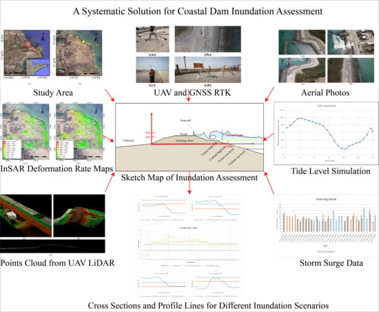
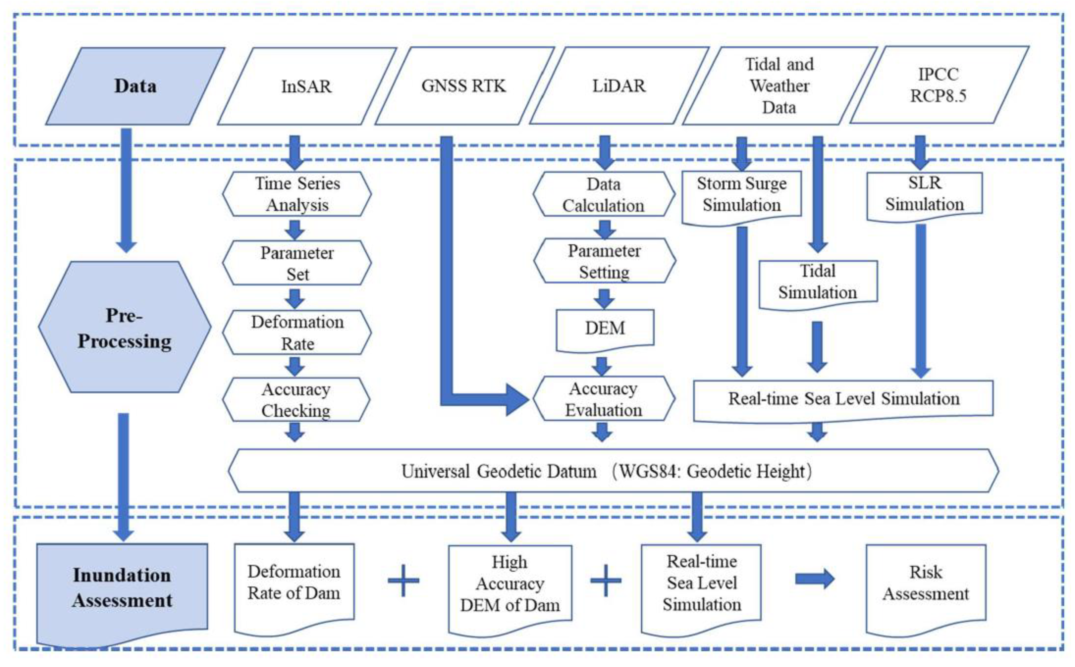
2.1. Flow Chart of Datasets and Methods

Figure 4 is a flow chart of the research methods and datasets that employed in this paper. Details are as follows:
I. Data preparation
  • Sentinel-1 images are utilised to calculate the land surface deformation rate of the coastal dam using SBAS InSAR;
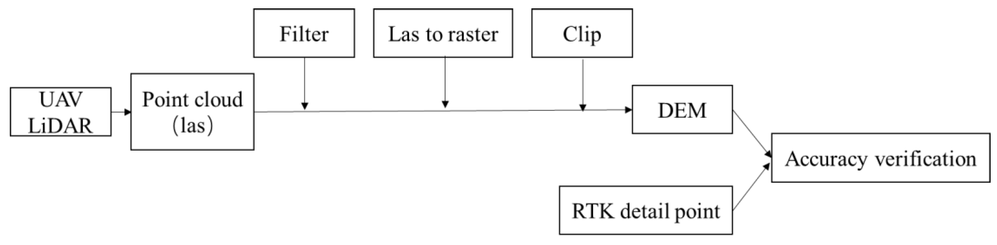
  • Point cloud data of the dam are collected by UAV LiDAR and used to obtain high resolution DEMs;
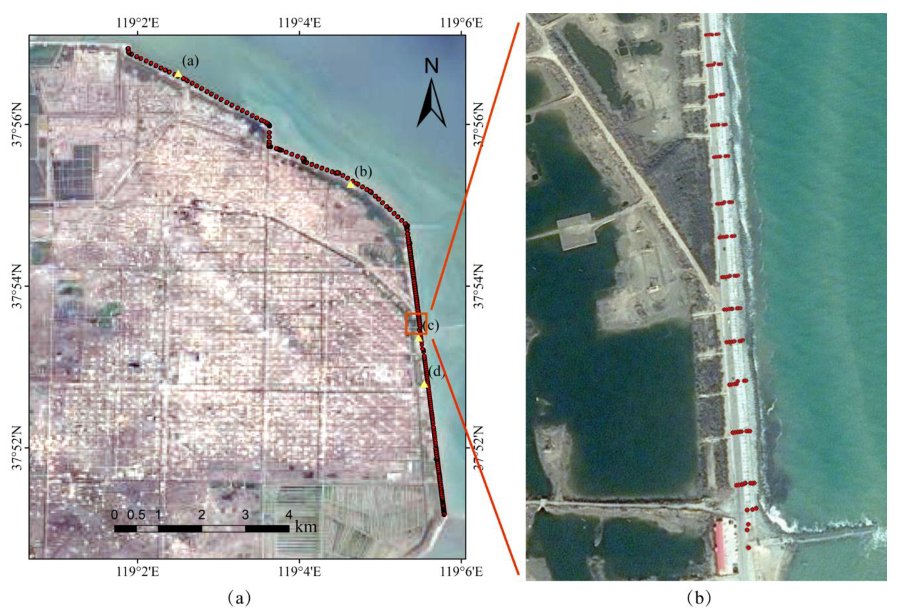
  • Detail points of the dam which are collected using the GNSS real time kinematic (RTK) method are employed to evaluate the accuracy of the DEM;
  • Tide and storm surge records are used to simulate sea-level;
  • The Representative Concentration Pathway 8.5 (RCP8.5) scenario released by the Intergovernmental Panel on Climate Change (IPCC) is used to predict sea-level rise [59].
II. Pre-processing
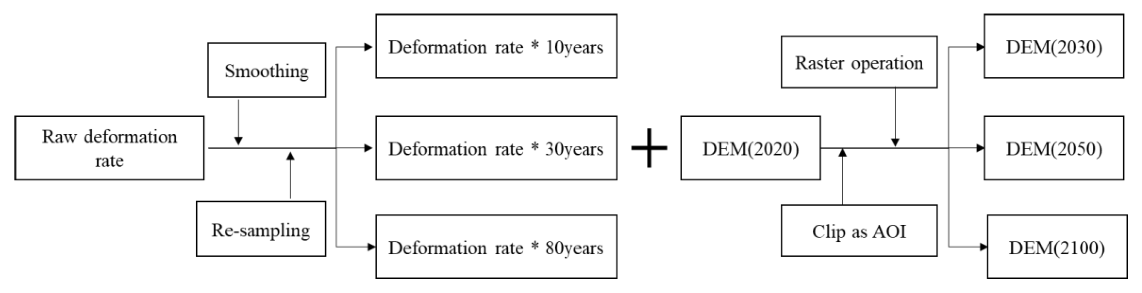
  • Deformation rate is calculated using SBAS InSAR;
  • DEM is simulated using ArcGIS;
  • Sea-level is simulated using Python.
III. Inundation assessment
  • Integration of all the above datasets to simulate flooding scenarios.

2.2. DEM Acquisition and Accuracy Evaluation

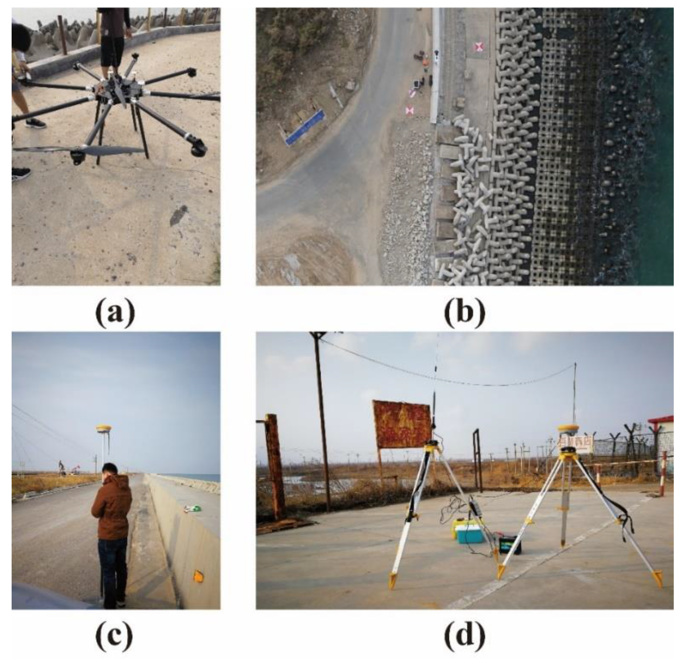
2.2.1. Data Acquisition

Gudong Dam is a slender strip measuring approximately 100 m wide and 12 km long. The DEM of the coastal dam is generated from the point cloud obtained by the UAV LiDAR, applying the Riegl VUX-1 model. Figure 5 sets out UAV and GNSS field measurements and photos of the coastal dam after Super Typhoon Lekima. The point cloud data we used here provides almost full coverage of the dam (Figure 6), but shaded areas containing some missing points are compensated by way of the bilinear interpolation algorithm.

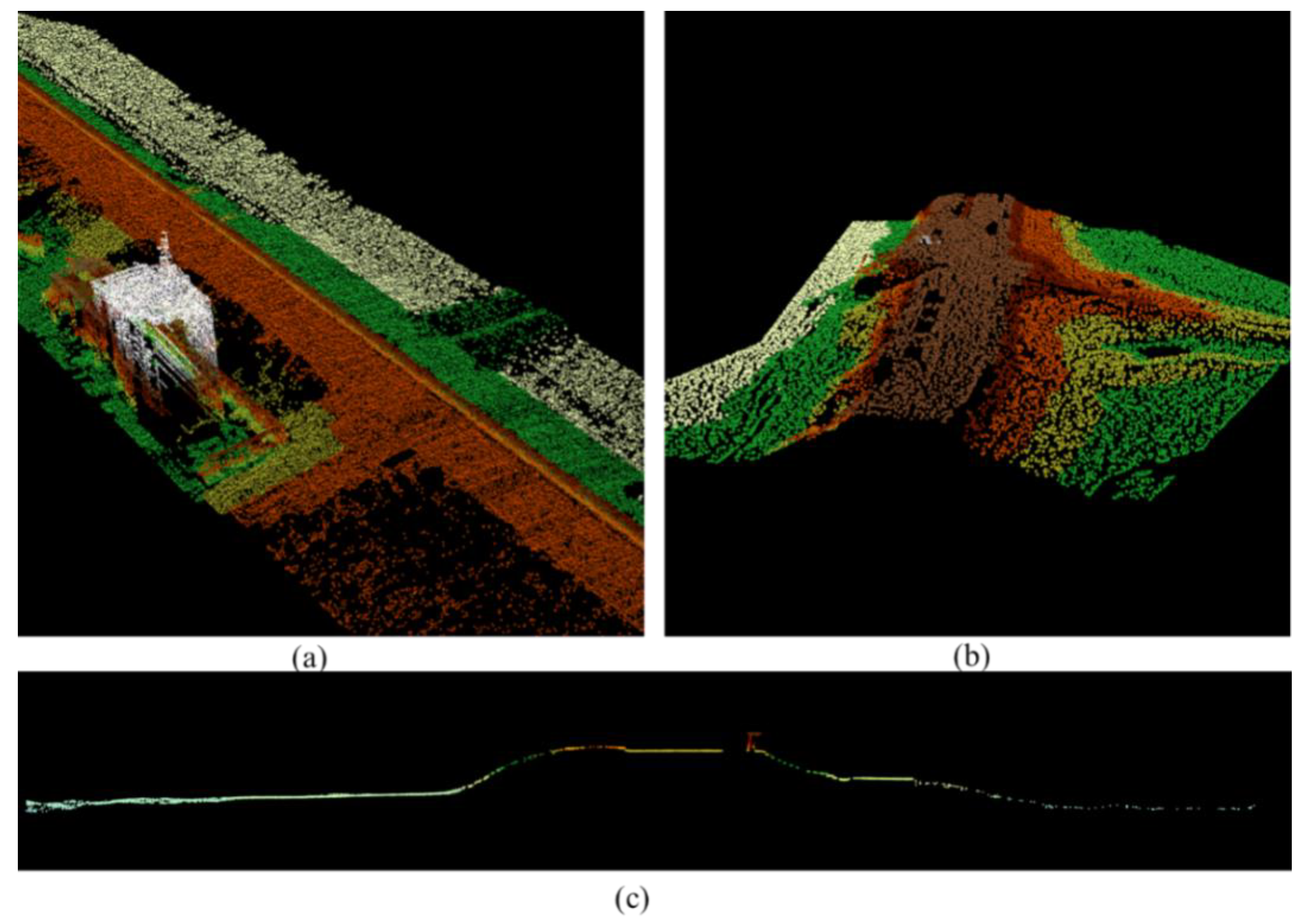
2.2.2. Data Processing and DEM Production

As shown in the flow chart in Figure 7, a point cloud was generated from the raw data collected by UAV LiDAR through data conversion and geo-registration. Necessary processing (such as filtering, laser (LAS) dataset to raster and clipping) was then performed on the point cloud in order to obtain the final DEM over the coastal dam. Its vertical accuracy was evaluated using GNSS RTK measurements. The DEM was used as an important input parameter for the inundation assessment after accuracy verification.
Table 1 shows the main parameters of the DEM generation. We selectively filtered the point cloud to obtain the smooth surface of the dam; that is, all vegetation, buildings, telephone poles, retaining walls and other noise were already removed. Then, we generated the DEM of Gudong Dam at a resolution of 20 * 20 cm using ArcGIS. The DEM generated by the point cloud offered a good level of smoothness and an excellent restoration of the surface of Gudong Dam. Figure 8 illustrates the overall DEM of Gudong Dam.

2.2.3. Accuracy Evaluation of the LiDAR DEM

We collected 1846 accurate GNSS ground measurement points (Figure 9) in January 2020 to evaluate the accuracy of LiDAR DEM. A reference station was set up at a known control point (Figure 5d). Taking into account the error of the temporary control point and the error of GNSS and RTK technology, the estimated accuracy at inner coincidence of the GNSS RTK detail points is about 5 cm.
As a result of outliers or non-normality of the error distribution due to, e.g., filtering and interpolation errors for DEMs derived by laser scanning in non-open terrain, both traditional and robust accuracy measures including mean error (ME), standard deviation (STD), root mean square error (RMS), median, normalized median absolute deviation, 90% linear error (LE90) and correlation are used for the assessment of DEM accuracy [58,60]. The error statistics formulas are listed below.
ME = 1 N i = 1 N ( x i y i ) = 1 N i = 1 N Δ h i
STD = 1 N 1 i = 1 N ( Δ h i M E ) 2
RMS = 1 N i = 1 N Δ h i 2
Q ^ Δ h ( 0.5 ) = m Δ h
M A D = m e d i a n j ( | Δ h j m Δ h | )
N M A D = 1.4826 × m e d i a n j ( | Δ h j m Δ h | )
L E 90 = Q ^ | Δ h | ( 0.9 )
C ( x , y ) =   N x i y i x i y i N x i 2 ( x i ) 2 N y i 2 ( y i ) 2
where x is the elevation collected by the GNSS RTK measurements and y is the elevation of the DEM. The abbreviations of Q∆h(0.5), MAD, NMAD and LE90 indicate the median (50% quantile), the median absolute deviation, the normalized median and the absolute deviation at the 90% quantile, respectively.
As depicted in Figure 10, an excellent correlation of 0.95 was observed between the LiDAR DEM and GNSS heights. A mean difference of −0.05 m and an RMSE value of 0.26 m were obtained from this analysis. The above results are generated without eliminating gross errors (3* RMS) [60]. To resist potential gross errors and outliers, median (0.04 m) and LE90 (0.15 m) values are also calculated. Therefore, we believe that the DEM has good relative accuracy and consistency, and hence, can be used in further analysis.

2.3. Acquisition of Deformation Rate
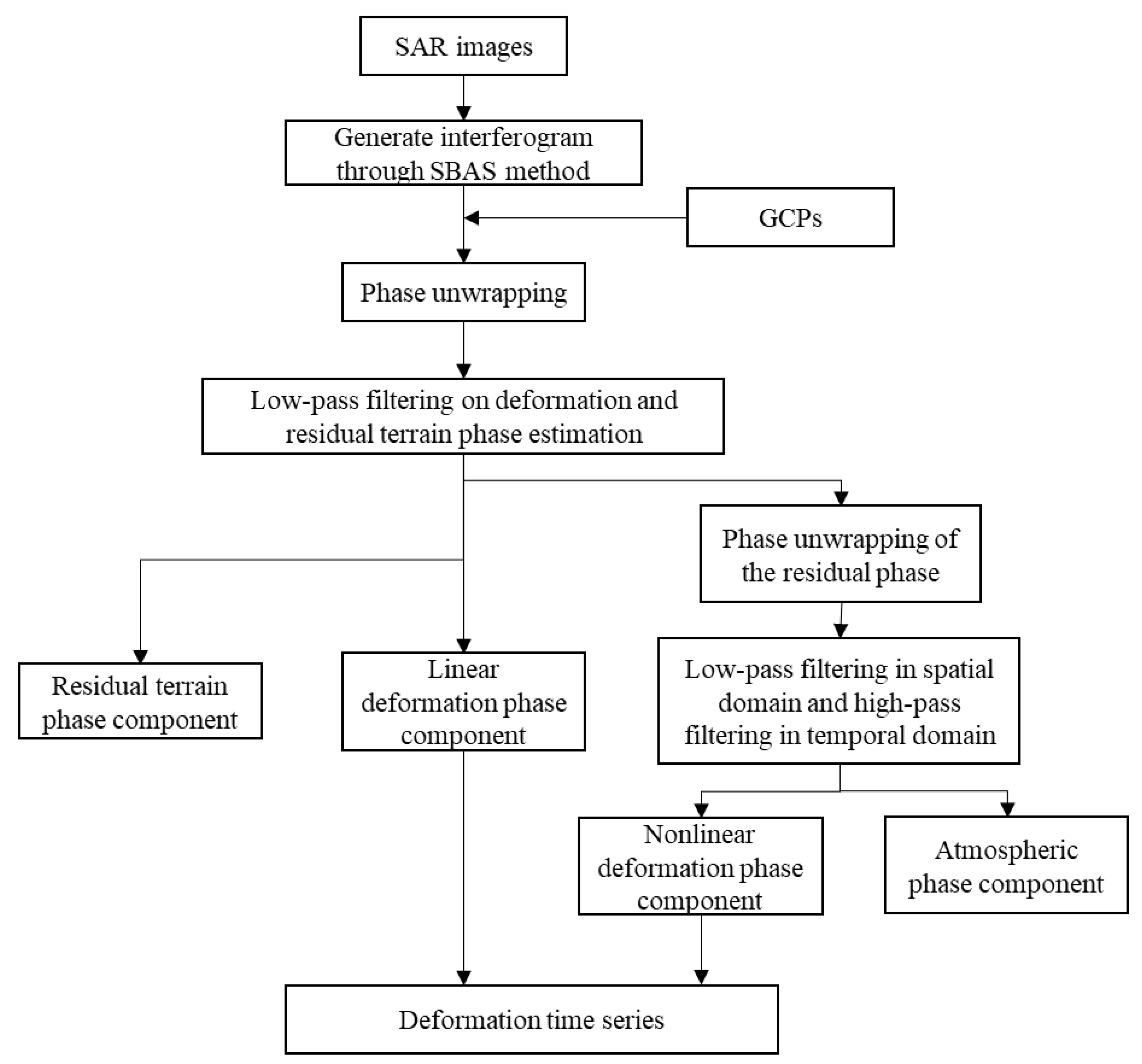
2.3.1. SBAS InSAR

The InSAR technique has been widely used in land deformation monitoring for about 20 years. Advanced InSAR time series analysis—e.g., permanent scatterer (PS) and small baseline subsets (SBAS) approaches—have been developed to overcome InSAR major error sources, including temporal and geometry decorrelation and atmospheric effects [5,61,62,63]. The basic idea of SBAS InSAR is to form those interferograms that meet the conditions of small temporal and spatial baselines into interferometric pairs, which is the limitation of the decorrelation phenomena. Application of the singular value decomposition (SVD) method allows us to easily link independent SAR acquisition datasets which are separated by large baselines, thus, increasing the observation temporal sampling rate. The availability of both spatial and temporal information in the processed data is used to identify and filter out atmospheric phase artifacts [61]. Figure 11 is a flow chart of SBAS InSAR, which has been successfully used to carry out time series deformation on the Naples and Flegrei volcanoes in Italy and the Las Vegas area with high accuracy and reliability [61]. The ground control points (GCPs) in Figure 11 are relatively stable points that will be used as references for phase unwrapping.

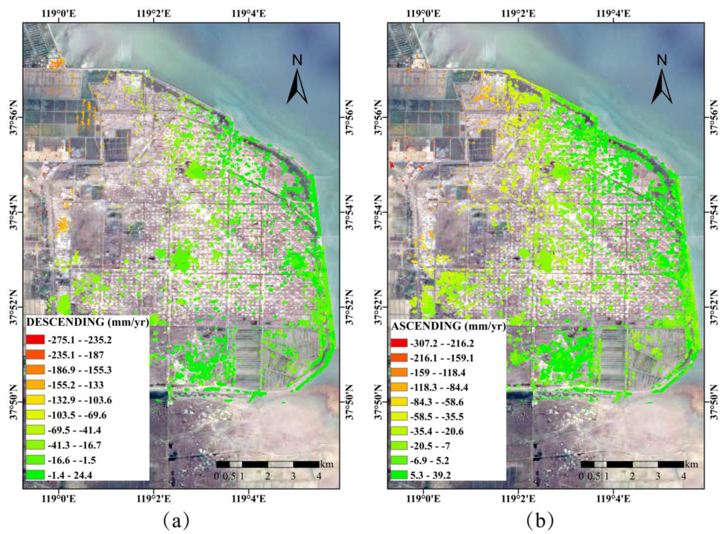
2.3.2. Deformation Rate Acquisition

Considering the disadvantages of traditional measurement methods in spatial resolution and economic cost, SBAS InSAR is capable of quickly obtaining the deformation rate of the study area over a wide range with high accuracy and can aid in locating the deformation center and undertake causal analysis [61,63,64]. Over the last two years, some researchers have utilized TS InSAR techniques to investigate deformation patterning over the Yellow River Delta, but few studies have focused on the engineering stability and vulnerability of a local coastal dam [1,5,6,7,8,10].
As widespread water accumulation and weeds in oilfields lead to a lack of permanent scatterers, we used the SBAS method with ENVI SARscape software to obtain the deformation rate of Gudong Oilfield between 10/2016–07/2019 with Sentinel-1 SAR images. The process flow chart is shown in Figure 11, and the parameters are listed in Table 2. Both ascending (ASC) and descending (DES) tracks of SAR images covering the same time interval were processed, in order to compare and evaluate the results. Figure 12 is the deformation rate map for both ascending and descending orbits. The spatial resolution of the two deformation maps are 20 m * 20 m. Take into account the geological and structural background of the Yellow River Delta, it is assumed that the horizontal deformation is negligible. Therefore, InSAR deformation results from the line of sight (LOS) direction can be calculated with the following equation:
d v e r t i c a l = d L O S cos θ
where θ is incidence angle and d is the InSAR deformation rate.

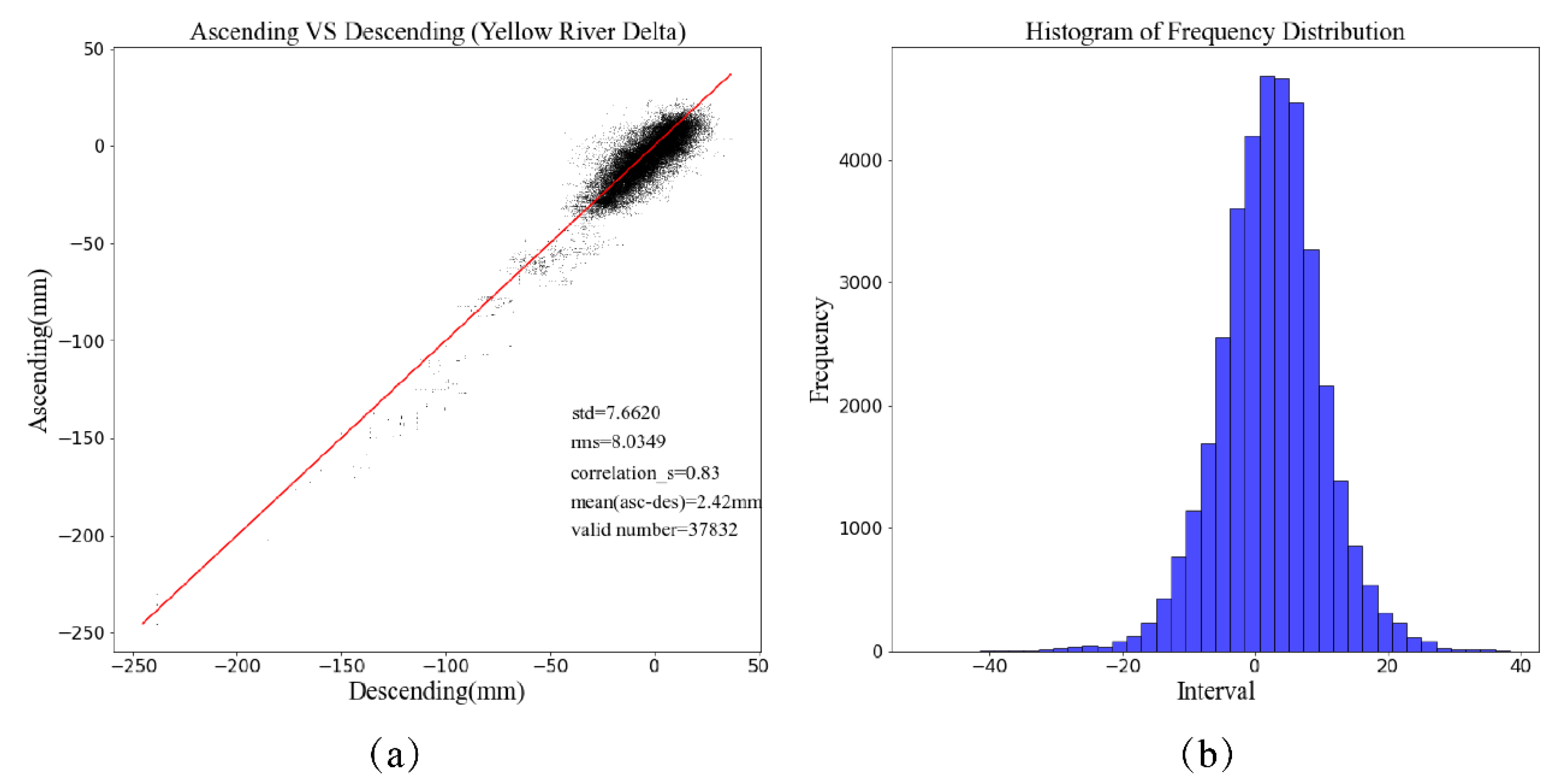
2.3.3. Accuracy Evaluation
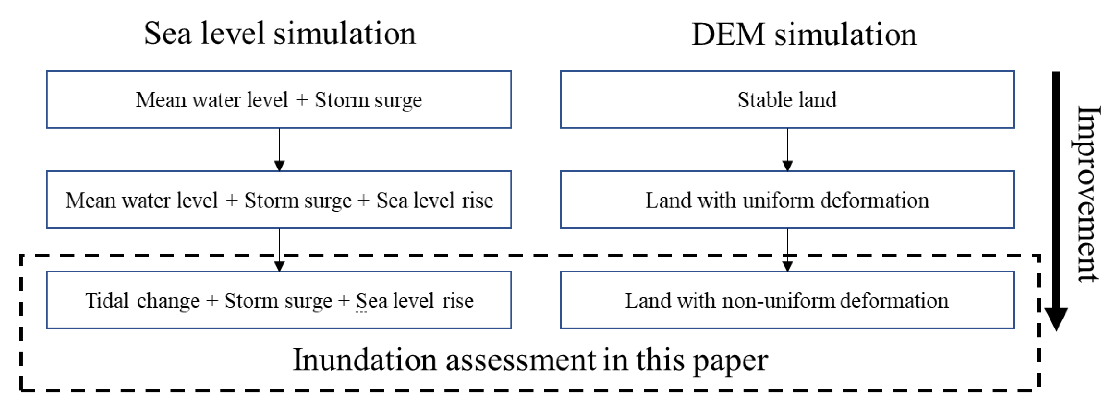
Both Figure 13 and Table 3 show the deformation rate comparison between the descending and ascending tracks. The correlation coefficient between the deformation rate of the entire Gudong Oilfield is 0.83 with a mean difference of 2.4 mm/year. The systematic negative bias is probably attributable to the selection of control points. From Figure 13b, and it can be seen that the errors fall into near normal distribution.
In the case of absence of long-term ground control points, we use cross validation method to verify the consistency and stability of the results. As far as the deformation rate map is concerned, we find that the law of deformation is basically positively correlated with human activities in the Gudong Oilfield. The large-scale subsidence in the upper part of Figure 12 over the coastal salt fields is very consistent with the extraction of underground brine. There also exists uplift in some areas over the Gudong Oilfield, which may be attributed to oil production method by injecting water into the underground oil layer to increase the pressure of the oil layer.

2.4. DEM Simulation

As the schematic diagram in Figure 14 shows, we performed clipping, interpolation and resampling on a raw deformation map. This process is critical to ensure that the deformation rate raster and the LiDAR DEM have the same geographic range and resolution. Then, we smoothed the obtained deformation rate raster with a threshold of 200 m to eliminate noise as far as possible and ensure that the deformation process was relatively smooth. By taking four sample points approximately evenly distributed over the dam as examples (Figure 15), the deformation rate is basically a linear trend. Thereafter, we simulated the future DEM through the operation of linear raster superposition, as illustrated in Figure 16.

2.5. Sea-Level Simulation

As an elongated strip-shaped artificial structure, the elevation of the Gudong coastal dam is largely below 5 m, and the elevation change is less than 2 m. Therefore, the simulation of sea-level must be sufficiently accurate and consistent with the reality. Here, we simulated a dynamic sea-level by considering the three components of tidal change, storm surge and sea-level rise.

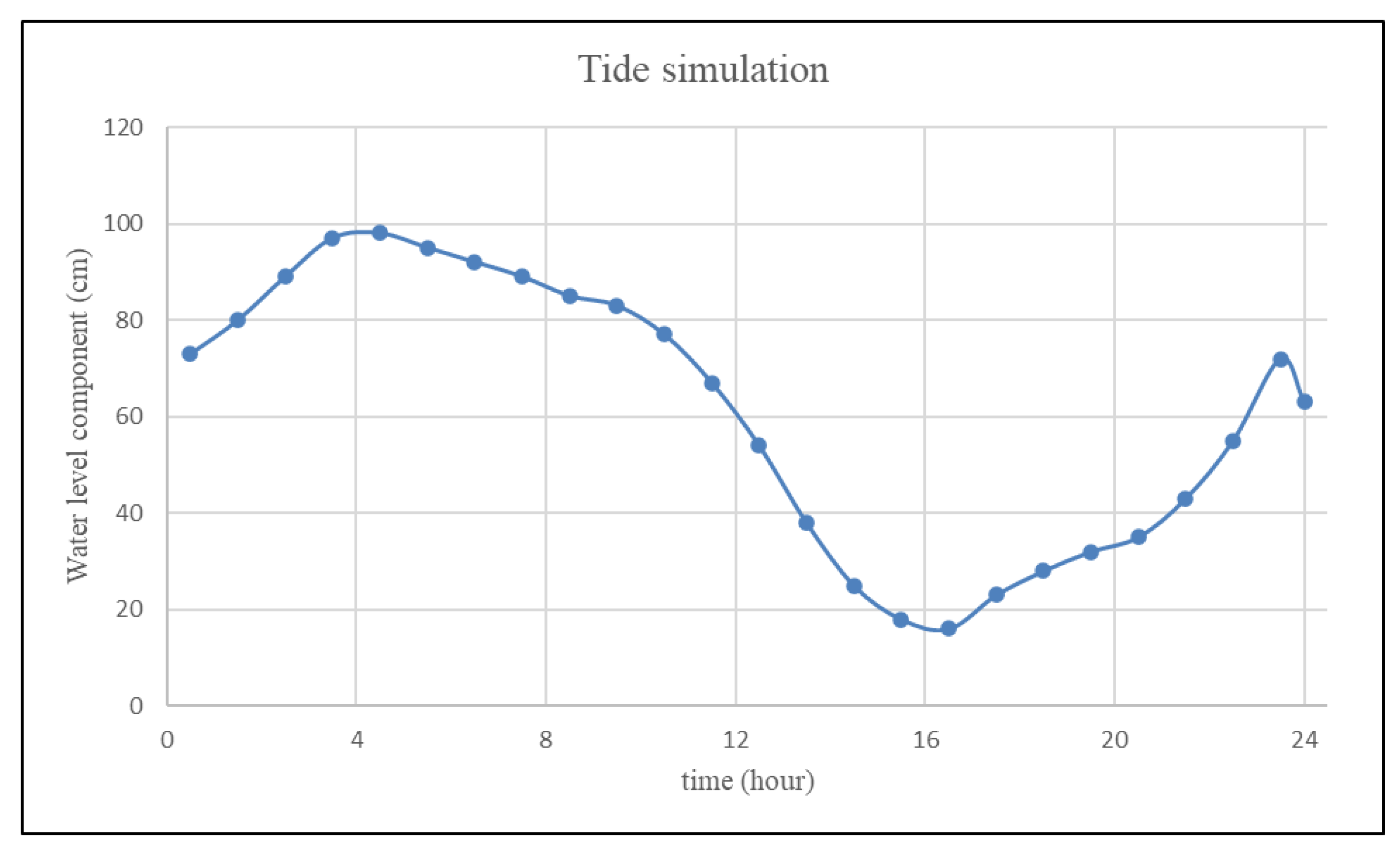
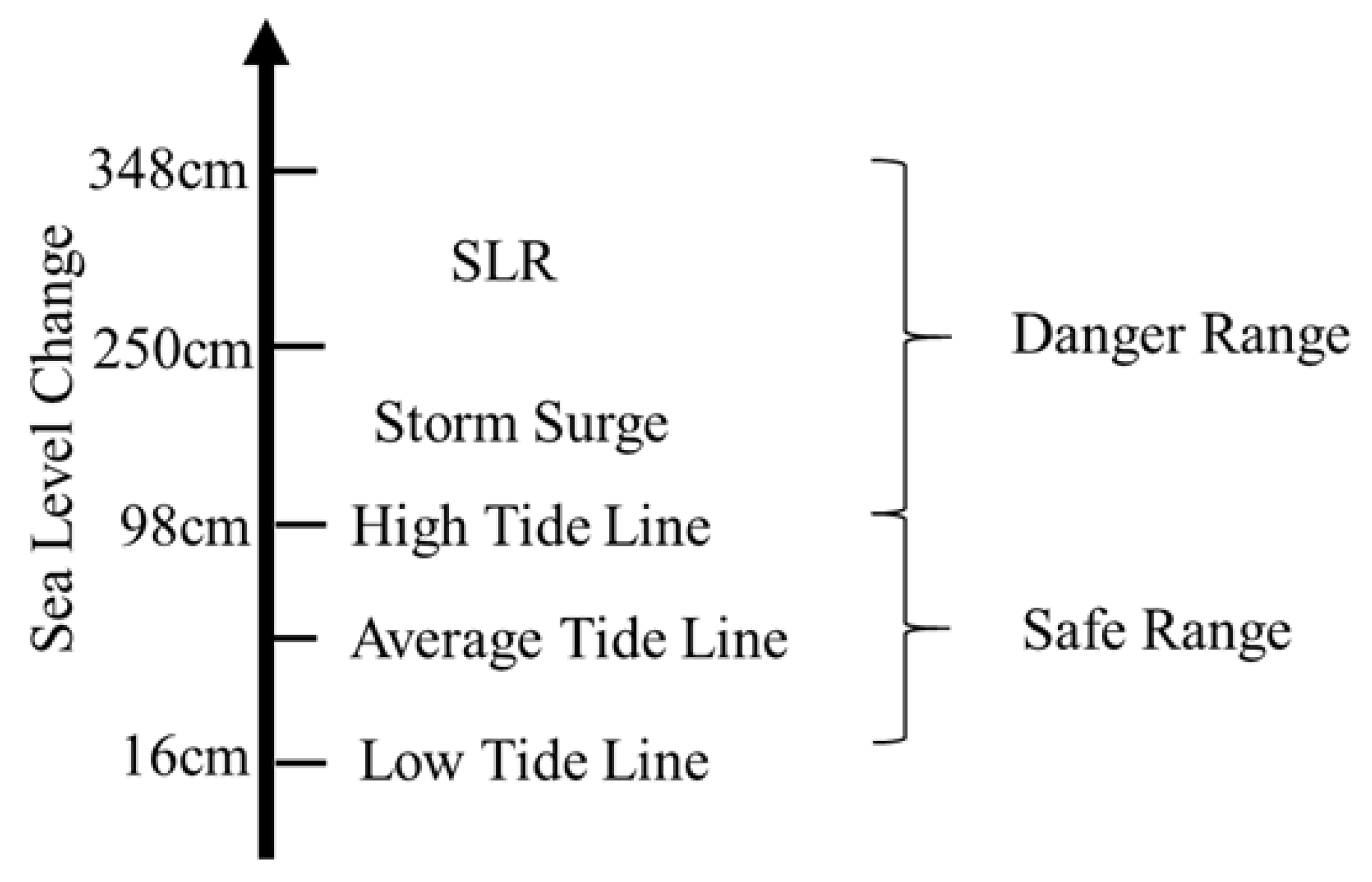
2.5.1. Tidal Change Simulation
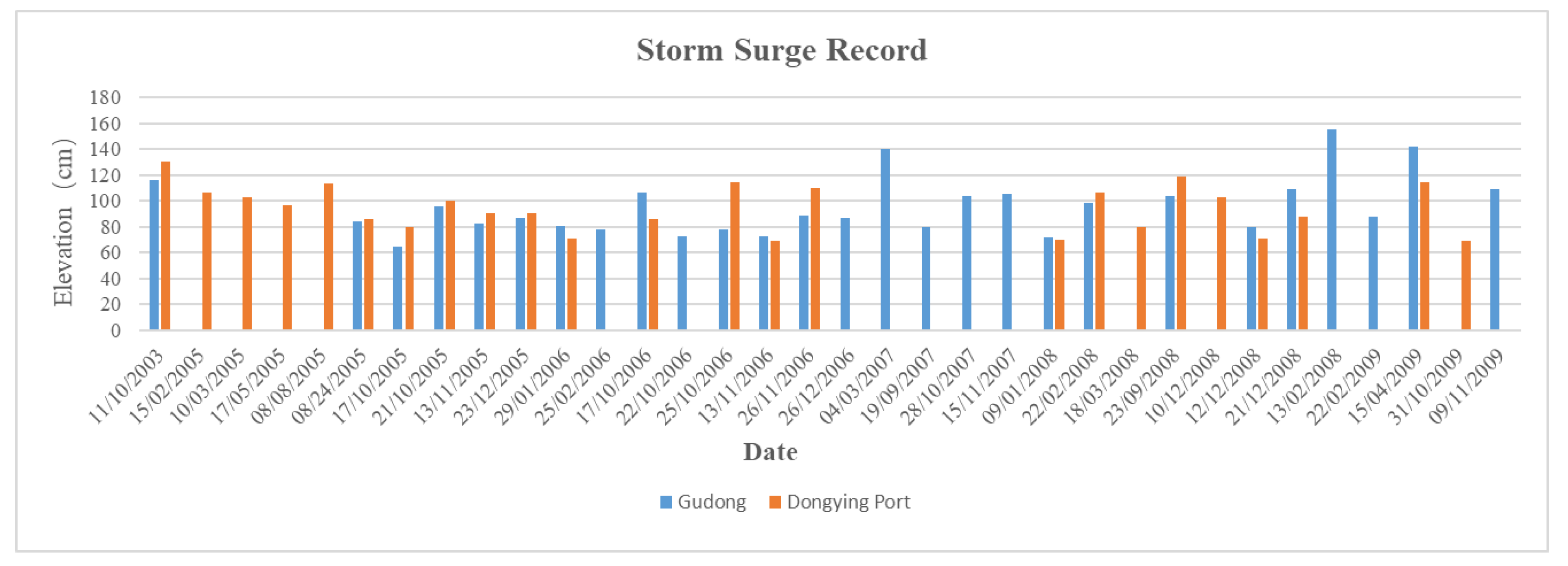
We refer to the prediction of the astronomical tide and interval of tide change released by the book “Coastal Warning Tidal Level Assessment in Shandong Province” [65]. Figure 17 presents the astronomical spring tide value range of 16–98 cm and the tide difference of 82 cm between spring tides and neaps. Due to high-standard structure adopted in the dam construction, Gudong coastal dam face major threats from extreme weather events. Among them, the greatest threat is the astronomical tide superimposed on the storm surge, whilst the smallest threat is the astronomical tide only. For the sake of simplicity, we adopt the height of spring tide (98 cm) as the starting point of water level simulation.
Moreover, according to the tidal data between 2018 and 2019 in the simulation of the waveform, we find that the tide of the Gudong area is a regular diurnal tide. Therefore, we simulated the tide change by referring to the above data. The simulated value of tidal change ranges from 16 to 98 cm. Based on this simulated tidal change, we superimposed the storm surge and sea-level rise.

2.5.2. Storm Surge

Storm surge is a kind of abnormal fluctuation of the sea caused by strong wind, sudden pressure changes caused by tropical cyclones (such as typhoons), temperate cyclones, or cold front strong weather systems. If the storm surge is overlapped with the astronomical tide, the sea-level will easily exceed the “warning line” and the seawater will break the embankment. Therefore, it is an important factor in the fluctuation of sea-level beyond the tide.
The storm surge records obtained from the China Meteorological Administration are shown in Figure 18 [65]. As indicated by the analysis of the data recorded by Gudong tidal gauge (the bigger pentagram in Figure 1b) and Dongying port tidal gauge, we set the storm surge interval from 0 to 150 cm.

2.5.3. Sea-Level Rise

Here, we refer to the predictions made by the IPCC in SLR simulation. With global warming exacerbated by human activities over the past 20 years, the melting of glaciers in Antarctica, Greenland and the Arctic region have been leading to continuous global sea-level rise. The present assessment report of projected future changes is primarily based on the predictions of a climate model using the RCPs [59]. The RCPs are a series of scenarios, including a time series of emissions and concentrations of greenhouse gases (GHGs), aerosols and chemically active gases, land use and land cover, which offer only one of the scenarios that could lead to varying degrees of global warming.
RCP 8.5 is the highest greenhouse gas emission scenario and leads to a continuous increase in the concentration of greenhouse gases in the atmosphere in the absence of policies to address climate change. By the end of this century, sea-levels will rise by 53 to 98 cm in the RCP 8.5. Here, we take the maximum value for the simulation of sea-level rise. Therefore, we simulate a sea-level rise of 10 cm in 2030, 33 cm in 2050 and 98 cm in 2100 [59].

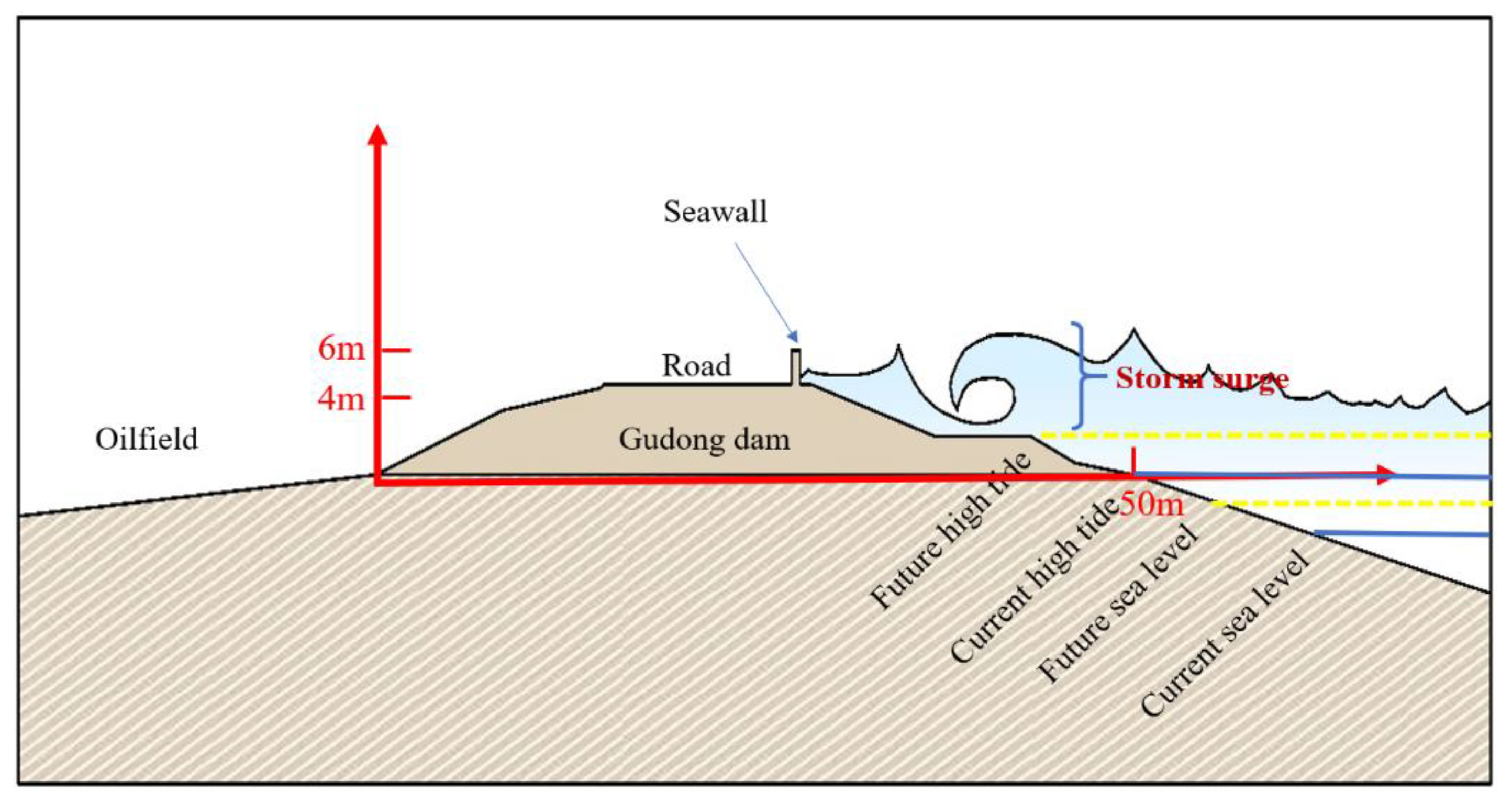
2.6. Bathtub Model for Inundation Assessment

The inundation assessment model we use here is a simple bathtub model [16,29,41,47]; that is, we superimpose the simulated future sea-level on the seaward side of the dam to obtain the submerged scene. In addition, as the dam is formed in the shape of a hump, when conducting inundation analysis, we should avoid the back of the dam that below the simulated water level is submerged too. Therefore, we have adopted a simple separation process to ensure that the submerged range is scientifically correct. The back of the dam should not be submerged before overtopping occurs. Figure 19 provides a schematic diagram of the bathtub model used, which is a four-way hydraulic connectivity rule, whereby a cell flows only if it is connected to a water body directly or via adjacent cells in cardinal directions [29]. The bathtub model is used to illustrate that the analysis of the seaward side and the back side is different when analyzing inundation. Although the elevation of the front and back of the dam is identical, only the front of the dam will be submerged when the seawater does not overflow the dam.

3. Results

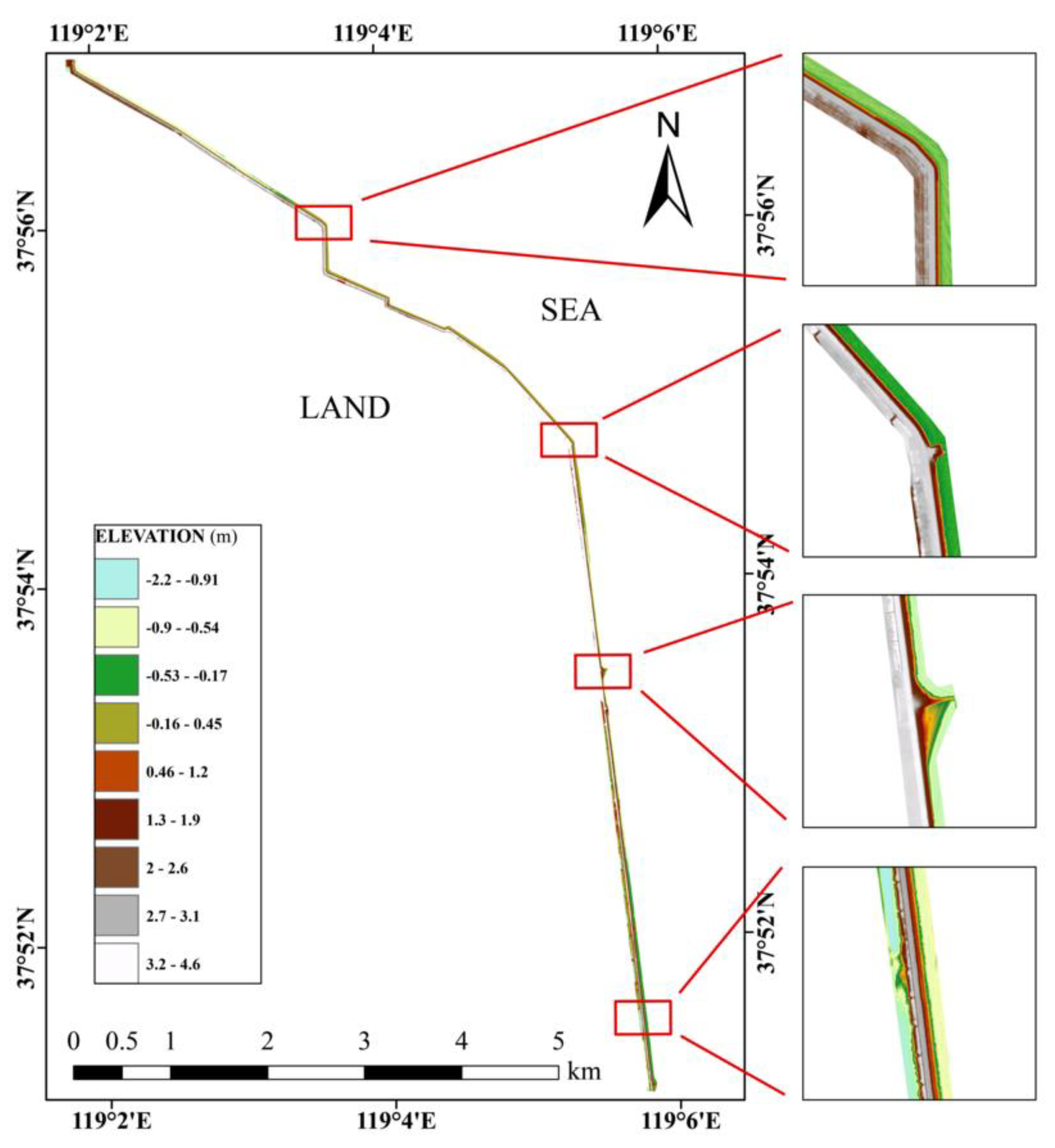
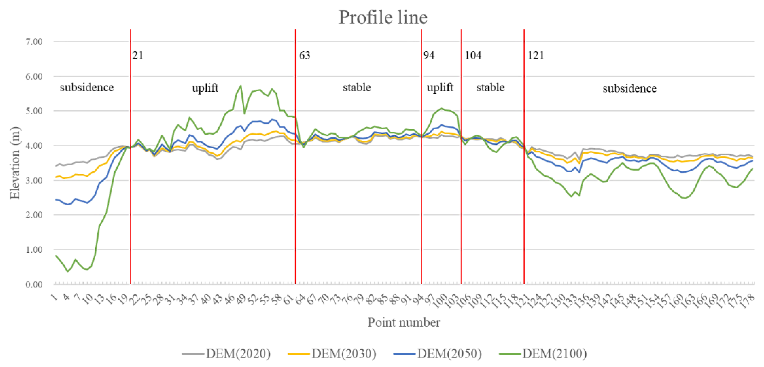
3.1. DEM Simulation Results

Figure 18 and Figure 19 show the simulated DEM in the form of a cross-section of four periods and a two-dimensional diagram for DEM for different periods. It can be seen that there is an obvious process of uplift between points 21–63 and 94–104 whilst a process of subsidence between points 1-20 and 121–178 is evident in Figure 20. As it is shown that deformation is below 50 cm, points 64–97 and 105–120 will be relatively stable after 80 years. In Figure 21, four columns present the DEM changes of the four representative fragments of Gudong Dam for the four different scenarios; that is, the years 2020, 2030, 2050 and 2100. The first two lines extracted from points 10 and 49 illustrate the main trend of rapid subsidence and uplift, while the last two lines extracted from points 68 and 163 show that the stability and slow subsidence trend is dominant.

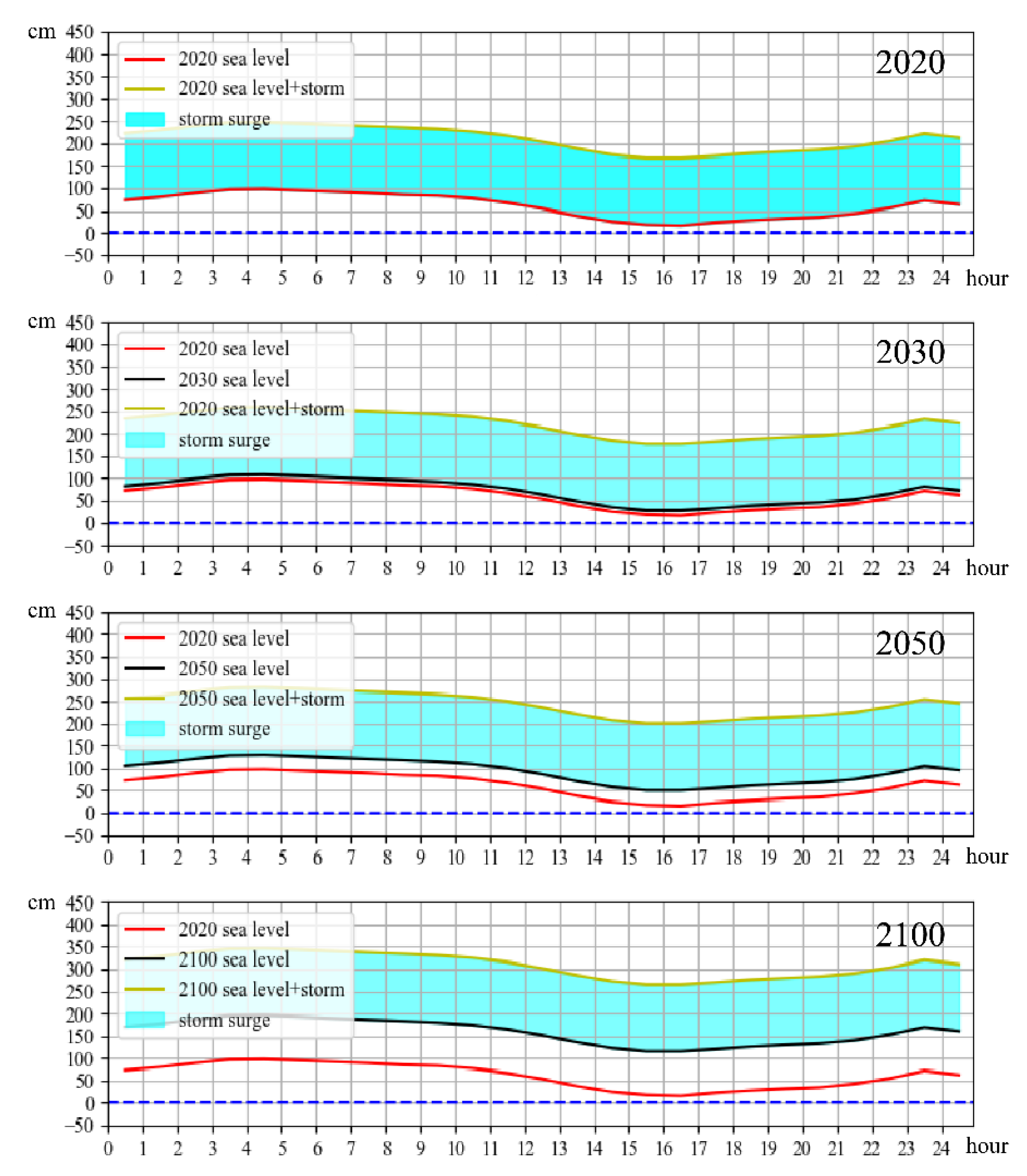
3.2. Sea-Level Simulation Results

Through the superposition of three components (tide change, SLR and storm surge), we simulated the sea-levels of 2020, 2030, 2050 and 2100 (Figure 22). It can be seen that, under the storm surge and sea-level rise, the rise of sea-level is very obvious. Considering an actual situation, when a storm surge occurs it is often accompanied by extremely high waves caused by strong winds. Therefore, the actual instantaneous sea-level and impact force that the dam will suffer will likely be more severe.
The method used for water level superposition is shown below. Here, we use a static linear method to superimpose the three components to obtain the water level values.
W L C = T C + S S + S L R
where WLC is water-level change, TC is tide change, SS is storm surge interval and SLR is the sea-level rise.
There are two important values in the sea-level simulation results; that is, the normal sea-level and the highest sea-level. The normal sea-level refers to the astronomical spring tide value that can easily be attained under normal weather conditions, whilst the highest sea-level indicates the highest sea-level height which can only be reached under extreme weather conditions. Table 4 details sea-level simulation results in regard to the four different scenarios that will be used for further analysis in the next section.

3.3. Inundation Assessment

As shown in Figure 23, the inundation assessment integrates the sea-level and DEM components to evaluate the flood control capacity of the coastal dam. Before considering this inundation assessment, two points should be noted: firstly, the elevation datum of the DEM and sea-level should be unified [28]; secondly, the maximum submergence is a transient state. At a leveling control point with known elevation near the tide gauge station (Figure 1b), we measured its WGS84 elevation, calculated the datum conversion difference and employed the same correction value to adjust the tide elevation. Finally, all elevations are unified under the WGS84 geodetic height system.

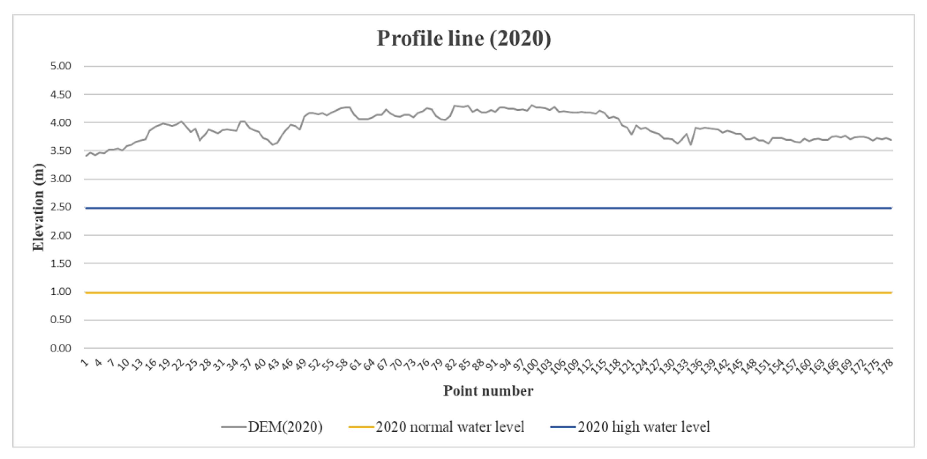
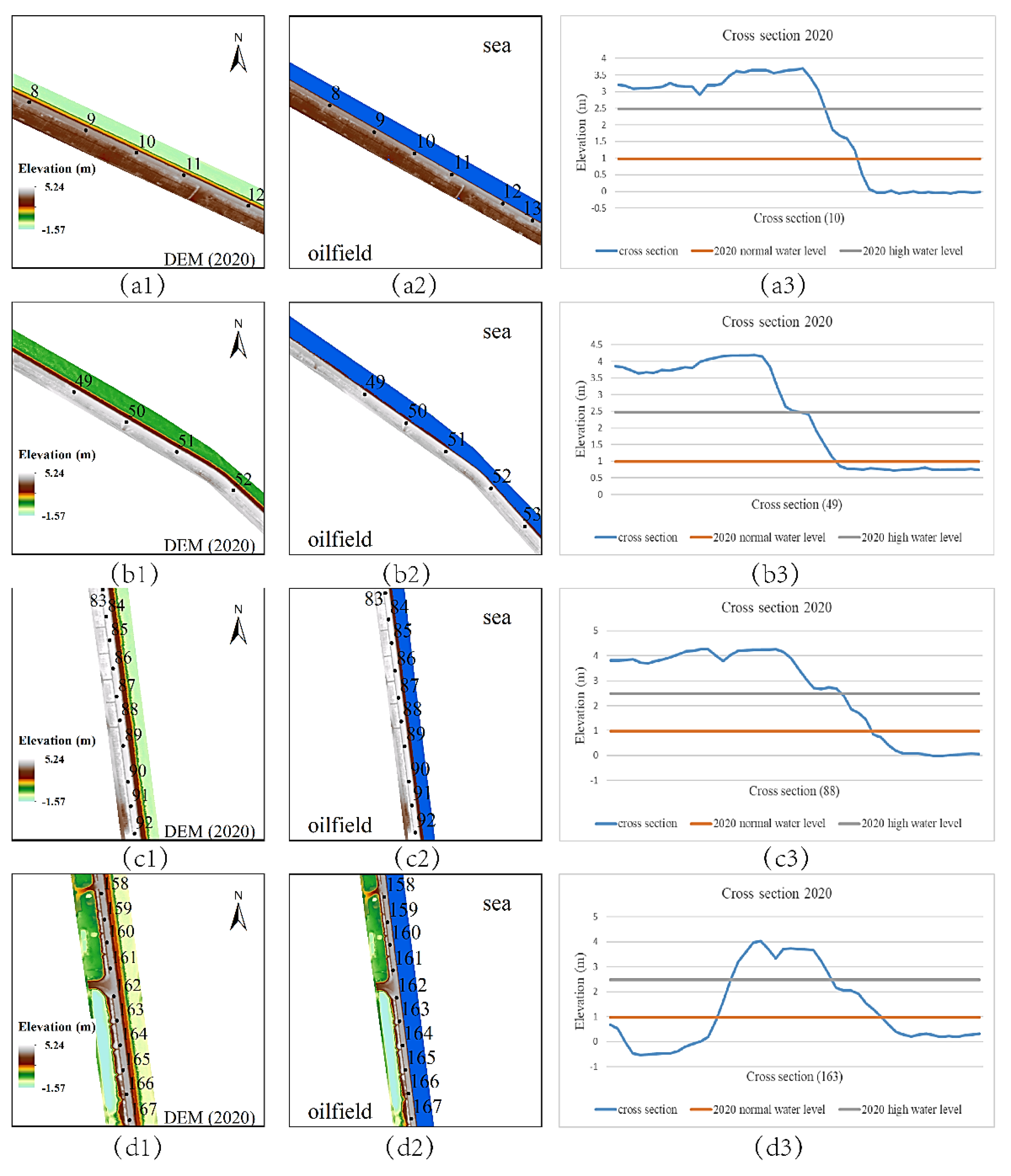
3.3.1. Scenario of 2020

Figure 24 is the profile of the DEM and water level in 2020, we can find that the sea-level will not be higher than the dam even under extreme weather conditions, which is consistent with the current actual situation. The highest point of the dam is 4.31 m and the lowest point is 3.41 m, both of which are higher than the high sea-level (2.48 m). However, in a situation of wind arriving from a particular direction, seawater can pour into the oilfield in the form of high waves. Taking Typhoon Lekima in August 2019 as an example, although the sea-level did not exceed the dam, waves of 3 m to 5 m high nevertheless led to a large amount of water inflow into the oilfield. Figure 25 shows the cross section of four different part of the dam and the overlap between the water level and the dam.

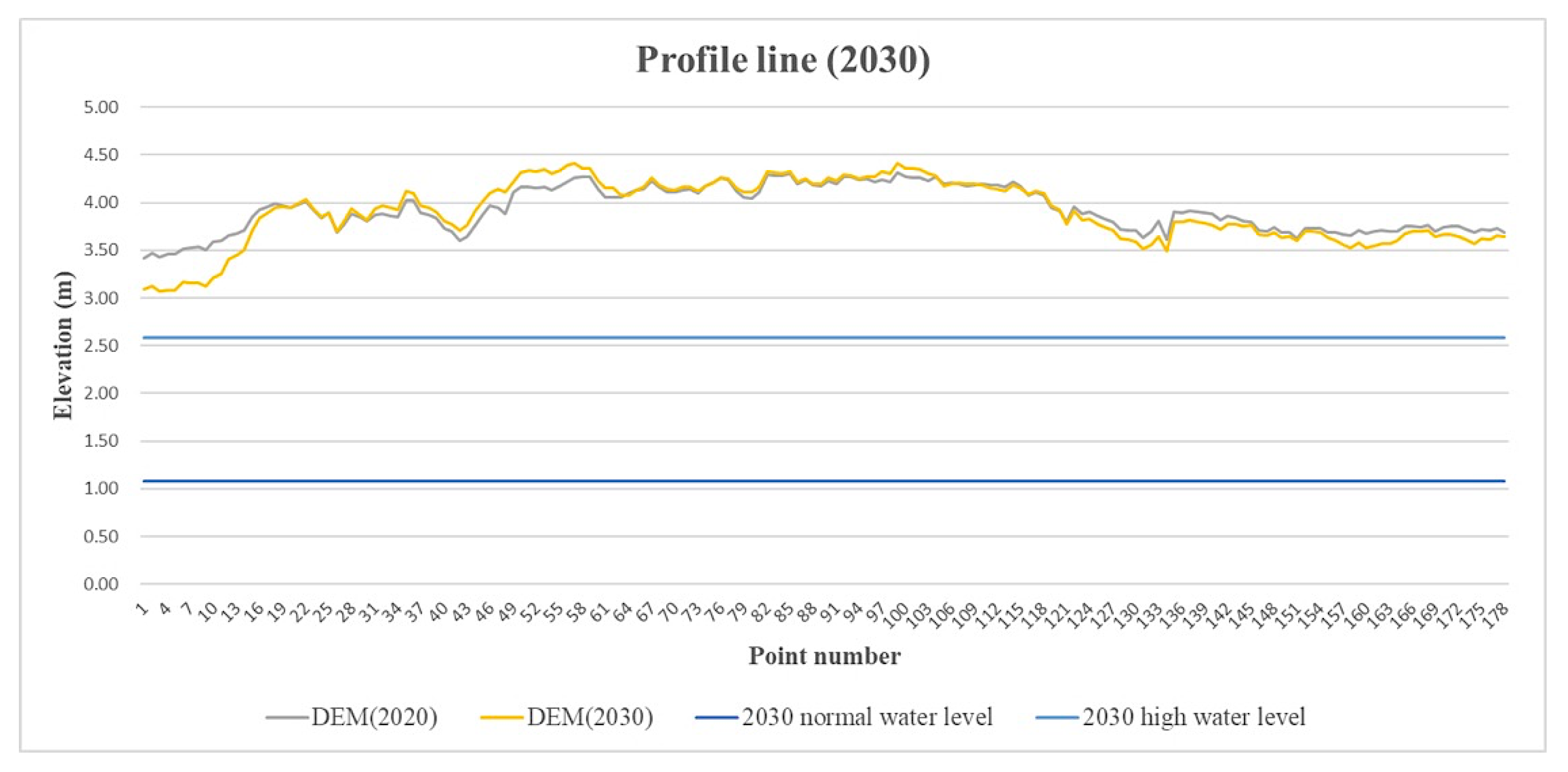
3.3.2. Scenario of 2030

As indicated in Figure 26 and Figure 27, the scenario of 2030 is similar to that of 2020 and there will be no invasion point. The highest point of the dam is 4.41 m and the lowest point is 3.07 m, both of which are higher than the high sea-level (2.58 m). However, the mean gap between the dam and sea-level has narrowed by 13 cm. In addition, the protective capacity of the northern end of the dam has declined, as indicated in Figure 26. Furthermore, deformation of the dam will also lead to the destruction of the structure of the dam itself.

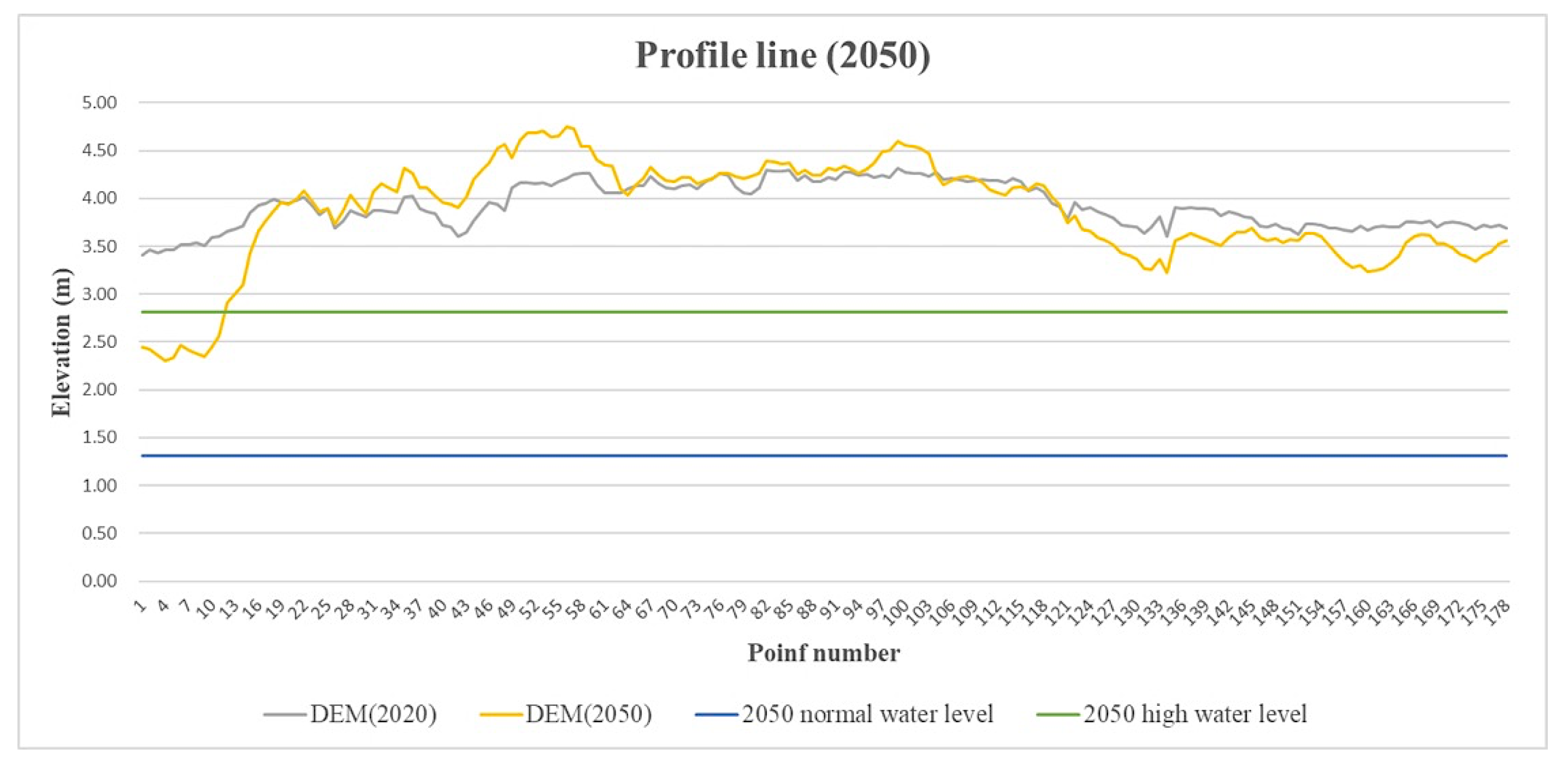
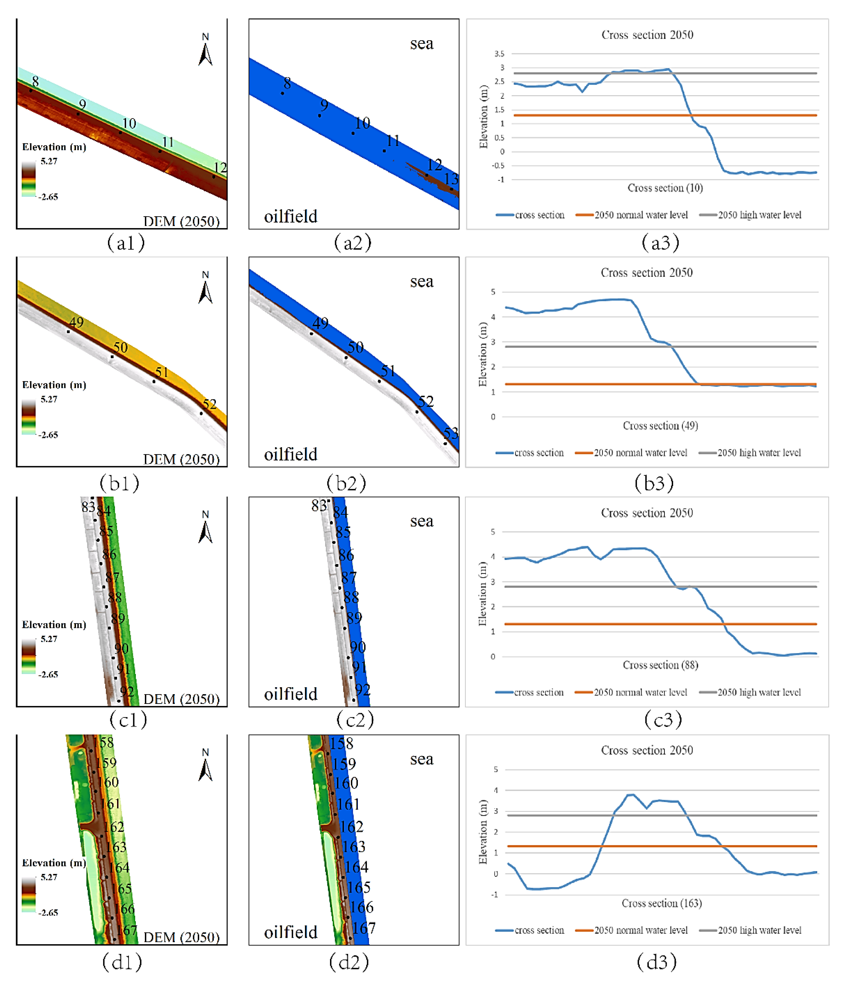
3.3.3. Scenario of 2050

After 30 years of continuous deformation, the dam can be seen to undergo significant changes in Figure 28 and Figure 29. The maximum subsidence is about 116 cm, while the maximum uplift is about 69 cm. With the normal sea-level (1.31 m), the highest point of the DEM 2050 is about 4.75 m, which is higher than the simulated sea-level, and the lowest point is about 2.30 m, which is higher than the simulated sea-level also.
With the highest sea-level (2.81 m), the highest point of the DEM 2050 is about 4.75 m, which is higher than the simulated sea-level. However, between points 1 and 11, the dam will be submerged easily. Additionally, between points 123 and 178, the difference between the sea-level and dam crest is less than 1m and the minimum value is 42 cm; therefore, the highest sea-level is close to the dam crest. Although the sea-level will not be higher than the dam under these extreme conditions, the protective ability of the coastal dam is very weak in consideration of the factor of wave.
Therefore, in combination with sea-level rise and vertical deformation of the dam, intrusion points will appear in around 2050, meaning that the protection capacity of the dam is already in jeopardy. Countermeasures should thus be taken prior to 2050, as, otherwise, seawater will easily pour into the oilfield.

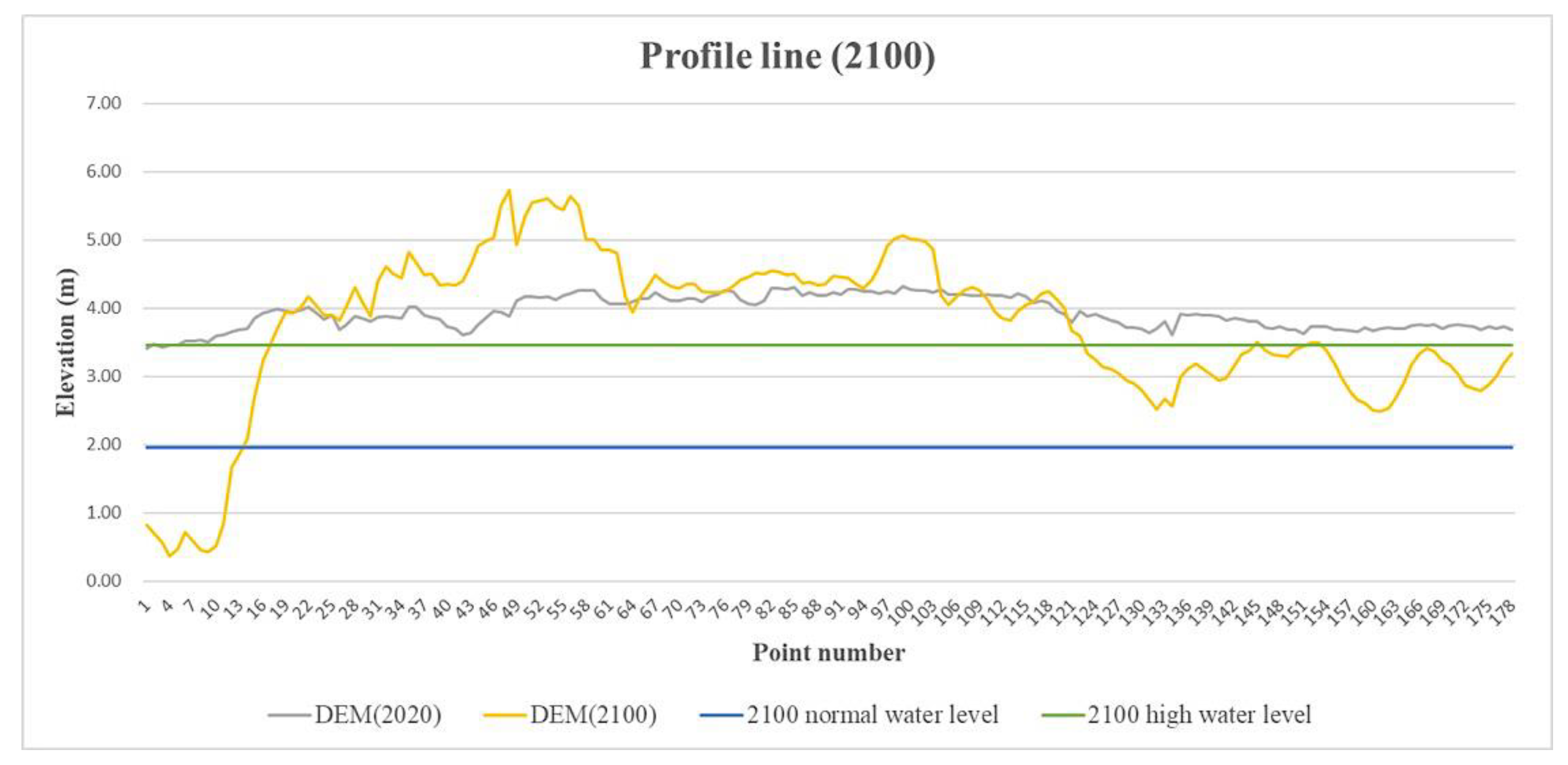
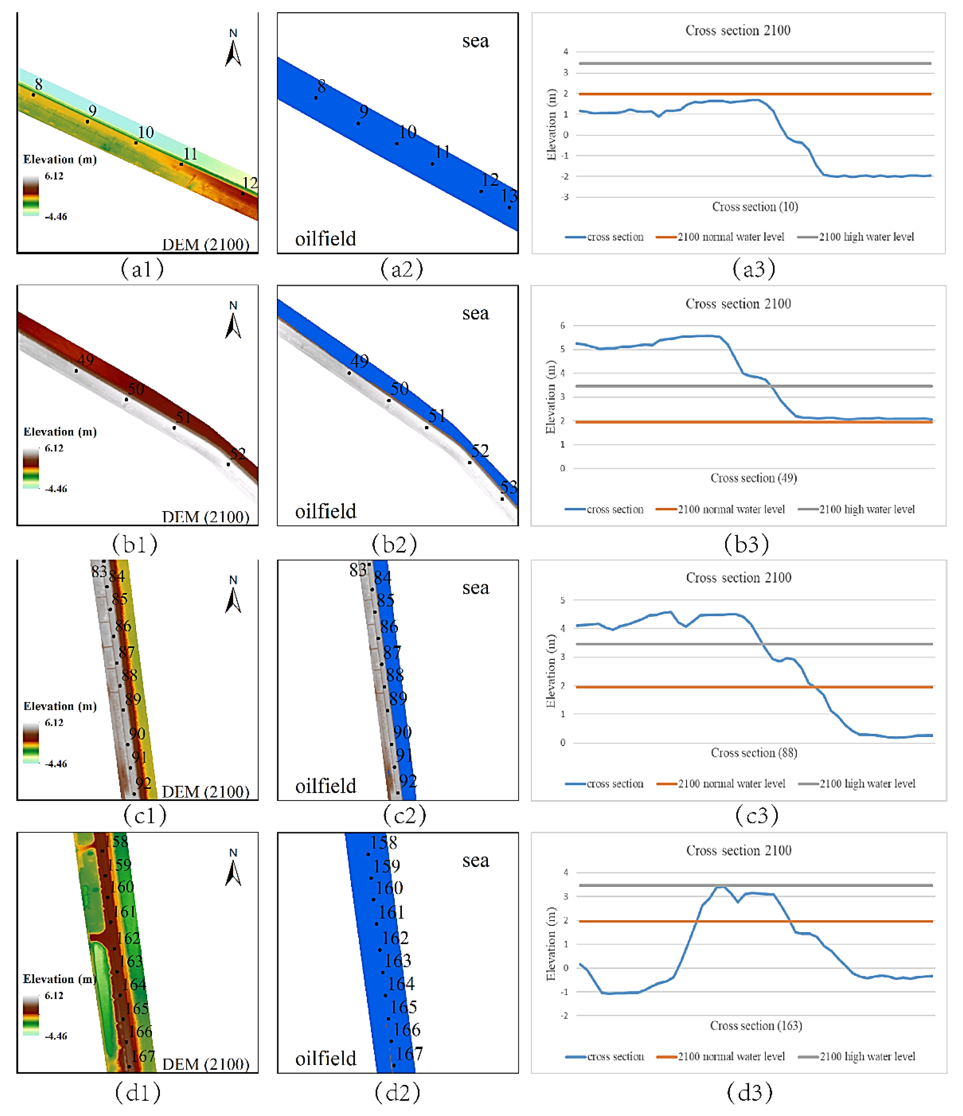
3.3.4. Scenario of 2100

Figure 30 and Figure 31 show that, by the end of this century, the situation will deteriorate further. With the normal sea-level (1.96 m), the highest point of the simulated DEM 2100 is about 3.76 m higher than the simulated sea-level. The protective ability of the dam between points 21 and 120 is still reliable, due to the overall rise of the ground but, from points 1 to 13, the dam will be easily submerged by seawater and an area of the dam at least 1.1km long will be submerged easily by seawater.
With the highest sea-level, the situation deteriorates further. The highest point of the simulated DEM 2100 is about 2.26 m above the simulated sea-level. The dam is completely submerged by seawater from points 1 to 17 and 123 to 178, and the unprotected section is up to about 4.41 km. At this time, the seawater and land will be connected on a large scale. Due to the low-lying topography of the Gudong area, the oilfield will be completely submerged by seawater. In addition, it can be seen from Figure 28 that, even without the consideration of the dam deformation in 2100, the protective capacity of the dam will also significantly decrease as a result of the sea-level rise alone.

4. Discussion

4.1. Selection of DEM for Inundation Assessment

There are many ways to obtain DEMs, such as InSAR, photogrammetry and LiDAR [43,44,66,67,68]. As an indispensable product in most areas of earth science, the DEM should be chosen carefully in terms of its resolution and accuracy. Products such as SRTM and AW3D30 in Table 5 [69], have been used widely in the civilian and military sectors [28,29,70] and indeed, offer significant advantages for large scale applications that do not require highly accurate quantitative analysis [31]. However, in the case of a long and narrow artificial low-lying coastal dam, such global DEMs cannot meet requirements in terms of precision, fineness, smoothness and other aspects.
In particular, the current DEM of the dam is the fundamental dataset for future DEM simulation and submergence assessment in different scenarios. Gesch [46] has proved that use of high-accuracy LiDAR-derived elevation data is an advantage for elevation-based assessments of coastal inundation events such as storm surges, abnormal high tides or extreme precipitation events. A DEM should have an accuracy of better than 25.5 cm (RMSE) when modeling of 1 m or less of sea-level rise, in order to avoid being within the bounds of the statistical uncertainty of the elevation data.
At present, the popularity of UAV, the miniaturization of LiDAR, and the combination of both, make the acquisition of DEM of a strip artificial structure more economical and effective. Moreover, a variety of processing on the point cloud, such as filtering and classification, are convenient. The fine DEM in this study was generated with a resolution of 20 cm through the filtered point cloud collected by the UAV LiDAR in August 2019 following Typhoon Lekima. Compared with previous articles related to submergence analysis [31,41,47], the DEM used in this article has greatly improved two important indicators, that is, the accuracy and spatial resolution, which is also a prerequisite for accurate analysis of fine artificial buildings and forest canopy. In general, UAV LiDAR is a necessary and effective way to achieve sub-meter accuracy DEM for coastal dam inundation assessment.

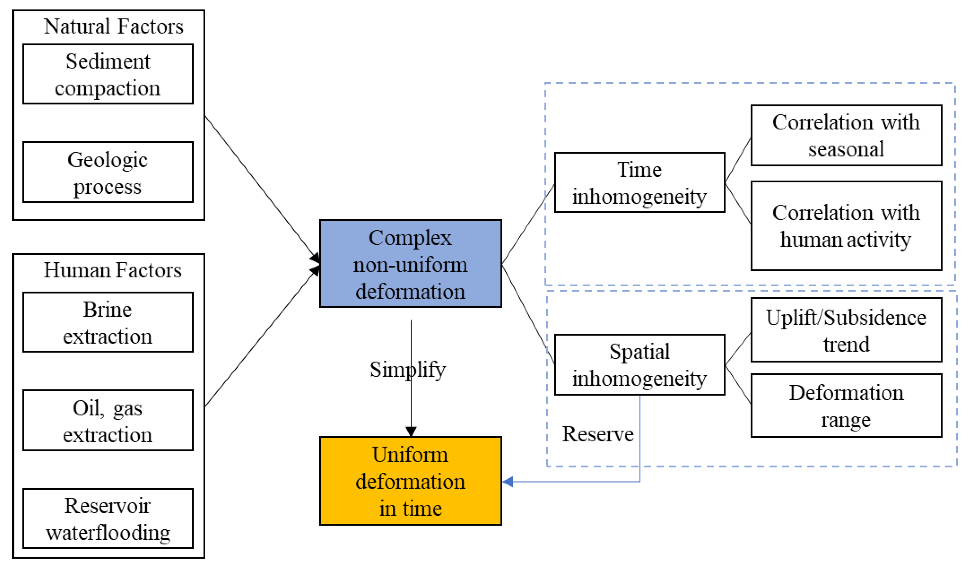
4.2. Coastal Dam Deformation and DEM Simulation

In order to obtain more accurate and dynamic results in inundation assessment, the DEM should update with the deformation. Some researchers used interpolation to simulate an uneven deformation rate grid with traditional monitoring data [32,34], or used an average value as deformation rate over the whole study area [33]. The SBAS InSAR technique has been developed over a period approaching 20 years can be used to measure and reveal the physical mechanism of land deformation [21]. Previous attempts to monitor the ongoing destabilization process of artificial dams using space-borne or ground-based (GB) InSAR outside the traditional leveling and GNSS measurement have largely focused on inland water reservoirs and hydraulic structures [51,71,72,73].
In this study, we revealed a complicated deformation pattern of the coastal dam consisting of both uplift and subsidence. As shown in the Figure 32, many natural and man-made factors contribute to the river delta deformation, which makes the stability of coastal dam uneven in time and space domain. Here some simplifications are made by preserving the spatial variation characteristics of deformation and ignoring the inhomogeneity in the time domain. In spatial dimension, the uplift is primarily caused by water injection during secondary oil recovery [74,75]. With the exploitation of oil and gas resources in the field of oil extraction, the pressure of the oil-bearing layer continues to be released, resulting in a drop in the pressure of the oil-bearing layer, which is then insufficient to push the oil out of the ground. In this case, the method of injecting water into the oil-bearing layer to increase the pressure is often used to ensure the continuation of oil extraction. Compared with the single inducement of ground uplift, there are more reasons for land collapse, such as the continuous mining of underground mineral resources, compaction caused by underground brine extraction and the compaction of sediments over the Yellow River Delta. Most of them are human related activities that are common in mining areas.
On the basis of understanding oil field activities and analyzing deformation laws, here, we use the method of superposing the current DEM and land deformation rate to simulate the future DEM. It should be noted that we simulated the future DEM under the assumption that the dam was in a stable deformation process [21], which simplified the process of simulation. Nonetheless, in fact the deformation process of the dam is more complex and is likely to be significantly affected by human factors. The subsidence of the dam will reduce its protective capacity, but it does not mean that the uplift will increase its protective capacity. In addition, there are both uplift and subsidence phenomena in part of the coastal dam body, in which the inconsistency of vertical direction will produce an extremely unfavorable shear stress on the structure and cause more serious damage to the dam. Given that the deformation direction is homogeneous, the uneven displacement velocity would also produce shear stress, albeit substantially lower.

4.3. Sea-Level Simulation

Several previous studies only used the concept of average sea-level, which greatly limits its practical application [17,26,36]. Figure 33 shows that the use of the mean water level reduces the estimated water level, which affects the results of the inundation analysis. In this study, we used three components to synthesize the simulated sea-level, including tidal changes, IPCC published sea level rise data and long-term storm surge records. Normal changes in water levels do not pose a threat to the coastal dam, but the real danger is at astronomical spring tides.
It should be noted that the tide gauge station would be susceptible to ground deformation without external position correction, such as GNSS [76]. Therefore, we used a simulated sea-level in order to avoid incorrectly estimating sea-level. Two values were used for inundation analysis—the normal sea-level and the highest sea-level [41]—one of which represents daily changes and the other extreme situations. Taking 2020 as a reference from which to verify the sea-level simulation results, the results are in line with the current actual situation. For example, taking Typhoon Lekima as an example, the sea-level was almost consistent with the actual situation.

4.4. Inundation Assessment Algorithm

The Gudong coastal dam was built with the highest engineering specifications over the Yellow River Delta area, with the dynamic environmental context taken into account. Most previous inundation studies focused on flooding range and depth over large-scale areas [35,56]. The coastal dam is the first and most vital security barrier at the sea-land interface. If the function of the dam were to be damaged, seawater would easily flow over the dam. It is easier to understand with the aid of a profile and a two-dimensional submerged range map intuitively displayed.
The data used in flood analysis involves a gradual transition from simple assumptions to complex simulations. In Figure 34, we sum up the experience of the predecessors, which is the premise to carry out the analysis of the vulnerability of coastal zone flooding. The bathtub model generally improves the shoreline water level on coastal DEM by selecting a land elevation higher than the current water level, and then selecting all areas at or below the elevation, which has been improved by accounting for hydrologic connectivity [46,77,78,79]. As an efficient hydrostatic model, we used a four-way hydraulic connectivity rule to analyze the inundation of the dam, where a cell flows only if it is connected to a water body directly or via adjacent cells in cardinal directions [29].
More complex hydrodynamic models have been studied, but are very time consuming and computationally intensive through an integrated tide-surge, wave and flooding modeling framework to accurately predict the flooding due to wave overtopping and represent cross-shore sediment transport processes explicitly with highly parameterized models [24,25]. Due to the potential for both inundation and dynamic response that exists for many coastal landscapes, a data-driven coastal response model could be more preferable as an alternative that considers both inundation and dynamic response using data sets describing elevation and vertical land movement at a range of sea level rise scenarios [80].

5. Conclusions

In this study, we present a systematic solution and a range of scenarios for coastal dam inundation assessment by combination of different space-based observations and simulation models. A high-resolution, high-accuracy DEM of Gudong Dam is generated with UAV LiDAR and a surface deformation rate map of the dam is created using the SBAS InSAR technique. Under the assumption that deformation rate is constant in the future, a simulated sea-level composed of three components was superimposed with the coastal DEM to analyze the flooding trend of the dam, using a bathtub model. This evaluation procedure is cost-effective and can be updated in time.
The results indicate that the protection capability of Gudong Dam is weakening year by year, as a result of dam deformation, sea-level rise and the increasing frequency of extreme weather events. Based on the analysis and predictions on the Gudong oilfield, the coastal dam protection ability is relatively safe and reliable in most cases, except for the heavy rainfall and large waves caused by extreme weather such as typhoon. Typhoon waves up to 3 to 5 m can break part of the retaining walls and bring a certain amount of seawater intrusion.
There will not be much change in 2030 compared to 2020. By 2050, it is highly likely that the dam will be flooded, and, in the case of high water levels, nearly 1 km of the dam’s northern length will be submerged. The rapid subsidence in this area is mainly due to the land subsidence caused by brine mining in the northern salt fields. By the end of the century, the coastal dam will have lost most of its protective capacity, and if high water levels occur, about 4.41 km of dam in the north and south will be completely submerged. On account of the relative stability and local uplift, the central part will not be submerged, but the protection ability is greatly reduced. Oil fields would be flooded by seawater, causing massive damage to the production facilities. Combined with these factors, the difficulty and cost of oil extraction will increase dramatically.
Therefore, we should reinforce the monitoring of the dam and revise the evaluation parameters in time in order to derive more accurate prediction results. In the future, the coastal dam will be strengthened or repaired only when damaged, which is more an afterthought than a preventive measure. This article can help to obtain the time node and specific locations requiring reinforcement and offers an alternative cost-effective approach for the protection of other artificial coastal infrastructures.

Author Contributions

Conceptualization, P.L. and Z.L.; methodology, P.L., G.W. and Z.L.; formal analysis and validation, P.L. and G.W.; investigation, G.W., P.L., D.D., L.Q., J.X., G.L. and H.W.; resources, P.L., Z.L., and G.L; writing—original draft preparation, G.W. and P.L.; writing—review & editing, P.L. and Z.L.; project administration, P.L. and Z.L.; data curation, G.W. and P.L.; visualization, G.W. and P.L.; supervision, P.L. and Z.L.; funding acquisition, P.L., Z.L., H.W. and G.L. All authors have read and agreed to the published version of the manuscript.

Funding

This work was jointly supported by the Natural Science Foundation of China (No. 41806108), National Key Research and Development Program of China (No. 2017YFE0133500; No. 2016YFA0600903), Open Research Fund of State Key Laboratory of Estuarine and Coastal Research (No. SKLEC-KF202002), Qingdao Indigenous Innovation Program (No. 16-5-1-25-jch) and Qingdao Postdoctoral Application Research Project. Z.H. Li was supported by the European Space Agency through the ESA-MOST DRAGON-5 Project (Ref.: 59339).

Acknowledgments

We are very grateful to those colleagues from the Ocean University of China for conducting GNSS and UAV LiDAR field measurements. All the Sentinel-1 data are freely available from the European Space Agency (ESA). Tide gauge data are provided by the Yellow River Oilfield Administration. SRTM data products distributed by NASA’s Land Processes Distributed Active Archive Center (LP DAAC) are freely available. Google Earth images are used to describe the location of the study area. In the process of sea-level simulation, we consulted the data from the “Warning Tide Level Verification of Shandong Coastal” and IPCC AR5 report. ENVI SARscape 5.5 was provided by ESRI. We also thank the three anonymous reviewers and Editors for the constructive comments and suggestions, which greatly help improve the quality of this manuscript.

Conflicts of Interest

The authors declare no conflict of interest.

References

  1. Zhang, B.; Wang, R.; Deng, Y.; Ma, P.; Lin, H.; Wang, J. Mapping the Yellow River Delta land subsidence with multitemporal SAR interferometry by exploiting both persistent and distributed scatterers. Isprs J. Photogramm. Remote Sens. 2019, 148, 157–173. [Google Scholar] [CrossRef]
  2. Wu, X.; Bi, N.; Xu, J.; Nittrouer, J.A.; Yang, Z.; Saito, Y.; Wang, H. Stepwise morphological evolution of the active Yellow River (Huanghe) delta lobe (1976–2013): Dominant roles of riverine discharge and sediment grain size. Geomorphology 2017, 292, 115–127. [Google Scholar] [CrossRef]
  3. Narayan, S.; Beck, M.W.; Wilson, P.; Thomas, C.J.; Guerrero, A.; Shepard, C.C.; Reguero, B.G.; Franco, G.; Ingram, J.C.; Trespalacios, D. The Value of Coastal Wetlands for Flood Damage Reduction in the Northeastern USA. Sci. Rep. 2017, 7, 9463. [Google Scholar] [CrossRef]
  4. Grilli, A.; Spaulding, M.L.; Oakley, B.A.; Damon, C. Mapping the coastal risk for the next century, including sea level rise and changes in the coastline: Application to Charlestown RI, USA. Nat. Hazards 2017, 88, 389–414. [Google Scholar] [CrossRef]
  5. Li, Z.; Fielding, E.J.; Cross, P. Integration of InSAR Time-Series Analysis and Water-Vapor Correction for Mapping Postseismic Motion After the 2003 Bam (Iran) Earthquake. IEEE Trans. Geosci. Remote Sens. 2009, 47, 3220–3230. [Google Scholar] [CrossRef] [Green Version]
  6. Zhang, J.-Z.; Huang, H.-J.; Bi, H.-B. Land subsidence in the modern Yellow River Delta based on InSAR time series analysis. Nat. Hazards 2014, 75, 2385–2397. [Google Scholar] [CrossRef]
  7. Liu, P.; Li, Q.; Li, Z.; Hoey, T.; Liu, Y.; Wang, C. Land Subsidence over Oilfields in the Yellow River Delta. Remote Sens. 2015, 7, 1540–1564. [Google Scholar] [CrossRef] [Green Version]
  8. Liu, Y.; Huang, H.; Dong, J. Large-area land subsidence monitoring and mechanism research using the small baseline subset interferometric synthetic aperture radar technique over the Yellow River Delta, China. J. Appl. Remote Sens. 2015, 9. [Google Scholar] [CrossRef]
  9. Syvitski, J.P.M.; Kettner, A.J.; Overeem, I.; Hutton, E.W.H.; Hannon, M.T.; Brakenridge, G.R.; Day, J.; Vörösmarty, C.; Saito, Y.; Giosan, L.; et al. Sinking deltas due to human activities. Nat. Geosci. 2009, 2, 681. [Google Scholar] [CrossRef]
  10. Liu, Y.; Huang, H.; Liu, Y.; Bi, H. Linking land subsidence over the Yellow River delta, China, to hydrocarbon exploitation using multi-temporal InSAR. Nat. Hazards 2016, 84, 271–291. [Google Scholar] [CrossRef]
  11. Frihy, O.; Sayed, E.; Deabes, E.; Gamai, I. Shelf Sediments of Alexandria Region, Egypt: Explorations and Evaluation of Offshore Sand Sources for Beach Nourishment and Transport Dispersion. Mar. Georesour. Geotechnol. 2010, 28, 250–274. [Google Scholar] [CrossRef]
  12. Teatini, P.; Tosi, L.; Strozzi, T. Quantitative evidence that compaction of Holocene sediments drives the present land subsidence of the Po Delta, Italy. J. Geophys. Res. Solid Earth 2011, 116. [Google Scholar] [CrossRef]
  13. Teatini, P.; Tosi, L.; Strozzi, T.; Carbognin, L.; Cecconi, G.; Rosselli, R.; Libardo, S. Resolving land subsidence within the Venice Lagoon by persistent scatterer SAR interferometry. Phys. Chem. Earth Parts A/B/C 2012, 40–41, 72–79. [Google Scholar] [CrossRef]
  14. Higgins, S. Review: Advances in delta-subsidence research using satellite methods. Hydrogeol. J. 2015, 24. [Google Scholar] [CrossRef]
  15. Matano, F.; Sacchi, M.; Vigliotti, M.; Ruberti, D. Subsidence Trends of Volturno River Coastal Plain (Northern Campania, Southern Italy) Inferred by SAR Interferometry Data. Geosciences 2018, 8, 8. [Google Scholar] [CrossRef] [Green Version]
  16. Gebremichael, E.; Sultan, M.; Becker, R.; El Bastawesy, M.; Cherif, O.; Emil, M. Assessing Land Deformation and Sea Encroachment in the Nile Delta: A Radar Interferometric and Inundation Modeling Approach. J. Geophys. Res. Solid Earth 2018, 123, 3208–3224. [Google Scholar] [CrossRef]
  17. Dismukes, D.E.; Narra, S. Sea-Level Rise and Coastal Inundation: A Case Study of the Gulf Coast Energy Infrastructure. Nat. Resour. 2018, 9, 150–174. [Google Scholar] [CrossRef] [Green Version]
  18. Hinkel, J.; Lincke, D.; Vafeidis, A.T.; Perrette, M.; Nicholls, R.J.; Tol, R.S.; Marzeion, B.; Fettweis, X.; Ionescu, C.; Levermann, A. Coastal flood damage and adaptation costs under 21st century sea-level rise. Proc. Natl. Acad. Sci. USA 2014, 111, 3292–3297. [Google Scholar] [CrossRef] [Green Version]
  19. Kantamaneni, K. Coastal infrastructure vulnerability: An integrated assessment model. Nat. Hazards 2016, 84, 139–154. [Google Scholar] [CrossRef] [Green Version]
  20. Andreucci, R.; Aktas, C.B. Vulnerability of coastal Connecticut to sea level rise: Land inundation and impacts to residential property. Civ. Eng. Environ. Syst. 2017, 34, 89–103. [Google Scholar] [CrossRef]
  21. Ciro Aucelli, P.P.; Di Paola, G.; Incontri, P.; Rizzo, A.; Vilardo, G.; Benassai, G.; Buonocore, B.; Pappone, G. Coastal inundation risk assessment due to subsidence and sea level rise in a Mediterranean alluvial plain (Volturno coastal plain–southern Italy). Estuar. Coast. Shelf Sci. 2017, 198, 597–609. [Google Scholar] [CrossRef]
  22. Hind, A.; Aïcha, B.; Soufiane, H.; Mounir, H.; Tarik, B.; Boko, M.; Bouchaib, M. Evaluating the impacts of sea-level rise on the Moroccan coast: Quantifying coastal erosion and inundation in a Atlantic alluvial plain (Kenitra coastal). Episodes 2017, 40, 269–278. [Google Scholar] [CrossRef] [Green Version]
  23. Edmonds, D.A.; Caldwell, R.L.; Brondizio, E.S.; Siani, S.M.O. Coastal flooding will disproportionately impact people on river deltas. Nat. Commun. 2020, 11, 4741. [Google Scholar] [CrossRef] [PubMed]
  24. Barnard, P.L.; Erikson, L.H.; Foxgrover, A.C.; Hart, J.A.F.; Limber, P.; O’Neill, A.C.; van Ormondt, M.; Vitousek, S.; Wood, N.; Hayden, M.K.; et al. Dynamic flood modeling essential to assess the coastal impacts of climate change. Sci. Rep. 2019, 9, 4309. [Google Scholar] [CrossRef] [PubMed] [Green Version]
  25. Xie, D.; Zou, Q.-P.; Mignone, A.; MacRae, J.D. Coastal flooding from wave overtopping and sea level rise adaptation in the northeastern USA. Coast. Eng. 2019, 150, 39–58. [Google Scholar] [CrossRef]
  26. Gracia, V.; Sierra, J.P.; Gómez, M.; Pedrol, M.; Sampé, S.; García-León, M.; Gironella, X. Assessing the impact of sea level rise on port operability using LiDAR-derived digital elevation models. Remote Sens. Environ. 2019, 232. [Google Scholar] [CrossRef]
  27. Mohd, F.; Maulud, K.; A Karim, O.; Begum, R.; Awang, N.; Hamid, M.; Rahim, N.; Razak, A. Assessment of coastal inundation of low lying areas due to sea level rise. IOP Conf. Ser. Earth Environ. Sci. 2018, 169, 012046. [Google Scholar] [CrossRef]
  28. Refaat, M.M.; Eldeberky, Y. Assessment of Coastal Inundation due to Sea-Level Rise along the Mediterranean Coast of Egypt. Mar. Geod. 2016, 39, 290–304. [Google Scholar] [CrossRef]
  29. Yunus, A.; Avtar, R.; Kraines, S.; Yamamuro, M.; Lindberg, F.; Grimmond, C. Uncertainties in Tidally Adjusted Estimates of Sea Level Rise Flooding (Bathtub Model) for the Greater London. Remote Sens. 2016, 8, 366. [Google Scholar] [CrossRef] [Green Version]
  30. Yin, J.; Yu, D.; Lin, N.; Wilby, R.L. Evaluating the cascading impacts of sea level rise and coastal flooding on emergency response spatial accessibility in Lower Manhattan, New York City. J. Hydrol. 2017, 555, 648–658. [Google Scholar] [CrossRef] [Green Version]
  31. Bove, G.; Becker, A.; Sweeney, B.; Vousdoukas, M.; Kulp, S. A method for regional estimation of climate change exposure of coastal infrastructure: Case of USVI and the influence of digital elevation models on assessments. Sci. Total Environ. 2020, 710, 136162. [Google Scholar] [CrossRef]
  32. Yin, J.; Yu, D.; Wilby, R. Modelling the impact of land subsidence on urban pluvial flooding: A case study of downtown Shanghai, China. Sci. Total Environ. 2016, 544, 744–753. [Google Scholar] [CrossRef] [Green Version]
  33. Marfai, M.A.; King, L. Potential vulnerability implications of coastal inundation due to sea level rise for the coastal zone of Semarang city, Indonesia. Environ. Geol. 2007, 54, 1235–1245. [Google Scholar] [CrossRef]
  34. Wang, J.; Gao, W.; Xu, S.; Yu, L. Evaluation of the combined risk of sea level rise, land subsidence, and storm surges on the coastal areas of Shanghai, China. Clim. Chang. 2012, 115, 537–558. [Google Scholar] [CrossRef]
  35. Antonioli, F.; Anzidei, M.; Amorosi, A.; Lo Presti, V.; Mastronuzzi, G.; Deiana, G.; De Falco, G.; Fontana, A.; Fontolan, G.; Lisco, S.; et al. Sea-level rise and potential drowning of the Italian coastal plains: Flooding risk scenarios for 2100. Q. Sci. Rev. 2017, 158, 29–43. [Google Scholar] [CrossRef] [Green Version]
  36. Shirzaei, M.; Burgmann, R. Global climate change and local land subsidence exacerbate inundation risk to the San Francisco Bay Area. Sci. Adv. 2018, 4, eaap9234. [Google Scholar] [CrossRef] [Green Version]
  37. Wang, H.-W.; Lin, C.-W.; Yang, C.-Y.; Ding, C.-F.; Hwung, H.-H.; Hsiao, S.-C. Assessment of Land Subsidence and Climate Change Impacts on Inundation Hazard in Southwestern Taiwan. Irrig. Drain 2018, 67, 26–37. [Google Scholar] [CrossRef]
  38. Chen, C.-N.; Tfwala, S. Impacts of Climate Change and Land Subsidence on Inundation Risk. Water 2018, 10, 157. [Google Scholar] [CrossRef] [Green Version]
  39. Kulp, S.; Strauss, B.H. Global DEM Errors Underpredict Coastal Vulnerability to Sea Level Rise and Flooding. Front. Earth Sci. 2016, 4. [Google Scholar] [CrossRef]
  40. Loftis, J.D.; Wang, H.V.; DeYoung, R.J.; Ball, W.B. Using Lidar Elevation Data to Develop a Topobathymetric Digital Elevation Model for Sub-Grid Inundation Modeling at Langley Research Center. J. Coast. Res. 2016, 76, 134–148. [Google Scholar] [CrossRef] [Green Version]
  41. Gesch, D.; Palaseanu-Lovejoy, M.; Danielson, J.; Fletcher, C.; Kottermair, M.; Barbee, M.; Jalandoni, A. Inundation Exposure Assessment for Majuro Atoll, Republic of the Marshall Islands Using A High-Accuracy Digital Elevation Model. Remote Sens. 2020, 12, 154. [Google Scholar] [CrossRef] [Green Version]
  42. Gesch, D.B. Analysis of Lidar Elevation Data for Improved Identification and Delineation of Lands Vulnerable to Sea-Level Rise. J. Coast. Res. 2009, 53, 49–58. [Google Scholar] [CrossRef]
  43. Chang, H.-C.; Ge, L.; Rizos, C.; Milne, T. Validation of DEMs derived from radar interferometry, airborne laser scanning and photogrammetry by using GPS-RTK. In Proceedings of the 2004 IEEE International Geoscience and Remote Sensing Symposium, Anchorage, AK, USA, 20–24 September 2004; Volume 5, pp. 2815–2818. [Google Scholar]
  44. Pipaud, I.; Loibl, D.; Lehmkuhl, F. Evaluation of TanDEM-X elevation data for geomorphological mapping and interpretation in high mountain environments—A case study from SE Tibet, China. Geomorphology 2015, 246, 232–254. [Google Scholar] [CrossRef]
  45. Sefercik, U.G.; Yastikli, N.; Dana, I. DEM Extraction in Urban Areas Using High-Resolution TerraSAR-X Imagery. J. Indian Soc. Remote Sens. 2013, 42, 279–290. [Google Scholar] [CrossRef]
  46. Gesch, D.B. Consideration of Vertical Uncertainty in Elevation-Based Sea-Level Rise Assessments: Mobile Bay, Alabama Case Study. J. Coast. Res. 2013, 197–210. [Google Scholar] [CrossRef]
  47. Gesch, D.B. Best Practices for Elevation-Based Assessments of Sea-Level Rise and Coastal Flooding Exposure. Front. Earth Sci. 2018, 6. [Google Scholar] [CrossRef] [Green Version]
  48. Aly, M.H.; Klein, A.G.; Zebker, H.A.; Giardino, J.R. Land subsidence in the Nile Delta of Egypt observed by persistent scatterer interferometry. Remote Sens. Lett. 2012, 3, 621–630. [Google Scholar] [CrossRef]
  49. Liu, P. InSAR Observations and Modeling of Earth Surface Displacements in the Yellow River Delta. Ph.D. Dissertation, University of Glasgow, Glasgow, UK, 2012. [Google Scholar]
  50. Zhang, Y.; Wu, H.a.; Kang, Y.; Zhu, C. Ground Subsidence in the Beijing-Tianjin-Hebei Region from 1992 to 2014 Revealed by Multiple SAR Stacks. Remote Sens. 2016, 8, 675. [Google Scholar] [CrossRef] [Green Version]
  51. Al-Husseinawi, Y.; Li, Z.; Clarke, P.; Edwards, S. Evaluation of the Stability of the Darbandikhan Dam after the 12 November 2017 Mw 7.3 Sarpol-e Zahab (Iran–Iraq Border) Earthquake. Remote Sens. 2018, 10, 1426. [Google Scholar] [CrossRef] [Green Version]
  52. Oliver-Cabrera, T.; Wdowinski, S. InSAR-Based Mapping of Tidal Inundation Extent and Amplitude in Louisiana Coastal Wetlands. Remote Sens. 2016, 8, 393. [Google Scholar] [CrossRef] [Green Version]
  53. Buchanan, M.K.; Oppenheimer, M.; Kopp, R.E. Amplification of flood frequencies with local sea level rise and emerging flood regimes. Environ. Res. Lett. 2017, 12, 064009. [Google Scholar] [CrossRef] [Green Version]
  54. Ghanbari, M.; Arabi, M.; Obeysekera, J.; Sweet, W. A Coherent Statistical Model for Coastal Flood Frequency Analysis Under Nonstationary Sea Level Conditions. Earth Future 2019, 7, 162–177. [Google Scholar] [CrossRef] [Green Version]
  55. Yin, J.; Yu, D.; Yin, Z.; Wang, J.; Xu, S. Modelling the anthropogenic impacts on fluvial flood risks in a coastal mega-city: A scenario-based case study in Shanghai, China. Landsc. Urban Plan 2015, 136, 144–155. [Google Scholar] [CrossRef]
  56. Yin, J.; Zhao, Q.; Yu, D.; Lin, N.; Kubanek, J.; Ma, G.; Liu, M.; Pepe, A. Long-term flood-hazard modeling for coastal areas using InSAR measurements and a hydrodynamic model: The case study of Lingang New City, Shanghai. J. Hydrol. 2019, 571, 593–604. [Google Scholar] [CrossRef] [Green Version]
  57. Milillo, P.; Burgmann, R.; Lundgren, P.; Salzer, J.; Perissin, D.; Fielding, E.; Biondi, F.; Milillo, G. Space geodetic monitoring of engineered structures: The ongoing destabilization of the Mosul dam, Iraq. Sci. Rep. 2016, 6, 37408. [Google Scholar] [CrossRef] [Green Version]
  58. Höhle, J.; Höhle, M. Accuracy assessment of digital elevation models by means of robust statistical methods. ISPRS J. Photogramm. Remote Sens. 2009, 64, 398–406. [Google Scholar] [CrossRef] [Green Version]
  59. Cubasch, U.W.D.; Chen, D.; Facchini, M.C.; Frame, D.; Mahowald, N.; Winther, J.-G. Climate Change 2013: The Physical Basis Contribution of Working Group I to the Fifth Assessment Report of the Intergovernmental Panel on Climate Change; Cambridge University Press: Cambridge, UK, 2013. [Google Scholar]
  60. Li, P.; Shi, C.; Li, Z.; Muller, J.-P.; Drummond, J.; Li, X.; Li, T.; Li, Y.; Liu, J. Evaluation of ASTER GDEM using GPS benchmarks and SRTM in China. Int. J. Remote Sens. 2012, 34, 1744–1771. [Google Scholar] [CrossRef]
  61. Berardino, P.; Fornaro, G.; Lanari, R.; Sansosti, E. A new algorithm for surface deformation monitoring based on small baseline differential SAR interferograms. IEEE Trans. Geosci. Remote Sens. 2002, 40, 2375–2383. [Google Scholar] [CrossRef] [Green Version]
  62. Lanari, R.; Mora, O.; Manunta, M.; Mallorqui, J.J.; Berardino, P.; Sansosti, E. A small-baseline approach for investigating deformations on full-resolution differential SAR interferograms. IEEE Trans. Geosci. Remote Sens. 2004, 42, 1377–1386. [Google Scholar] [CrossRef]
  63. Ferretti, A.; Prati, C.; Rocca, F. Nonlinear subsidence rate estimation using permanent scatterers in differential SAR interferometry. IEEE Trans. Geosci. Remote Sens. 2000, 38, 2202–2212. [Google Scholar] [CrossRef] [Green Version]
  64. Klees, R.; Massonnet, D. Deformation measurements using SAR interferometry: Potential and limitations. Geol. Mijnb. 1998, 77, 161–176. [Google Scholar] [CrossRef]
  65. Qingrong, L.C.C.; Chongbo, J. Coastal Warning Tidal Level Assessment in Shandong Province; China Ocean Press: Beijing, China, 2018. [Google Scholar]
  66. Shabou, A.; Tupin, F. A Markovian Approach for DEM Estimation From Multiple InSAR Data With Atmospheric Contributions. IEEE Geosci. Remote Sens. Lett. 2012, 9, 764–768. [Google Scholar] [CrossRef]
  67. Avtar, R.; Yunus, A.P.; Kraines, S.; Yamamuro, M. Evaluation of DEM generation based on Interferometric SAR using TanDEM-X data in Tokyo. Phys. Chem. EarthParts A/B/C 2015, 83–84, 166–177. [Google Scholar] [CrossRef]
  68. Palaseanu-Lovejoy, M.; Poppenga, S.K.; Danielson, J.J.; Tyler, D.J.; Gesch, D.B.; Kottermair, M.; Jalandoni, A.; Carlson, E.; Thatcher, C.; Barbee, M. One Meter Topobathymetric Digital Elevation Model for Majuro Atoll, Republic of the Marshall Islands, 1944 to 2016; US Geological Survey: Reston, VA, USA, 2018.
  69. Li, Z.; Li, P.; Ding, D.; Wang, H. Research Progress of Global High Resolution Digital Elevation Models. Wuhan Daxue Xuebao (Xinxi Kexue Ban)/Geomat. Inf. Sci. Wuhan Univ. 2018, 43, 1927–1942. [Google Scholar] [CrossRef]
  70. Zhang, K.; Gann, D.; Ross, M.; Robertson, Q.; Sarmiento, J.; Santana, S.; Rhome, J.; Fritz, C. Accuracy assessment of ASTER, SRTM, ALOS, and TDX DEMs for Hispaniola and implications for mapping vulnerability to coastal flooding. Remote Sens. Environ. 2019, 225, 290–306. [Google Scholar] [CrossRef]
  71. Othman, A.; Al-Maamar, A.; Ali, D.; Liesenberg, V.; Hasan, S.; Al-Saady, Y.; Shihab, A.; Khwedim, K. Application of DInSAR-PSI Technology for Deformation Monitoring of the Mosul Dam, Iraq. Remote Sens. 2019, 11, 2632. [Google Scholar] [CrossRef] [Green Version]
  72. Wang, P.; Xing, C.; Pan, X. Reservoir Dam Surface Deformation Monitoring by Differential GB-InSAR Based on Image Subsets. Sensors 2020, 20, 396. [Google Scholar] [CrossRef] [Green Version]
  73. Corsetti, M.; Fossati, F.; Manunta, M.; Marsella, M. Advanced SBAS-DInSAR Technique for Controlling Large Civil Infrastructures: An Application to the Genzano di Lucania Dam. Sensors 2018, 18, 2371. [Google Scholar] [CrossRef] [Green Version]
  74. Teatini, P.; Gambolati, G.; Ferronato, M.; Settari, A.; Walters, D. Land uplift due to subsurface fluid injection. J. Geodyn. 2011, 51, 1–16. [Google Scholar] [CrossRef] [Green Version]
  75. Ji, L.; Zhang, Y.; Wang, Q.; Xin, Y.; Li, J. Detecting land uplift associated with enhanced oil recovery using InSAR in the Karamay oil field, Xinjiang, China. Int. J. Remote Sens. 2016, 37, 1527–1540. [Google Scholar] [CrossRef]
  76. Poitevin, C.; Wöppelmann, G.; Raucoules, D.; Le Cozannet, G.; Marcos, M.; Testut, L. Vertical land motion and relative sea level changes along the coastline of Brest (France) from combined space-borne geodetic methods. Remote Sens. Environ. 2019, 222, 275–285. [Google Scholar] [CrossRef]
  77. Gallien, T.W.; Schubert, J.E.; Sanders, B.F. Predicting tidal flooding of urbanized embayments: A modeling framework and data requirements. Coast. Eng. 2011, 58, 567–577. [Google Scholar] [CrossRef]
  78. Poulter, B.; Halpin, P.N. Raster modelling of coastal flooding from sea-level rise. Int. J. Geogr. Inf. Sci. 2008, 22, 167–182. [Google Scholar] [CrossRef]
  79. Poulter, B.; Goodall, J.L.; Halpin, P.N. Applications of network analysis for adaptive management of artificial drainage systems in landscapes vulnerable to sea level rise. J. Hydrol. 2008, 357, 207–217. [Google Scholar] [CrossRef]
  80. Lentz, E.E.; Thieler, E.R.; Plant, N.G.; Stippa, S.R.; Horton, R.M.; Gesch, D.B. Evaluation of dynamic coastal response to sea-level rise modifies inundation likelihood. Nat. Clim. Chang. 2016, 6, 696–700. [Google Scholar] [CrossRef]
Figure 1. Location of Gudong Dam taken from Google Earth: (a) general location of the Gudong Oilfield in the Yellow River Delta. The red polyline and yellow pentagram in the lower right subgraph show the Dongying District and location of the Gudong Oilfield, respectively; (b) detailed image of the Gudong Oilfield. Large pentagram indicates the location of tide gauge, whereas small ones show the aerial photo sites in Figure 3.
Remotesensing 12 03658 g001
Figure 2. Pictures of cracks caused by dam deformation taken in January 2020: (a) cracks on asphalt pavement of the dam crest; (b) cracks on retaining wall; (c) longitudinal cracks on the first stage platform of the dam; (d) transverse cracks on the first stage platform of the dam.
Remotesensing 12 03658 g002
Figure 3. Aerial photos obtained by the unmanned aerial vehicle (UAV) in August 2019: (a) structures of Gudong Dam; (b) Gudong tide gauge station and drainage station built for draining water as a response to the waterlogged condition after Typhoon Lekima (Super Typhoon Lekima, International Code: 1909); (c) damage to the bending section at Gudong Dam caused by Typhoon Lekima; (d) damage to the straight section at Gudong Dam due to Typhoon Lekima.
Remotesensing 12 03658 g003
Figure 4. Flow chart of inundation assessment in this study.
Remotesensing 12 03658 g004
Figure 5. (a) DJI Matrice 600 Pro UAV, vehicle of Light Detection and Ranging (LiDAR); (b) control point arrangement; (c) detail points collection; (d) reference station for the Global Navigation Satellite System (GNSS) real time kinematic (RTK).
Remotesensing 12 03658 g005
Figure 6. Detail point cloud: (a) tide gauge station; (b) southern end of the dam; (c) cross section of the dam in the middle section cut from point cloud.
Remotesensing 12 03658 g006
Figure 7. Flow chart of LiDAR digital elevation model (DEM) generation.
Remotesensing 12 03658 g007
Figure 8. Strip DEM of Gudong Dam and its details.
Remotesensing 12 03658 g008
Figure 9. (a) The distribution of all detail points collected by GNSS RTK along Gudong Dam; (b) typical presentation of detail points.
Remotesensing 12 03658 g009
Figure 10. Correlation between detailed points collected by GNSS RTK and LiDAR DEM. The number of points utilized in the assessment was 1846.
Remotesensing 12 03658 g010
Figure 11. Flow chart of small baseline subsets (SBAS) interferometric synthetic aperture radar (InSAR) modified from Berardino et al. [61].
Remotesensing 12 03658 g011
Figure 12. Vertical deformation rate maps estimated by Sentinel-1 SBAS InSAR: (a) descending track deformation rate map from the Sentinel-1B images; (b) ascending track deformation rate map from the Sentinel-1A images. The base maps are taken from Google Earth.
Remotesensing 12 03658 g012
Figure 13. (a) Correlation of InSAR deformation rate between the ascending and descending tracks; (b) difference distribution statistics between ascending and descending tracks.
Remotesensing 12 03658 g013
Figure 14. Schematic diagram of DEM simulation.
Remotesensing 12 03658 g014
Figure 15. Regular analysis of deformation rate. The position of the four points is the triangle position shown in Figure 9 (a), (b), (c) and (d).
Remotesensing 12 03658 g015
Figure 16. Raster calculation process. According to the corresponding position, the values of the two grids are added to obtain the simulated DEM.2.5. Sea-level Simulation.
Remotesensing 12 03658 g016
Figure 17. Simulated tide change.
Remotesensing 12 03658 g017
Figure 18. Storm surge records for the Gudong tide gauge station and Dongying port. As the distance is very close, and the law of tidal changes is consistent, the storm surge interval value is taken from the records of the above two stations.
Remotesensing 12 03658 g018
Figure 19. The yellow grid represents the dam that has not been submerged, and the blue grid represents the dam that has been submerged due to sea-level rise. The numbers in the boxes represent elevation value.
Remotesensing 12 03658 g019
Figure 20. Profile line of Gudong Dam in the years 2020, 2030, 2050 and 2100, which showed the trend of the dam over time. The vertical axis represents the elevation, and the point number of the horizontal axis represents a segment number from north to south.
Remotesensing 12 03658 g020
Figure 21. DEM changes superposed with the dam deformation for four fragments of Gudong Dam DEM for the years 2020, 2030, 2050 and 2100.
Remotesensing 12 03658 g021
Figure 22. Sea-level simulation. The above four figures show the simulated sea-levels. The storm surge is displayed as an interval and is blue filled.
Remotesensing 12 03658 g022
Figure 23. Schematic diagram of the inundation assessment in this study.
Remotesensing 12 03658 g023
Figure 24. Static display of dam profile and sea-level in 2020. The profile line is along the center line of Asphalt Road on dam crest, and the horizontal line is the height of two simulated sea-levels; the highest sea-level is 2.48 m and the normal sea-level is 0.98 m. This is an indication of the submerged range from the perspective of the longitudinal section.
Remotesensing 12 03658 g024
Figure 25. Cross section of the dam and 2D inundation diagram for 2020. The first column shows the DEM of four different part of the dam in 2020, and the second column indicates the inundation range of the dam, due to the high sea-level (2.48 m) shaded in blue. The third column represents a cross section of the dam at Points 10, 49, 88 and 163, in which the right direction is seaward.
Remotesensing 12 03658 g025
Figure 26. Static display of dam profile and sea-level for 2030. The highest sea-level is 2.58 m and the normal sea-level is 1.08 m.
Remotesensing 12 03658 g026
Figure 27. Cross section of the dam and 2D inundation diagram for 2030. The first column shows the DEM of four different parts of the dam in 2030, and the second column indicates the inundation range of the dam due to the highest sea-level (2.58 m), shaded in blue. The third column represents a cross section of the dam at points 10, 49, 88 and 163, in which the right direction is seaward.
Remotesensing 12 03658 g027
Figure 28. Static display of dam profile and sea-level in 2050. The highest sea-level is 2.81 m and the normal sea-level is 1.31 m.
Remotesensing 12 03658 g028
Figure 29. Cross section of the dam and 2D inundation diagram for 2050. The first column shows the DEM of four different parts of the dam in 2050, and the second column indicates the inundation range of the dam due to the highest sea-level (2.81 m) shaded in blue. The third column represents a cross section of the dam at points 10, 49, 88 and 163, in which the right direction is seaward. The intrusion point was found in the section of point 10.
Remotesensing 12 03658 g029
Figure 30. Static display of dam profile and sea-level for 2050. The highest sea-level is 3.46 m and the normal sea-level is 1.96 m. We are able to establish the entry point in the high sea-level scenario in 2100 and find that the northern and southern parts of the dam will lose their protective ability completely.
Remotesensing 12 03658 g030
Figure 31. Cross section of the dam and 2D inundation diagram for 2100. The first column shows the DEM of four different parts of the dam in 2100, and the second column indicates the inundation range of the dam due to the high sea-level (3.46 m), shaded in blue. The third column represents a cross section of the dam at points 10, 49, 88 and 163, in which the right direction is seaward. The dam at points 10 and 163 will lose its protective capacity completely, and seawater will easily overflow the dam crest.
Remotesensing 12 03658 g031
Figure 32. Simplification of surface deformation process in coastal zone.
Remotesensing 12 03658 g032
Figure 33. Schematic diagram of danger range of sea level change.
Remotesensing 12 03658 g033
Figure 34. Inundation assessment in this paper.
Remotesensing 12 03658 g034
Table 1. Parameters of DEM generation.
Parameter of DEM GenerationParameter Setting
Value fieldElevation
Cell assignmentAverage
Void fill methodLinear Interpolation
Data typeFloat
Sampling typeCell-size
Resolution20 cm * 20 cm
Table 2. SBAS InSAR parameter setting.
ParameterDescending Track 76Ascending Track 69
Number of SAR images3032
Time span05/10/2016–10/07/201911/10/2016–04/07/2019
Path7669
Frame468119
AlgorithmSBASSBAS
DEMSRTM Global 1-arc-secondSRTM Global 1-arc-second
Max spatial baseline (m)106121.7
Min spatial baseline (m)5.74.3
Time baseline (days)180120
Unwrapping methodDelaunay MCFDelaunay MCF
Filtering methodGoldsteinGoldstein
Coherence threshold0.30.3
Window size for filter6464
Range looks44
Azimuth looks11
Deformation directionVerticalVertical
Number of interferometric pairs116101
Table 3. Statistics of deformation rate differences from two different tracks.
Deformation AnalysisValue (mm/year)
Maximum (ASC)39.2
Maximum (DES)24.4
Minimum (ASC)−307.2
Minimum (DES)−275.1
Mean (ASC-DES)2.4
RMSE (ASC-DES)8.0
STD (ASC-DES)7.7
Correlation (spearman)0.83
Table 4. Sea-level simulation results.
YearSLR Value(cm)Tide Change Interval (cm)Normal Sea-Level Value (cm)Highest Sea-Level Value (cm)
20200[16, 98]98248
203010[26, 108]108258
205033[49, 131]131281
210098[114, 196]196348
Table 5. High resolution global DEMs available.
DEM ProductRelease Time/YearGrid SizeOfficial Elevation Accuracy RMSE/mFree or Not
SRTMGL120141″16Yes
SRTMX20101″16Yes
ASTER GDEM220111″20Yes
AW3D Standard20145 m5No
AW3D Enhanced20140.5 m1 m2 m2No
AW3D30 v2.120181″3No
NEXTMAP ONETM20161 m1No
Publisher’s Note: MDPI stays neutral with regard to jurisdictional claims in published maps and institutional affiliations.

