Article

A Deep Learning-Based Method for Quantifying and Mapping the Grain Size on Pebble Beaches

1
Continental and Coastal Morphodynamics Laboratory (M2C), Department of Geosciences, University of Rouen Normandy, CNRS UMR 6143, Place Emile 10 Blondel, 76130 Mont Saint Aignan, France
2
Shoreline—Environment—Remote Sensing—Geomatics Laboratory (LETG), Department of Physical Geography and Environment, University of Caen Normandy, CNRS, UMR 6554, 12 Esplanade de la Paix, 14000 Caen, France
*
Author to whom correspondence should be addressed.
Remote Sens. 2020, 12(21), 3659; https://0-doi-org.brum.beds.ac.uk/10.3390/rs12213659
Submission received: 5 October 2020 / Revised: 3 November 2020 / Accepted: 4 November 2020 / Published: 8 November 2020
(This article belongs to the Special Issue Advances in Remote Sensing in Coastal and Hydraulic Engineering)

Abstract

:
This article proposes a new methodological approach to measure and map the size of coarse clasts on a land surface from photographs. This method is based on the use of the Mask Regional Convolutional Neural Network (R-CNN) deep learning algorithm, which allows the instance segmentation of objects after an initial training on manually labeled data. The algorithm is capable of identifying and classifying objects present in an image at the pixel scale, without human intervention, in a matter of seconds. This work demonstrates that it is possible to train the model to detect non-overlapping coarse sediments on scaled images, in order to extract their individual size and morphological characteristics with high efficiency (R2 = 0.98; Root Mean Square Error (RMSE) = 3.9 mm). It is then possible to measure element size profiles over a sedimentary body, as it was done on the pebble beach of Etretat (Normandy, France) in order to monitor the granulometric spatial variability before and after a storm. Applied at a larger scale using Unmanned Aerial Vehicle (UAV) derived ortho-images, the method allows the accurate characterization and high-resolution mapping of the surface coarse sediment size, as it was performed on the two pebble beaches of Etretat (D50 = 5.99 cm) and Hautot-sur-Mer (D50 = 7.44 cm) (Normandy, France). Validation results show a very satisfying overall representativity (R2 = 0.45 and 0.75; RMSE = 6.8 mm and 9.3 mm at Etretat and Hautot-sur-Mer, respectively), while the method remains fast, easy to apply and low-cost, although the method remains limited by the image resolution (objects need to be longer than 4 cm), and could still be improved in several ways, for instance by adding more manually labeled data to the training dataset, and by considering more accurate methods than the ellipse fitting for measuring the particle sizes.

Graphical Abstract

1. Introduction

The size of the clasts that make up a sedimentary body is a fundamental geomorphic parameter that influences erosion, transport and deposition of particles, and by extension the morphology of the body [1,2,3,4,5,6]. Knowing the spatial dispersion of particle size is therefore an issue for many applications such as calibration of numerical models [7,8], estimation of current directions [9], calculation of sediment transport [10], and habitat classification [11].
However, measuring the size of elements larger than a centimeter is a relatively costly and complicated task. Adams (1979) and Kellerhals and Bray (1971) [12,13] calculated that between 10 and 100 kg per sample should be collected for size sieving purposes in order to obtain satisfactory statistical representativeness, depending on the size of the elements. Despite their cost, size sieving measurement methods are still used, particularly to calibrate and validate the more recent remote sensing methods [14,15]. Other techniques based on in situ counting (i.e., counting the number of elements fitting into of different ranges of sizes) do exist [16,17,18], but they also remain limited and cumbersome to implement as well.
In response to these constraints, photographic-based measurement methods have been developed [12,13]. Initially, these methods required the intervention of an operator to manually digitize the clasts; this procedure could take more than one hour per image [19], which is approximately the time required to analyze a physical sample. These methods have been improved and automated through numerous studies, and now there can be distinguished two categorical approaches [20]: analysis of image texture properties [21,22,23,24,25], and characterization of individual clasts [15,26,27,28,29].
Methods in the first family generally rely on brightness, including analysis of local semi-variance and autocorrelation, in order to determine an empirical relationship between image texture and particle size. The second type of analysis seeks to carry out the segmentation of the elements visible on the image, by using a suite of image segmentation algorithms.
These techniques, when compared to physical samples, have proven to be effective but are limited by image resolution, the presence of buried, tilted or overlapping features, and the need to fine-tune light conditions [15]. If the texture-based methods are able to overcome this difficulty by using a parametrical correction, they strongly rely on local parameters to be calibrated, which makes them less able to be generalized. On the contrary, segmentation-based measurements only rely on the image resolution to be correctly calibrated and are therefore meant to be more resilient. However, most of the segmentation methods depend on the use of edge-detection algorithms which alone are not able to differentiate the actual grain edges from overlapping caused edges. To overcome this issue, Detert and Weitbrecht [30] proposed the use of an additional watershed segmentation step whose purpose is to identify the relevant particles. However the algorithm still suffers from misidentifications and its complexity requires a high expertise while remaining limited to areas smaller than 10 m2 for computational reasons [28]. More recently, Purinton and Bookhagen [28] have developed a semi-automatic method based on the use of a k-mean clustering. Although they greatly improve data processing time, these methods are still dependent on user expertise to determine image processing parameters [28,30], and the processing time required ranges from one to several tens of minutes per image.
Given these constraints, segmentation methods based on Deep Learning can be very useful. Indeed, the abstraction and generalization capabilities of convolutional neural networks allow the recognition of non-trivial concepts [31]. It is therefore possible to perform automatic and unsupervised segmentation of coarse clasts, and even classification of non-overlapping ones, to reduce the processing time and expertise required to process an image.
This paper will present an example of the application of the Mask Regional Convolutional Neural Network (R-CNN) Deep Learning algorithm [32] to measure and map the characteristics of the pebbles present on two pebble beaches with different element size properties: Etretat (D50 = 5.99 cm) and Hautot-sur-Mer (D50 = 7.44 cm) (Normandy, France).
Following this introduction, Section 2 presents the data and methodology used to detect and measure sediment particle size. The third section presents two examples of applications of this method. A fourth section will briefly discuss the method and its findings. Finally, concluding remarks and prospects for further study will be given in the third and final section.

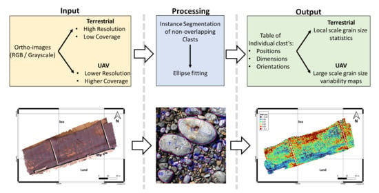
2. Data and Methodology

2.1. Data

The methodology developed uses photographs taken at human height, which include a quadra structure of known shape and dimensions (0.84 × 0.84 m²) placed on the ground. The dataset thus created includes images taken from a bird’s eye perspective, between 1.5 and 2 m high without a tripod (Figure 1a) and using two different cameras (Nikon D3200 and Apple iPhone 11). These images are corrected for lens distortion effects using a camera calibration model [33] and then ortho-rectified by planar transformation within the quadra, with a resolution fixed at 0.5 mm/pixel (Figure 1b). This fixed value was set for consistency purposes as the unprocessed image resolution can vary from about 0.25 mm/pixel for a Nikon D3200 camera to about 0.5 mm/pixel for an Apple iPhone 11 camera. Each quadra is associated with the geographical coordinates of at least one of its corners, measured in situ using differential GNSS.

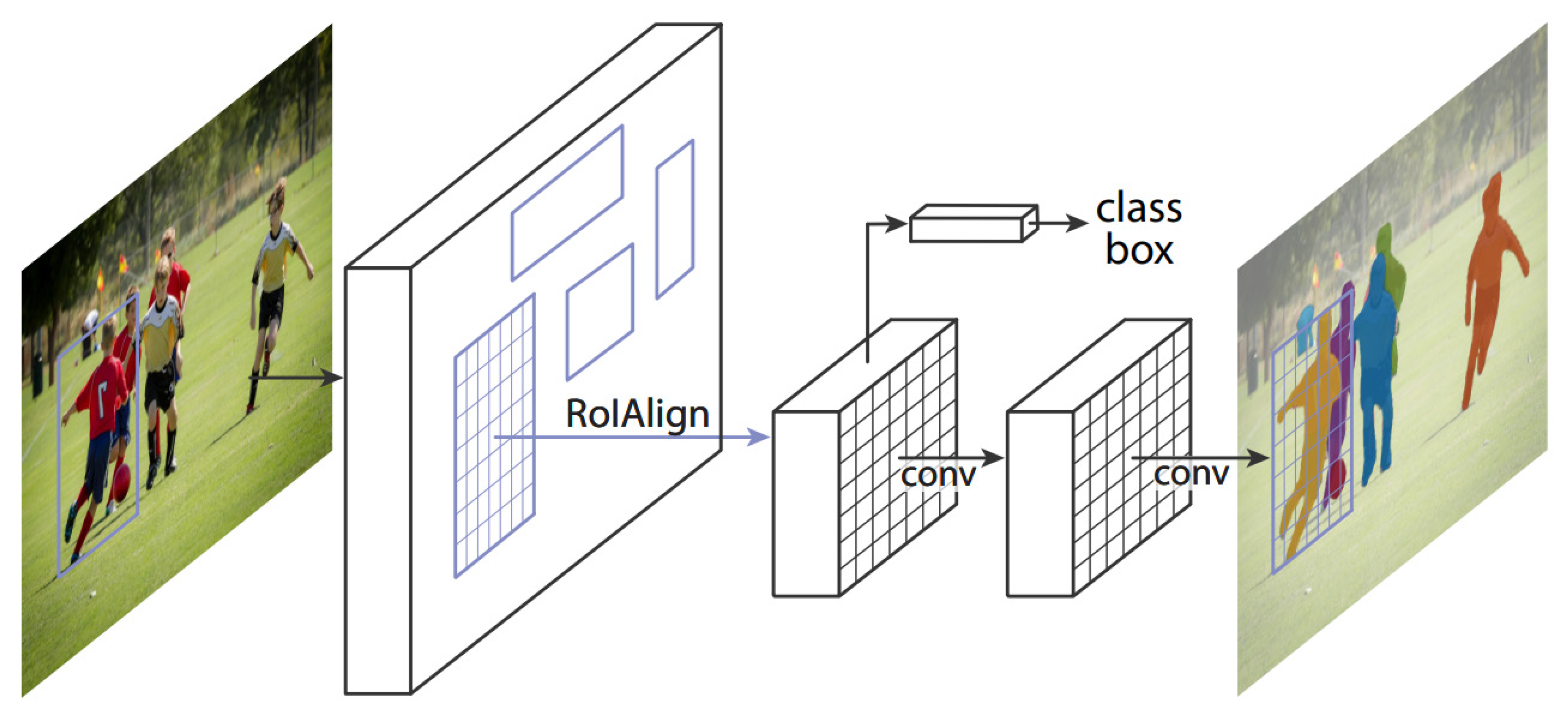
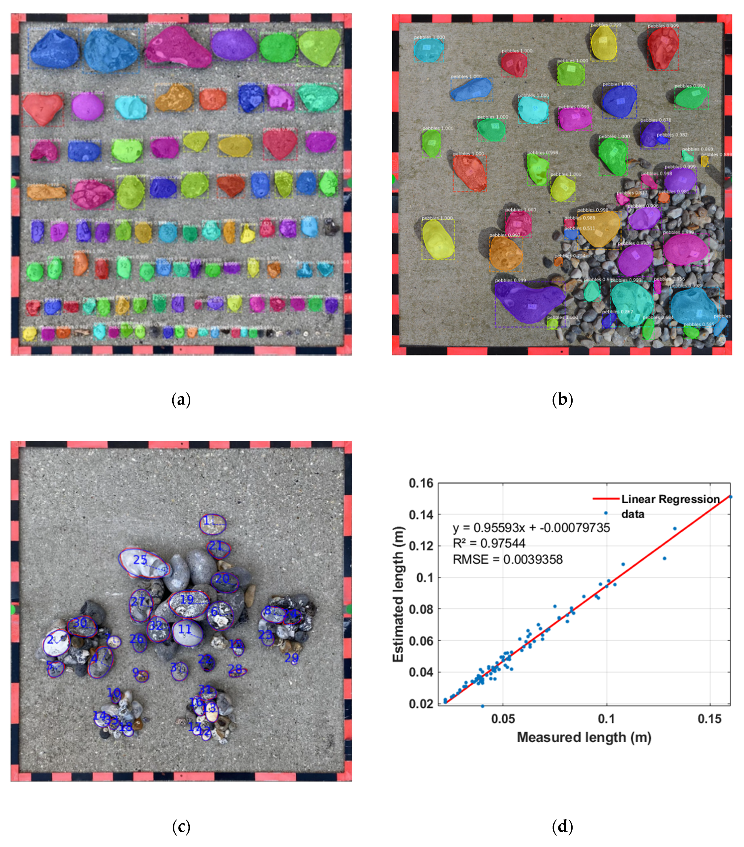
2.2. Mask R-CNN Segmentation

The algorithm that was chosen to perform the clast identification is called Mask Regional Convolutional Neural Network (Mask R-CNN). This meta-algorithm was developed by He et al. (2017) [32] and combines the proven object detection algorithms Faster R-CNN [34], which allows the identification of the nature (e.g., person, boat, car, etc.) and position of objects within bounding boxes (i.e., frame inside an image), and the Fully Convolutional Network (FCN) [35], which allows semantic segmentation, a pixel-scale classification (Figure 2).
The choice for this algorithm in particular was encouraged by the fact it was made freely accessible on various online platforms and easy to use without the need of a deep expertise of its complex working process. In addition, the algorithm is supported by a wide community of users and is densely documented through numerous technical notes and tutorials.
The working process of the Mask R-CNN can be described as a two-stage process. The goal of the first stage consists of scanning the image in order to find areas likely to contain an object, called “anchors”. These anchors will then feed the second stage, whose objective is to perform both an object detection and the classification of each pixel within the detected object’s boundary box. As a result, the model produces a series of binary masks, each of them representing the pixels that belong to a certain object. It is important to understand that in one image, every object of the same nature will have its own dedicated mask, thus making it possible to distinguish each individual instance.
As described by He et al. [32] in their article dedicated to Mask R-CNN, the first stage generates anchors using a backbone composed of a ResNet101 and a Feature Pyramid Network (FPN) that extracts the spatial information, then a Region Proposal Network (RPN) is responsible for generating random regions of interest (ROI), and then ranks their relevance according to the results of the backbone.
The second stage classifies the proposals from the first stage and generates bounding boxes and bounding masks in parallel. This is made possible by an ROI classifier which performs object detection (nature and bounding boxes) on the anchors, in order to extract the ROI. ROIs are then scaled to the fixed size of 28 pixels × 28 pixels which corresponds to the dimensions of the convolutional neural network, in order to perform a semantic segmentation on each of them and obtain a mask. Finally, the mask is resized to the initial object scale, and repositioned on the image.
The model was trained with a dataset of 46 images and a total of 3598 manually digitized non-overlapping clasts. This dataset covers as wide a range of environmental conditions as possible with elements of all sizes (from gravels to cobbles), shapes and colors, low to high light, humidity and silting conditions, presence or absence of quadra, ground and Unmanned Aerial Vehicle (UAV) shots, raw or ortho-rectified. This dataset was artificially augmented in order to improve learning performance [36] which means that some images randomly selected in the dataset were copied and transformed (addition of blur/noise, crops, rotations/translations, etc.) using random parameters, in order to artificially increase the dataset’s size. As the training step of a deep learning model works by iterations called epochs subdivided into steps, it is relevant to mention that a total of 100 epochs, each including 100 steps, was required to achieve a satisfactory segmentation capability.
After processing an image of clasts, the output of the model is recorded as a series of masks, one per detected element, each of them being associated with a probability value reflecting the certainty of the model to have correctly detected and segmented the object.
In general, the segmentation of a quadra image by the Mask R-CNN model takes 3 s on a mid-range computer (Intel® Core™ i7-8850H CPU 2.6GHz, 32GB RAM, NVIDIA Quadro P600 GPU). From one image to another, this duration can vary between 1 and 10 s depending on the amount of clasts, the initial resolution, and the computer capabilities.

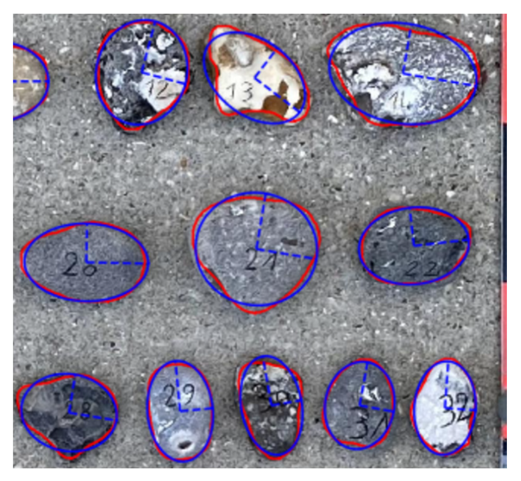
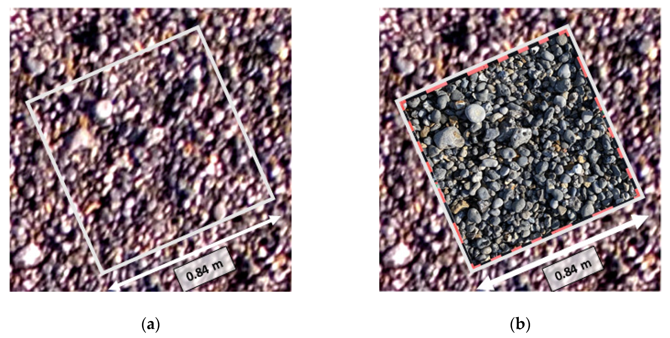
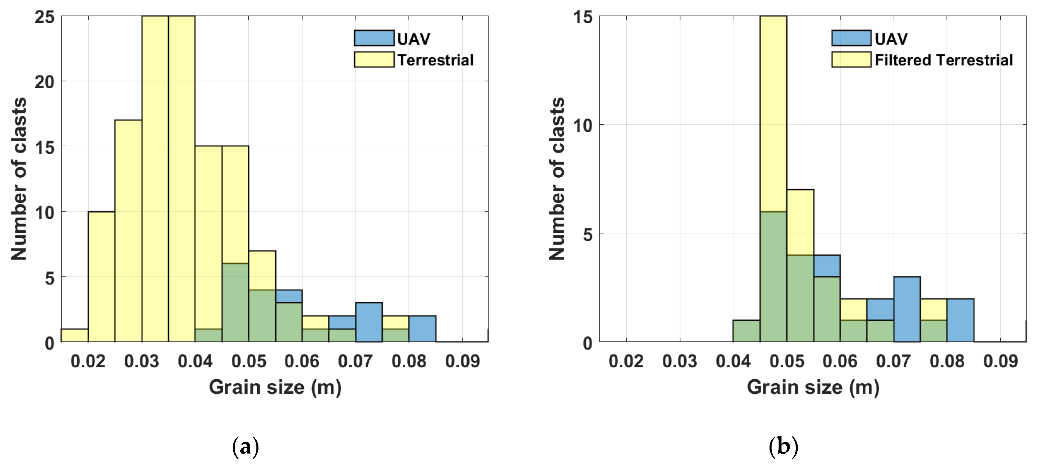
2.3. Clast Size Measurement and Validation

The clasts are measured on images with known resolution (0.5 mm/pixel). After detection of non-overlapping features by Mask R-CNN, each particle is measured along the major and minor axes of the ellipse on which they lie (Figure 3). It is important to mention that the actual particle shape is flattened by the photographing process, and therefore only two of the three dimensional axes of the sediment particle remain available, often referred as “long” and “intermediate” axes. This loss of a dimension by projection is also likely to be a source of slight errors, especially as the ellipse’s major and minor axis may not exactly equal the particle’s long and intermediate axes, although they will remain close. It is also possible to record the unprocessed mask characteristics, such as the probability value attributed by the algorithm, the area size or the full contour shape detected by Mask R-CNN for further morphological analysis.
To validate this method, the three dimensions of a set of 105 clasts were measured using the methodology developed in this paper (Figure 4a). The same clasts were then measured manually using a caliper with a millimetric precision, along the same axes as the ones positioned by the ellipse fitting step. These pebbles were originally sampled on the beach of Hautot-sur-Mer, they were naturally water-worked by the sea, and were chosen in order to show as wide a variability of sizes, shapes and colors as possible while remaining small enough in to fit in the quadra’s frame. The colors displayed in Figure 4a and 4b are numerical masks highlighting the algorithm’s detection results.
The results show an average detection rate of 80 to 90% of the non-overlapping individuals, regardless of their arrangement (Figure 4a–c), with a R2 of 98% and an RMSE of 3.9 mm, i.e., 8 px (Figure 4c). Most undetected objects have a long axis of less than 2 mm, i.e., 4 px, and are among the smallest sediment particles that were measured. Other methods relying on the segmentation of photographs of quadra structures show a minimal detection threshold ranging between 8 and 23 mm [19,26,27,28,37]. On rare occasions, Mask R-CNN misclassifies partial clasts as complete ones. Among the 269 sediment particles detected through the 11 overlapping scenarios tested, only 10 individuals (the same ones in most cases) were misidentified as non-overlapped sediment particles while being overlapped, resulting in a misidentification score of 3.7%. Figure 4c shows the validation scenario presenting the highest number of misidentified features: elements n°4 and n°25.
This validation methodology was applied under different light (with and without shadows) and background conditions (asphalt, concrete, wood, dry/wet surfaces …), with numbers written either directly on the surface of the clasts or on glued pieces of papers, with similar results. It is important to note that the model can perform a satisfying classification of these images despite the fact that it was not trained using such data, thus enforcing the model’s applicability.

3. Example of Applications
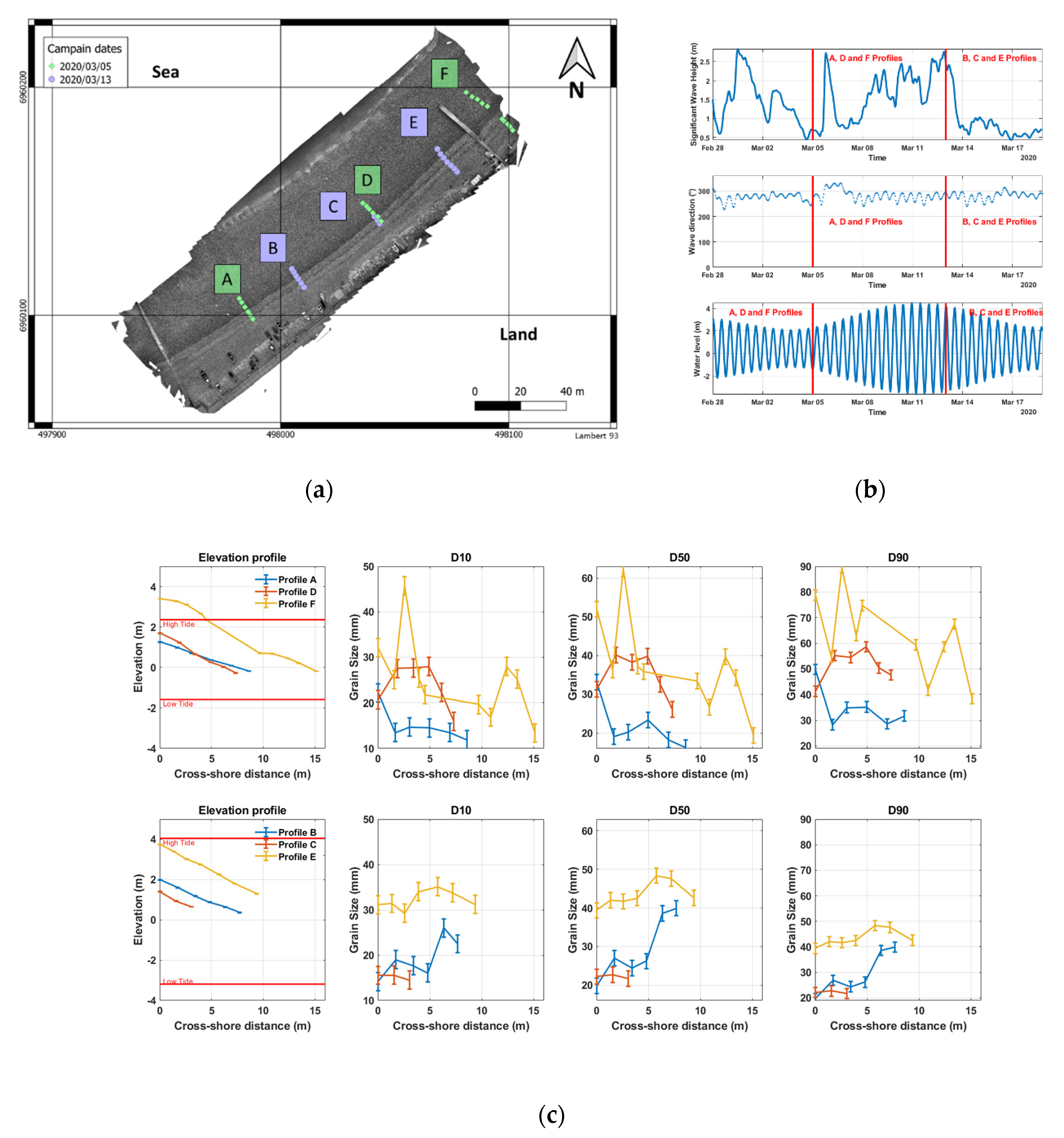
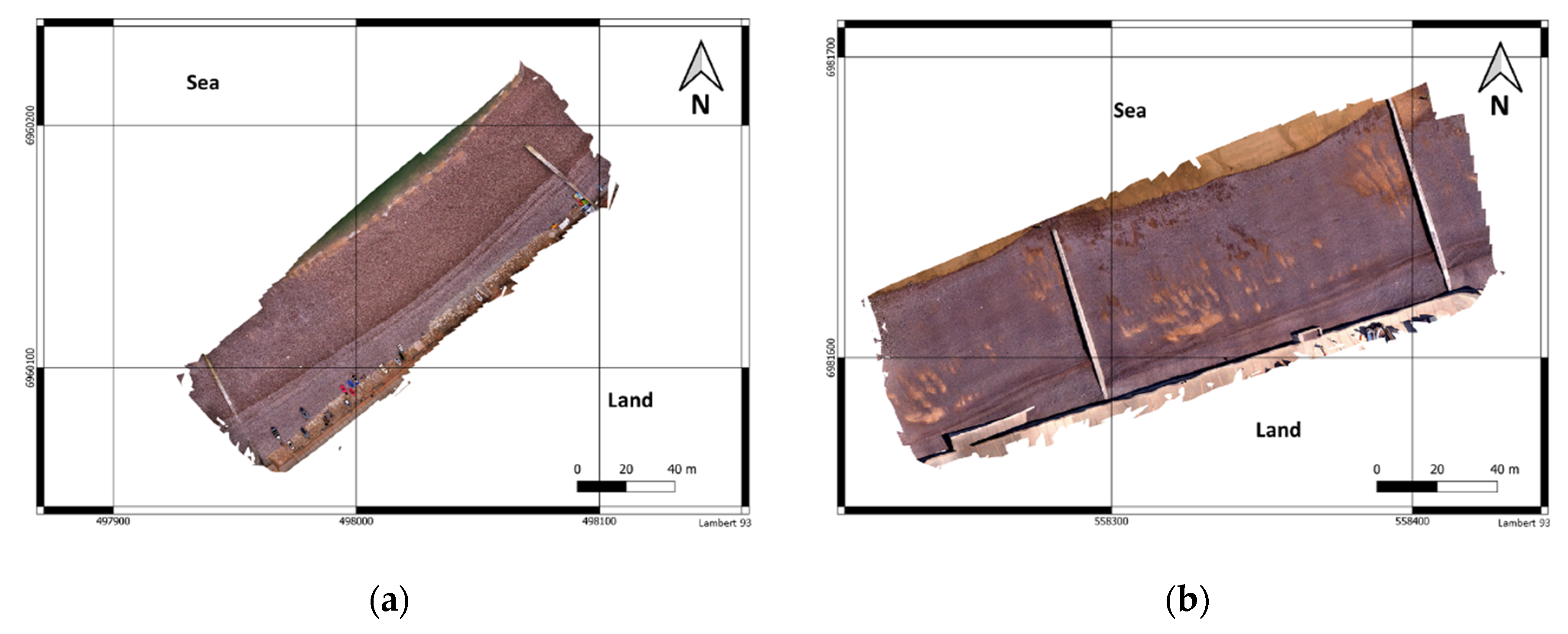
To show the potential and capabilities of the methodology developed here, this section presents two examples of analysis: The evolution of Etretat’s pebble size under different wave conditions measured using a quadra on cross-shore profiles, and the pebble size spatial variability at the scale of a large section of the beach, measured on ortho-images of Etretat and Hautot-sur-Mer (Figure 5).

3.1. Study Sites

The coast of Normandy (France) faces the English Channel, which is bordered by France to the south and England to the north. The channel forms a funnel whose width decreases from west to east. Due to this morphology, the tidal amplitudes and currents are significantly amplified on the French coasts, making the region’s coastal systems quite singular at the global scale with observed tidal ranges of up to 10 m.
The particular morphology of the English Channel also influences the impact of storms by directing winds and swells towards preferential directions, thus constraining the associated wind fetches: W–E (infinite wind fetch), NE–SW (550 km wind fetch), NW–SE (200 km wind fetch), N–S (100 km wind fetch) [38]. Cerema (2020) [39] observed extreme wave significant heights (Q99) of 2.96 m at Antifer, Etretat area, and 2.6 m at Dieppe, near Hautot-sur-Mer.
In Normandy, pebbles constitute an important part of the coastal sedimentary stock. They result from the erosion of limestone cliffs by meteorological and marine forces. The geological strata of flint fall at the foot of the cliffs, then the fragments are rolled and rounded under the waves’ action. The pebbles thus formed are then transported in a long-shore movement depending on the direction of the swells. The main direction of transport is northeastward. In calm conditions, the pebbles settle and accumulate near estuary mouths, in the hollows of bays and at the foot of obstacles to the longshore drift such as cross-shore defensive structures. The pebbles then form sedimentary bodies including pebble bars, barriers and ridges.
During a storm, much of the wave energy is dissipated by the pebble’s movements and thus the erosion of the ridge, which has the advantage of protecting coastal structures and activities. As with any non-cohesive sedimentary body, the erosion and accumulation characteristics of the pebble ridge depends on the intrinsic parameters of its constituent elements. Thus, pebble size is expected to play a major role in the morphological dynamics of pebble beaches.
During this work, two study sites were analyzed: Etretat and Hautot-sur-Mer (Figure 5). Both are touristic beaches characterized by the presence of a pebble ridge resting at the foot of a seawall and crossed by groins.
Hautot-sur-Mer is a 1000 m long semi-open system located at the mouth of the Scie Valley. The chalk cliffs that surround it show an average retreat of 20 to 50 cm per year [40], regularly replenishing the stock of pebbles. The ridge at the front of the seawall is formed by pebbles that are 5 to 10 cm in size, which are trapped in the middle of seven cross-shore groins. According to the classification of Jennings and Shulmeister (2002) [41], the site corresponds to the definition of a composite beach: the ridge (slope > 10%) lies on a sandy substrate (slope 1.3%) which can emerge over more than 210 m at low tide. Four kilometers to the east is the town of Dieppe, whose harbor is protected from the transit of pebbles at its entrance by a 500 m long pier. This structure accumulates a large part of the regional stock of pebbles.
The Bay of Etretat is a 1000 m long enclosed system, framed by high cliffs made of more indurated limestone (average retreat of between 14 and 17 cm/year [40]), forming capes that block the longshore drift. The pebble stock is old, elements are smaller in size (2 to 10 cm) and few are mobilized by coastal transit because they are trapped in the bay. This stock accumulates in the form of a pure pebble ridge [41] (10% slope) installed against the seawall of the four groins, with a cross-shore extension of up to 150 m at lowest tides.
Although the characteristics of the two sites are different, there are common morphological features such as the presence of steps and cusps and the intermittent appearance of sandy areas on the surface of the foreshore part of the beach.

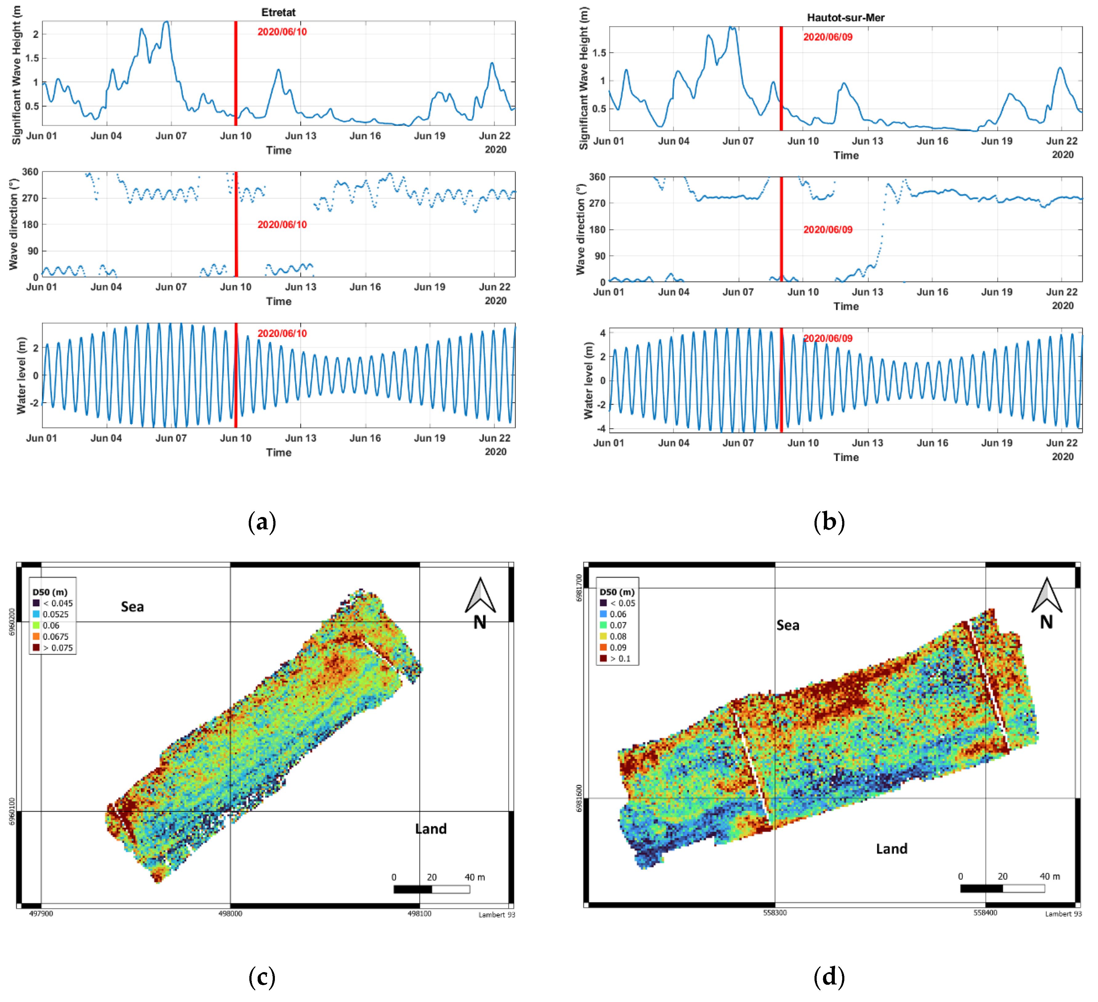
3.2. Influence of the Hydrodynamics on Etretat Pebbles’ Size

Two campaigns of pebble size measurements by quadra were carried out in Etretat one week apart in March 2020. Three profiles (Figure 6a) were recorded during each campaign: A, D and F on March 5 and B, C and E on March 13, including one common profile: C and D.
Figure 6b shows the evolution of the significant wave height and origin direction as well as the water level estimated by the WaveWatch III model off Etretat during the studied period. The March 5 measurements were carried out in a rather calm hydrodynamic context with western waves of less than one meter in height during the five days preceding the measurement, during spring tide. On March 13, more agitated conditions were observed, with waves reaching more than 2.5 m in height coming from the west during the four days preceding the campaign at neap tide.
The sediment size used for this analysis was the length of the ellipse’s major axis that provided the best fit to each object. Figure 6c shows the pebble size results from previously mentioned measurement campaigns. The topographic profiles are presented on the left, along with the vertical extension of the latest tide. The origin of the x-axis is taken at the most upstream point of each profile. The smaller extension of the profiles on 13 March is explained by a larger tidal range that constrained the measurement area.
In general, values of D10, D50 and D90 observed at Etretat vary between 1 cm and 5 cm, between 2 cm and 6 cm, and between 3 cm and 6.5 cm, respectively, all dates combined. Among all measurements, only the five first ones located on the top the F profile are at a higher elevation than the latest high tide and were therefore not affected by the tidal dynamic during the few days to weeks before 5 March, 2020.
There is a greater elevation in the east than in the west, with, for example, profile A being lower than profile F, and with a similar relationship between profiles B and E (Figure 6c). This elevation reflects a greater sediment accumulation in the east due to the long-shore sediment transport phenomenon. The grain size evolution follows the same trend, with larger sizes also in the east for higher elevations (Figure 6c), which suggests the presence of a relationship between elevation and pebble size.
However, while a negative upstream to downstream gradient is observed on all profiles on 5 March, the gradient becomes positive on 13 February. The significance of the slopes was tested using a Mann–Kendall test (Table 1). All pebble size profiles from 5 March, 2020 show an upward trend, while all those from March 13 are downward, although only 6 of the 18 size class profiles (6 × D10 + 6 × D50 + 6 × D90) show a significant trend (p-value < 0.1) due to the low number of measurement points.
On the other hand, the D90 decreases significantly between 5 February and 13 February, from an average of 5 cm to 3 cm. In particular, the comparison of profiles C and D shows a decrease in all three indices.
Previous studies carried out by the Laboratoire Central d’Hydraulique de France (LCHF) [42] show that for 15 pebble ridges along the Normandy coastline, there is a tendency for the pebble size to decrease from upstream to downstream, with a D50 in particular evolving from 4 cm to 5.5 cm at Etretat. These values correspond to the range of lengths measured during this study: between 2 and 6 cm.
Other authors such as Bujan et al. [43] found a similar positive correlation between beach elevation and coarse clast size to the one found for profiles A, D and F (Figure 6c), while surveying a pebble beach in Taiwan’s region using an analogous methodology. However, the works of Costa et al. and Letortu [38,44] show that pebble size can have significant spatial variability at the tidal cycle scale, depending on the marine conditions preceding the observation. Other comparable studies do not seem to find any evident linear relationship between elevation and grain size [45]. The results presented here support this observation and show that particle size sorting can be positively or negatively correlated with elevation depending on the previous wave conditions.
These observations are in good alignment with previous studies’ findings about clast transport in the swash zone under different energetic conditions. Under calm wave conditions, the asymmetrical balance between the uprush and the backwash energy tends to carry more material upslope than downslope, which eventually leads to an accumulation of sediment on the surface of the beach [46]. When the wave height the reaches a certain threshold in the swash zone, the processes of infiltration and percolation are not able to completely dissipate the wave energy anymore, and the swash becomes saturated [47,48,49]. For such energetic wave conditions and higher ones, more sediments are carried downslope and eventually dispersed until the occurrence of calmer conditions that will allow the beach to grow again. The coarser sediments are then expected to be transported at a slower pace than the finer ones, as their transport will require more energy. This difference in transport speed is expected to sort the surface sediment by size. This hypothesis is supported by previous studies that highlighted the existence of such seaward shift, the direction of which has been found to rely on a wave height threshold [45,50,51]. When associated with the alternance between spring and neap tide, one can understand that the previously mentioned accumulating conditions associated with spring high tides are likely to store and preserve the sediment on the backshore, at elevations that are only reached by the sea during spring tides and/or storms.
If the previous accumulating conditions lasted long enough, a significant amount of the largest clasts, previously found downstream, could have been transported on the backshore and been preserved from the neap tide storm of February 29 (five first measurements of profile F, Figure 6c), resulting in the upstream to downstream negative grain size gradients observed on March 5. Although the saturation wave height threshold is unknown for Etretat, it is fair to assume that such conditions were reached shortly before the measurement campaign of March 13. Therefore, the clasts located at higher elevations were dispersed, which lowered the grain size quantiles and reversed the gradients.

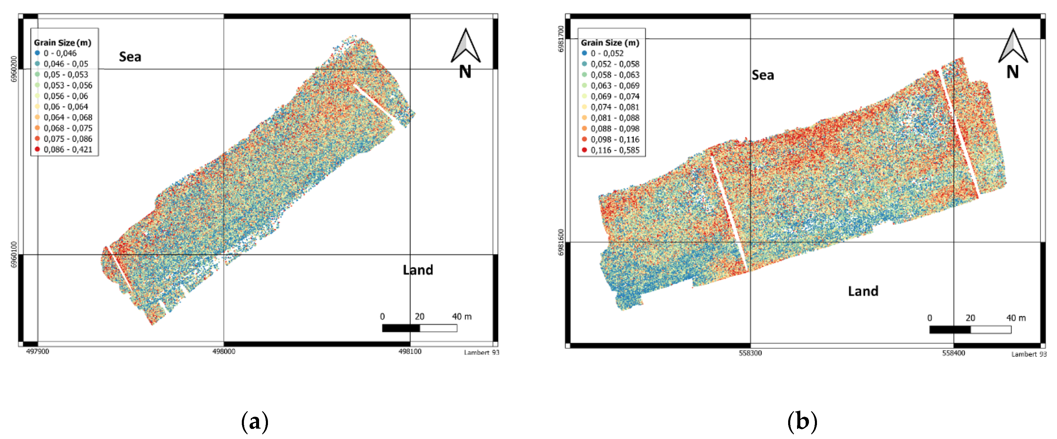
3.3. Clast Size Mapping at Etretat and Hautot-Sur-Mer
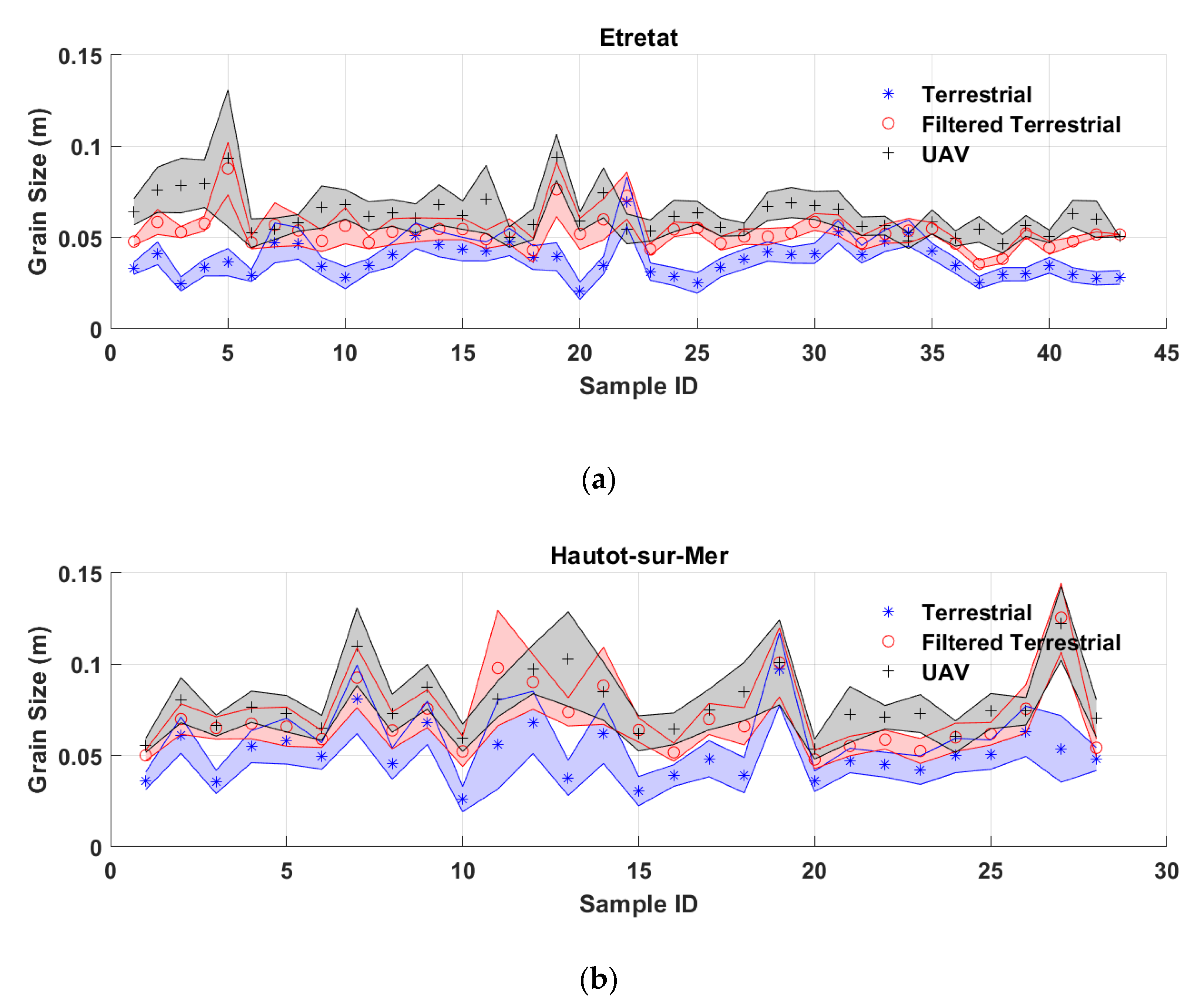
Two UAV campaigns were carried out in Hautot-sur-Mer and Etretat on June 9 and June 10, 2020. These campaigns made it possible to create ortho-images at the scale of the beach, with a resolution of 5 mm/pixel covering 9000 m2 at Etretat (Figure 7a) and 12,000 m2 at Hautot-sur-Mer (Figure 7b) using Surface From Motion (SFM) techniques. On both sites, the flight was carried out using a DJI Inspire 1 with a Zenmuse X5 camera (image size = 4608 pixels × 4608 pixels; sensor size = 17.3 mm × 13 mm; Focal length = 15 mm). Flights were attended at a fixed altitude of 20 m above the top of the beach, with an increase due to the beach slope up to 30 m at Hautot-sur-Mer and 35 m at Etretat. Therefore, the expected Ground Sampling Distance (GSD) values range from 5 to 7.5 mm/pixel at Hautot-sur-Mer, and from 5 to 8.8 mm at Etretat, and are correctly oversampled by the image resolution of 5 mm/pixel.

3.3.1. Validation

As the size of the image that can be input into the Mask R-CNN algorithm is limited for computational reasons, the ortho-images were cut out into tiles of 1 × 1 m² in size (Figure 8), to be analyzed one by one. Although convenient, the fixed size of 1 × 1 m² constrains the size of the detectable objects to smaller dimensions. Once detected, the pebble coordinates and dimensions are stored in an output table file containing all the previously detected pebbles of the entire ortho-image. The overall process takes around one day per ortho-image.
Since the validation results presented in Section 2.3 showed that measurements by quadra were accurate and reliable, here they were considered as ground truth data for validation purposes. Therefore, some were carried out in parallel with the flight of the UAV to allow cross-validation of the results. A total of 46 and 28 quadra measurements were realized at Etretat and Hautot-sur-Mer, respectively, covering the whole surveyed area on both sites.
Validation is performed by comparing each quadra distribution (here called “terrestrial samples”) to the one being extracted at the same location from the ortho-image, on areas covering 1 × 1 m² so called “UAV samples”, considering the terrestrial samples as ground truth. It is important to understand that this validation process only compares distribution indices (quantiles, means, etc.), as the automatic cross-identification of individuals on both datasets remains a challenging task.
On the ortho-image segmentation, smaller objects are expected to be under-represented, due to the lower resolution in comparison to the quadra data (0.5 mm/pixel) (Figure 9a,b).
Therefore, the distribution measured on the ortho-images reflects the tail of the distribution measured with quadra (Figure 10a). In order to compare both types of datasets as relevantly as possible, the clasts detected in the terrestrial samples were filtered. The filtering operation consists of eliminating the pebbles that are smaller than a defined threshold in each terrestrial sample. This threshold is set to be the size of the smallest object detected in the UAV samples of the same location. When filtered out, the respective ranges of the results and the number of detected pebbles per area unit of the two datasets correspond to what is expected: more small elements are found in the filtered terrestrial samples, and similar amounts are detected for the bigger ones (Figure 10b).
Figure 11a,b show the distributions (before and after filtering) of the clasts from the terrestrial samples as well as the distributions from the UAV samples, at Etretat and Hautot-sur-Mer, respectively. For the vast majority of samples, the filtering operation brings the terrestrial means significantly closer to the UAV sample ones, regardless of the site, which shows the relevance of this operation.
The variability of the mean values from one sample to another is similar between filtered terrestrial and UAV samples. This shows the ability of the method to produce relevant distributions above a certain threshold. According to the minimum size limit of four pixels found in Section 2.3., this threshold should be 2 cm with 5 mm/pixel resolution. However, elements under 4 to 5 cm in size remain difficult if not impossible to identify on ortho-images. This tends to show that the overall GSD is closer to 10 mm/pixel or higher. This seems to be aligned with the calculated values ranging between 5 and 8.8 mm/pixel considering the eventual potential additional loss of resolution due to the SFM processing.
The quantiles–quantiles diagrams (Figure 11c,d) highlight a quasi-linear relationship between the filtered terrestrial and UAV sample quantile classes, although the UAV samples slightly overestimate these values.
Figure 11e,f show the comparative distributions of mean sizes between filtered terrestrial and UAV samples. The R2 values of 0.45 and 0.75 and RMSE values of 6.8 mm and 9.3 mm at Etretat and Hautot-sur-Mer, respectively, confirm the ability of the present methodology to determine the size of pebbles on ortho-images. The lower R2 at Etretat (Figure 11e) and the regression line’s slope of 0.56 seem to be associated with the small range of sizes, the majority of samples measuring between 43 and 59 mm. Although the precision is expected to be ± eight pixels, (i.e., ± 4 cm for 5 mm/pixel resolution), the calculated RMSE values suggest an uncertainty of only one to two pixels. This tends to show that the relationship between the Mask R-CNN detection uncertainty and the image resolution is not linear. Indeed, assuming that the model was sufficiently trained, Mask R-CNN will only delineate the elements that are likely to be actual clasts. Therefore, for a given image, a decrease in the resolution will result in a lower number of detected elements and a higher smallest element size, with a similar size measurement accuracy only increased up to the pixel size.
It is expected that the measurement error on the ortho-images is higher downstream than upstream as the UAV evolves on a horizontal plane above the inclined plane of the pebble ridge. The greater observation distance above the beach’s downstream area implies a higher GSD value. An increase in absolute error is indeed observed with the increase in observation distance of about 0.8 mm per meter of elevation at the two study sites (Figure 11g,h). The statistical significance of these trends was tested by a Mann–Kendall test and shows p-values of 0.05 and 0.24 at Etretat and Hautot-sur-Mer, respectively. However, the R2 values of 0.11 and 0.05 remain low and highlight the variability of the absolute error, which is on average less than 1 cm, but can reach almost 3 cm at times.
These observations confirm the good capability of this methodology to map the spatial variability of pebble size in a relevant way.

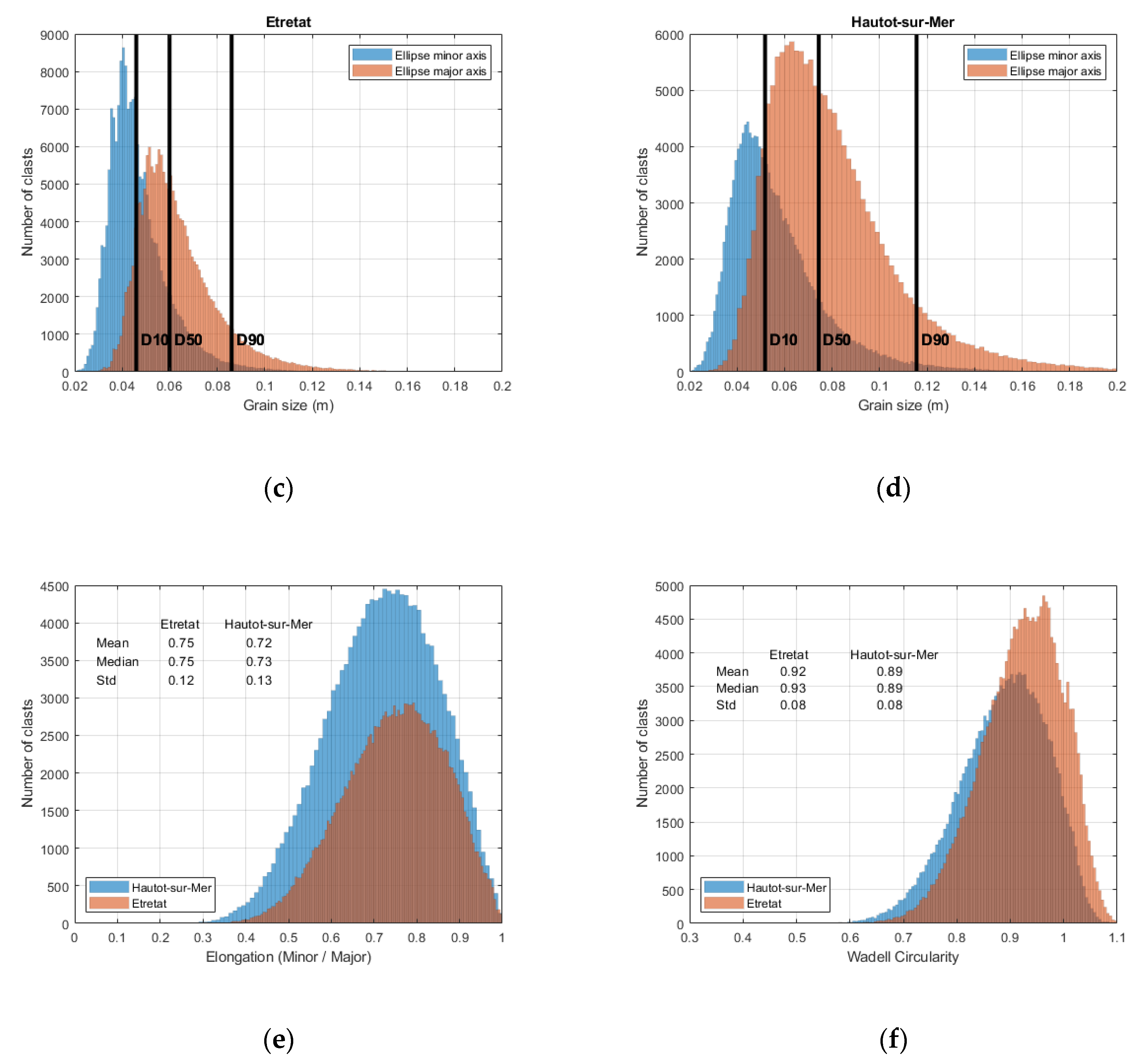
3.3.2. Results and Discussion

A total of 182,218 clasts were detected on Etretat beach (Figure 12a) with a D10 of 4.59 cm, a D50 of 5.99 cm and a D90 of 8.6 cm. At Hautot-sur-Mer, 153,824 clasts were detected (Figure 12b) with a D10 of 5.18 cm, a D50 of 7.44 cm and a D90 of 11.55 cm (Figure 12c,d). These clast size values are similar to those measured by LCHF [42], although the D10s measured here are slightly higher by about 1 cm. The minimum dimensions are similar on both sites with around 2 cm and 3 cm for the minor and the major axis, respectively (Figure 12c,d). On the contrary, maximum values differ with about 10 cm and 15 cm for the minor axis, at Etretat and Hautot-sur-Mer respectively, and about 13 cm and more than 20 cm for the major axis. However, these values are not to be considered as the actual observed maxima due to the 1 × 1 m² cropping window used for the detection that is likely to have cut the boulders of similar or larger dimensions, which are therefore not detected.
A quick analysis of the elongation and circularity was made possible by the availability of a major and a minor axis dimension for each sediment particle. The elongation was calculated by the ratio ellipse minor axis over major axis [52], and provides results ranging from zero (infinitely long particle) to one (the major axis equals the minor axis). For circularity, the Wadell’s [53] definition was considered and calculated by the ratio between the particle’s equivalent diameter (i.e., diameter of the circle that equals the surface of the detected sediment particle mask) and the ellipse major axis. Circularity values are expected to range from zero to one (i.e., ellipse like shapes to circle like shapes).
Figure 12e presents the histogram of elongation values found at Etretat and Hautot-sur-Mer. Results show similar elongations on both sites with a lower average value of 0.72 at Hautot-sur-Mer as compared to 0.75 at Etretat. Figure 12f shows the histogram of circularity values. As expected for wave-worked sediment material, values stay close to one for both sites with 0.92 at Etretat and 0.89 at Hautot-sur-Mer on average. This also tends to show that Etretat’s pebbles are typically rounder than Hautot-sur-Mer ones. Values superior to one are likely to show the limits of the ellipse fitting process which could produce ellipse axis dimensions being slightly smaller than the actual sediment particle dimensions.
At both sites, the measurement campaign took place during a mildly agitated hydrodynamic period (hs < 1 m for several days) in the presence of a N–NW swell at the end of the spring tide (Figure 13a,b). A week before, these campaigns were preceded by a more energetic event with waves up to 2 m in height on both sites, during the spring tide peak.
After the Mask R-CNN detection processing, detected sediment particles sizes were rasterized in order to be analyzed in an easier way (Figure 13c,d). The present rasters were produced by finding the quantile 50 of each cell of a grid of 1 × 1 m² in size covering the beaches.
In general, the results show a positive upstream to downstream particle size gradient over both ridges (Figure 13c,d). This observation contradicts the systematic negative gradient measured by LCHF (1972) [42] but both types of observation can be explained with the mechanism described in the Section 3.2.
However, this gradient is very heterogeneous, with preferential areas of coarser or finer sediment accumulation. On Figure 13c, Etretat’s beach shows a specific accumulation spots with sediment larger than 6.7 cm on the northeast part of the beach face. Other spots can be identified along the groins, especially around their tip, with even higher sizes. On the contrary, the back of the beach is characterized by finer grains of 4.5 cm in size and less. Longshore oriented patterns can be identified along the different berm slopes.
On Figure 13d, the beach of Hautot-sur-Mer presents a more contrasted picture, with similar observations. Interestingly, the same observations can be made in the two visible sections of beach that are embayed by the groins, although the western one is only partial: the presence of two distinguishable patches of high values (D50 ⩾ 9 cm) on the west side of the groins, one on the beach’s top, the second one more towards the center; another wider area of high values (D50 ⩾ 9 cm) is located along the front of the beach; the eastern side of the beach front is showing significantly lower values (D50 ⩽ 6 cm) with some a high local variability (punctual D50 ⩾ 10 cm); the top of the beach is also an homogeneous area of low values (D50 ⩽ 6 cm); the eastern side of each groin seems to accumulate a mix between moderate (6 cm ⩽ D50 ⩽ 9 cm) and high values (D50 ⩾ 9 cm); the rest of the beach face presents homogeneous moderate values (6 cm ⩽ D50 ⩽ 9 cm).
Other more specific observations tend to show effects of the slope on sediment size sorting, and the interactions between the sediment and the defense structures, such as the groin’s ability to capture the larger elements.
Based on the occurrence of an energetic event during the spring tide peak, a week before the measurement campaign, the observed negative upstream to downstream gradient of D50 can be explained by the same mechanism as the one mentioned in Section 3.2. When the spring tide amplitude is able to completely flood the beach, highly energetic conditions are likely to disperse pebbles of all sizes if the wave height is superior to a saturation threshold [47,48,49]. While this value remains unknown for the beaches of this study to this day, it seems reasonable to assume that it was reached on June 6 for both sites. Therefore, under fairer weather conditions, the beach is expected to grow back thanks to the one-way swash transport associated with the high tidal amplitude. During this mechanism, larger clasts are likely to be transported at a slower pace than the finer ones, resulting in a temporary negative gradient. If such calm conditions remain, one can expect to see the upstream D50 increase back, and even reach a positive upstream to downstream gradient.

4. Discussion

Mask R-CNN allows the satisfactory segmentation of uncovered clasts on an image. On close range images with a quadra structure for scale, the clasts are correctly segmented when their dimensions are greater than 2 mm, with an uncertainty of ± 4 mm (for a resolution of 0.5 mm/pixel). On orthoimages, it was possible to obtain a satisfactory detection of the sediment particles greater than 4 cm with an uncertainty of ± 6.8 mm at Etretat and 9.3 mm at Hautot-sur-Mer. The minimal size threshold value was shown to strongly depend on the GSD (tested values of 0.5 mm/pixel for the terrestrial images, and 5 to 8.8 mm/pixel for UAV images) while the uncertainty ranges between 4 and 9.3 mm. The processing time of a few seconds per square meter of image (numerical resolution between 0.5 and 5 mm/pixel), along with the ability of the model to function without human supervision are valuable assets.
Although more precise, the terrestrial technique remains more punctual and therefore provides less spatially representative results than the UAV method. Moreover, in time constrained environments such as semi-diurnal intertidal areas, the efficiency of the UAV methodology potentially allows the investigation of larger domains. Nevertheless, it has been proven possible to combine both methods’ strengths in order to provide reliably validated results.
The methodology described in the present article has shown the tool’s strong performance when monitoring the spatial and temporal evolution of the pebbles’ size on two pebble ridges.
The results obtained show the evolution of the beach’s D50 upstream to downstream gradient as a function of the hydrodynamic conditions. They support the hypothesis of a multi-factor process at the origin of the seaward sorting gradient as it was observed to be negative at neap tide before a storm in Etretat, then positive at spring tide after a storm. Furthermore, positive gradients were observed at Etretat and Hautot-sur-Mer after a spring tide storm.
The acting mechanism relies on the supposition that the swash saturation threshold [47,48,49] was reached during the spring tide energetic events preceding the measurements, thus eroding and dispersing the beach’s top sediment. Under calmer conditions, this sediment accumulates again, each element moving at a speed that is proportional to its size, which results in the appearance of surface sediment sorting patterns. These observations and explanations are supported by several comparable other studies conducted on different coarse clastic beaches, with similar conclusions about a seaward grain size shift whose direction depends on a wave height threshold [45,50,51].
In a more specific perspective, the results highlight the effect of the beach slope and of the groins on the particle size sorting, with an accumulation of the coarsest elements at the around the structures. The presence of similar patterns in side by side groin embayed beach sections once again confirms the relevance of the method by showing its ability to produce consistent measurements for consistent sorting conditions.
These results therefore provide a better understanding of the coastal pebble system dynamics. In Normandy, these results will be used to feed a model of the morpho-sedimentary evolution of beach pebble barrier beaches, and thus provide a better understanding of the sedimentary dynamics at work in the extreme tidal conditions of the region.

5. Conclusions

The Mask R-CNN model is a versatile instance segmentation method that has proven its performance in many areas, and is particularly suitable for clast size measurement applications for several reasons. First, convolutional neural networks are useful for the classification of non-trivial concepts, such as non-overlapping pebbles. This capability allows the minimization of sampling bias by disqualifying partially visible objects. In addition, the processing speed associated with the tool’s ability to operate without human supervision after image scaling makes it a remarkably efficient asset.
The methodology developed for this study is validated with an uncertainty of ±8 pixels (±4 mm for a resolution of 0.5 mm/pixel) against a manually measured dataset. Part of this uncertainty can be attributed to the loss of a dimension, a photograph being the projection of a 3D scene on a 2D plane, as well as to the simplification of the morphology of the pebbles into ellipses. However, the measurement uncertainty does not seem to increase much with the decrease in the image resolution (RMSE of 6.8 to 9.3 mm for images with 5 mm/pixel of resolution), as the algorithm will not detect unclear features.
This methodology was applied as an example to Normandy beaches made up of pebbles on two different types of data: terrestrial photographs in top view at a height of about 2 m without a tripod using a quadra structure for scale, and ortho-images produced at the end of a UAV flight.
The results obtained are consistent with previous observations, and allow analysis of the spatial and temporal evolution of the pebble size variability at Etretat and Hautot-sur-Mer. These observations highlight the particle size sorting, and its spatial and temporal heterogeneity. The occurrence of size changes concomitant to the presence of specific hydrodynamic conditions suggests that the responsibility for sorting the coarse clasts is shared by a combination of several factors such as significant wave height and tidal amplitude. This paves the way for a better understanding of the dynamics of pebbles on the beaches of Normandy and will form the basis of further research.
Although these results have demonstrated that the method is suitable for monitoring the size of pebbles on the beaches of Normandy, the spectrum of applications remains a lot wider. Indeed, the model can be trained to classify other types of elements, and records their complete shapes and not only their size. Therefore, it is now possible to map and study the morphological characteristics of clasts and their evolution through time and space with good accuracy, low cost, and low expertise, in a relatively short time.

Author Contributions

Conceptualization, A.S.; methodology, A.S.; software, A.S.; validation, A.S., M.F. and B.P.; formal analysis, A.S., I.T., M.F.; investigation, A.S.; resources, A.S., I.T.; data curation, A.S.; writing—original draft preparation, A.S.; writing—review and editing, I.T., N.L., M.F., S.C.; visualization, A.S.; supervision, I.T., N.L.; project administration, N.L., I.T., S.C.; funding acquisition, I.T., S.C. All authors have read and agreed to the published version of the manuscript.

Funding

This research received no external funding.

Acknowledgments

This work is part of a project called EC2CO INSU RGB (Response of Gravel Beaches—N°12720) run by INSU (National Institute of Sciences of the Universe). The authors wish to acknowledge the city services of Etretat and Hautot-sur-Mer that allowed and helped this study to be conducted, and to the multimedia office of the University of Rouen Normandy for providing their UAV expertise. Moreover, the authors are grateful for Benjamin Bazin and Jackie Steele who took care of the labeling part and proofread the English version of this article (JS), and for Romain Levaillant and Michel Simon who designed the quadra structure of this study. Finally, the authors would like to express their gratitude to the editors and reviewers for the time dedicated to the peer-reviewing process of this article.

Conflicts of Interest

The authors declare no conflict of interest.

References

  1. Buscombe, D.; Masselink, G. Concepts in gravel beach dynamics. Earth-Science Rev. 2006, 79, 33–52. [Google Scholar] [CrossRef]
  2. Finkl, C.W. Coastal classification: Systematic approaches to consider in the development of a comprehensive scheme. J. Coast. Res. 2004, 20, 166–213. [Google Scholar] [CrossRef]
  3. Gomez, B. Temporal variations in bedload transport rates: The effect of progressive bed armouring. Earth Surf. Process. Landforms 1983, 8, 41–54. [Google Scholar] [CrossRef]
  4. Klingeman, P.C.; Emmett, W.W. Gravel bedload transport processes. In Gravel Bed Rivers; Hey, R.D., Bathurst, J.C., Thorne, C.R., Eds.; Wiley: Chichester, UK, 1982; pp. 141–179. [Google Scholar]
  5. Mason, T.; Coates, T.T. Sediment transport processes on mixed beaches: A review for shoreline management. J. Coast. Res. 2001, 17, 645–657. [Google Scholar]
  6. Rubin, D.M.; Topping, D.J. Quantifying the relative importance of flow regulation and grain size regulation of suspended sediment transport α and tracking changes in grain size of bed sediment β (Water Resources Research (2008) 44, (W09701) DOI: 10.1029/2008WR006819). Water Resour. Res. 2008, 44, 133–146. [Google Scholar] [CrossRef]
  7. Bergillos, R.J.; Masselink, G.; McCall, R.T.; Ortega-Sánchez, M. Modelling overwash vulnerability along mixed sand-gravel coasts with xbeach-g: Case study of playa granada, southern Spain. Proc. Coast. Eng. Conf. 2016, 35, 1–9. [Google Scholar]
  8. Masselink, G.; Poate, T.; McCall, R.; van Geer, P. Modelling storm response on gravel beaches using XBeach-G. Proc. Inst. Civ. Eng. Marit. Eng. 2014, 167, 173–191. [Google Scholar] [CrossRef] [Green Version]
  9. Dal Cin, R. “Pebble clusters”: Their origin and utilization in the study of palaeocurrents. Sediment. Geol. 1968, 2, 233–241. [Google Scholar] [CrossRef]
  10. Butt, T.; Russell, P.; Turner, I. The influence of swash infiltration–exfiltration on beach face sediment transport: Onshore or offshore? Coast. Eng. 2001, 42, 35–52. [Google Scholar] [CrossRef]
  11. Kondolf, G.M.; Wolman, M.G. The sizes of salmonid spawning gravels. Water Resour. Res. 1993, 29, 2275–2285. [Google Scholar] [CrossRef]
  12. Adams, J. Gravel Size Analysis from Photographs. J. Hydraul. Div. 1979, 105, 1247–1255. [Google Scholar]
  13. Kellerhals, R.; Bray, D.I. Sampling Procedures for Coarse Fluvial Sediments. J. Hydraul. Div. 1971, 97, 1165–1180. [Google Scholar]
  14. Barnard, P.L.; Rubin, D.M.; Harney, J.; Mustain, N. Field test comparison of an autocorrelation technique for determining grain size using a digital “beachball” camera versus traditional methods. Sediment. Geol. 2007, 201, 180–195. [Google Scholar] [CrossRef]
  15. Graham, D.J.; Rice, S.P.; Reid, I. A transferable method for the automated grain sizing of river gravels. Water Resour. Res. 2005, 41, 1–12. [Google Scholar] [CrossRef] [Green Version]
  16. Fehr, R. Einfache Bestimmung der Korngrös¬senverteilung von Geschiebematerial mit Hilfe der Linienzahlanalyse (Simple detection of grain size distribution of sediment material using line-count analysis). Schweizer Ing. und Archit. 1987, 105, 1104–1109. [Google Scholar]
  17. Leopold, L.B. An Improved Method for Size Distribution of Stream Bed Gravel. Water Resour. Res. 1970, 6, 1357–1366. [Google Scholar] [CrossRef]
  18. Wolman, M.G. A method of sampling coarse river-bed material. Trans. Am. Geophys. Union 1954, 35, 951–956. [Google Scholar] [CrossRef]
  19. Ibbeken, H.; Schleyer, R. Photo-sieving: A method for grain-size analysis of coarse-grained, unconsolidated bedding surfaces. Earth Surf. Process. Landforms 1986, 11, 59–77. [Google Scholar] [CrossRef]
  20. Buscombe, D.; Masselink, G. Grain-size information from the statistical properties of digital images of sediment. Sedimentology 2009, 56, 421–438. [Google Scholar] [CrossRef]
  21. Buscombe, D. SediNet: A configurable deep learning model for mixed qualitative and quantitative optical granulometry. Earth Surf. Process. Landforms 2020, 45, 638–651. [Google Scholar] [CrossRef]
  22. Buscombe, D. Transferable wavelet method for grain-size distribution from images of sediment surfaces and thin sections, and other natural granular patterns. Sedimentology 2013, 60, 1709–1732. [Google Scholar] [CrossRef]
  23. Carbonneau, P.E.; Lane, S.N.; Bergeron, N.E. Catchment-scale mapping of surface grain size in gravel bed rivers using airborne digital imagery. Water Resour. Res. 2004, 40, 1–11. [Google Scholar] [CrossRef] [Green Version]
  24. Rubin, D.M. A simple autocorrelation algorithm for determining grain size from digital images of sediment. J. Sediment. Res. 2004, 74, 160–165. [Google Scholar] [CrossRef] [Green Version]
  25. Verdú, J.M.; Batalla, R.J.; Martínez-Casasnovas, J.A. High-resolution grain-size characterisation of gravel bars using imagery analysis and geo-statistics. Geomorphology 2005, 72, 73–93. [Google Scholar] [CrossRef]
  26. Butler, J.B.; Lane, S.N.; Chandler, J.H. Automated extraction of grain-size data from gravel surfaces using digital image processing. J. Hydraul. Res. 2001, 39, 519–529. [Google Scholar] [CrossRef]
  27. Graham, D.J.; Reid, I.; Rice, S.P. Automated sizing of coarse-grained sediments: Image-processing procedures. Math. Geol. 2005, 37, 1–28. [Google Scholar] [CrossRef]
  28. Purinton, B.; Bookhagen, B. Introducing PebbleCounts: A grain-sizing tool for photo surveys of dynamic gravel-bed rivers. Earth Surf. Dyn. 2019, 7, 859–877. [Google Scholar] [CrossRef] [Green Version]
  29. Sime, L.C.; Ferguson, R.I. Information on Grain Sizes in Gravel-Bed Rivers By Automated Image Analysis. J. Sediment. Res. 2003, 73, 630–636. [Google Scholar] [CrossRef]
  30. Detert, M.; Weibrecht, V. User Guide to Gravelometric image Analysis by Basegrain; Fukuoka, S., Nakagawa, H., Sumi, T., Zhang, H., Eds.; CRC Press: Boca Raton, FL, USA, 2013; ISBN 9781138000629. [Google Scholar]
  31. Le, Q.V. Building high-level features using large scale unsupervised learning. In Proceedings of the 2013 IEEE International Conference on Acoustics, Speech and Signal Processing, Vancouver, BC, Canada, 26–31 May 2013; pp. 8595–8598. [Google Scholar] [CrossRef] [Green Version]
  32. He, K.; Gkioxari, G.; Dollar, P.; Girshick, R. Mask R-CNN. In Proceedings of the 2017 IEEE International Conference on Computer Vision (ICCV), Venice, Italy, 22–29 October 2017; pp. 2980–2988. [Google Scholar] [CrossRef]
  33. Heikkila, J.; Silven, O. A four-step camera calibration procedure with implicit image correction. In Proceedings of the IEEE Computer Society Conference on Computer Vision and Pattern Recognition, San Juan, Puerto Rico, USA, 17–19 June 1997; IEEE: New York, NY, USA, 1997; pp. 1106–1112. [Google Scholar]
  34. Ren, S.; He, K.; Girshick, R.; Sun, J. Faster R-CNN: Towards Real-Time Object Detection with Region Proposal Networks. IEEE Trans. Pattern Anal. Mach. Intell. 2017, 39, 1137–1149. [Google Scholar] [CrossRef] [Green Version]
  35. Shelhamer, E.; Long, J.; Darrell, T. Fully Convolutional Networks for Semantic Segmentation. IEEE Trans. Pattern Anal. Mach. Intell. 2017, 39, 640–651. [Google Scholar] [CrossRef] [PubMed]
  36. Perez, L.; Wang, J. The Effectiveness of Data Augmentation in Image Classification using Deep Learning. Available online: https://arxiv.org/abs/1712.04621 (accessed on 13 December 2017).
  37. Detert, M.; Kadinski, L.; Weitbrecht, V. On the way to airborne gravelometry based on 3D spatial data derived from images. Int. J. Sediment Res. 2018, 33, 84–92. [Google Scholar] [CrossRef]
  38. Letortu, P. Le recul des falaises crayeuses haut-normandes et les inondations par la mer en Manche centrale et orientale: De la qualification de l’aléa à la caracterisation des risques induits (Retreat of the High-Normandy Chalk Cliffs and Flooding by the Sea in the Central and Eastern Channel: From the Identification of Hazards to the Characterization of the Induced Risks). Ph.D. Thesis, University of Caen Normandy, Caen, France, 2013. [Google Scholar]
  39. Cerema. Fiches synthétiques de mesure des états de mer Tome 1—Mer du Nord, Manche et Atlantique; Cerema: Bron, France, 2020; ISBN 9782371804333. [Google Scholar]
  40. Costa, S.; Maquaire, O.; Letortu, P.; Thirard, G.; Compain, V.; Roulland, T.; Medjkane, M.; Davidson, R.; Graff, K.; Lissak, C.; et al. Sedimentary Coastal Cliffs of Normandy: Modalities and Quantification of Retreat. J. Coast. Res. 2019, 88, 46–60. [Google Scholar] [CrossRef]
  41. Jennings, R.; Shulmeister, J. A field based classification scheme for gravel beaches. Mar. Geol. 2002, 186, 211–228. [Google Scholar] [CrossRef]
  42. Laboratoire Central d’Hydraulique de France (LCHF). Étude de la Production des Galets sur le Littoral Haut-Normand (Study of the Pebble Production on the Shorelines of High-Normandy); Sitecmo: Dieppe, France, 1972. [Google Scholar]
  43. Bujan, N.; Cox, R.; Lin, L.C.; Ducrocq, C.; Hwung, H.H. Semiautomatic Digital Clast Sizing of a Cobble Beach, Nantian, Taiwan. J. Coast. Res. 2018, 34, 1367–1381. [Google Scholar] [CrossRef]
  44. Costa, S.; Lageat, Y.; Hénaff, A. The gravel beaches of north-west France and their contribution to the dynamic of the coastal cliff-shore platform system. Ann. Geomorphol. 2006, 144, 199–214. [Google Scholar]
  45. Bertoni, D.; Dean, S.; Trembanis, A.C.; Sarti, G. Multi-month sedimentological characterization of the backshore of an artificial coarse-clastic beach in Italy. Rend. Lincei 2020, 31, 65–77. [Google Scholar] [CrossRef]
  46. Masselink, G.; Evans, D.; Hughes, M.G.; Russell, P. Suspended sediment transport in the swash zone of a dissipative beach. Mar. Geol. 2006, 216, 169–189. [Google Scholar] [CrossRef]
  47. Guza, R.T.; Thornton, E.B. Swash oscillations on a natural beach. J. Geophys. Res. Ocean. 1982, 87, 483–491. [Google Scholar] [CrossRef]
  48. Holman, R.A. Edge waves and the configuration of the shoreline. In Handbook of Coastal Processes and Erosion; CRC Press: Boca Raton, FL, USA, 2018; pp. 21–34. [Google Scholar]
  49. Aagaard, T. Swash oscillations on dissipative beaches-Implications for beach erosion. J. Coast. Res. 1990, 738–752. Available online: www.jstor.org/stable/44868669 (accessed on 7 November 2020).
  50. Sarti, G.; Bertoni, D. Monitoring backshore and foreshore gravel deposits on a mixed sand and gravel beach (Apuane-Versilia coast, Tuscany, Italy). GeoActa 2007, 6, 73–81. [Google Scholar]
  51. Ciavola, P.; Castiglione, E. Sediment dynamics of mixed sand and gravel beaches at short timescales. J. Coast. Res. 2009, II, 1751–1755. [Google Scholar]
  52. Zingg, T. Beitrag zur schotteranalyse (Contribution to Ballast Analysis). Ph.D. Thesis, University of Zurich, Zurich, Switzerland, 1935. [Google Scholar]
  53. Wadell, H. Volume, shape, and roundness of rock particles. J. Geol. 1932, 40, 443–451. [Google Scholar] [CrossRef]
Figure 1. Example of a close-range top view image of a pebble ridge including a scaling quadra structure (a) before and (b) after orthorectification.
Remotesensing 12 03659 g001
Figure 2. The Mask Regional Convolutional Neural Network (R-CNN) framework for instance segmentation [32].
Remotesensing 12 03659 g002
Figure 3. Comparison between sediment particles’ shape as detected with Mask R-CNN (red) and the ellipse fitted around this shape (blue). The ellipses’ major and minor axes are displayed as dashed blue lines.
Remotesensing 12 03659 g003
Figure 4. Application of Mask R-CNN to manually measured validation data with (a) a non-overlapping disposition of the clasts (colors show the detected pebble instances), (b) an image including overlapping objects, (c) the overlapping scenario tested with the highest number of misidentifications (instances n°4 and n°25) and (d), a comparative distribution of the pebble major axis measured after Mask R-CNN detection vs. the data measured manually using a caliper.
Remotesensing 12 03659 g004
Figure 5. Location and pictures of the two pebble beaches of Etretat and Hautot-sur-Mer.
Remotesensing 12 03659 g005
Figure 6. (a) Location of the cross-shore quadra measurement profiles at Etretat on 5 March and 13 March 2020. (b) Hydrodynamic conditions during the measurements: significant wave height (top), wave direction (center) and water level (bottom). (c) Elevation and pebble size profiles of D10, D50 and D90 on 5 March, 2020 (top) and 13 March, 2020 (bottom). Vertical bars show the measurement uncertainty, and horizontal red lines show the intertidal extension of the last tide.
Remotesensing 12 03659 g006
Figure 7. Unmanned Aerial Vehicle (UAV) derived Ortho-images of the pebble ridges at (a) Etretat and (b) Hautot-sur-Mer.
Remotesensing 12 03659 g007
Figure 8. Relative scale of the 1 m tiles in comparison to the whole ortho-image at Hautot-sur-Mer.
Remotesensing 12 03659 g008
Figure 9. Comparison between the image quality of (a) an ortho-image (resolution 5 mm/pixel), and (b) a quadra image (resolution 0.5 mm/pixel). The white square shows the quadra position.
Remotesensing 12 03659 g009
Figure 10. Comparison between the clast size distribution of a terrestrial sample (yellow) with a UAV sample (blue) at the same location, (a) before and (b) after applying the filtering processing.
Remotesensing 12 03659 g010
Figure 11. Clast size mapping validation results. (a,b): Comparison of the average grain size as measured on the terrestrial samples (blue “*” symbols), the filtered terrestrial samples (red “o” symbols) and by the UAV samples (black “+”symbols at (a) Etretat and (b) Hautot-sur-Mer. Colored envelops present the standard deviation intervals. Compared mean values of the UAV and filtered terrestrial distributions at (c) Etretat and (d) Hautot-sur-Mer. Quantile–Quantile diagrams comparing the UAV and filtered terrestrial distributions at (e) Etretat and (f) Hautot-sur-Mer. Absolute error on the pebble size measurements as a function of the elevation at (g) Etretat and (h) Hautot-sur-Mer.
Remotesensing 12 03659 g011aRemotesensing 12 03659 g011b
Figure 12. Distribution of individual pebbles on the surface of the beaches of (a) Etretat and (b) Hautot-sur-Mer. Histograms of the grain size distribution at (c) Etretat and (d) Hautot-sur-Mer, orange bars show the ellipse major axis dimensions, blue bars refer to the minor axis, and black vertical lines locate the major axis distribution’s D10, D50 and D90 values. Histogram of the grain elongation values (e) and of the grain circularity values (f) Etretat (orange) and Hautot-sur-Mer (blue).
Remotesensing 12 03659 g012aRemotesensing 12 03659 g012b
Figure 13. Hydrodynamic conditions at (a) Etretat and (b) Hautot-sur-Mer preceding the UAV campaigns. Significant wave height (top), wave direction (center) and water level (bottom). Distribution of individual pebbles on the surface of the beaches of (c) Etretat and (d) Hautot-sur-Mer. Spatial variability of D50 at (e) Etretat and (f) Hautot-sur-Mer.
Remotesensing 12 03659 g013
Table 1. Mann–Kendall statistical test applied to the pebble size profiles measured in Etretat on 5 March and 13 March, 2020, p-Values in bold are inferior to the 0.1 significance threshold.
DateProfileQuantilep-ValueTauSlope
2020/03/05A
n = 6
D100.06–0.73–0.55
D500.13–0.60–1.26
D900.71–0.20–0.95
D
n = 6
D100.85–0.07–0.64
D500.45–0.33–1.21
D900.85–0.07–0.47
F
n = 10
D100.07–0.47–1.01
D500.03–0.56–1.54
D900.11–0.42–1.63
2020/03/13B
n = 6
D100.260.471.08
D500.060.732.53
D900.060.734.76
C
n = 3
D100.60–0.33–0.35
D500.60–0.33–0.15
D900.600.331.01
E
n = 7
D100.550.240.29
D500.070.620.80
D900.230.431.24
Publisher’s Note: MDPI stays neutral with regard to jurisdictional claims in published maps and institutional affiliations.

