An Automatic Tree Skeleton Extraction Approach Based on Multi-View Slicing Using Terrestrial LiDAR Scans Data

Abstract

Effective 3D tree reconstruction based on point clouds from terrestrial Light Detection and Ranging (LiDAR) scans (TLS) has been widely recognized as a critical technology in forestry and ecology modeling. The major advantages of using TLS lie in its rapidly and automatically capturing tree information at millimeter level, providing massive high-density data. In addition, TLS 3D tree reconstruction allows for occlusions and complex structures from the derived point cloud of trees to be obtained. In this paper, an automatic tree skeleton extraction approach based on multi-view slicing is proposed to improve the TLS 3D tree reconstruction, which borrowed the idea from the medical imaging technology of X-ray computed tomography. Firstly, we extracted the precise trunk center and then cut the point cloud of the tree into slices. Next, the skeleton from each slice was generated using the kernel mean shift and principal component analysis algorithms. Accordingly, these isolated skeletons were smoothed and morphologically synthetized. Finally, the validation in point clouds of two trees acquired from multi-view TLS further demonstrated the potential of the proposed framework in efficiently dealing with TLS point cloud data.

1. Introduction

Three-dimensional (3D) tree modeling strongly supports applications in plant growth simulation, biomass calculation, forest management and protection, and environmental conservation [1,2,3]. Effectively constructing 3D tree model has gained increasing interest from a variety of disciplines such as forestry, ecology, and urban planning, which is further promoted by the improved 3D data acquisition methodologies [2,3]. Commonly recognized 3D scanning and modeling techniques including computer vision, photogrammetry, and laser can generate dense and accurate 3D coordinates of the object surface, known as 3D point clouds. The aforementioned techniques can be conveniently used to build accurate and realistic 3D tree models. Among these tools, terrestrial Light Detection and Ranging (LiDAR) scans (TLS) can be well suited for successfully obtaining point clouds of trees in high accuracy and precision in a non-contact non-destructive way, presenting a promising opportunity to construct trees based on the obtained point clouds [4,5,6].

However, in spite of its popularity, the point clouds acquired from TLS still suffer from several shortcomings, such as mass data in discretization, uneven distribution, LiDAR caused high density results, etc. [7]. Furthermore, due to the complex structure of trees and occlusion imposed by trunks, branches and leaves, such data can be noisy and partly missing with uncertainties. There are also existing data holes, referred to as incomplete or imperfect TLS point clouds, even when scanned from multiple views. Severe occlusions and wide variations in tree species, as well as waving leaves blown by wind when scanning, present great challenges and difficulties in completing the tree reconstruction. In addition, other serious limitations arise in the requirements of huge storage memory and fast computing speed constrained by the mass data in high density. Therefore, owing to the strong botanic patterns, a natural approach in tree modeling is to use the scanned point data to derive geometrical tree models, including the branching structure through predefined rules and heuristics. Other earlier tree reconstruction methods need user interaction, for instance, providing branch widths and branching angles, or trees’ general sketches [8]. Finally, such parameters with input data are imported into the tree modeling software to complete the automatic modeling processes [9].

So far, many state-of-the-art methods have been proposed to automatically reconstruct 3D tree structure with some degree of success. A review of existing literature shows that extracting the skeleton from the input point loud and reconstructing the volume or surface models are the common research focuses [10].An ideal framework by integrating both approaches is to firstly classify the point clouds into trunks, limb/branches and leaves separately, and then to generate the trunk model, branch model, and the leaf model as well, in similar procedures suggested by [11,12]. Nevertheless, most methods adopt a reasonable data structure to obtain tree models by taking advantage of the characteristics of point clouds. Widely using graphs in these algorithms has made considerable progress over the past few years, such as neighborhood graphs illustrated by [13,14,15,16,17,18,19]. In particular, Dijkstra’s shortest path [20] is frequently adopted in these algorithms to find neighbors or to compute the minimal distance to a preselected root point for each point [14,16,17,19,21]. The spanning tree is also utilized along with Dijkstra’s shortest path for connecting neighbor points or segments [7,16]. Voxelization is an another effective tool for processing 3D point clouds [22], along with Octree [23] and with the approximated nearest neighbor (ANN) search [24]. Moreover, using eigenvectors to define the dominant directions of trunks or branches could allow their surfaces to be recovered [12,25]. The directions of branches are also innovatively applied to recover the missing parts, as proposed in [26].

Admittedly, it is important to acknowledge the effectiveness of the aforementioned techniques in 3D tree modeling, capturing complex structures, investigating severe occlusions and wide variations, but tremendous point data continue to exhibit great difficulties in accurately reconstructing the tree skeletal or volume model [9]. indicated an alpha shape based data reduction workflow for detecting and modeling trees from point clouds, which demonstrated that a tree branch reconstructed from 5% of point cloud data still represents the characteristic canopy shape and tree structure. This work laid the foundation for the further point cloud data extraction, especially regarding how to simplify data content according to the tree surface characteristics. When it comes to missing data resulting from occlusions, methods provided in [7,26,27] can effectively reconstruct trees from incomplete TLS point clouds. There is also a destructive acquisition method [28] of overcoming the problem of occlusion, well prepared for reconstructing the full geometry and topology of plants. Obviously, significant difficulties arise in the tree modeling if cutting them into pieces using this method.

Since the skeleton can describe the geometrical shape and topology of trees, it is possible to represent volume based on skeleton information by employing spheres [17], cylinders [18], ellipses [21], and circle fittings [29]. In addition, the skeleton itself is considered to be the expected representation form in certain applications, such as indirect tree vegetation parameters (tree height, crown width), plant shape, and morphological analysis from a topological perspective [19,21,22,27,30]. Previous studies have mainly concentrated on the new techniques in the automated processing TLS to generate skeleton models. The vast amounts of point clouds may reduce the computation efficiency and increase the complexity and memory storage, especially when directly reconstructing tree models from the original point clouds obtained by TLS based on an ordinary desktop computer. As an alternative scheme, the reduction before extracting skeletons on point clouds is also a compromise between the amount and loss of useful tree information, resulting in the low precision and realism of the tree model. Hence, to address the problem of computation bottleneck found in previous studies, we adopted a divide and conquer—merge strategy to design the algorithm framework based on a novel automatic multi-view slicing method to improve the completeness of skeleton extraction. Finally, we compared our results with the major methods suggested in existing literature with respect to the point clouds retrieved from multi-view laser scans to verify the improved effectiveness and completeness.

2. Materials and Methods

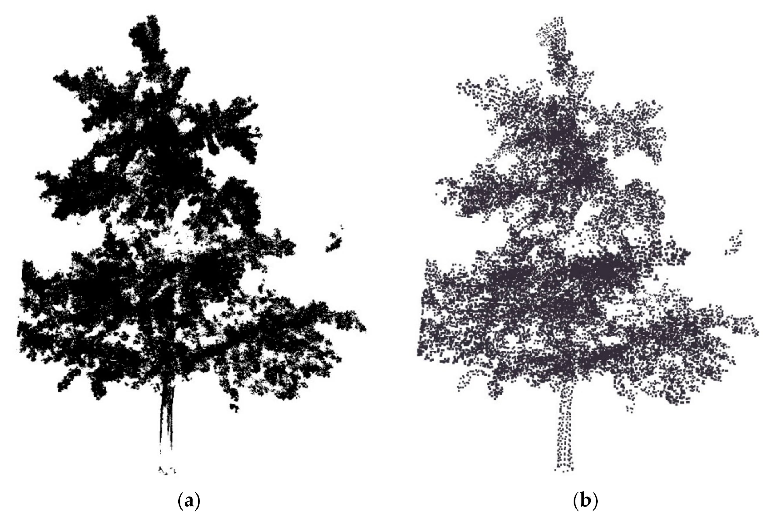
In this paper, two sets of point clouds obtained from TLS for two ginkgo trees in different seasons were used for this experiment. Both of two trees were in the campus of University of Tennessee, Knoxville, USA. One of them was obtained when one ginkgo tree had leaves, while the other was acquired when the leaves of another tree fell off. Those rough data were processed with error calibration, registration, noise removal, and region segmentation to derive the original tree point clouds shown in Figure 1a,b. The numbers of the point clouds were 1,974,535 and 348,868, with the 3D extent X (8.4 m) × Y (8.33 m) × Z (10.85 m) and X (8.28 m) × Y (7.1 m) × Z (14.37 m), and the average distance 0.06 m and 0.05 m, respectively. Due to the self-shelter of the tree, there were several hiatuses of the trunk in Data 1, as presented in Figure 1a.

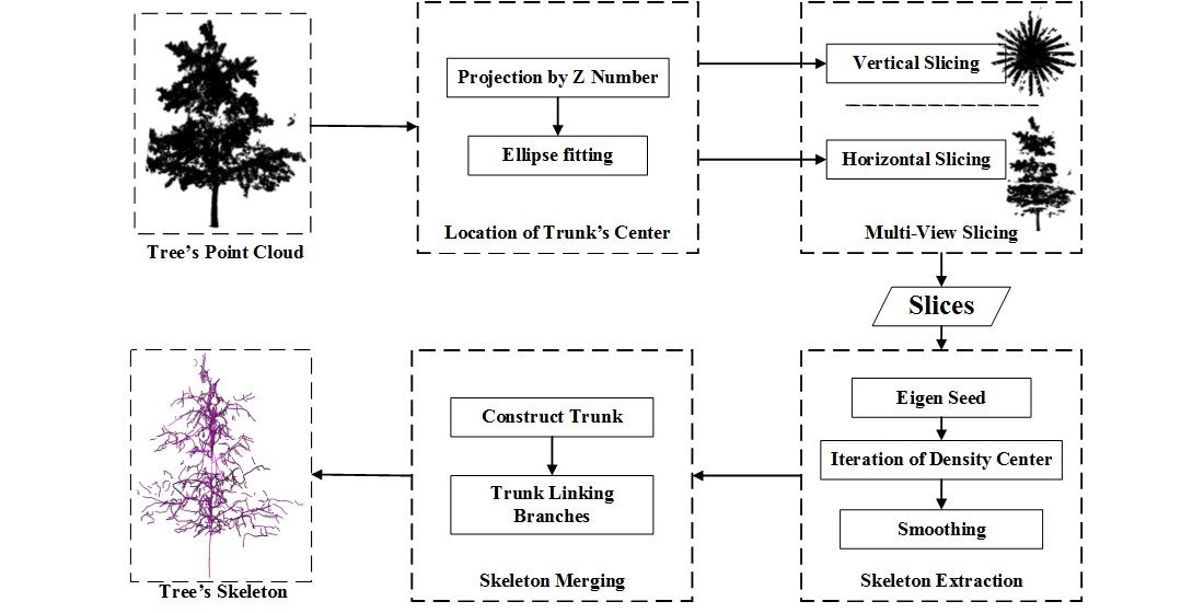
The framework was inspired by X-ray computed tomography (CT) [31] so that the building tree skeleton model was based on slices from multiple views. Therefore, a divide and conquer—merge strategy was adopted in this paper, as shown in Figure 2.

According to this inspiration, all the procedures focused on slicing, including locating the precise center of tree trunk, extracting, and merging skeletons from slicing parts of point cloud. There were two types of slicing, namely vertical slicing and horizontal slicing. The horizontal slicing was almost similar to the method of CT, while the vertical slicing cuts the tree’s point clouds into pieces like the petals of the flower. The center of the tree trunk was obtained by ellipse fitting on the projection image along the Z axis. These slices of point clouds were the input for the proposed skeleton extraction algorithms. Therefore, this step was performed under the assumption that the up direction of the acquired point clouds was along the Z axis. In the following steps, the separate skeleton segments generated from these slices were linked and merged to form the final tree skeleton model. The following part in this section describes the details of these procedures.

2.1. Location of the Tree Trunk’s Center

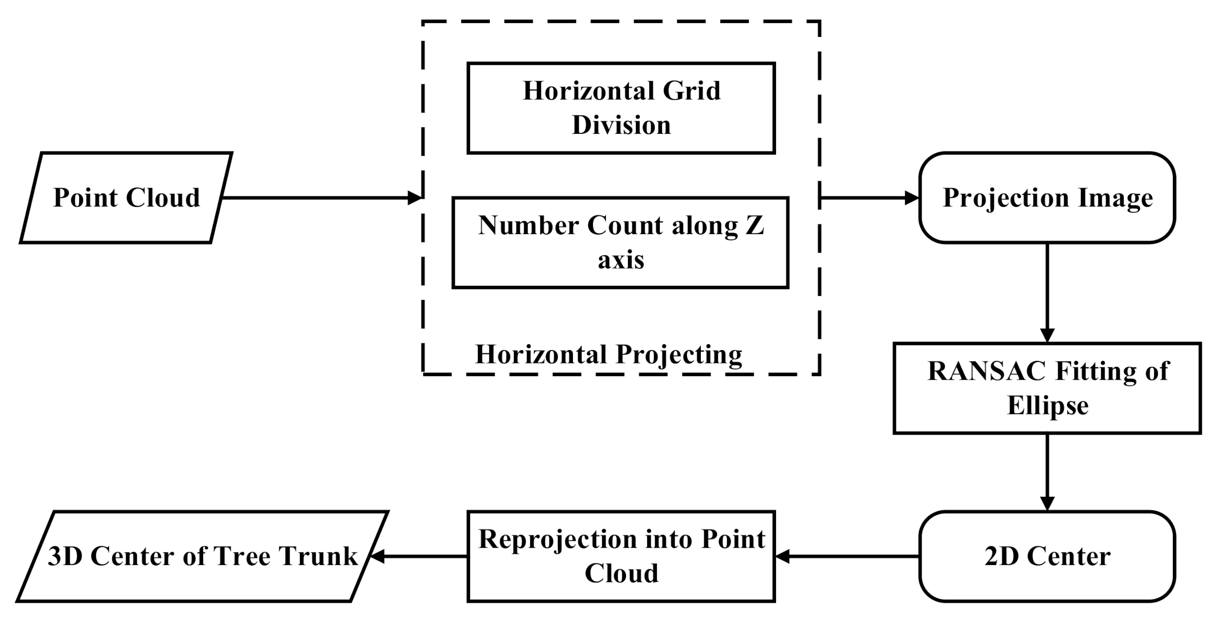
The ecological structure of trees indicates that the basic elements (e.g., roots, trunks, limbs, branches, and leaves) compose a tree. Among these elements, the trunk is the basepoint of the aboveground parts of the tree. Some methods directly use the lowest point as the root or the start of trunk [17,18,32,33,34]. Similarly, in this paper, we first located the precise center of the trunk before slicing, the workflow of which is given in Figure 3.

The point cloud from TLS represents the surface of the object in the form of discrete points so that less occlusion can increase the density of the point cloud with the same or similar reflection. According to this property, the tree trunk was obvious in the point cloud with a large amount of high-reflection points. It was coincident with the structure of tree model in nature. Therefore, the center of tree trunk could be the reference for slicing. Thus, we first extracted the center of the tree trunk by projecting the point cloud to a 2D image in this approach, and then detecting the ellipse by using the random sample consensus (RANSAC)-based method [35]. It is worth noting that the resolutions of the projected image along the X,Y axes, which were set according to the density of the tree’s point cloud, were the same to avoid deformation. The detection of the ellipse on the projected image could not give the 3D coordinate; thus, the fit circle was then re-projected into the point cloud to search neighbor points for calculating precise center. This projection along the Z axis is irreversible so that the rich three-dimensional discrete point information contained in the single point cloud would be lost. Therefore, the re-projection would be difficult in some direct way. An effective method connecting the circle center on the projection image with the corresponding 3D position was to traverse the point cloud for those points which were used for fitting the 3D coordinates of the circle center. The details of locating the tree trunk’s center are described as follows:

Step 1: Project the point cloud along the Z axis into XOY plane with the number of points, and transform the projection grids of the numbers of point cloud into the image;

Step 2: Search and fit the ellipse with RANSAC on the image;

Step 3: Traverse all the point cloud and find those points whose XY are in accordance with the fitted ellipse;

Step 4: Fit the planar ellipse again with these consistent points’ XY coordinates, and set the ellipse’s elevation to the minimum of the point cloud.

2.2. Slicing

It is well known that the tremendous amount of point clouds is a computation and memory bottleneck for 3D tree modeling. Slicing may deal with this issue to some degree by efficiently decreasing the amount of point cloud in one go. In this paper, there is an anchor for slicing, which is the center of tree trunk captured in the previous section. Two forms of slicing were introduced in this paper: Vertical slicing and horizontal slicing. Horizontal slicing is much easier to complete, as it just divides the point cloud into slices with several height intervals. In our experiments, two manners of horizontal slicing, namely 5-equidistant and 10-equidistant division of horizontal slicing, were used.

The left part (a) in Figure 4 shows one instance of horizontal slicing, 10-equidistant division, from the front view. The right part (c) in Figure 4 reveals the essence of vertical slicing from the top view that the axis is from the center of tree trunk along the direction of positive elevation. In the manner of vertical slicing, the point cloud was equally divided into slices with an interval of $\theta$ degree, as shown in the middle and right parts of Figure 4. The intervals with a width separated the points. In this paper, the $\theta$ was obtained through the number of slices, namely $\theta =180/n$. $n$. ranged from 2 to positive infinity. As can be seen from Figure 4b,c, there would be much loss of points when $n$. is 2, while there would be many small slices of points when $n$ became much bigger. In our experiment, $n$ was empirically chosen from the set [4,8,12], e.g., 8 in Figure 4c.

The details are designed as follows:

(1)

Prepare the coordinates of the tree’s trunk center $O$ and the interval width equivalent to the short semi-axis of the detected ellipse from the previous description, and set the number of slices $n$, default is 8. In our experiments, the value of $n$ was set to 4 and 8, or another positive integer. Then the interval angle $\theta$ is obtained;

(2)

Calculate the interval lines’ parameters, for instance the red and blue dash lines, as $y=kx+c$ based on the center $O$ according Figure 4b;

(3)

Determine in which slice the points are, whether their horizontal distance to the interval lines is less than the width.

It is worth noting that all the slices shared the points near the center, which is clearly presented in Figure 4c, and is useful in the merging step in the following Section 2.3.

2.3. Skeleton Extraction and Merging

The skeleton extraction began with the seed points generated by adaptive scale method. Then all of the skeletons were extracted from the sliced point cloud by using kernel mean shift (KM-S) and kernel principal component analysis (KPCA). Furthermore, the proposed method adopted a growing strategy algorithm to merge all the skeletons to generate the whole 3D tree skeleton model. The flowchart in Figure 5 outlines the primary steps of skeleton extraction and merging.

2.3.1. Seed Points Extraction

In this section, we propose an adaptive scale method to generate the initial seed set inspired by dimensionality features [36,37]. The 3D dimensionality feature was more likely to distinguish tree trunk/branches and leaves. However, it was difficult to define the scale for calculating dimensionality features. The solution in this paper was to model the pattern of trees, as it is well known that the tree is always like a horn-shaped bell. We defined the maximum scale as the semi-major axis obtained in Section 2.1, and the minimum scale as the average distance of original point cloud. Then the maximum scale of each point was calculated according to its height and horizontal distance to the tree center. The average distance made a distinction between different scales. The dimensionality features of each point would be processed in several scales. A point was selected as a candidate only if its 3D dimensionality feature was larger than other features in any scale.

The candidate seeds were still far too many, as a large number of points on the tree trunk and branches were candidate points. Then a hybrid voxel filter was under operation on the candidate seeds. The voxel size was the average of the maximum and minimum scale. The voxel filter picked a point from the seed candidates if there were candidates in the voxel, or from the original point cloud if there were not. Figure 6 shows the seed candidates and the final seeds of the tree point cloud in Figure 1a. There were only 22,603 points in the final seed point cloud, while the number was 1,640,632 in the candidate point cloud.

2.3.2. Kernel Mean Shift Algorithm (KM-S)

The mean shift algorithm is a type of nonparametric kernel density estimation [38]. The kernel function estimation method can asymptotically converge to any density function in the case of sufficient sampling. Therefore, mean shift can be used to estimate density for any data subject to any distribution.

Given $n$ samples in d-dimensional space $R^d x_i$, $i=1,2,\dots ,n$, the mean shift vector $M_r\left(x\right)$ of $x$ is written as follows:

$$M_r\left(x\right)=\frac{1}{k}{{\displaystyle \sum }}_{x_i\in S_r}\left(x_i-x\right)$$

(1)

where $k$ is the number of points which is within the sphere neighborhood ${\mathrm{S}}_r$ of $x$ with the radius $r$. That is:

$$S_r\left(x\right)=\left\{y:{\left(y-x\right)}^T\left(y-x\right)\le r^2\right\}$$

(2)

After adding a kernel, the mean shift changed to be:

$$f_{r,K}\left(x\right)=\frac{c_{k,d}}{n{r}^d}{\displaystyle \sum }_{i=1}^{n}k({\Vert \frac{x-x_i}{r}\Vert }^2)$$

(3)

where $\frac{c_{k,d}}{n{r}^d}$ is the unit density, and both $K$ and $k$ represent the kernel. The gradient of Equation (3) is

$$\nabla f_{r,K}\left(x\right)=\frac{2c_{k,d}}{n{r}^{d+2}}{\displaystyle \sum }_{i=1}^n\left(x-x_i\right)k^{\prime }({\Vert \frac{x-x_i}{r}\Vert }^2).$$

(4)

Then, we introduced a new kernel:

$$g\left(x\right)=-k^{\prime }\left(x\right)$$

(5)

aowing $g\left(x\right)$ into Equation (4) yielded:

$$\begin{gathered} \nabla f_{r,K}\left(x\right)=\frac{2c_{k,d}}{n{r}^{d+2}}{\displaystyle \sum }_{i=1}^n\left(x_i-x\right)g\left({\Vert \frac{x-x_i}{r}\Vert }^2\right)\nabla f_{r,K}\left(x\right) \\ \nabla f_{r,K}\left(x\right)=\frac{2c_{k,d}}{n{r}^{d+2}}\left[{\displaystyle \sum }_{i=1}^{n}g\left({\Vert \frac{x-x_i}{r}\Vert }^2\right)\right]\left[\frac{{{\displaystyle \sum }}_{i=1}^n{x}_{i}g\left({\Vert \frac{x-x_i}{r}\Vert }^2\right)}{{{\displaystyle \sum }}_{i=1}^{n}g\left({\Vert \frac{x-x_i}{r}\Vert }^2\right)}-x\right] \end{gathered}$$

(6)

The second term in Equation (6) is the mean shift:

$$m_{r,G}\left(x\right)=\frac{{{\displaystyle \sum }}_{i=1}^n{x}_{i}g\left({\Vert \frac{x-x_i}{r}\Vert }^2\right)}{{{\displaystyle \sum }}_{i=1}^{n}g\left({\Vert \frac{x-x_i}{r}\Vert }^2\right)}-x$$

(7)

This shift demonstrated the difference between the original center $x$ and the new mean $\frac{{{\displaystyle \sum }}_{i=1}^n{x}_{i}g\left({\Vert \frac{x-x_i}{r}\Vert }^2\right)}{{{\displaystyle \sum }}_{i=1}^{n}g\left({\Vert \frac{x-x_i}{r}\Vert }^2\right)}$.

2.3.3. Kernel Principal Component Analysis (KPCA)

Mean shift is always recursive for local maxima leading to too-close cluster centers to classify them. In other words, the mean shift algorithm further contracts to the global density center after obtaining the local center. Thus, there should be some additional constraints in mean shift. In this paper, we adopted kernel principal component analysis (KPCA) [39] to solve this problem. KPCA is a nonlinear extension of PCA using techniques of kernel methods. KPCA overcomes the difficulty of linearly inseparable classification in PCA. The kernel extension of PCA further matches well with mean shift for algorithm designing and implementing.

Given a set of $n$ observations in d-dimensional space $R^d x_i$, $i=1,2,\dots ,n$, PCA sets the covariance matrix:

$$C=\frac{1}{n}{\displaystyle \sum }_{i=1}^n\left(x_i-x_0\right){\left(x_i-x_0\right)}^T$$

(8)

where $x_0$ is the center of the set of $n$ observations.

Using a kernel function, the covariance matrix can be written as a new equation:

$$\overline{C}=\frac{1}{n}{\displaystyle \sum }_{i=1}^{n}K\left(x_i-x_0\right)K{\left(x_i-x_0\right)}^T$$

(9)

The mapping of observations onto the eigenvectors of the covariance matrix can be calculated for extracting the principal components as follows:

$$pz={{\displaystyle \sum }}_{i=1}^n{\mathsf{\alpha }}_i^{k}K\left(x_i-x_0\right)$$

(10)

Let ${\mathsf{\lambda }}^1\le {\mathsf{\lambda }}^2\le \dots \le {\mathsf{\lambda }}^n$ denote the eigenvalues, and ${\mathsf{\alpha }}^1,\dots ,{\mathsf{\alpha }}^n$ the corresponding complete set of eigenvectors. For one sample $x_i$ in 3D space around with the m-neighbors, the local surface smoothness can be calculated by:

$${\mathsf{\sigma }}_{x_i}= \frac{{\lambda }_2}{{\lambda }_0+{\lambda }_1+{\lambda }_2}$$

(11)

To avert too-close cluster centers, the following equation was constructed in accordance with the mean shift:

$$f_{r,K}\left(x\right)=\frac{c_{k,d}}{n{r}^d}{\displaystyle \sum }_{o\in O}K(\Vert \frac{x-x_i}{r}\Vert )+{\displaystyle \sum }_{d\in D}\frac{\mathit{K}\left(\Vert x-x_d\Vert \right)}{{\sigma }_i\Vert x-x_d\Vert }$$

(12)

where $O$ is the set of the original point cloud and $D$ is the set of density centers.

The modes of the density function are located at the zeros of the gradient function $\nabla f_{r,K}\left(x\right)=0$. The gradient of the density estimator is:

$$\nabla f_{r,K}\left(x\right)=\frac{c_{k,d}}{n{r}^{d+2}}{{\displaystyle \sum }}_{o\in O}\left(x-x_o\right)k^{\prime }\left(\Vert \frac{x-x_i}{r}\Vert \right)-2{\displaystyle \sum }_{d\in D}\frac{\left(x-x_d\right)k^{\prime }\left(\Vert x-x_d\Vert \right)}{{\sigma }_i\Vert x-x_d\Vert {}^2}=0$$

(13)

Setting $\mathsf{\mu }=\frac{{{\displaystyle \sum }}_{d\in D}\frac{k^{\prime }\left(\Vert x-x_d\Vert \right)}{\Vert x-x_d\Vert {}^2}}{{\sigma }_i{{\displaystyle \sum }}_{o\in O}{k}^{\prime }\left(\Vert \frac{x-x_i}{r}\Vert \right)}$, we rearranged Equation (13) to be:

$$\left(1-\mathsf{\mu }{\sigma }_i\right)x+\mathsf{\mu }{\sigma }_i\frac{{{\displaystyle \sum }}_{d\in D}{x}_d\frac{k^{\prime }\left(\Vert x-x_d\Vert \right)}{\Vert x-x_d\Vert {}^2}}{{{\displaystyle \sum }}_{d\in D}\frac{k^{\prime }\left(\Vert x-x_d\Vert \right)}{\Vert x-x_d\Vert {}^2}}=\frac{{{\displaystyle \sum }}_{o\in O}{x}_o{k}^{\prime }(\Vert \frac{x-x_i}{r}\Vert )}{{{\displaystyle \sum }}_{o\in O}{k}^{\prime }(\Vert \frac{x-x_i}{r}\Vert )}$$

(14)

Equation (14) can be considered as a set of equations with X as unknowns, which can be used to get the relationship between the next iteration and current iteration as Equation (15):

$$x_{i+1}=\frac{{{\displaystyle \sum }}_{o\in O}{x}_o{k}^{\prime }(\Vert \frac{x-x_i}{r}\Vert )}{{{\displaystyle \sum }}_{o\in O}{k}^{\prime }(\Vert \frac{x-x_i}{r}\Vert )}+\mathsf{\mu }{\sigma }_i\frac{{{\displaystyle \sum }}_{d\in D}\left(x_i-x_d\right)\frac{k^{\prime }\left(\Vert x-x_d\Vert \right)}{\Vert x-x_d\Vert {}^2}}{{{\displaystyle \sum }}_{d\in D}\frac{k^{\prime }\left(\Vert x-x_d\Vert \right)}{\Vert x-x_d\Vert {}^2}}$$

(15)

2.3.4. Details of Skeleton Extraction

The presented skeleton extraction algorithm started from several initial density centers, as described in the kernel mixture of mean shift and PCA. The skeleton model was generated by iterative computation from the initial density center. The number of density centers would affect the fine skeleton and computation time. Generally speaking, more density centers promote the fine skeleton, while increasing the computation time and memory. There should be a trade-off in practice. This paper used the extracted seed points as initial density centers.

The iterative procedure was designed for the point cloud to be contracted to local density centers, and the iteration was to avoid these local density centers contracting to global density centers. Then, these local centers were well arranged along the tree trunk and limbs or branches to form the skeleton model. This iterative scheme was similar to that used in the state-of-the-art methods [27].

In our KM-S and PCA algorithm, the iteration involved two kinds of set, $O$ and $D$. The initial $S_{ori}$, the neighbor points of the local density center, depended on the neighbor radius $r$ and the spatial location of the corresponding local center $x_d$ in $D$. On the other hand, KPCA constrained the distances between local density centers. The two main sets were intertwined so that they could not be solved in one iteration. We adopted an alternating iteration algorithm that effectively decoupled the variable updates. The basic idea was to alternate between the iterating radius and iterating density centers.

The details of the alternating iteration are described as follows:

(1)

The seeds are selected in the input sequence of the original point cloud $O$ as initial local density centers to constitute $D$ following the algorithm in Section 2.3.1;

(2)

Given the searching radius $r$, collect the neighbors of local density centers in $D$ as $S_{den}$, and calculate ${\mathsf{\sigma }}_i$ for every density center with Equation (11);

(3)

Similarly, get the neighbors of local density centers in $O$ as $S_{ori}$ with $r$.

(4)

For every local density center $x_i$ in $D$, calculate ${\mathrm{v}}_{pca}=\frac{{{\displaystyle \sum }}_{d\in D}\left(x_i-x_d\right)\frac{k^{\prime }\left(\Vert x-x_d\Vert \right)}{\Vert x-x_d\Vert {}^2}}{{{\displaystyle \sum }}_{d\in D}\frac{k^{\prime }\left(\Vert x-x_d\Vert \right)}{\Vert x-x_d\Vert {}^2}}$ with neighbors in: $S_{den}$, ${\mathrm{v}}_{ms}=\frac{{{\displaystyle \sum }}_{o\in O}{x}_o{k}^{\prime }(\Vert \frac{x-x_i}{r}\Vert )}{{{\displaystyle \sum }}_{o\in O}{k}^{\prime }(\Vert \frac{x-x_i}{r}\Vert )}$ with neighbors in $S_{ori}$;

(5)

Obtain the new center $x_{i+1}$ with Equation (15);

(6)

If the times of iterations are less than the threshold (100 in this paper), or the change of center is larger than another threshold (0.0001 in this paper), turn to (2) with the radius fixed;

(7)

Then gradually increase the radius. Go to (2) for next iteration.

In our experiment, $r$ was initialized and increased adaptively with the size of original point cloud, the same as in [7,27]. The iteration stopped when all seeds were processed, or the times reached 100. Despite all these iterations, the discrete skeleton points generated by the mixed algorithm with KM-S and KPCA were not in accordance with the pattern of normal growth of natural trees. Soon afterwards these points were smoothed on each skeleton with the Douglas–Peucker method [40].

2.3.5. Skeleton Merging

This section describes the merging part of the divide and conquer—merge strategy, after the skeletons of each slice have been extracted by the KM-S and KPCA methods. The division operation earned the advantage of easy computation, but brought on side effects including that vertical slicing led to multiple skeletons in the central areas, and horizontal slicing resulted in a fractured central skeleton. The designed merging algorithm dealt with this problem. The algorithm incrementally merged and linked adjacent skeleton vertexes with a similar direction into a set of skeletons:

(1) Collect the skeleton vertexes near the tree center from horizontal perspective to create a new skeleton. The horizontal distance threshold is the linear correlation with the height of the skeleton vertex according to the pattern of trees, as described in the same model in Section 2.3.1. The XYZ coordinates of these vertexes are respectively averaged to obtain the new skeleton every average distance of original point cloud. Add this new skeleton to the extracted skeleton set;

(2) Estimate an ellipse for each skeleton vertex with its neighbor points. We define a plane that passes through the vertex and has a normal ellipse along with the direction of the branch at the location of this skeleton vertex. The neighbor points are not only near the vertex, but the plane. These neighbor points are projected on the plane for further being used to estimate the ellipse with RANSAC, the same way as in Section 2.1. The parameters of the ellipse during the random iterations are computed with the direct fitting method [41]. The radius or area of ellipse is just used for sorting the order of vertex in the following steps, but not for fine-tuning the location of the curve skeleton, since there are missing neighbor points;

(3) Ensure the vertexes of each skeleton in the order of continuous consistency of the ellipse radius or area, rather than singe ellipse radius or area. Here, continuous consistency of the ellipse radius or area means that the head should be thicker than the tail in one skeleton, which makes the sorting more moderate;

(4) Incrementally merge to form the trunk skeleton. The iteration begins with the lowest pair of skeleton vertexes. Find the vertexes in the cone that the pair into a temporary set. Create a candidate set with the vertexes not in the cone from the skeletons that the vertexes of the temporary set belong to. There is only one vertex for one element in the temporary set, and the vertexes in the candidate set are the nearest ones not in the cone along with the direction of their skeleton. Soon afterwards, select the one from the candidate set as the next vertex of the trunk skeleton if the direction between the line from it to the top vertex and the new cone is smallest, and if the continuous consistency of the skeleton that it belongs to is largest. This rule makes sure that the trunk is the thickest and smoothest. Remove the candidate if it is not in the new cone that the top pair of vertexes of the trunk skeleton constitutes. Continue this iteration until there are no more candidates. Then, extend the trunk skeleton to an upper vertex so that the distance to top vertex of trunk is less than 2 times of the height of the newest cone. If there are several vertexes meeting the distance requirement, pick the one with the largest continuous consistency of ellipse radius. This increase-extend proceeds alternately until there is no more vertex that could be processed. Therefore, the skeleton of trunk is obtained. During the alternation procedure, the skeletons, the parts of the vertexes of which are in the cones formed by the trunk skeleton, are skeletons. Those skeletons, all of which are in the cones, are deleted. This semantic rule could be further applied to identify and label the twigs;

(5) Link the unlabeled skeleton to the labeled skeletons if the nearest distance from any vertex in the unlabeled skeleton to a labeled skeleton is smaller than the same threshold in the presented operation of extension. These skeletons that just connected are labeled according to the types of the skeletons being connected.

When all of the procedures were completed, the skeletons of a tree could be generated from the original point cloud. The designed method also obtained the semantic information about the skeleton.

3. Results and Discussion

This section firstly shows the visual effect of our algorithm based on two datasets of point cloud. Afterwards, some discussions including the method of slicing and comparison with the state-of-the-art methods are presented. The limitations are illustrated at the end of this section.

3.1. Visual Effect of Results

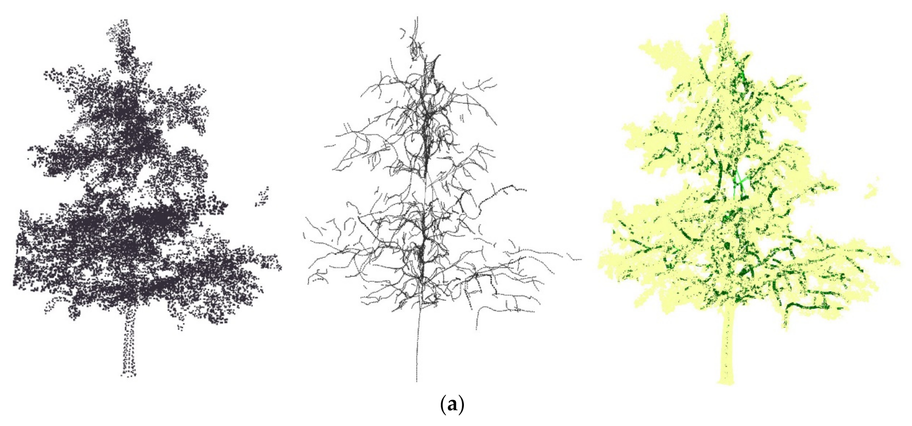
The skeletons of two ginkgo trees in different seasons and structure were obtained, as shown in Figure 7. Direct visual observation could tell that Data 1 had more branches than did Data 2. Our method generated skeletons of the main structure for both datasets. The results of these two trees demonstrated that our algorithm was able to deal with different shapes and structures, and that the skeletons were basically not affected by the leaves. It could be observed that seed extraction, skeleton calculation and the merging strategy contributed to the results. The seed points were evenly distributed. Slicing was conducive to produce more skeletons, and merging helped to maintain the structure of trees. The method of slicing is discussed in the following part.

3.2. Discussion on the Method of Slicing

The key parameter in our method was the method of slicing. There are many methods of slicing on point clouds, such as the horizontal or vertical equiangular or equidistant methods, for example, “⌗” or “✴”. The extraction result is affected by the manner of slicing. In this paper, we chose vertical equiangular and horizontal equidistant slicing in accordance with the natural structure of the trees. Horizontal slicing divided the experiment data into five and ten equal parts. The number of intervals could be adapted according to the tree species or depending on the environmental conditions, so it is out of this paper. We chose two manners of horizontal slicing, namely 5-equidistant and 10-equidistant division of horizontal slicing. In the meantime, the 4-equiangular, 8-equiangular, and 12-equiangular division of vertical slicing were used for experiment and comparison.

In order to view and compare the results, we put the side view of slicing, the extracted and merged skeletons in the same table, as presented in

Table 1. The results of our methods on two datasets in two different seasons. The methods of slicing are presented in the first column in the form of abbreviation, such as V-4 short for the 4-equiangular division of vertical slicing and H-5 short for 5-equidistant division of horizontal slicing. The slicing columns of Data 1 and Data 2 show the side views of sliced point clouds. The vertical slicing shows the top view, and the horizontal slicing presents the front view with several virtual intervals. The columns of “Extracted Skeletons” exhibit the skeletons generated from the pieces of sliced point clouds. The columns of “Merged Skeletons” demonstrate the final results of our methods.

	Data 1			Data 2
	Slicing	Extracted Skeletons	Merged Skeletons	Slicing	Extracted Skeletons	Merged Skeletons
(a) V-4
(b) V-8
(c) V-12
(d) H-5
(e) H-10

. Both of the two manners of slicing produced relatively complete skeletons of tree trunk. The designed vertical slicing benefitted several skeletons in the trunk area (rows a–c in Table 1), and the horizontal slicing benefitted the coherence of horizontal branches (rows d–e in Table 1). On the contrary, the vertical slicing lost the point cloud when cutting, and the horizontal slicing broke the central skeletons when extracting. Hence, the higher the number of vertical slices, the higher the number of branches (rows a–c in Table 1). Similar side effects were shown in horizontal slicing, i.e., that the higher the number of horizontal slices, the more breaks there were. Obviously in this experiment, vertical slicing kept the point data to a maximum extent in every piece so that every piece contained the points of the tree trunk. This method of slicing obtained more information on the central skeleton. However, the horizontal slicing made the original point cloud artificially divide into equal parts in the manner of equal height. Despite keeping much more branch and limb skeletons as indicated in rows d and e, horizontal slicing separated the natural growth structure of the tree into segments, inciting the scattered branch skeletons if the scanning point data was missing or occluded. It is easy for horizontal slicing to cause fragmentation in the central skeleton of tree trunk.

In spite of these problems, our designed merging strategy was destinated to settle the difficulties, which can be seen in the column of merged skeletons in Table 1. All of these merged skeletons remained as one central skeleton of the tree trunk, as we merged several skeletons from vertical slicing and linked the fractured parts from horizontal slicing. It is obvious in rows a–c of Data 1 that the breaks in the trunk area were connected and the skeleton was smooth along the direction of the trunk. This advantage was also shown in other result figures, especially in the lower trunk of the tree. However, the curved shape of the tree and incompleteness of the point cloud in Data 1 and Data 2 held up the increase of the merging algorithm in the upper trunk. Calculated with the original point cloud, the radiuses and directions of the skeleton vertexes could not keep further growing of the merging algorithm in the upper trunk.

In general, the proposed divide and conquer—merge strategy could overcome the problem that there were breaks in the trunk area and obtain the comparatively complete skeleton models of two different datasets. The vertical slicing kept the central part of the point cloud and skeletons, and the merging algorithm succeeded in dealing with several central skeletons of the tree trunk. The merging algorithm also connected the artificial breaks introduced by horizontal slicing. The vertical slicing performed better than the horizontal slicing from a holistic perspective.

3.3. Comparison with State-of-the-Art Methods

The tree’s botanical structure could be expressed in the form of the skeleton and other manners, such as volume model. Therefore, a comparison on botanical structure with three state-of-the-art methods, SimpleTree [18], PypeTree [17], and L1-Skeleton [27] was performed. L1-Skeleton, SimpleTree, and our method have been compiled on Win64 bits operation system with Visual C++. In the meantime, it should be illustrated that PypeTree could not process point cloud data with a large number of points, due to the Win32 runtime environment and complex compatibility of several dependent libraries. During the comparison, the number of points in Data 1 and Data 2 were respectively reduced to 138,793 and 90,388, with the voxel grid filtering just for PypeTree, while the proposed method, SimpleTree, and L1-Skeleton processed the original point cloud of Data 1 and Data 2.

Table 2. Comparison on maximum memory, run time, and number of skeletons of different methods.

	Our Method (V-12)			SimpleTree			PypeTree			L1
	Max Mem	Time (m)	Number	Max Mem	Time (m)	Number	Max Mem	Time (m)	Number	Max Mem	Time (m)	Number
Data1	3.4G	33	808	0.99G	3	350	1.20G	34	354	12.6G	77	49
Data2	1.6G	18	637	0.44G	2	495	0.95G	26	573	3.2G	20	249

displays the statistically counted results of maximum memory, run time, and the number of skeletons. Since these algorithms were implemented in different ways and by different persons, it is unfair to compare the run time and memory directly. Thus, the run time and maximum memory in Table 2 are just for reference. It is noted that the numbers of skeletons obtained by SimpleTree and PypeTree in Table 2 actually counted the cylinders, which meant that two points constituted one skeleton. On the contrary, the skeleton generated by L1-Skeleton and our method was mostly composed of several points. In spite of this, our method still yielded the maximum number of skeletons.

In respect to the visual examination based on observing the constructed graphs, the results of the state-of-the-art methods processing Data 1 and Data 2 are shown in Figure 8. The results of Data 1 obtained by three methods were far less than those of our method, no matter which the way of slicing was, though Figure 8a,b presents that SimpleTree and PypeTree succeeded in the lower part of the trunk. Figure 8c illustrates that L1-Skeleton failed to calculate the structure of the tree on Data 1. The better results in Figure 8d–f indicated that the point cloud like Data 2 was easy for these methods to process. The skeleton of trunk was marked and continual in the result of SimpleTree in Figure 8d, which was similar to that of the proposed method. In the meantime, the skeleton of the trunk was less marked and discrete in the results of PypeTree and L1-Skeleton in Figure 8e,f. Furthermore, the number and completeness of branches and limbs of the results calculated by the state-of-the-art methods on Data 2 were also less compared to those derived from the presented method.

From this comparison, it could be generally concluded that the proposed framework was more effective than the state-of-the-art methods, namely SimpleTree, PypeTree, and L1-Skeleton. It was difficult for SimpleTree or PypeTree to connect the sphere or level set neighbors produced from the serious self-occluded point cloud, which led to their gloomy results of the skeleton. Instead of using the continuity of element neighbors, L1-Skeleton could be considered as a regularized mean shift that can generate skeletal points, which is similar to our KM-S methods. Benefiting from the divide and conquer—merge strategy, seed selection, and KPCA, our methods generated more skeleton of the branches and complete trunk skeletons than L1-Skeleton.

3.4. Limitations

Our proposed framework obtained relatively complete tree skeletons from the point cloud, and the comparative evaluation demonstrated the effectiveness and advantage over state-of-the-art methods. In general, the divide and conquer strategy of multi-view slicing framework was capable of avoiding a large demand of computer memory to extract tree skeletons from a large amount of point cloud data. The merge strategy dealt with the difficulty introduced by the division operation. However, there were still existing some limitations within our proposed method.

Firstly, as this method was designed for common trees with vertical patterns like the two trees in the experiment, its extent of application is constrained, such as when considering crooked trees. As for the center location of the tree trunk, the projection was the dimension reduction operation, which was implicitly based on the prerequisite that the trunk of tree could not be too bent. If so, the pixels projected on the 2D plane were so scattered that it would not form a circle for ellipse fitting. In this case, the vertical slicing may fail to continue. It should be noted that this will not be an obstacle for horizontal slicing.

Secondly, vertical slicing kept the more vertical structures of trees, for instance, the tree trunk, than horizontal slicing. In general, horizontal slicing cut through the vertical structures of trees, leading to breaks in the skeleton extraction stage. It made a block for the following merging and linking. That is why we did not carry out more experiments on horizontal slicing, such as the intervals which are naturally related to the species of tree.

Thirdly, there were isolated skeletons in our results which were not connected to the trunk, other branches, or twigs. The directions along most of these insular skeletons were not near those of neighbor skeletons. Therefore, our method was seldom able to link them directly. Furthermore, there were wrong links which should be further improved.

At last, since the point cloud of trees was the input of our framework approach, the effect of the input data defect was similar to other algorithms [7,16,27]. Therefore, severe occlusion and large missing data imposed the limitations and gaps on our methods.

4. Conclusions

In this paper, we proposed an effective multi-view slicing-based framework for tree modeling from point clouds. In this framework, the center of the tree trunk was the first to be extracted by projecting the multi-view point clouds obtained from TLS to the horizontal plane before slicing. Inspired by the medical CT technique, the point cloud was sliced into pieces in a vertical and horizontal manner. The skeleton was extracted from every slice with a novel kernel mixture of mean shift and PCA. Then, these skeletons of the tree trunk, limbs, and branches were merged by simply merging and linking. Experiments on slicing illustrated that both vertical and horizontal slicing produced most skeletons of the tree trunk, limbs, and branches, and that vertical and horizontal slicing gained its own performance. Comparative evaluations on two ginkgo trees in different shapes and patterns, with and without leaves, indicated that our constructed tree skeletons could correctly capture more skeletons and links among branches under an acceptable reconstruction completeness.

For future application of this proposed model, there is much more work to improve and optimize this framework. The initial density centers of the kernel mean shift algorithm could be selected by designed sampling methods in accordance with the properties of trees besides adaptive scale sampling. The method of slicing could be optimized to apply to tilt and over-curved trees, as well. The above directions should be taken into consideration by improving our proposed model in this preliminary work.

References

- Sheppard, J.P.; Morhart, C.; Hackenberg, J.; Spiecker, H. Terrestrial laser scanning as a tool for assessing tree growth. iForest Biogeosci. For. 2017, 10, 172–179. [Google Scholar] [CrossRef]
- Liang, X.; Kankare, V.; Hyyppä, J.; Wang, Y.; Kukko, A.; Haggrén, H.; Yu, X.; Kaartinen, H.; Jaakkola, A.; Guan, F.; et al. Terrestrial laser scanning in forest inventories. ISPRS J. Photogramm. Remote Sens. 2016, 115, 63–77. [Google Scholar] [CrossRef]
- Stovall, A.E.L.; Vorster, A.G.; Anderson, R.; Evangelista, P.H.; Shugart, H. Non-destructive aboveground biomass estimation of coniferous trees using terrestrial LiDAR. Remote Sens. Environ. 2017, 200, 31–34. [Google Scholar] [CrossRef]
- Huang, H.; Tang, L.; Chen, C. A 3D individual tree modeling technique based on terrestrial LiDAR point cloud data. In Proceedings of the 2015 2nd IEEE International Conference on Spatial Data Mining and Geographical Knowledge Services (ICSDM), Fuzhou, China, 8–10 July 2015. [Google Scholar]
- Lau, A.; Bentley, L.P.; Martius, C.; Shenkin, A.; Bartholomeus, H.; Raumonen, P.; Malhi, Y.; Jackson, T.; Herold, M. Quantifying branch architecture of tropical trees using terrestrial LiDAR and 3D modelling. Trees-Struct. Funct. 2018, 32, 1219–1231. [Google Scholar] [CrossRef] [Green Version]
- Liang, X.; Hyyppä, J.; Kaartinen, H.; Lehtomäki, M.; Pyörälä, J.; Pfeifer, N.; Holopainen, M.; Brolly, G.; Francesco, P.; Trochta, J.; et al. International benchmarking of terrestrial laser scanning approaches for forest inventories. ISPRS J. Photogramm. Remote Sens. 2018, 144, 137–179. [Google Scholar] [CrossRef]
- Mei, J.; Zhang, L.; Wu, S.; Wang, Z. 3D tree modeling from incomplete point clouds via optimization and L1-MST. Int. J. Geogr. Inf. Sci. 2017, 31, 999–1021. [Google Scholar] [CrossRef]
- Chen, X.; Neubert, B.; Xu, Y.Q.; Deussen, O.; Kang, S.B. Sketch-based tree modeling using Markov random field. In Proceedings of the Special Interest Group on Computer Graphics and Interactive Techniques Conference (ACM. SIGGRAPH ’08), Singapore, 10–13 December 2008; Volume 27. [Google Scholar]
- Rutzinger, M.; Pratihast, A.K.; Oude Elberink, S.; Vosselman, G. Detection and modelling of 3D trees from mobile laser scanning data. Int. Arch. Photogramm. Remote Sens. Spat. Inf. Sci. 2010, 38, 520–525. [Google Scholar]
- Tagliasacchi, A.; Delame, T.; Spagnuolo, M.; Amenta, N.; Telea, A. 3D Skeletons: A State-of-the-Art Report. Comput. Graph. Forum 2016, 35, 573–597. [Google Scholar] [CrossRef] [Green Version]
- Li, R.; Bu, G.; Wang, P. An Automatic Tree Skeleton Extracting Method Based on Point Cloud of Terrestrial Laser Scanner. Int. J. Opt. 2017, 2017, 1–11. [Google Scholar] [CrossRef] [Green Version]
- Raumonen, P.; Kaasalainen, M.; Åkerblom, M.; Kaasalainen, S.; Kaartinen, H.; Vastaranta, M.; Holopainen, M.; Disney, M.; Lewis, P. Fast Automatic Precision Tree Models from Terrestrial Laser Scanner Data. Remote Sens. 2013, 5, 491–520. [Google Scholar] [CrossRef] [Green Version]
- Xu, H.; Gossett, N.; Chen, B. Knowledge and heuristic-based modeling of laser-scanned trees. ACM Trans. Graph. 2007, 26, 19. [Google Scholar] [CrossRef]
- Delagrange, S.; Rochon, P. Reconstruction and analysis of a deciduous sapling using digital photographs or terrestrial-LiDAR technology. Ann. Bot. 2011, 108, 991–1000. [Google Scholar] [CrossRef] [PubMed] [Green Version]
- Côté, J.-F.; Widlowski, J.-L.; Fournier, R.A.; Verstraete, M.M. The structural and radiative consistency of three-dimensional tree reconstructions from terrestrial lidar. Remote. Sens. Environ. 2009, 113, 1067–1081. [Google Scholar] [CrossRef]
- Livny, Y.; Yan, F.; Olson, M.; Chen, B.; Zhang, H.; El-Sana, J. Automatic reconstruction of tree skeletal structures from point clouds. ACM Trans. Graph. 2010, 29, 151. [Google Scholar] [CrossRef] [Green Version]
- Delagrange, S.; Jauvin, C.; Rochon, P. PypeTree: A Tool for Reconstructing Tree Perennial Tissues from Point Clouds. Sensors 2014, 14, 4271–4289. [Google Scholar] [CrossRef] [PubMed] [Green Version]
- Hackenberg, J.; Spiecker, H.; Calders, K.; Disney, M.; Raumonen, P. SimpleTree—An efficient open source tool to build tree models from TLS clouds. Forests 2015, 6, 4245–4294. [Google Scholar] [CrossRef]
- Méndez, V.; Rosell-Polo, J.R.; Pascual, M.; Escolà, A. Multi-tree woody structure reconstruction from mobile terrestrial laser scanner point clouds based on a dual neighbourhood connectivity graph algorithm. Biosyst. Eng. 2016, 148, 34–47. [Google Scholar] [CrossRef] [Green Version]
- Dijkstra, E.W. A note on two problems in connexion with graphs. Numer. Math. 1959, 1, 269–271. [Google Scholar] [CrossRef] [Green Version]
- Aiteanu, F.; Klein, R. Hybrid tree reconstruction from inhomogeneous point clouds. Vis. Comput. 2014, 30, 763–771. [Google Scholar] [CrossRef]
- Bucksch, A.; Lindenbergh, R.C.; Menenti, M. SkelTre—Fast skeletonisation for imperfect point cloud data of botanic trees. In Proceedings of the 2nd Eurographics Workshop on 3D Object Retrieval, Munich, Germany, 29 March 2009. [Google Scholar]
- Ramamurthy, B.; Doonan, J.; Zhou, J.; Han, J.; Liu, Y. Skeletonization of 3D plant point cloud using a voxel based thinning algorithm. In Proceedings of the 23rd European Signal Processing Conference (EUSIPCO), Nice, France, 31 August–4 September 2015. [Google Scholar]
- Arya, S.; Mount, D.M.; Netanyahu, N.S.; Silverman, R.; Wu, A.Y. An optimal algorithm for approximate nearest neighbor searching fixed dimensions. J. ACM 1998, 45, 891–923. [Google Scholar] [CrossRef] [Green Version]
- Bremer, M.; Rutzinger, M.; Wichmann, V. Derivation of tree skeletons and error assessment using LiDAR point cloud data of varying quality. ISPRS J. Photogramm. Remote Sens. 2013, 80, 39–50. [Google Scholar] [CrossRef]
- Wang, Z.; Zhang, L.; Fang, T.; Tong, X.; Mathiopoulos, P.T.; Mei, J. A Local Structure and Direction-Aware Optimization Approach for Three-Dimensional Tree Modeling. IEEE Trans. Geosci. Remote Sens. 2016, 54, 4749–4757. [Google Scholar] [CrossRef]
- Huang, H.; Wu, S.; Cohen-Or, D.; Gong, M.; Zhang, H.; Li, G.; Chen, B. L1-medial skeleton of point cloud. ACM Trans. Graph. 2013, 32, 1–8. [Google Scholar] [CrossRef] [Green Version]
- Yin, K.; Huang, H.; Long, P.; Gaissinski, A.; Gong, M.; Sharf, A. Full 3D Plant Reconstruction via Intrusive Acquisition. Comput. Graph. Forum 2016, 35, 272–284. [Google Scholar] [CrossRef]
- Jayaratna, S. Baumrekonstruktion aus 3D-Punktwolken. Bachelor‘s Thesis, Rheinische Friedrich-Wilhelms-Universität Bonn, Bonn, Germany, 2009. [Google Scholar]
- Bucksch, A.; Atta-Boateng, A.; Azihou, A.F.; Battogtokh, D.; Baumgartner, A.; Binder, B.M.; Braybrook, S.A.; Chang, C.; Coneva, V.; DeWitt, T.J.; et al. Morphological Plant Modeling: Unleashing Geometric and Topological Potential within the Plant Sciences. Front. Plant Sci. 2017, 8, 16. [Google Scholar] [CrossRef] [PubMed]
- Brenner, D.J.; Hall, E.J. Computed Tomography—An Increasing Source of Radiation Exposure. N. Engl. J. Med. 2007, 357, 2277–2284. [Google Scholar] [CrossRef] [Green Version]
- Hackenberg, J.; Morhart, C.; Sheppard, J.; Spiecker, H.; Disney, M. Highly Accurate Tree Models Derived from Terrestrial Laser Scan Data: A Method Description. Forests 2014, 5, 1069. [Google Scholar] [CrossRef] [Green Version]
- Xi, Z.; Hopkinson, C.; Chasmer, L.E. Automating Plot-Level Stem Analysis from Terrestrial Laser Scanning. Forests 2016, 7, 252. [Google Scholar] [CrossRef] [Green Version]
- Trochta, J.; Krůček, M.; Vrška, T.; Král, K. 3D Forest: An application for descriptions of three-dimensional forest structures using terrestrial LiDAR. PLoS ONE 2017, 12, e0176871. [Google Scholar] [CrossRef] [Green Version]
- Fischler, M.A.; Bolles, R.C. Random sample consensus: A paradigm for model fitting with applications to image analysis and automated cartography. Commun. ACM 1981, 24, 381–395. [Google Scholar] [CrossRef]
- Demantké, J.; Mallet, C.; David, N.; Vallet, B. Dimensionality based scale selection in 3D lidar point clouds. Int. Arch. Photogramm. Remote Sens. Spat. Inf. Sci. 2011, 38 Pt 5, W12. [Google Scholar]
- Dong, Z.; Yang, B.; Hu, P.; Scherer, S. An efficient global energy optimization approach for robust 3D plane segmentation of point clouds. ISPRS J. Photogramm. Remote Sens. 2018, 137, 112–133. [Google Scholar] [CrossRef]
- Fukunaga, K.; Hostetler, L. The estimation of the gradient of a density function, with applications in pattern recognition. IEEE Trans. Inf. Theory 1975, 21, 32–40. [Google Scholar] [CrossRef] [Green Version]
- Schölkopf, B.; Smola, A.; Müller, K.-R. Nonlinear Component Analysis as a Kernel Eigenvalue Problem. Neural Comput. 1998, 10, 1299–1319. [Google Scholar] [CrossRef] [Green Version]
- Douglas, D.H.; Peucker, T.K. Algorithms for the reduction of the number of points required to represent a digitized line or its caricature. Cartogr. Int. J. Geogr. Inf. Geovisualization 1973, 10, 112–122. [Google Scholar] [CrossRef] [Green Version]
- Fitzgibbon, A.; Pilu, M.; Fisher, R.B. Direct least square fitting of ellipses. IEEE Trans. Pattern Anal. Mach. Intell. 1999, 21, 476–480. [Google Scholar] [CrossRef] [Green Version]
Figure 1.
Two sets of point clouds for two ginkgo trees in different seasons. (a) Data 1, (b) Data 2.
Figure 2.
The overview of the proposed framework.
Figure 3.
Precise localization of tree trunk center.
Figure 4.
Schematic diagram of two kinds of slicing. (a) Horizontal slicing; (b) calculation of vertical slicing; (c) vertical slicing.
Figure 5.
Flowchart of skeleton extraction and merging.
Figure 6.
Candidate seeds before and after hybrid voxel filter. (a) Candidate point cloud before hybrid voxel filter; (b) seeds extracting with hybrid voxel filter.
Figure 7.
Results of two different trees obtained using our method. From left to right: Seed point cloud, skeletons, skeletons (green) coincided with original point cloud. (a) Results of Data 1, (b) results of Data 2.
Figure 8.
The results of state-of-the-art methods processing Data 1 and Data 2. (a–c) are obtained by SimpleTree, PypeTree, and L1-Skeleton from Data 1, respectively. (d–f) are generated by SimpleTree, PypeTree, and L1-skeleton from Data 2.