Number of Building Stories Estimation from Monocular Satellite Image Using a Modified Mask R-CNN


State Key Laboratory of Remote Sensing Science, Jointly Sponsored by Beijing Normal University and Institute of Remote Sensing and Digital Earth of Chinese Academy of Sciences, Beijing 100875, China
*
Author to whom correspondence should be addressed.
Remote Sens. 2020, 12(22), 3833; https://0-doi-org.brum.beds.ac.uk/10.3390/rs12223833
Submission received: 19 October 2020
/
Revised: 12 November 2020
/
Accepted: 20 November 2020
/
Published: 22 November 2020
(This article belongs to the Section AI Remote Sensing)
Abstract
:Stereo photogrammetric survey used to be used to extract the height of buildings, then to convert the height to number of stories through certain rules to estimate the number of stories of buildings by means of satellite remote sensing. In contrast, we propose a new method using deep learning to estimate the number of stories of buildings from monocular optical satellite image end to end in this paper. To the best of our knowledge, this is the first attempt to directly estimate the number of stories of buildings from monocular satellite images. Specifically, in the proposed method, we extend a classic object detection network, i.e., Mask R-CNN, by adding a new head to predict the number of stories of detected buildings from satellite images. GF-2 images from nine cities in China are used to validate the effectiveness of the proposed methods. The result of experiment show that the mean absolute error of prediction on buildings whose stories between 1–7, 8–20, and above 20 are 1.329, 3.546, and 8.317, respectively, which indicate that our method has possible application potentials in low-rise buildings, but the accuracy in middle-rise and high-rise buildings needs to be further improved.
1. Introduction
Earthquakes are one of the most common and serious natural disasters that human beings are facing. Large earthquakes have a tremendous threat to the survival and production of human beings. The acquisition of the number of building stories (NoS) information is of great significance to the emergency rescue and disaster assessment of large earthquakes. Due to the ability to quickly monitor the land surface in a wide range, remote sensing has gradually become one of the important ways to extract the information of building stories. Generally speaking, under crude assumptions, building height information and stories information can be roughly transformed into each other [1], so the extraction of building height is often the premise of building stories information extraction by remote sensing.
Compared with data like LiDAR data or stereo images, monocular optical images have significant advantages in speed and cost of acquisition [2,3], especially in the scenario of emergency rescue. Therefore, the method of extracting building height from monocular optical images has always been a classic topic in the field of remote sensing image information extraction. Among them, the traditional methods [4,5,6] are generally based on the simple physical model, modeling the relative position of the sun, sensor, and buildings based on the spatiotemporal metadata of the image, and restoring the height of the building from the length of building shadow in the image. Specifically, those methods assume that the height of building is proportional to the length of the building’s shadow. The scale factor can be calculated with the sun elevation and azimuth which can be obtained from the metadata of the image. The height of building can be obtained as long as the real length of building shadow can be correctly measured from the image. The main difference between those methods lies in the different ways of extracting the shadow and measuring its length. These methods have significant physical meaning, solid theoretical basis, and complete algorithm derivation to ensure the reliability of the results. However, this good property also determines the inherent limitations of these kinds of methods. These methods based on physical models are almost modeled and derived in ideal scenarios, but the complexity and uncertainty of real scenarios are much higher than that of ideal scenarios in large scale practical applications. For example, one key assumption of those methods based on the simple physical model is that the surface on which shadows fall is flat, and that high-rise building shadows generally do not fall on other high-rise buildings. Obviously, this assumption is not always true. Therefore, this kind of method is difficult to be applied in a wide range of scenarios.
In recent years, deep learning continues to heat up in academia and industry, and has made important breakthroughs in various tasks in the field of computer vision. In some fields, it has reached or even surpassed human performance. At present, there is no report on the estimation of number of building stories based on deep learning, but the research [7,8,9,10] related to this problem, i.e., estimation of height of buildings from monocular images using deep learning, began to appear in 2017. In these approaches, only monocular high-resolution remote sensing image and the corresponding normalized digital surface model (nDSM) are needed in the training stage. In the prediction stage, only monocular images are fed with the model to obtain the height estimation results of relevant regions. Due to the strong learning ability and generalization ability of the end-to-end training method of deep learning, the emergence of those methods using deep learning makes it possible to extract the ground surface height from monocular images for a wide range of applications. However, these methods extract height information in pixels, and in the application, we often need the building height information or NoS information based on the object as the basic unit. When the information of the NoS is needed, it is necessary to convert the height of the building to NoS through certain rules. However, this way of conversion by setting the rules artificially is not applicable for a wide range of applications.
Different from traditional methods, in this paper, we try to estimate number of building stories from monocular optical images without estimating the height of buildings in advance. In order to make use of the powerful end-to-end learning ability of deep neural network to promote the application of this method in a wide range, we propose a method to integrate NoS estimation task on Mask R-CNN [11]. Since the goal of our method is to estimate NoS, we call it the modified Mask R-CNN which integrates the task of NoS estimation based on our method as NoS R-CNN. In practice, most of the ordinary people who have not received relevant training can label the building bounding box accurately on the remote sensing image, but it is very difficult for ordinary people to estimate NoS from remote sensing images. Considering the above facts, our model can also estimate NoS of specified building objects from monocular images under the condition of providing a corresponding building bounding box in prediction stage. The building bounding box can be obtained from existing GIS data, manual annotation, or the prediction of other building object detection methods.
The main contributions of this paper are as follows:
- A new method of NoS estimation from monocular satellite images is proposed. Compared with the traditional method, it is not necessary for our method to estimate the height of buildings in advance, but to estimate NoS directly from end to end with the help of deep learning.
- From the perspective of network architecture, this paper proposes a multitask integration approach which detects building objects and estimates NoS simultaneously based on Mask R-CNN.
- A novel evaluation method of the model under the technical route of our method is designed. The experiment on our dataset was carried out for verifying the effectiveness of the proposed method.
Specific sections of this paper are as follows: in the first section, we introduce the traditional method related to NoS estimation task based on monocular optical images, their limitations, and the characteristics of our method. In the second section, we describe the architecture, two prediction modes, and loss function of our network. Then, experiment configuration and the result on our data set are reported in the third section. We discuss the integration method, the interaction between two tasks in our method, and the decision basis of the model in the fourth section. Finally, the methods proposed in this paper are summarized and prospected in the last section.
2. Methods
The goal of this paper is to estimate NoS of building objects from monocular optical images, which consists of two tasks: building object detection and NoS estimation. In order to carry out these two tasks in an end-to-end manner, it is a better choice to select a mature and flexible object detection network as the base model and modify it to integrate the NoS estimation task. Based on the above considerations, we chose to integrate the NoS estimation task on the Mask R-CNN instance segmentation network. It should be pointed out that the base network Mask R-CNN is not included in the contribution of this paper. Therefore, in this section, we will focus on the introduction of our integration approach of the NoS estimation task. For details about Mask R-CNN, we recommend the reader reference [11].
2.1. Network Architecture
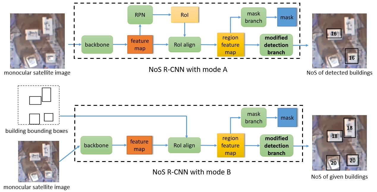
Mask R-CNN is a two-stage instance segmentation network proposed by Kaiming He in 2016. Without using any trick, Mask R-CNN achieved the best results in the 2016 Microsoft COCO object detection and instance segmentation competition. The core network architecture of Mask R-CNN is shown in Figure 1. The backbone network is responsible for generating a feature map based on the input image, and the region proposal network (RPN) generates category agnostic region of interest (RoI) based on the extracted feature map. RoI align extracts the features corresponding to RoI to get the regional feature map. These regional features will be sent to the detection branch for object classification and bounding box regression. Regional features based on the predicted region of detection branch will be sent to the mask branch for pixel level segmentation in the prediction stage.
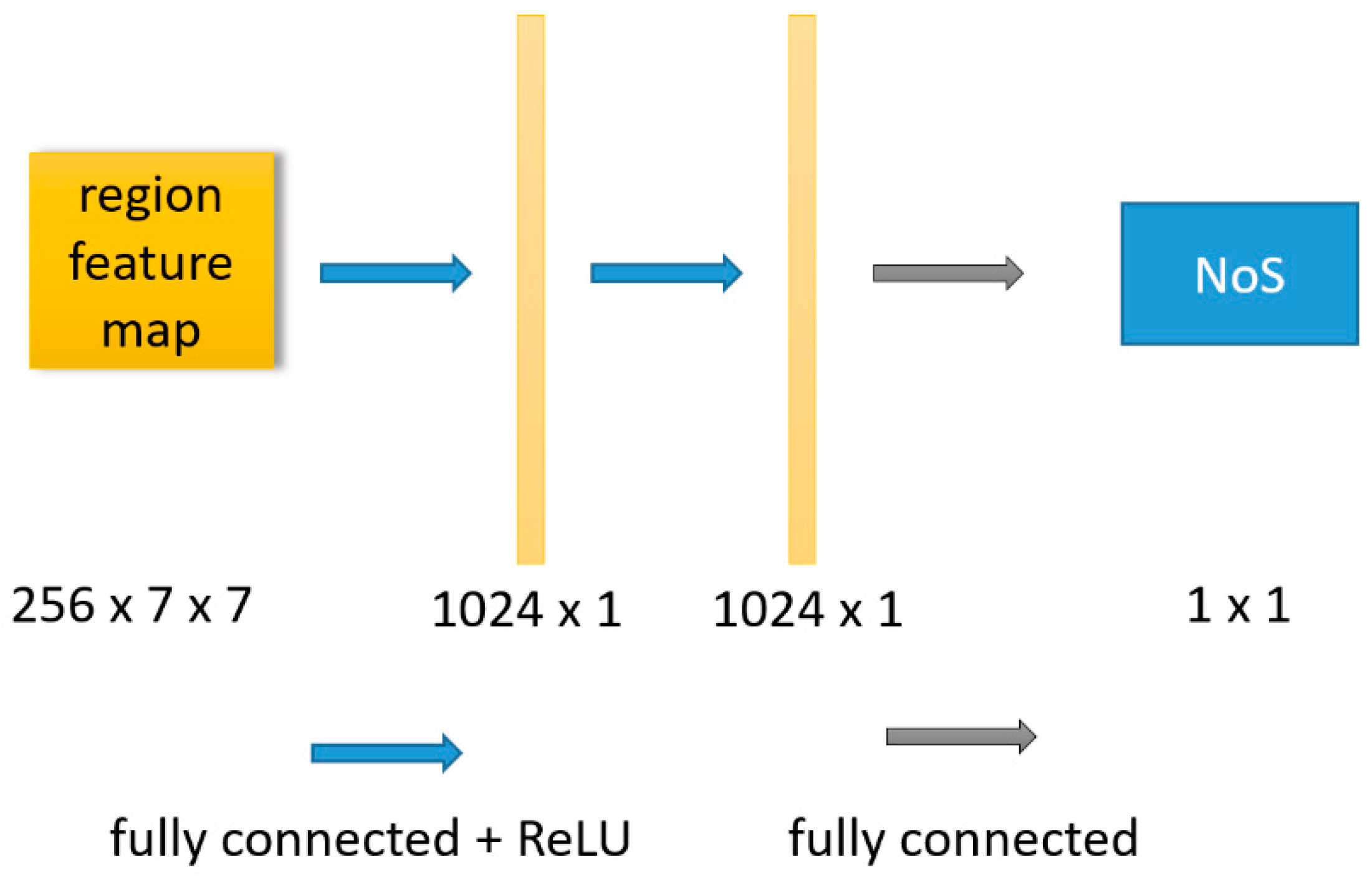
The network used in this paper is directly based on the resnet-50-fpn architecture described in [11]. Except for the modification of the detection branch (the red dotted line in the Figure 1), other structures are consistent with those in [11]. For the specific details of the base network, we recommend the reader to refer to [11]. In this section, we only describe the part of the base network that is modified. As shown in Figure 2, in detection branch, the regional features extracted by RoI align are represented as a feature vector with length of 1024 after passing through a two-layer fully connected network. The feature vector is shared by three tasks, i.e., object classification, bounding box regression, and NoS estimation. Finally, the shared feature vector obtains the respective output of three tasks through the full connected layer of three different tasks. The structure marked in the red box in the Figure 2 is the structure added in this paper, and the structure outside the red box is consistent with the detection branch of the original Mask R-CNN. In this paper, we call this method of integrating NoS estimation tasks by modifying detection branches as “detection branch integration”.
It should be pointed out that our model integrates the NoS estimation task, so compared with the input of original Mask R-CNN in training stage, our model needs the NoS ground truth of building objects as the supervision information. In addition, considering the scale of building object extraction, the goal of this paper is to extract the bounding box of building objects, so mask branch is not necessary in our network architecture. However, according to [11], to a certain extent, adding mask branch can improve the performance of the model in the object detection task, so we keep the mask branch, but do not consider the result of the mask branch in the model evaluation.
2.2. Two Kinds of Modes for Prediction
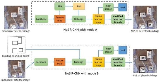
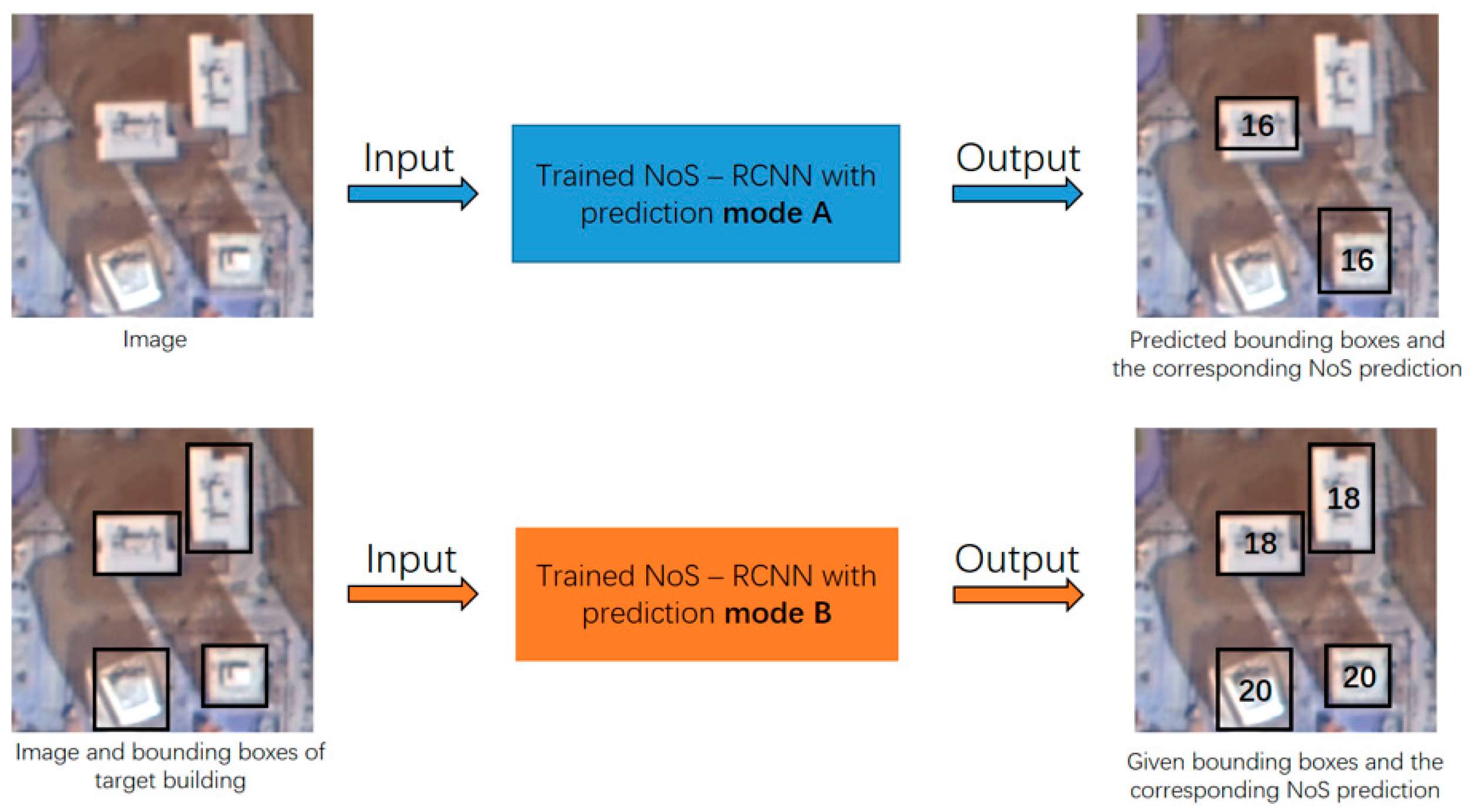
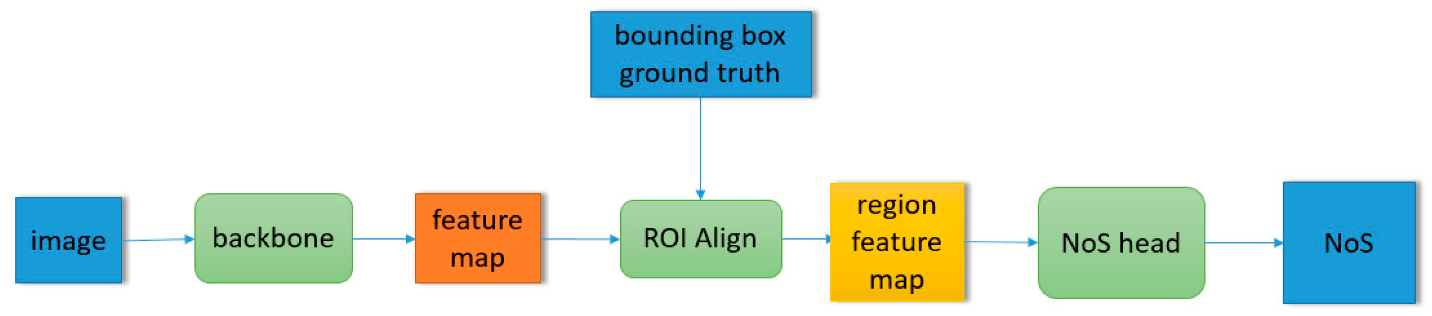
In the above network architecture, the set of building objects in the NoS estimation task is up to the result of building object detection task, which makes the application of the model have some limitations. For example, we cannot get the NoS estimation result of those objects that the model cannot detect. However, after a little modification of the above network architecture, the model can estimate NoS on the arbitrary given building object set, which makes the trained model have two prediction modes—mode A: in the prediction stage, the model inputs the monocular image, outputs the detection results of building objects and the corresponding NoS estimation results; mode B: in the prediction stage, the model inputs the monocular image and bounding box set of target buildings, outputs the given bounding boxes and the NoS estimation of the target buildings. The comparison of mode A and mode B is shown in Figure 3. Mode B expands the application scenarios of the model. The network architecture of mode B is shown in Figure 4. The input of RoI align is replaced the prediction of RPN with the given building bounding boxes. The “NoS head” shown in Figure 4 refers to the detection branch shown in Figure 2. In the detection branch, the prediction of the object detection task is replaced with the given building bounding boxes, and the corresponding NoS prediction is retained.
2.3. Loss Function
Our NoS estimation task is essentially a regression task, so we use the following loss function in the NoS estimation task:
where is the set of building objects whose true NoS information is known, and are the true value and predicted NoS of element i in , respectively. is the number of elements in . The function is consistent with the definition in [12]. The total loss of the network is defined as follows:
where is the total loss of the network, is the loss of original Mask R-CNN defined in [11], is the loss of NoS estimation task and is its weight.
3. Experiment
3.1. Dataset
Based on the aim of building detection and NoS estimation from monocular optical satellite image, we think that the detail information of building in low and medium resolution (i.e., 4 m or lower resolution) images is difficult to support the model to extract effective features for this task. Therefore, high resolution images should be used in the application of our methods. In this experiment, GF-2 multispectral data was used, the PanSharp algorithm [13] was used to fuse the multispectral data with panchromatic band, and its resolution was improved from 4 to 1 m. Three bands of red, green, and blue were used. We collected 9 GF-2 images covering nine large cities in China, such as Beijing, Guangzhou, and Xiamen, and their corresponding building contour vector data. Most of the building vector objects have NoS information. The building vector data was transformed into raster data of 1 m resolution as ground truth. Building bounding box ground truth was extracted from those raster ground truth. In order to facilitate the training, we divided all the images into patches with the size of 256 * 256 as experimental samples, and randomly divided the samples into training set and test set. Finally, 6202 training samples and 1551 test samples were obtained and there were 128,025 and 31,927 building objects with NoS information in the training set and test set, respectively. Figure 5a shows the geographical distribution of samples in the data set. Figure 5b shows a sample image in the data set and its corresponding ground truth, and Figure 5c shows the distribution of the number of buildings with different NoS on the training set and test set.
3.2. Implementation Details
In the experiment, the size of the batch is 16, SGD is used as the optimizer, learning rate is set to 0.001, and the λ in formula (2) is taken as 1. We integrate the NoS regression task on the Mask R-CNN model [14] which was pretrained on the COCO dataset, each subnetwork module was trained together during training stage. The threshold of nonmaximum suppression in the model is set to 0.3, and other parameters are consistent with those in [14]. As a small number of buildings in our dataset have no NoS information, this part of samples only participates in the loss calculation of object detection part in the training stage and model evaluation, but not in the loss calculation of the NoS prediction part.
3.3. Result
The experimental results should to be evaluated separately from both building detection task and NoS estimation task. However, in our method, we do not improve the original Mask R-CNN in the detection task. The building detection result is the carrier of the NoS estimation result, not the focus of this paper. Moreover, the problem of building detection using Mask R-CNN has been studied by many scholars [15,16,17,18,19]. Therefore, the performance of NoS estimation task will be taken as the center in the evaluation of experiments.
3.3.1. Building Detection Task
In the evaluation of the object detection task with only one target class, we assume that the predicted score of a predicted sample x is . To select a confidence threshold , predicted sample x is judged as a positive sample if is greater than , otherwise, a negative sample. For a positive sample and a ground truth sample , an IoU (Intersection over Union) threshold is selected, if the IoU of and is greater than the , then the pairing of and is successful and is called true positive (TP) sample. If fails to find the matching successful sample among all the ground truth samples, then is judged as the false positive (FP) sample. If fails to find the matching successful sample among all the predicted samples, will be judged as the false negative (FN) sample. We set that each predicted/ground truth sample can only match one ground truth/predicted sample successfully.
In the object detection competitions [20,21,22] such as COCO, the mean average precision (mAP) is often used as the evaluation metric, which can reflect the model’s average performance with multiple and . mAP is a fair evaluation metric which can fully measure the performance of the model in the competition. However, considering the research focus of this paper, for one thing, because building detection result is the carrier of the NoS estimation result and NoS estimation task can only be evaluated on TP samples, multiple and will make it difficult to evaluate the NoS estimation task. For another, in the actual application scenario of the model, we often choose to set the specific and for evaluation, not mutiple thresholds. Therefore, in this section, we set both and to 0.5 for the detection task and NoS estimation task.
We use precision, recall, and F1 score for building detection evaluation. The results are shown in Table 1.
3.3.2. NoS Estimation Task
In order to eliminate the influence of detection task performance and fully evaluate the real performance of the model in the NoS estimation task, we evaluate the results of the trained model in both A and B prediction modes. In the prediction results of mode A, only TP samples are evaluated. As described in Section 3.3.1, TP samples are determined with both and set to 0.5. In the prediction stage of prediction mode B, the images of test set and its corresponding bounding boxes ground truth are fed with the model, and all the building objects in the test set will be evaluated. Since mode B does not depend on the results of building object detection, the evaluation of prediction results in mode B can more accurately reflect the performance of the model in the NoS estimation task.
As mentioned above, the NoS estimation task is essentially a regression task, so we use the frequently used evaluation metrics. The mean absolute error (MAE) and mean relative error (nosIoU) on a set are as follows:
where is the predicted NoS of element which has the NoS ground truth in , is the NoS ground truth of . The function min (a, b) returns the minimum value of a and b, and represents the number of elements which have the NoS ground truth in . MAE measures the average value of the difference between the predicted value and the true value. As the dimension is maintained, this metric retains the physical meaning. The smaller the metric, the better the model performs. nosIoU uses the form of ratio and considers the relationship between the predicted value and the true value. Similar to the IoU in the two-dimensional image plane space used in detection task evaluation, nosIoU can be regarded as IoU in the one-dimensional space of NoS. The larger the metric, the better the performance of the model. According to the above formula, the metrics of the model on the test set are shown in Table 2, in which “@ TP” and “@ all” end with the evaluation of the prediction results of mode A and mode B, respectively. The row starting with “all” is the metrics on buildings which have NoS information. The rows starting with “low”, “middle”, and “high” are metrics on buildings whose number of stories is between 1–7, 8–20, and above 20. The values after “±” are the standard deviation. For example, the value of the first row and first column in the table is the MAE on true positive samples which have NoS information followed with the standard deviation of absolute error of those samples. The value of the second row and second column in the table is the MAE on all buildings in the test set whose NoS is between 1 and 7 followed with the standard deviation of absolute error of those samples.
In order to fully evaluate the prediction ability of the model on buildings with different NoS, we visualized the prediction results of the model on different NoS, as shown in Figure 6.
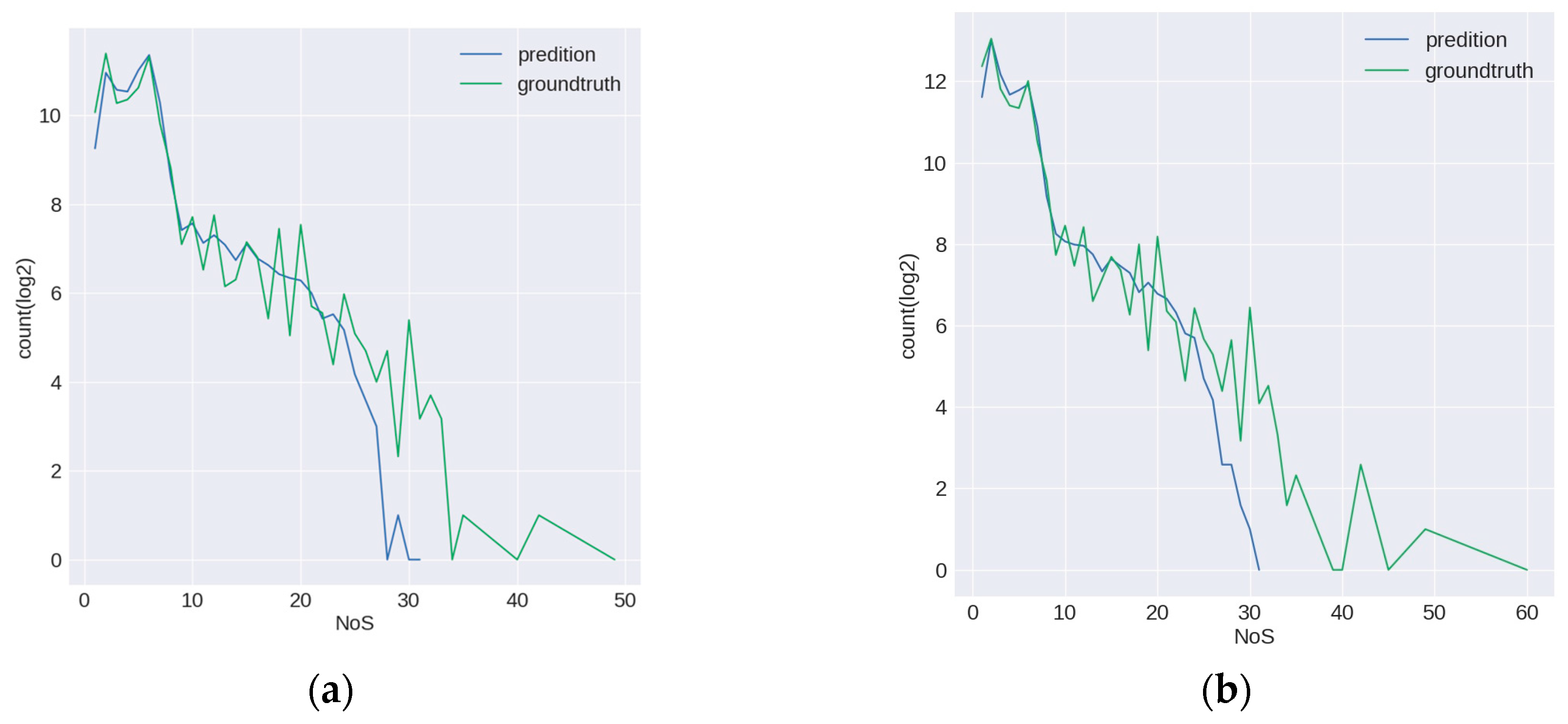
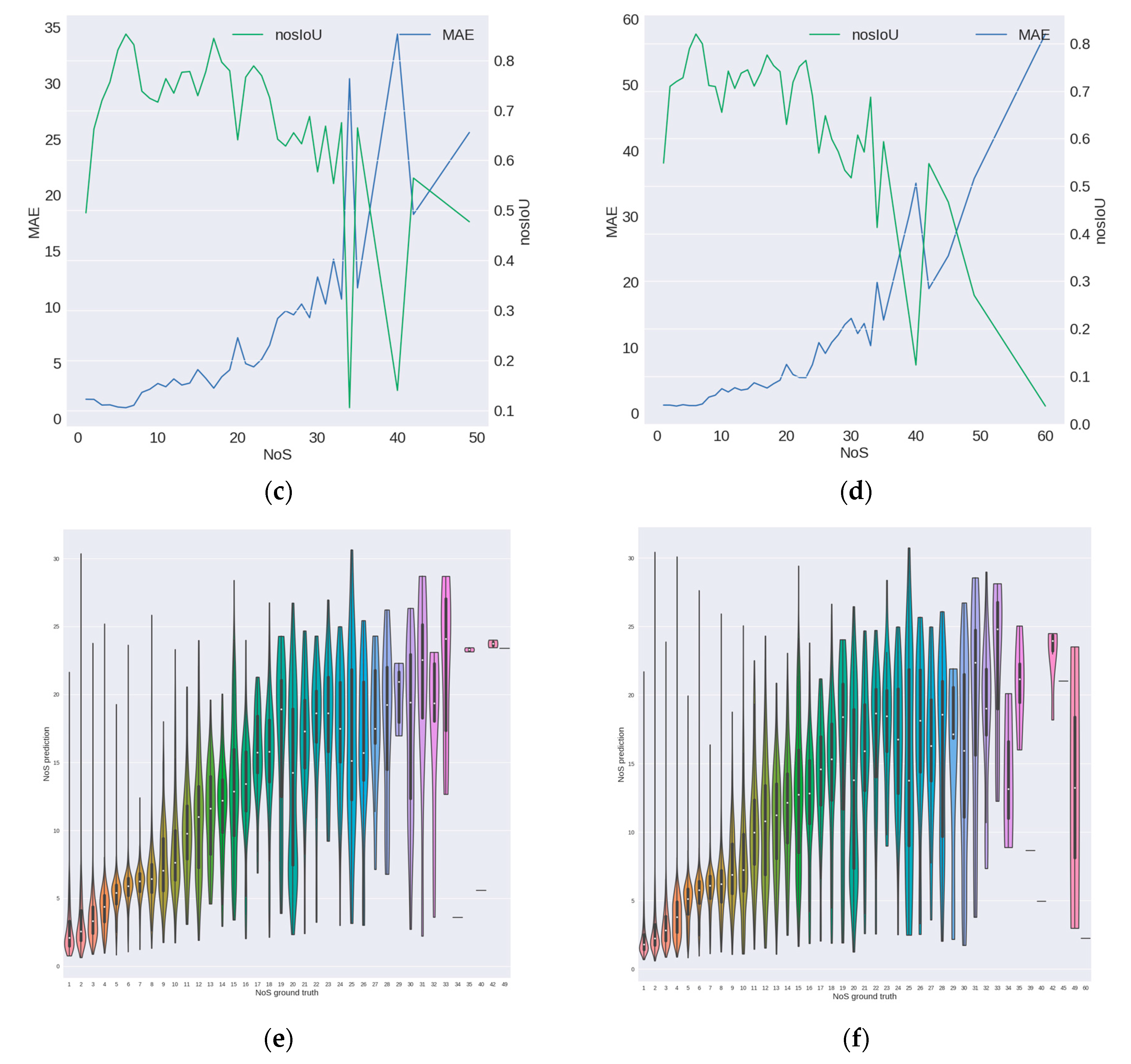
The results of the two prediction modes A and B are basically consistent in the overall trend of the three dimensions (i.e., the three rows in Figure 6). It can be seen from the first row of the figure that the distribution of prediction value below 10 stories is roughly consistent with the distribution of true value, but there is an increasing difference above 10 stories. Although there are some samples with more than 30 stories in the test samples, the prediction of the model hardly contains the prediction value of more than 30 stories. At the same time, it should be noted that the number of samples above 30 stories is small in both model A and model B, so the metrics on this part of samples are almost not statistically significant. From the second row, we can see that the for low-rise samples, MAE is relatively small, and MAE of mode A is a little bigger than that of mode B. The nosIoU on low-rise samples is relatively low because this metric considers the values of error and NoS simultaneously. The two metrics on middle-rise samples are relatively stable, but the error on those is bigger. For high-rise buildings, the two metrics are unstable and the error on those is much bigger. From the overall trend, it can be seen that with the increase of the number of stories, the performance of the model on both metrics is getting worse and worse. The similar trends can be found in Table 2. From the third row, it can be seen that the distribution of the predicted values in the low-rise buildings are relatively concentrated, which indicate that the performance of the model on low-rise buildings is stable, while the predicted values on the high-rise buildings are relatively scattered, and the median of the predicted value is often lower than the corresponding true value. Combined with Figure 5c, we can see that in the training set, the number of building samples decreases as the NoS increases, and the number of high-rise samples is much lower than that of the low-rise samples. Besides the difficulty of the task itself (i.e., lack of the obvious features on the image for NoS estimation task), lack of sufficient samples may be one of the reasons leading to the larger prediction error of the model on high-rise samples. Figure 7 shows some prediction results of the model on the test samples. It can be seen that the results on the low-rise buildings are surprisingly good considering that it is extremely difficult for ordinary people, but the results on high-rise buildings are unsatisfactory.
4. Discussion
Under the technical aspect of this paper regarding modifying an object detection network to integrate the building detection task and the NoS estimation task at the same time, the choice of the integration method and the interaction between building detection task and NoS estimation task are worth discussing. In Section 4.1 and Section 4.2, we will discuss the above problems through experiments. In Section 4.3, we will discuss the decision basis of the model, which is maybe the most controversial part of the study.
4.1. Choice of Integration Mode
In order to achieve the objectives of this study, in addition to the integration mode described in Section 2 (i.e., “detection branch integration”), another natural and direct mode of integration is to add a separate branch for the NoS estimation task, as shown in the red dashed-line frame part in Figure 8, which is parallel to the detection branch and called “NoS branch”. NoS branch is trained and inferred in a manner consistent with the mask branch [11]. In this article, we call this method of integrating NoS estimation tasks by adding new branches paralleled to detection branches as “NoS branch integration”. To compare the performance differences between different integration modes and to explore the interaction between detection tasks and NoS estimation tasks in this multitask learning architecture, we conducted three supplementary experiments to compare the results from the “detection branch integration” experiment in Section 3, which was set up as follows:
- Detection benchmark. Using the same network architecture as “detection branch integration”, λ in formula (2) was set to 0 in training stage. In this setting, the total loss of the network only includes the loss defined in the original Mask R-CNN and does not include the loss of NoS estimation task.
- GT proposal benchmark. Using the same network architecture as “detection branch integration”. In training stage, the input of RoI align is replaced by the predicted value of RPN with the building bounding box ground truth. The “NoS head” shown in Figure 4 is the detection branch. The total loss of the network only retains the loss of NoS estimation task.
- NoS branch. Using the architecture shown in Figure 8 and Figure 9. In order to maintain the comparability between experiments, the specific network architecture of NoS branch which is shown in Figure 9 remains similar to detection branch which is shown in Figure 2 in “detection branch integration”. In prediction stage with mode B, “NoS head” in Figure 4 is NoS branch. The loss function of the network is consistent with that in “detection branch integration”.
The above three groups of experiments use the same training conditions (e.g., training set, hyper parameters) as the experiment in Section 3, and evaluate them on the same test set. The results can be seen in Table 3:
- The performance of “detection branch integration” and “NoS branch integration” is similar in both detection task and NoS estimation task, “NoS branch integration” performs slightly better in the detection task, while “detection branch integration” performs slightly better in the NoS estimation task.
- Compared with the “detection benchmark” which only retains the detection task, the performance in the detection task of the two networks integrated with NoS estimation task is slightly lower than the former, but there is no obvious degradation.
- By comparing the performance of the two integration methods and the “GT proposal benchmark”, which only retains the NoS estimation task and fed with the accurate bounding box for RoI align in training stage, we can see that the former is better than the latter, which indicates that the end-to-end training of NoS estimation task with the detection task in the training stage can help the model obtain better performance in the NoS estimation task. It should be pointed out that because the “GT proposal benchmark” does not learn for the detection task in the training stage, only “MAE@all” and “nosIoU@all” have reference significance.
4.2. The Impact of Detection Task on NoS Estimation Task
For one thing, in the prediction mode A, building detection result is the carrier of the NoS estimation result. For another, from the perspective of network architecture, two tasks share most of the parameters of network and regional features, so it is of great significant to further explore the impact of detection tasks on NoS estimation tasks.
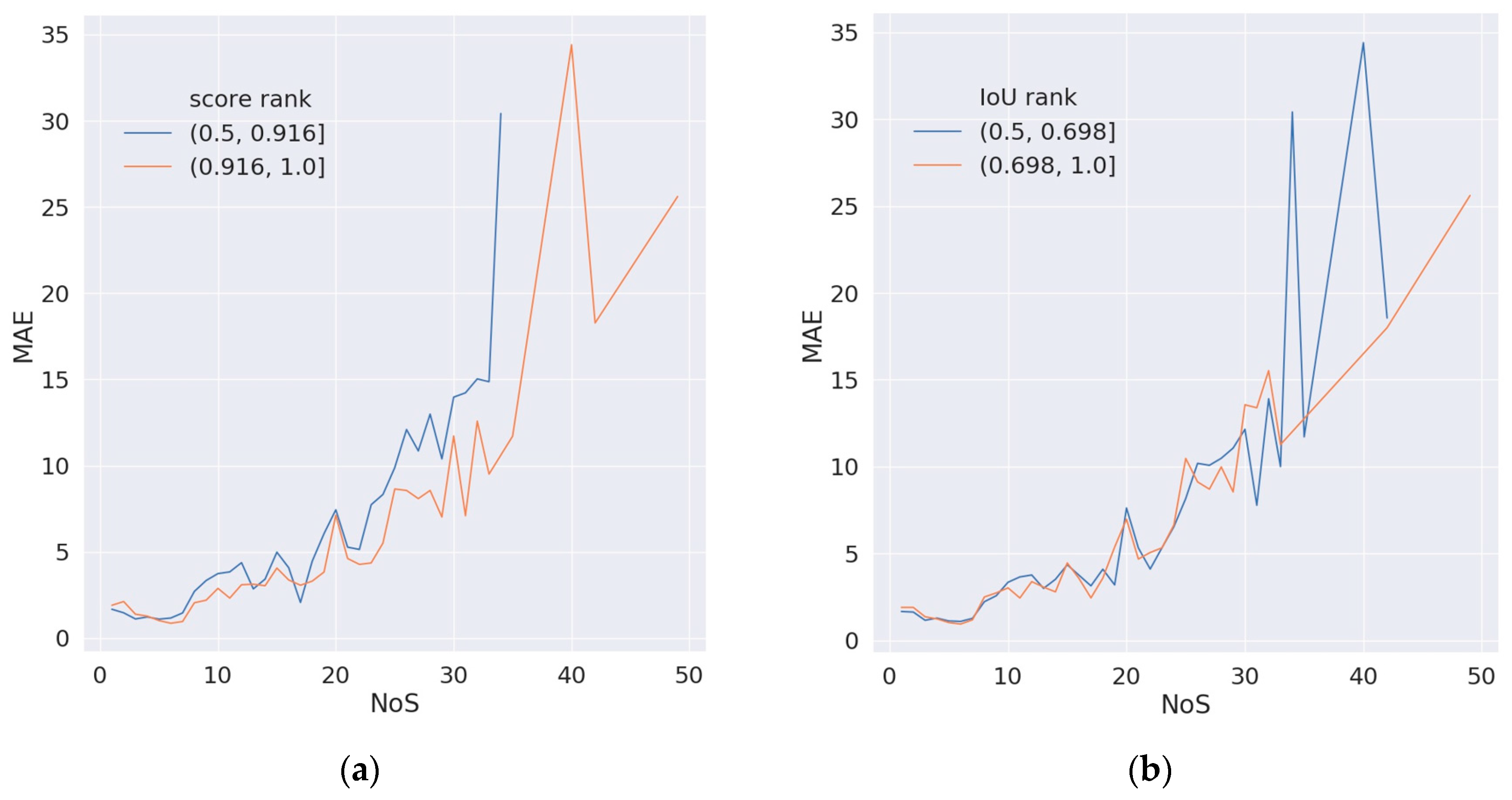
In the detection task, the model will give a score on each predicted object to represent the confidence degree that the predicted object belongs to the target class. The IoU of the predicted bounding box and the ground truth is calculated to represent the location accuracy on the predicted value. In order to explore the relationship between the score/IoU of the detection task and the accuracy of the NoS estimation task, we analyzed the TP samples predicted by the trained detection branch integration model in prediction mode A, in which the task accuracy of the NoS estimation was represented by MAE metric. Take the relationship between score and MAE as an example: taking the median of predicted score 0.916 on all TP samples as the threshold value, the TP samples are divided into two subsets (0.5, 0.916) and (0.916, 1.0) with almost equal number of samples, and draw the distribution of NoS and MAE on the two subsets. The relationship between IoU and MAE is analyzed in the same way, and the results are shown in Figure 10.
It can be seen that for score, the MAE distribution curve of the subset with high score is under the subset with low score in most of the horizontal axis, which indicates that the prediction result of high score on the TP sample is often relatively low, that is, it has higher accuracy in the NoS estimation task. For IoU, the curves of the two subsets are intertwined in most of the horizontal axis, and there is no obvious advantage of a subset. Therefore, there is no clear relationship between the location accuracy of detection task and the accuracy of NoS estimation on TP samples.
4.3. The Decision Basis of the Model
Like the task of depth estimation from monocular images in the field of computer vision, the physical mechanism of our method is still unclear. Therefore, we call the predicted result of our model as a kind of estimation rather than the accurate measurement. It is generally believed that deep convolution neural network (DCNN) can end-to-end mine features supporting the target tasks and learn corresponding knowledge and rules by learning from a large number of samples. Therefore, although ordinary people cannot summarize the definite knowledge or rules from the image for NoS estimation, but from our experiment results, the model shows the learning ability and generalization ability to some extent, so we think that there should be some meaningful features in the image to support the model to make decision. In this section, we try to analyze the features that are meaningful to the task of NoS estimation:
- The feature of building itself, including the shape, size, color, and texture of the roof of building reflected in the image. Although these features may not determine the NoS from the physical side, they may have some statistical significance. For example: buildings with very large or small roof areas are often not high-rise buildings. It should be pointed out that the image used in our experiment is 1 m resolution ortho-rectifying satellite image. We cannot see any side information of buildings even for the high-rise building from our image, such as windows or balconies of buildings (as can be seen in Figure 7). Therefore, our model does not use the side information of buildings. However, we believe that the side information of buildings in the appropriate image should play a more important role in the task of NoS estimation, but this point might need to be furthermore tested in the future related research.
- Context features around the building. Although the bounding box of the building itself for RoI align is utilized to extract the region feature of building in our method, the region feature of building was cropped by RoI align from the feature map which is convoluted by many layers of backbone. Every pixel in feature maps has a larger and larger receptive field in the process of forward computation. Therefore, the receptive field of region features extracted by RoI align is much larger than the corresponding bounding box and the region feature can contain the information outside the bounding box. This is different from the methods of cropping the local image based on bounding box first and then extracting its features, of which the receptive field cannot outside the bounding box. We call the information outside the bounding box as the context information, and we think that there are two kinds of context information that are meaningful for NoS estimation:
- (a)
- The shadow of buildings. The length of building shadow reflects the height of the building to a certain extent, and the height of the building has a high correlation with NoS. In a certain scene, the NoS of buildings with relatively long shadows are often bigger than that of buildings with relatively short shadows.
- (b)
- The relationship between adjacent building objects and the environment of buildings. For example: buildings with adjacent locations and similar roof features often belong to the same community, and they often have the same NoS. The possibility that high-rise buildings appear in suburbs or farmland is very low.
The above analysis is only some conjectures about the possible internal mechanism of this method, and most of them are only of statistical significance. A clear understanding of the meaningful features extracted by the model and the learned decision rules depends on people’s fundamental understanding of the working mechanism of DCNN.
5. Conclusions
In this paper, we proposed a multitask integration approach which detects building objects and estimates NoS simultaneously from monocular optical satellite images based on Mask R-CNN. Through the verification on the images of nine large cities in China, it was shown that MAE and nosIoU of test set was 1.83 and 0.74, respectively. The mean absolute error of prediction on buildings whose number of stories is between 1–7, 8–20, and above 20 are 1.329, 3.546, and 8.317 respectively, which indicates that the prediction error of this method is relatively small on low-rise buildings, but it is large on medium-rise and high-rise buildings, which needs further improvement However, considering that the task is still very difficult even if the task is handed over to human beings, and the related research of building NoS estimation based on deep learning methods from monocular optical satellite images is still in the beginning stage, so this study has great development potential and promotion space. In addition to the feature of the building itself, the shadow of the building in the image is also closely related to the height and NoS of buildings, but the relevant information is not explicitly used in this method. How to effectively use the shadow feature of buildings to improve the accuracy of the NoS estimation method in this paper (especially in high-rise buildings) will be an important direction of further research in this paper.
Author Contributions
Conceptualization, H.T.; Funding acquisition, H.T.; Investigation, H.T. and C.J.; Methodology, C.J.; Software, C.J.; and Supervision, H.T. All authors have read and agreed to the published version of the manuscript.
Funding
This work was supported by the National Natural Science Foundation of China (No. 41971280) and the National Key R&D Program of China (No. 2017YFB0504104).
Acknowledgments
We would like to thank the high-performance computing support from the Center for Geodata and Analysis, Faculty of Geographical Science, Beijing Normal University (https://gda.bnu.edu.cn/).
Conflicts of Interest
The authors declare no conflict of interest.
References
- Ning, W. Study on 3D Reconstruction for City Buildings Based on Target Recognition and Parameterization Technology; Zhejiang University: Hangzhou, China, 2013. [Google Scholar]
- Mou, L.; Zhu, X.X. IM2HEIGHT: Height estimation from single monocular imagery via fully residual convolutional-deconvolutional network. arXiv 2018, arXiv:1802.10249. [Google Scholar]
- Paoletti, M.E.; Haut, J.M.; Ghamisi, P.; Yokoya, N.; Plaza, J.; Plaza, A. U-IMG2DSM: Unpaired Simulation of Digital Surface Models with Generative Adversarial Networks. IEEE Geosci. Remote Sens. Lett. 2020. [Google Scholar] [CrossRef]
- Shao, Y.; Taff, G.N.; Walsh, S.J. Shadow detection and building-height estimation using IKONOS data. Int. J. Remote Sens. 2011, 32, 6929–6944. [Google Scholar] [CrossRef]
- Liasis, G.; Stavrou, S. Satellite images analysis for shadow detection and building height estimation. ISPRS J. Photogramm. Remote Sens. 2016, 119, 437–450. [Google Scholar] [CrossRef]
- Raju PL, N.; Chaudhary, H.; Jha, A.K. Shadow analysis technique for extraction of building height using high resolution satellite single image and accuracy assessment. In Proceedings of the International Archives of the Photogrammetry, Remote Sensing & Spatial Information Sciences, Hyderabad, India, 9–12 December 2014. [Google Scholar]
- Srivastava, S.; Volpi, M.; Tuia, D. Joint height estimation and semantic labeling of monocular aerial images with CNNs. In Proceedings of the 2017 IEEE International Geoscience and Remote Sensing Symposium (IGARSS), Fort Worth, TX, USA, 23–28 July 2017; IEEE: Piscataway, NJ, USA, 2017; pp. 5173–5176. [Google Scholar]
- Ghamisi, P.; Yokoya, N. Img2dsm: Height simulation from single imagery using conditional generative adversarial net. IEEE Geosci. Remote Sens. Lett. 2018, 15, 794–798. [Google Scholar] [CrossRef]
- Amirkolaee, H.A.; Arefi, H. Height estimation from single aerial images using a deep convolutional encoder-decoder network. ISPRS J. Photogramm. Remote Sens. 2019, 149, 50–66. [Google Scholar] [CrossRef]
- Amirkolaee, H.A.; Arefi, H. Convolutional neural network architecture for digital surface model estimation from single remote sensing image. J. Appl. Remote Sens. 2019, 13, 016522. [Google Scholar] [CrossRef]
- He, K.; Gkioxari, G.; Dollar, P.; Girshick, R. Mask r-cnn. In Proceedings of the IEEE International Conference on Computer Vision, Venice, Italy, 22–29 October 2017; pp. 2961–2969. [Google Scholar]
- Girshick, R. Fast r-cnn. In Proceedings of the IEEE International Conference on Computer Vision, Araucano Park, Las Condes, Chile, 11–18 December 2015; pp. 1440–1448. [Google Scholar]
- Zhang, Y.; Mishra, R.K. From UNB PanSharp to Fuze Go–the success behind the pan-sharpening algorithm. Int. J. Image Data Fusion 2014, 5, 39–53. [Google Scholar] [CrossRef]
- Marcel, S.; Rodriguez, Y. Torchvision the machine-vision package of torch. In Proceedings of the 18th ACM International Conference on Multimedia, Firenze, Italy, 25–29 October 2010; pp. 1485–1488. [Google Scholar]
- Zhao, K.; Kang, J.; Jung, J.; Sohn, G. Building Extraction from Satellite Images Using Mask R-CNN With Building Boundary Regularization. In Proceedings of the CVPR Workshops, Salt Lake City, UT, USA, 18–22 June 2018; pp. 247–251. [Google Scholar]
- Zhang, L.; Wu, J.; Fan, Y.; Gao, H.; Shao, Y. An Efficient Building Extraction Method from High Spatial Resolution Remote Sensing Images Based on Improved Mask R-CNN. Sensors 2020, 20, 1465. [Google Scholar] [CrossRef] [Green Version]
- Zhou, K.; Chen, Y.; Smal, I.; Lindenbergh1et, R. Building segmentation from airborne vhr images using mask R-cnn. In Proceedings of the International Archives of the Photogrammetry, Remote Sensing & Spatial Information Sciences, Enschede, The Netherlands, 10–14 June 2019. [Google Scholar]
- Stiller, D.; Stark, T.; Wurm, M.; Dech, S.; Taubenböck, H. Large-scale building extraction in very high-resolution aerial imagery using Mask R-CNN. In Proceedings of the 2019 Joint Urban Remote Sensing Event (JURSE), Vannes, France, 22–24 May 2019; IEEE: Piscataway, NJ, USA, 2019; pp. 1–4. [Google Scholar]
- Hu, Y.; Guo, F. Building Extraction Using Mask Scoring R-CNN Network. In Proceedings of the 3rd International Conference on Computer Science and Application Engineering, Sanya, China, 22–24 October 2019; pp. 1–5. [Google Scholar]
- Lin, T.Y.; Maire, M.; Belongie, S.; Hays, J.; Perona, P.; Ramanan, D.; Dollár, P.; Zitnick, C.L. Microsoft coco: Common objects in context. In Proceedings of the European Conference on Computer Vision, Zurich, Switzerland, 6–12 September 2014; Springer: Cham, Switzerland, 2014; pp. 740–755. [Google Scholar]
- Everingham, M.; Van Gool, L.; Williams, C.K.; Winn, J.; Zisserman, A. The pascal visual object classes (voc) challenge. Int. J. Comput. Vis. 2010, 88, 303–338. [Google Scholar] [CrossRef] [Green Version]
- Shao, S.; Li, Z.; Zhang, T.; Peng, C.; Yu, G.; Zhang, X.; Li, J.; Sun, J. Objects365: A large-scale, high-quality dataset for object detection. In Proceedings of the IEEE International Conference on Computer Vision, Seoul, Korea, 27 October–2 November 2019; pp. 8430–8439. [Google Scholar]
Figure 1.
Schematic diagram of Mask R-CNN core network architecture.

Figure 2.
Schematic diagram of integration of NoS estimation task in detection branch.

Figure 3.
Schematic diagram of mode A and mode B.

Figure 4.
Schematic diagram of perdition stage of mode B.

Figure 5.
Data set. (a) The geographical distribution of samples in the data set. (b) The sample image and ground truth. The green labels in (b) are the building mask ground truth used in mask branch training, the bounding boxes are the bounding box ground truth, and the number on bounding boxes are NoS ground truth. (c) The distribution of the number of buildings with different NoS, whose vertical axis carried out logarithm transformation based on 2.

Figure 6.
Distribution of evaluation metrics on different NoS. The left and right columns are the results of mode A and mode B, respectively. The first row, i.e., subfigures (a,b), reflects the quantitative distribution of predicted value and true value on different NoS, and on its vertical axis logarithm transformation was carried out based on 2; the second row, i.e., subfigures (c,d), reflects the distribution of MAE and nosIoU on different NoS; the third row, i.e., subfigures (e,f), is the violin diagram of predicted value of NoS, reflecting the distribution of predicted values on different NoS.


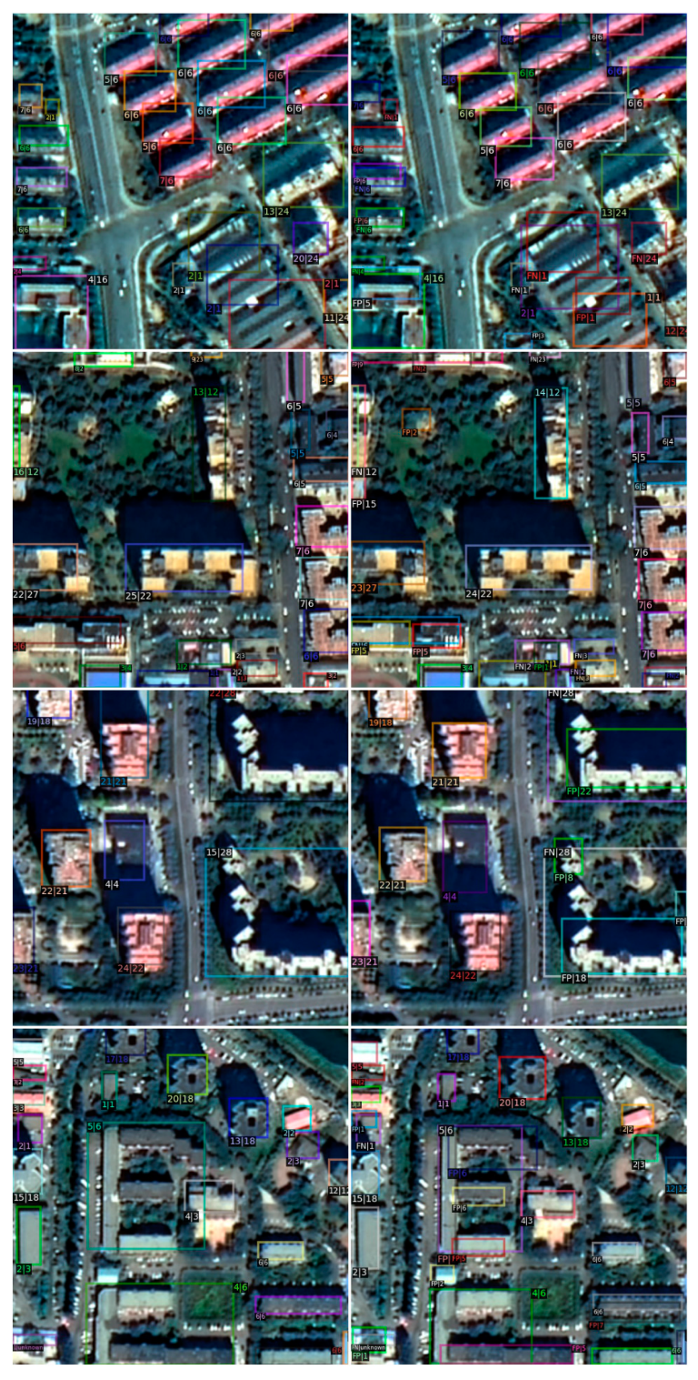
Figure 7.
Prediction results of the model on the test set. The four rows show the results on different regions. The left column shows the prediction of mode B, and the right column shows the “TP”, “FP”, and “FN” prediction of mode A. The color of the bounding boxes has no specific meaning, just in order to distinguish different objects. Most bounding boxes have a pair of numbers separated by “|”. The first number is the NoS prediction of the model and the second is the NoS ground truth. The boxes with pairs start with “FP”/ “FN” are “FP”/”FN” objects and the numbers of those are predicted/true NoS. All predicted values shown in the figure have been rounded up or rounded down to the nearest decimal. For example, a bounding box with the label “4|6” indicates that the bounding box is the prediction of a “true positive” sample whose NoS prediction and ground truth is 4 and 6, respectively. A bounding box with the label “FP|3” indicates that the bounding box is the prediction of a “false positive” sample whose NoS prediction is 3. A bounding box with the label “FN|1” indicates that the bounding box is the ground truth of a “false negative” sample whose NoS ground truth is 1.

Figure 8.
Diagram of network architecture of “NoS branch integration”.

Figure 9.
Diagram of network architecture of the NoS branch.

Figure 10.
Distribution of MAE on different NoS. (a) shows the distribution of subsets of predictions with low score and high score. (b) shows the distribution of subsets of predictions with low IoU and high IoU.
Figure 10.
Distribution of MAE on different NoS. (a) shows the distribution of subsets of predictions with low score and high score. (b) shows the distribution of subsets of predictions with low IoU and high IoU.


Table 1.
Building detection evaluation metrics.
| F1 | Precision | Recall |
|---|---|---|
| 0.449 | 0.482 | 0.421 |
Table 2.
NoS estimation evaluation metrics.
| MAE@TP | MAE@all | nosIoU@TP | nosIoU@all | |
|---|---|---|---|---|
| All | 1.833 ± 2.67 | 1.673 ± 2.58 | 0.740 ± 0.21 | 0.709 ± 0.21 |
| Low | 1.329 ± 1.85 | 1.257 ± 1.73 | 0.742 ± 0.21 | 0.711 ± 0.21 |
| Middle | 3.546 ± 3.27 | 3.886 ± 3.42 | 0.739 ± 0.20 | 0.708 ± 0.22 |
| High | 8.317 ± 6.18 | 9.926 ± 7.32 | 0.687 ± 0.21 | 0.635 ± 0.24 |
Table 3.
Experiments evaluation metrics.
| F1 | Precision | Recall | MAE@TP | MAE@all | nosIoU@TP | nosIoU@all | |
|---|---|---|---|---|---|---|---|
| Detection Benchmark | 0.458 | 0.482 | 0.437 | 5.90 | 4.656 | 0.026 | 0.030 |
| GT proposal benchmark | 0.033 | 0.020 | 0.090 | 1.642 | 1.739 | 0.675 | 0.698 |
| Detection branch integration | 0.449 | 0.483 | 0.420 | 1.833 | 1.673 | 0.740 | 0.709 |
| NoS branch | 0.451 | 0.480 | 0.426 | 1.827 | 1.676 | 0.739 | 0.707 |
Publisher’s Note: MDPI stays neutral with regard to jurisdictional claims in published maps and institutional affiliations. |
© 2020 by the authors. Licensee MDPI, Basel, Switzerland. This article is an open access article distributed under the terms and conditions of the Creative Commons Attribution (CC BY) license (http://creativecommons.org/licenses/by/4.0/).
Share and Cite
MDPI and ACS Style
Ji, C.; Tang, H. Number of Building Stories Estimation from Monocular Satellite Image Using a Modified Mask R-CNN. Remote Sens. 2020, 12, 3833. https://0-doi-org.brum.beds.ac.uk/10.3390/rs12223833
AMA Style
Ji C, Tang H. Number of Building Stories Estimation from Monocular Satellite Image Using a Modified Mask R-CNN. Remote Sensing. 2020; 12(22):3833. https://0-doi-org.brum.beds.ac.uk/10.3390/rs12223833
Chicago/Turabian StyleJi, Chao, and Hong Tang. 2020. "Number of Building Stories Estimation from Monocular Satellite Image Using a Modified Mask R-CNN" Remote Sensing 12, no. 22: 3833. https://0-doi-org.brum.beds.ac.uk/10.3390/rs12223833
Note that from the first issue of 2016, this journal uses article numbers instead of page numbers. See further details here.