Article

Using GIS and Machine Learning to Classify Residential Status of Urban Buildings in Low and Middle Income Settings

by
Christopher T. Lloyd
1,*,
Hugh J. W. Sturrock
2,
Douglas R. Leasure
1,
Warren C. Jochem
1,
Attila N. Lázár
1 and
Andrew J. Tatem
1
1
WorldPop Programme, Department of Geography and Environmental Science, University of Southampton, Southampton SO17 1BJ, UK
2
Locational, Lytchett House, 13 Freeland Park, Wareham Road, Poole BH16 6FA, UK
*
Author to whom correspondence should be addressed.
Remote Sens. 2020, 12(23), 3847; https://0-doi-org.brum.beds.ac.uk/10.3390/rs12233847
Submission received: 28 August 2020 / Revised: 13 November 2020 / Accepted: 19 November 2020 / Published: 24 November 2020
(This article belongs to the Special Issue Remote Sensing Application to Population Mapping)

Abstract

:
Utilising satellite images for planning and development is becoming a common practice as computational power and machine learning capabilities expand. In this paper, we explore the use of satellite image derived building footprint data to classify the residential status of urban buildings in low and middle income countries. A recently developed ensemble machine learning building classification model is applied for the first time to the Democratic Republic of the Congo, and to Nigeria. The model is informed by building footprint and label data of greater completeness and attribute consistency than have previously been available for these countries. A GIS workflow is described that semiautomates the preparation of data for input to the model. The workflow is designed to be particularly useful to those who apply the model to additional countries and use input data from diverse sources. Results show that the ensemble model correctly classifies between 85% and 93% of structures as residential and nonresidential across both countries. The classification outputs are likely to be valuable in the modelling of human population distributions, as well as in a range of related applications such as urban planning, resource allocation, and service delivery.

Graphical Abstract

1. Introduction

The UN Sustainable Development Goals (SDGs) highlight that urban areas in lower income settings each have unique development needs associated with human health, livelihoods, changes in family patterns, and the local environment [1,2]. Consequently, urban areas require more detailed, disaggregated population data in local contexts in order to monitor and tackle such issues [3]. In low and middle income countries, however, vital registration is nonexistent, and population and housing censuses often have less than decadal frequencies. Where there is an absence of recent population and housing census data, population models can provide high resolution and reliable estimates of population distribution [4]. It has been demonstrated that covariates which express settlement characteristics (or proxies for these, e.g., night time light brightness, impervious surface mapping) are able to inform population models most effectively [5,6,7]. However, there is a need for greater recognition of the whereabouts of residential and nonresidential building types, particularly in urban areas which have varying residential and socioeconomic characteristics. When population models are better informed by such data, it is possible to equip national, regional, and local levels of government (or nongovernmental organisations or private subcontractors) with more accurate datasets of population distribution. These are essential in order to ensure successful management of urban areas, resource allocation, and service delivery. Further, to obtain modelled predictions of building type is preferable to time consuming and labour intensive manual delineation of such settlement characteristics from imagery using human operators. Modelling is also necessary because building footprint data (i.e., an assemblage of building outlines) rarely provide details pertaining to building type unless linked to property or personal attribute data. An exception to this is if the source settlement dataset is volunteered geographic information (VGI), such as open source OpenStreetMap (OSM), where incomplete and inconsistent labelling may be present.
As discussed by Jochem et al. [8], settlement models using geospatial vector data (points, lines, polygons) have shown the potential to identify building type or urban land uses [9,10]. Such data are routinely assembled by commercial cartographic organisations, by volunteers (i.e., VGI), and increasingly by the ‘Big Tech’ companies, with vector polygons most used to delineate the geometry of buildings (i.e., building footprints). However, in some datasets each individual building is represented only by a single point, often with significant error margins on building location. Barr et al. [10] distinguish between morphological properties (e.g., area, orientation, or compactness) and spatial relations (e.g., proximity or connectivity between polygons) to organise shape measurements. At a localised scale, the geospatial characteristics of many polygon geometries together (and, to a much more limited extent, point geometries) are useful in forming a pattern that can be harnessed by machine learning algorithms in decision making. Such patterns allow the algorithm to identify broad features within the built landscape and so allow determination of probable land use.
Quantifiable patterns provide a route to improve automated land use classifications [11]. Several previous studies aimed to identify building use and to automate map generalisation [8,9,12,13,14,15,16,17]. Sturrock et al. [18] focus on the binary classification of building footprint data into residential and nonresidential building types, in data poor urban areas across each of two low/middle income countries. Their study applies the principles of stacked generalisation, as established by Wolpert [19], in an ensemble machine learning approach in order to classify building function within urban areas. The work broadly builds upon that of Lu et al. [20] and Xie and Zhou [21]. Data inputs are OSM building footprint and highway (© 2017 OpenStreetMap contributors; geofabrik.de) datasets, and an impervious surface dataset for Africa [22]. OSM highway input includes all roads available within the dataset per country. Training and testing of the model employs building structure attribute labels contained in the building footprints. A variety of commonplace building or urban morphological properties and spatial relations are calculated by the model as predictor variables in order to inform predictions.
This paper describes a newly developed GIS workflow that performs the extensive processing necessary to input new building footprint and label data to the recently developed building classification model of Sturrock et al. [18]. The model is applied to urban areas in two new case study countries—the Democratic Republic of the Congo (COD), and Nigeria (NGA). The workflow is designed to be particularly useful to those who apply the model to additional countries and use input data from diverse sources, especially as separate footprint and label data become more widely available in the future. We elucidate and discuss the statistical and visualised, real world (i.e., human operator checked) performance of the model for each country, illustrated by use of selected classified building footprint outputs. We compare the statistical outputs to those of Sturrock et al. [18].

2. Materials and Methods

2.1. Source Datasets

Although building footprints are becoming more commonly available for low and middle income countries, coverage can be patchy and completeness within areas of coverage can be poor—particularly in open source data (such as OSM). Further, the lack of label data is currently often a barrier to satisfactory building classification modelling performance. The case study countries (COD and NGA) were selected based on availability of additional, new (licensed and open), building footprint and label data of improved coverage, completeness, and attribute consistency. Further, the case studies were selected for being similar and proximal low and middle income settings to those explored by Sturrock et al. [18], with similar spatial distribution of urban centres. This allows useful comparisons to be drawn between the two studies, of the statistical outputs of the building classification model.
Data inputs to the GIS workflow, for eventual ingestion to the model, are Maxar Technologies (DigitizeAfrica data © 2020 Maxar Technologies, Ecopia.AI) building footprint (vector polygon) data, and OSM building footprints (vector polygon) and building attribute labels (© 2020 OpenStreetMap contributors; geofabrik.de). Further inputs are the World Bank [23], Oak Ridge National Laboratory (ORNL) [24], eHealth Africa and WorldPop (University of Southampton) [25], and University of California–Los Angeles and Kinshasa School of Public Health (UCLA and KSPH) [26] manually field mapped building attribute (vector point) labels. OSM highway (vector line) data (acquired in January 2020) were input directly into the model without the need for processing by GIS workflow. Values were extracted (at individual building footprint locations) from raster US NASA (SEDAC) Global Man-made Impervious Surface (GMIS) Landsat data [27] and converted into tabular data by the GIS workflow for input to the model. Input highway and impervious data allow the calculation of some advanced predictor variables for use in the model, such as distance of structure to nearest road, and urbanicity, discussed in Section 2.2. Source datasets used as input to the building classification model, either via the GIS workflow or directly, are summarized in Table 1.
The label datasets map building use (usually simply denoted as residential or nonresidential). The World Bank dataset originates from a regional electrification survey and has coverage for Kinshasa and North Ubangi, COD. The ORNL and eHealth Africa datasets each come from household surveys and together have coverage for 16 states of NGA (Abia, Adamawa, Akwa Ibom, Bauchi, Ebonyi, Edo, Enugu, Gombe, Kaduna, Kebbi, Lagos, Ogun, Oyo, Sokoto, Yobe, and Zamfara). The UCLA and KSPH dataset similarly originates from a household survey and has coverage for five provinces of COD (Kinshasa, Kongo Central, Kwango, Kwilu, and Mai-Ndombe). The OSM footprints data make up the remainder of the label coverage. The distribution of the building attribute label data within each case study country are shown in Figure 1. The label data are well distributed throughout urban centres in both countries.
Source datasets are provided in geographic coordinate system WGS1984, except Maxar building footprints which are provided in UTM projection and converted to geographic coordinate system WGS1984 in common with other datasets used in this study. Raster impervious data are provided at 0.000267 decimal degree spatial resolution (approximately 30 m resolution at the Equator).
The Maxar Technologies building footprint data have been produced using a combination of machine learning and manual curation [28], derived from Maxar Vivid imagery of greater than 50 cm horizontal spatial resolution, with greater than 90% accuracy for buildings (less than 10% false negatives and false positives). The location of partially covered buildings (i.e., shadow or vegetation) were inferred using prior knowledge of typical building design (i.e., the knowledge that buildings normally have parallel lines, symmetrical designs, etc.). The quality control process uses recursive human operator review (aided by further machine learning to identify potential human errors in quality control) until results surpass the required accuracy specification (Maxar Technologies, personal communication). Accuracy and completeness statistics are not available for the specific countries studied. However, for every 1000 km2 of processed area, 50 km2 was randomly selected and features manually digitised and compared to reach 95% completeness [29].
OSM source data are volunteered geographic information, and so do not comply with standard quality assurance procedures, instead having intrinsic quality assurance demonstrable through analysis of the number of volunteered contributions for a given spatial unit. Recent studies show that, for OSM data, as the number of contributors increases then so does positional accuracy [30]. Whilst effective spatial resolution of OSM data is therefore typically high, there is a lack of sufficiently standardised user tagging of attributes. This can cause inaccuracies and difficulties in map rendition [31].
For ORNL, eHealth Africa, UCLA, and World Bank derived building labels, the margin of error of building label positions, as sampled during original fieldwork surveys, is estimated to be no worse than approximately 450 m (WorldPop, personal communication). The limitations of GMIS impervious data are discussed in Brown de Colstoun et al. [32] and Gutman et al. [33]. Some limitations include those of the source GLS 2010 imagery, which contains residual cloud covered areas and gaps caused by the Landsat 7 Scan Line Corrector (SLC) failure. Some of these gaps have not been filled. It is also possible that small areas with impervious cover have been removed, or small areas of bare soil within cities have a non-zero impervious cover. These errors are due to limitations of processing by the GMIS project [32].

2.2. The Model

The stacked generalisation, ensemble, building classification model utilised in this study is described in more detail in Sturrock et al. [18]. The model employs the Superlearner package [34] within the R statistical programming environment [35] in order to predict whether buildings are residential or nonresidential within urban areas. Urban areas are defined by the coverage of the impervious surface data that is input to the model per country.
We calculated the same set of 10 predictor variables as used in Sturrock et al. [18], by importing building, highway, and impervious surface data into R. We utilised functions from the commonly used sp, raster, maptools, and dplyr packages. The same predictor variables were used in order to aid direct comparison of model statistical outputs to those of the Sturrock et al. [18] study. Calculated predictor variables comprise building area, number of sides belonging to the structure, number of subpolygons (i.e., courtyard layout), distance to nearest road, distance to neighbouring structure, area of nearest neighbouring structure, number of sides of nearest neighbouring structure, number of subpolygons of nearest neighbouring structure, and the urbanicity of each structure and nearest neighbour. In this instance, urbanicity is defined as fractional impervious cover either at the pixel level or buffered (discussed in Section 2.3)—i.e., the degree to which the given geographical area is urban. The predictor variables identify structures that are similar, and a situational (urban) context that is more likely to contain residential buildings. Thus, the predictors form the basis for classifying building footprints as being of residential or nonresidential type.
The model for each country was trained using a randomly selected 90% of each of residential and nonresidential labelled building footprint data for urban areas in that country. The other 10% of each act as test data and were used to estimate predictive accuracy of the final model. This is in order to emulate the approach of Sturrock et al. [18]. For the purposes of training the model, residential buildings are those that have one of the following labels from input data: residential, detached, house, hut, apartments, cabin, bungalow, or mixed use. All other labels are considered nonresidential. On occasion, input building footprint datasets require some geometry cleaning (of polygons) prior to the subsetting of data into training/testing and predication subsets.
The superlearner ensemble uses cross validation as a selection criteria, and is designed to achieve higher prediction accuracy than any of the individual modelling approaches (known as base learner algorithms) contained within it [36]. The superlearner runs chosen base learners in parallel, fitting each to the training data, and combines individual model outputs in order to reduce statistical variance and computational expense. In the first instance, this study followed the ensemble of base learners used by Sturrock et al. [18]. However, during initial testing it became clear that, for COD and NGA datasets, most base learners consistently contributed nothing to the final superlearner. Consequently, the final model utilised just two base learners. These are random forest [37] and extreme gradient boosting [38]. Default tuning parameters were used [34]. The reduction in the number of base learners has the effect only of reducing computational expense.
Use of the superlearner algorithm maximises the ability to differentiate residential from nonresidential structures (i.e., maximises the area under the receiver operator curve, or AUC, value of the final ensemble). The AUC value is a measure of separability, indicating by how much a model is capable of distinguishing between classes. Hence in this study, the higher the AUC, the better the model is at distinguishing between residential and nonresidential buildings. An AUC value of 0.5 is the worst model outcome, indicating that the model has no discrimination capacity. An AUC value of 1.0 is the ideal outcome, discriminating ideally between the positive class and the negative class. The algorithm identifies the optimal convex combination of weights to apply to the base learners in order to maximise 10-fold cross-validated AUC (CV-AUC) values [18]. As in Sturrock et al. [18], in order to assert the predictive accuracy of the final trained model, the 10-fold CV-AUC values of the ensemble were calculated and compared to those of the base learners. DeLong’s test [39] was used to evaluate the CV-AUC of the best base learner to that of the ensemble, using the roc.test function [40] within the R pROC package [41]. AUC values were compared across quantiles of local impervious values, in order to gauge how performance of the model varies by level of urbanicity.
An optimal cut-off threshold was utilised, above which predicted probabilities of the final model were recoded to a hard classification of 1 (residential), otherwise 0 (nonresidential). Here, we defined the optimal threshold as that which produces the same sensitivity (proportion of truly residential structures that are correctly classified) and specificity (proportion of truly nonresidential that are correctly classified) in the cross validated prediction values generated for the test set. The optimal threshold was calculated by plotting the percentage of residential and nonresidential structures that are correctly classified across all prediction cut-off values and then selecting the cut-off value where performance is equal. In an ideal case, where the training and test data are known to be a representative sample of all buildings, a default cut-off threshold of 0.5 would be acceptable. However, for the datasets in question it cannot be known whether the ratio of residential to nonresidential structures in the training and test subset of data are representative of the whole building dataset, and so the optimal cut-off was used to recode test set predictions to the hard classification, and a confusion matrix generated.
For each country, the relevant trained model was applied to all building structures for which no label exists (i.e., the prediction dataset) in order to predict whether buildings are residential or nonresidential. Output predictions were also classified using the optimal cut-off threshold. Predicted output per building (i.e., decimal values ranging from zero to one, in hundredths) and corresponding building ids were output to csv file (see Section 2.5) for use in other analyses and applications, such as population modelling. The recoded output and corresponding building ids were similarly exported to csv file as a basis for visualisation of model results. The original code and sample datasets, pertaining to the Sturrock et al. [18] model, can be downloaded from GitHub [42]. The statistical outputs of the building classification model are described in the Results.

2.3. Running the Model

The model was run using a semiautomated script from within the R (version 3.5.1) environment [35] via a Red Hat Enterprise Linux 7.4 operating system on the ‘Iridis 5’ University of Southampton High Performance Computer (HPC). If the model is run with reduced numbers of base learners then it will run adequately on a modern desktop machine, depending on the size of the input datasets. If input datasets are large then large amounts of memory are required (64–128 GB ordinarily), which is why use of an HPC is recommended.
Input datasets to the model consist of an OpenStreetMap style building footprint polygon geojson or shapefile (depending on dataset size)—with OSM-like building footprint attributes, an OSM highway polyline shapefile, and two csv files that contain impervious surface values. One of these contains imperviousness values extracted at the pixel level, per each building polygon centroid. The other file contains mean impervious values within a 9 × 9 pixel (270 × 270 m) square buffer around the pixel at each building polygon centroid (as used by Sturrock et al. [18]). Each csv file contains the impervious surface values (expressed as a percentage in decimal values ranging from zero to one, in hundredths) wherever a building is present. Each csv also contains the relevant OSM building id (unique, numerical), or simulated OSM id where the source is non-OSM, and the corresponding latitude and longitude (in decimal degrees) of each building.
Due to the sparsity of available data, it is often necessary to combine several building footprint and several building structure label datasets from a variety of sources in order to make the most of available data for input to the model. To this end, we apply a GIS workflow in order to merge the new building footprint datasets and new label datasets into one, and to cast both relevant buffered and unbuffered impervious surface data as csv files. A diagrammatic summary of the GIS workflow, also displaying how outputs integrate into the building classification model, is shown in Figure 2.

2.4. GIS Workflow to Prepare Model Inputs

A semiautomated Windows batch script was executed (per case study country), on a desktop computer, in order to produce the GIS layers that act as input to the model. Grass GIS 7.8 (grass.osgeo.org), Python 2.7 (python.org), and SpatiaLite 5.0 beta (gaia-gis.it/gaia-sins) secondary scripts were executed from the primary script, which otherwise automates the main GDAL 3 (gdal.org) commands at the command line interface. Installation of the OSGeo4W open source geospatial software package (osgeo.org/projects/osgeo4w) ensures that relevant bindings are available at command line. The GIS workflow scripts relating to this study are provided in Supplementary Materials to this article.
The first step was to merge OSM and non-OSM (in this case, Maxar Technologies) building footprints into a single dataset. Grass GIS was used to extract building polygons from the non-OSM dataset where they do not intersect OSM building polygons. Buildings in non-OSM datasets that intersect OSM buildings were excluded and not considered further because these are typically less well delineated versions of OSM buildings. As an exception, this particular GIS operation was undertaken on the HPC due to computational expense (i.e., memory limitations). Extracted building polygons were merged with the OSM building dataset using the GDAL ogrmerge utility. The output building footprint layer from this step forms the basis of the training, testing, and prediction datasets in the model after non-OSM building point labels were added to it (see following steps). Both OSM, and non-OSM building footprints and labels were well represented in the output.
The next step was to simplify and merge non-OSM building point labels (in this case from World Bank [23], ORNL [24], eHealth Africa [25], and UCLA and KSPH [26] sources) into a single dataset. GDAL ogr2ogr and ogrinfo utilities were employed in this task. Non-OSM label datasets specify a residential attribute of some sort, with some variation of ‘yes’ or ‘no’ present in the attribute fields, or have some misspelt or unusual field value that can be safely considered to be residential. These require simplification and standardisation for input to the model. The specifics of these variations can be found in the script code in Supplementary Materials.
There is a degree of uncertainty pertaining to the positioning of non-OSM building point labels as recorded in the original field surveys. Very often a label is located in proximity to the individual building footprint to which it relates, rather than being located within the bounds of the footprint. In such circumstances, were labels to be attributed directly to coincident building footprints then this would lead to errors of commission and omission in output. Instead, and in order to accommodate the positional uncertainty and so allow attribution of non-OSM labels as appropriately as possible to individual building footprints, a window generalisation method was employed. This is justified because buildings of the same type (i.e., either residential or nonresidential) tend to cluster in urban environments. The method was implemented in Grass GIS, and uses an intermediate rasterisation process, representing residential point labels as an integer value of 1 and nonresidential as 0. Rasterised (irregularly spaced) non-OSM building labels were window averaged (moving 5 × 5 pixel, 0.00083333333 decimal degrees cell size) into a regularly spaced label grid. A total window size of 0.00416666666 decimal degrees, or approximately 450 m at the Equator, was selected because this generalises the positioning of labels in line with the estimated maximum margin of error of label positions during the surveys. The selected window size was the subject of sensitivity testing (see Discussion section) in order to assess whether different window sizes introduce visually discernible misclassifications into the output of the building classification model, or whether outputs appear to be satisfactory after comparison to satellite imagery and place labels derived from web mapping services.
The output from the window generalisation allows subsequent workflow to assign non-OSM building point labels as appropriately as possible to individual building footprints. Due to the uncertainty regarding label positions, the workflow uses a cautious approach in which the rasterised nonresidential labels (which represent around a quarter of non-OSM labels within each country) are removed from the window averaged non-OSM grid. Of the residential labels that remain, those that were not coincident with residential labels in the original (i.e., non-averaged) grid were also removed. This means that only those residential labels remain for which there is a high level of certainty regarding position. After conversion of these remaining labels to a vector polygon layer, the output comprises contiguous ‘zones’ within each of which there is a high level of certainty (at given window size) that buildings contained within will be residential. It follows that the zones are used to assign a residential attribute to each individual building footprint contained within each zone. Building polygons and the zone layer were imported into an SQLite database for efficiency of processing, and a SpatiaLite SQLite shell used to append the attributes to buildings. Building polygons not assigned a label were included in output. The SQLite script retains real OSM building ids where present, and adds a further (unique) index for non-OSM building polygons for use in the model. The SQLite table was output to geojson format for further processing, using ogr2ogr. The significantly smaller subset of non-OSM, nonresidential labels were not used further in this study. OSM building attributes form an integral part of the footprint dataset and are not replaced by generalised non-OSM labels when these are assigned (because label positions of the former are certain). The binary building classification model utilises the combined footprints and labels, which are of acceptable standard to train and test the model. This is in part due to the window generalisation and subsequent workflow that provide confidence in non-OSM label attribution.
The final part of the GIS workflow is to attribute impervious surface values to individual building footprints. This involves the creation of the csv files that contain the (buffered and unbuffered) impervious surface data per building polygon. Source impervious surface raster data was first processed in order to remove any special values [32] that fall outside of the normal impervious range. The workflow then proceeds with the production of a vector point layer denoting the centroid of each building polygon, and the appending of latitude/longitude attribute columns to the centroid layer, both via ogr2ogr. Impervious surface values at each building centroid are extracted to a csv file using an open source python script [43]. The script was tweaked to improve memory handling for large file sizes [44].
In order to calculate the mean impervious values within a square buffer around the centre of the building polygons, and so replicate the Sturrock et al. [18] method for relevant data, a circular buffer was first calculated around the building centroids corresponding (at maximum radius) to the preferred 9 × 9 pixel (270 × 270 m) square buffer size (see Section 2.3). Circular buffer radius values are cast in decimal degrees. Subsequently, the minimum bounding envelope was calculated for each circular buffer. By this method, for each building, the square buffers were produced. Both the buffers and envelopes were produced using ogr2ogr. Mean impervious surface values for each fixed square buffer zone were extracted to a csv file using an open source zonal statistics python script [45]. The script was tweaked to permit only the mean statistic to be calculated (for computational efficiency).
To prepare the final csv files in the correct format for input to the model, ogr2ogr and ogrinfo utilities were utilised. The attribute table of the building centroid layer, and the csv attributes generated by each of the (impervious) python scripts, were imported into an SQLite database. An SQLite shell was utilised to format the SQLite table columns for use in the model. Building centroid attributes and the attributes from the csv data were then added to the table using the ogr2ogr utility, and output to a shapefile with all the values in one place. From this output, two csv files were generated for input to the building classification model. The ogrinfo utility was used to format impervious values in each respective file.

2.5. GIS Workflow to Prepare Model Outputs for Visualization

The HPC was utilised to extract (from the model) predictions and recoded classifications to separate csv files within the R environment. The ogr2ogr utility was employed to visualise both the predictions and the recoded classifications from the model, via creation of vector point shapefiles. The building polygon geojson/shapefile and the two new point shapefiles were converted into separate tables within an SQLite database. Via an SQLite sql query, the OSM feature ID attribute was utilised to join the predictions and the recoded attributes from the point shapefiles to the building polygon dataset. Ogrinfo and ogr2ogr utilities were employed to format values in the two geojson outputs in order to optimise visualisation of buildings in GIS software.

3. Results

Out of a total of 2,889,858 building structures in COD, and 11,492,791 building structures in NGA, 98,294 (3.4%) and 16,776 (0.15%), respectively, have available label data pertaining to structure type. Table 2 summarises these data from combined OSM and other label sources.
The ensemble was fitted with external cross validation in order to evaluate the performance of the base learners and ensemble more closely. These statistics are presented in Supplementary Information.
The performance of the final building classification superlearner model on the test data as a function of level of local impervious (urbanicity) quantile is shown in Figure 3. For COD, AUC generally increases with increasing level of urbanicity. In contrast, for NGA, AUC values are highest in least urban and very urban areas.
Figure 4 expresses the influence of different cut-off thresholds on the ability of the building classification superlearner model to correctly classify residential and nonresidential structures. For COD, the cut-off value at which equally good performance is possible for classifying residential and nonresidential structures is 0.94, leading to 92.8% of both residential and nonresidential structures correctly classified. The cut-off for the NGA model is 0.746, leading to 85.4% of structures correctly classified.
Using the test data, the superlearner models achieve an AUC value of 0.98 in COD and 0.93 in NGA. Table 3 shows the confusion matrices generated using the selected country specific cut-off threshold. In COD, 92.8% of residential and nonresidential structures are correctly classified. In NGA, 85.3% and 85.5%, respectively, are correctly classified.
Predictions made using the final superlearner model suggest that 2,667,015 structures (92.3%) in COD, and 10,932,929 structures (95.1%) in NGA, are of residential type. A total of 222,843 (7.7%) and 559,862 (4.9%) structures, respectively, are nonresidential. These calculations include structures for which type is known from the label data.

4. Discussion

Data on built structures are invaluable for use in population modelling, particularly to assist humanitarian and development programmes and national planning. Building footprints are becoming more commonly available in low and middle income settings, but the lack of structural characteristics attached to the footprints limits their usefulness in some applications. The work of Sturrock et al. [18] shares similarities with that of Lu et al. [20], and Xie and Zhou [21], in terms of some classification principles, model methodology, and purpose. However, Sturrock et al. [18] is the first study to use a country-wide, stacked generalised approach to demonstrate the usefulness of machine learning in the augmentation of existing building footprint data (OSM, in that instance) by prediction as to whether urban buildings are residential or not. This is a principle which is useful across a number of sectors and fields. In this paper we elucidate unique GIS workflow, which is designed to make it easier to apply the building classification model to additional countries using new building footprint, label, and impervious surface datasets as these become available in the future. Further, we apply the model to recently acquired ground observations of building use, OSM building labels and footprints, and new building footprint data in otherwise data poor settings. The new use cases of the model, in COD and NGA, compliment those discussed in Sturrock et al. [18], are directly comparable, and harness footprint and building attribute datasets of greater completeness (Table 2 and Table 3), producing statistically improved results.

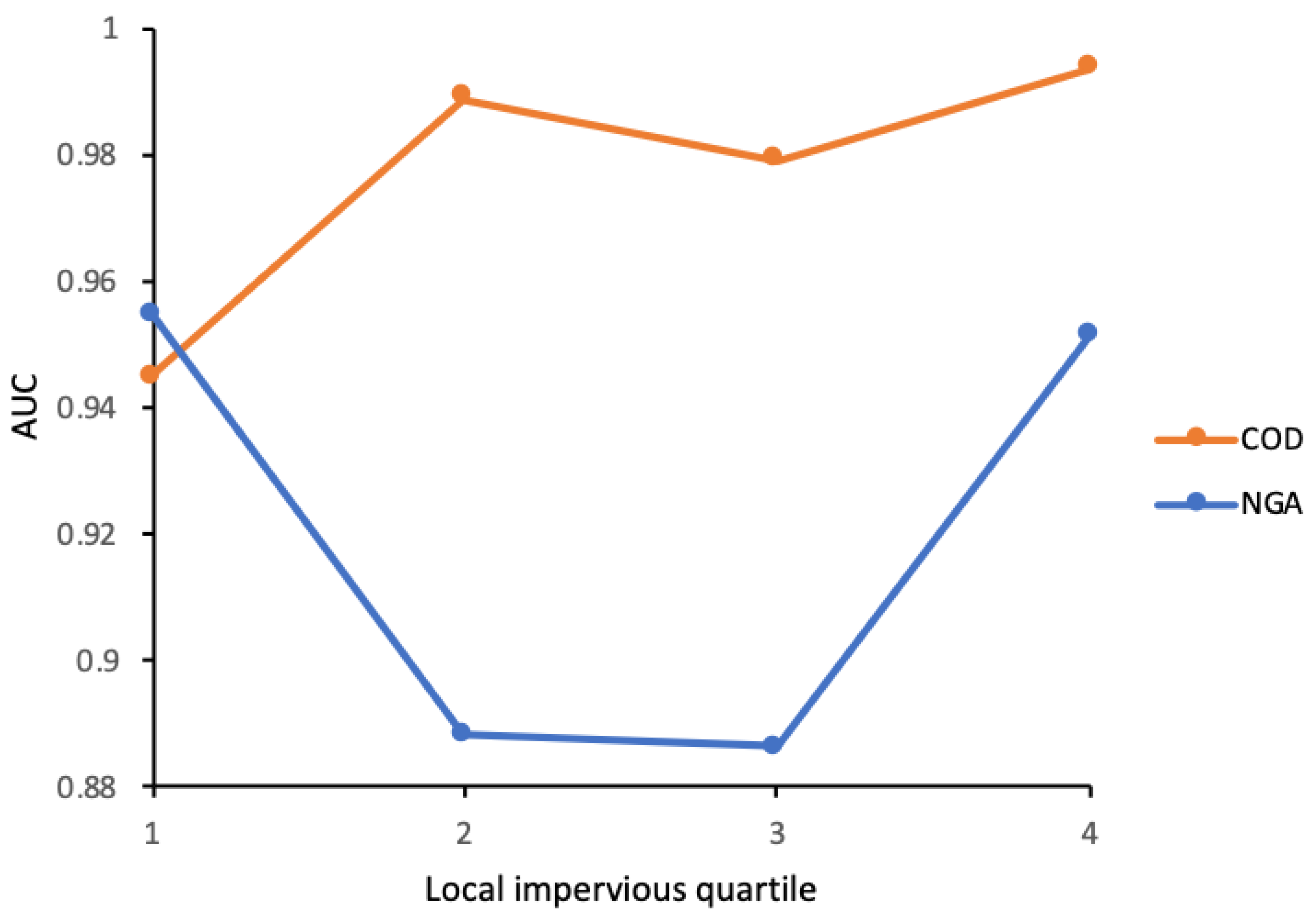
4.1. Sensitivity Testing of Window Generalization Method
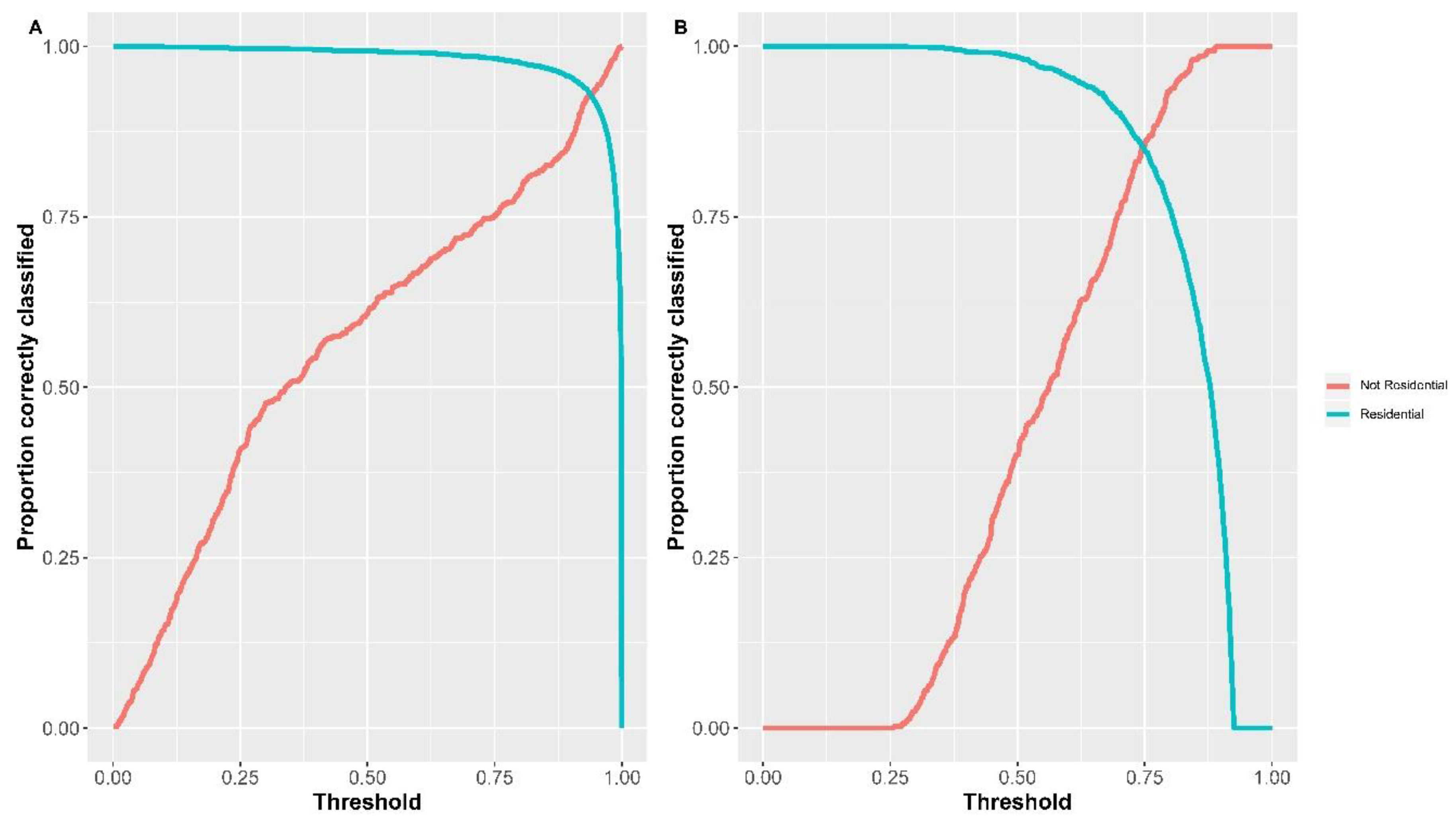
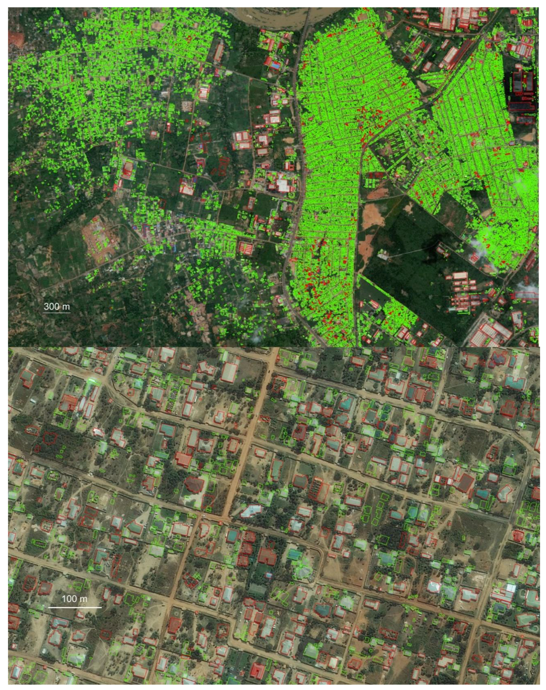
A window generalisation method was utilised in the GIS workflow in order to assist in the attribution of non-OSM residential building labels to building polygons. The authors know of no other examples of studies that use average moving windows in such workflow in order to produce datasets for input to binary building classification models. For this reason, some sensitivity testing was undertaken as to the effect that use of different window sizes (or none) have upon visualised building classifications as output from the superlearner model. Testing assesses (via human operator) whether window generalisation introduces discernible misclassifications into modelled output, when compared to satellite imagery and place labels derived from web mapping services. During testing, all workflow and model parameters are kept constant except for window size. A base case is also considered in which no window averaging is used. In that base case, a single non-OSM residential building label is attributed to each building polygon, only where at least one building label is found to be contained within the polygon. More substantial testing of a quantitative nature is not undertaken because there is insufficient label data available to this study with which to create a suitably sized subset of the data used during the actual window sampling or modelling. Were a greater amount of suitable data available then quantitative testing could provide a useful numerical performance indicator as to the effect of each different window size upon a test set containing known building label values. In the future, implementation of a form of quantitative sensitivity testing can be examined when enough new label data become available.
In sensitivity testing we do not explore the use of window sizes larger than that considered necessary to generalise the positioning of labels in line with the estimated maximum margin of error of label positions during field survey (i.e., a 5 × 5 cell square window of total size ≈450 m at the Equator, the chosen window size). This is because as window size increases, greater numbers of buildings become classified as residential. This has the effect of inflating the AUC value of a building classification model. Our window generalisation method mitigates against these issues because non-OSM residential zones (from which coincident building footprints are assigned residential attributes) are created using a cautious approach (see Method section). The approach strictly limits zone coverage to where there is a high level of certainty that building footprints will be residential.
The sensitivity testing indicates that smaller window sizes produce classification ‘banding’ (i.e., zones of misclassified buildings, most likely attributable to insufficient averaging of non-OSM label positions) in the visualised output for both COD and NGA. Such banding is not present when the chosen window size is used, nor in the base case. As is to be expected, model statistical output from the sensitivity tests show a slight increase in AUC values for both COD and NGA as window size increases from a 3 × 3 cell square window of total 10 m size at the Equator. This increase is largest when AUC at the chosen window size is compared to AUC in the base case (though modest at 0.02 and 0.8 for COD and NGA, respectively).
The sensitivity testing reveals that the use of window generalisation is of value in providing confidence in label attribution to residential buildings, with the caveat that it introduces a further variable to the method—that of the window size at which the analysis takes place. Whilst testing indicated that the window generalisation method (at chosen window size) provides best visualised output, and that the effect on AUC is minimal, nevertheless, both the window and ‘windowless’ (i.e., base case) methods may be considered of value depending on the use case and available label data (and estimated positional error of these). Indeed, the argument can be made that both methods identify regions of confidence in label attribution to residential buildings, because in urban locations such buildings typically cluster (i.e., Tobler’s First Law, which states that things that are closer together share more similarities than things that are further apart). Residential or nonresidential buildings typically cluster because of urban planning (and potentially other sociospatial processes). Whether window generalisation is used to average residential labels into a grid and matched to buildings, or whether specific labels are matched to specific buildings by spatial coincidence alone, such clustering will be identified. Future work could further explore the effect that variation in window size has on modelled predictions, especially when other parameters (predictor variables) of the model are altered. This could include the use of different window sizes according to the density of buildings, or instead assign labels to the closest ‘n’ number of buildings within a radius.

4.2. Model Output

The statistical outputs of the building classification model are at national level (apart from local imperviousness by quantile, which focuses on model performance in locations of differing urbanicity). This is in order to draw direct comparisons with the model output of Sturrock et al. [18]. We do not address statistical output from the model at regional or city level. This is due to insufficient sample sizes to make such comparisons useful, or sometimes even possible—a problem that is particularly acute in the case of Nigeria. With more data, interesting results might be obtained by training the model in one region/city and predicting on another within the same country. This would be useful to show the transferability of the model. Future research should therefore develop this aspect of the work as more building label data become available. Additionally, some of the predictor variables that are used in the model incorporate geographical proximity effects into the modelling process. These might help to mitigate against bias in predictions caused by spatial autocorrelation in the data (which is often ignored in random forest and similar machine learning modelling processes). However, the effect of these variables cannot be quantified without the examination of spatial autocorrelation in the residuals. Exploration of the effect of such variables upon spatial autocorrelation will make an interesting addition to future work as the model is developed.
With reference to Figure 3, there is a clear increase in building classification model performance with increasing urbanicity in COD (0.945 to 0.993 AUC). As in the Sturrock et al. [18] Swaziland (SWZ) example, this increase in performance may be due to differences in the characteristics of buildings in very urban areas in COD relative to those in very urban areas within NGA, or relative to the same in the Botswana (BWA) example of Sturrock et al. [18]. The increase in performance is less likely to be due to the amount of training data available with which to inform the model (Table 2). This is because there are significantly more training data available for COD than is the case for either SWZ or BWA. Either way, the AUC value for the COD model is extremely high at 0.98, performing better than the SWZ and the BWA cases (AUC of 0.95 and 0.96, respectively). For NGA, model performance peaks in least urban and very urban areas (Figure 3. 0.955 and 0.951 AUC, respectively). This makes sense because in such areas the built environment should be more homogenous and so easier for the model to predict. This is similar behaviour to the BWA case. Whilst the AUC value for the NGA model is very high at 0.93, the slightly lower performance relative to that for BWA may be due to the still limited availability of building label data with which to train the NGA model (Table 2). Additionally, the difference could be due to greater heterogeneity in the built environment of NGA than is the case in BWA, SWZ, or COD. Nevertheless, both COD and NGA show very good discriminatory performance regardless of setting.
The statistical results demonstrate that building classification model performance (AUC) is robust when a variety of input footprint datasets are utilised for different low and middle income countries in which building label data are relatively scarce. Additionally, they show that use of more complete input datasets can considerably improve model performance over that possible when only OSM footprint and attribute data are utilised (e.g., Sturrock et al. [18]). The additional data used for Nigeria makes the country modellable using this method, when previously it would not have been due to lack of data. However, comparison of the source satellite imagery to the classified building footprints (DigitizeAfrica data © 2020 Maxar Technologies, Ecopia.AI) by a human operator demonstrates that further improvements in model performance are required if the model is to near perfectly discriminate between residential/nonresidential classifications in visualised output (i.e., real world performance). We additionally employed place labels derived from web mapping services in our comparison. Classification performance of the model is generally effective at ‘neighbourhood’ scale. Figure 5, top, shows an example of this—residential and nonresidential clusters of buildings appear well defined, with the assessment by the model of building size, shape, and proximity to nearest neighbouring building apparently highly effective. The predictor variables mentioned are just some of those used by the model but can perhaps be considered the most intuitive. However, in suburban localities, at ‘street’ scale, it is apparent that buildings can sometimes be misclassified. Figure 5, bottom, shows a predominantly residential area [46] that has many buildings classified as nonresidential. Such apparent building misclassification might be due to unusual heterogeneity of building structures in the given locality when compared to urban areas in the country at large, and/or due to limited training data within the locality. Certainly, additional building label data will be required in the future in order to train the model more effectively. Future work should also enhance the visualised performance of the model by developing and expanding upon the predictor variables used within. This might include finding a way to better discriminate building classification within suburban locations.
There are limitations and opportunities for future research in addition to those already mentioned. There may be some error in OSM or other label dataset attributes, or bias could be introduced if building type information is only available for certain categories of structures, such as for retail outlets. Whilst the building label data used in this study somewhat address the need flagged by Sturrock et al. [18] to use ground truthed data as part of that input to the building classification model, nevertheless, dataset completeness and attribute accuracy will never be perfect. The modelled problem was a simple binary one, limiting usefulness of the data to other fields. The intention is to address this in the future by broadening modelled categories to include mixed use, informal, and other types of buildings.
It might be possible to experiment with training and testing of the building classification model using highest quality building footprint and label data available for high income countries. This would be the case only where urban areas are identified as potentially analogous (in terms of settlement layout, area, and population size) to those in particular low and middle income settings. In theory, better completeness and accuracy of data in training allows higher quality predictions to be made, with the proviso that urban areas in the training and prediction datasets must be of similar character.

5. Conclusions

In this paper we developed a novel GIS workflow that semiautomates the preparation of data for input to a recently developed, stacked generalisation, ensemble, building classification model. Building footprint data are becoming more commonly available due to image extraction methods. However, use of such data are somewhat limited by a lack of labels. Other data sources can effectively label structures (during fieldwork or surveys), and our workflow fuses these disparate sources to inform the predictive model. The workflow is designed to be particularly useful to those who apply the building classification model to further countries, and to those who input separate building footprint and label (as well as impervious surface) data from diverse sources, especially as new data become available. For the first time, the model was applied to urban areas in the Democratic Republic of the Congo (COD), and Nigeria (NGA), using footprint and building attribute datasets of greater coverage, completeness, and attribute consistency than previously available. The classification model predicts whether buildings are residential or nonresidential within each country. The statistical results show that the ensemble model correctly classifies between 85% and 93% of structures as residential and nonresidential across both countries. This is an improvement on previous research [18] that used less complete datasets as input to the same model, applied to similar and proximal low and middle income settings. For COD, outputs show better discrimination between residential and nonresidential buildings than found possible for case studies in the previous study. For NGA, the newly available source datasets provide sufficient training and test data to make the country modellable for the first time using the Sturrock et al. model [18], with good results. The classified model outputs will be particularly useful in informing models of human population. This, in turn, will allow improved population models to be produced that will better inform a range of related applications including urban planning, resource allocation, and service delivery.
Future development of the building classification model will involve the modification and expansion of the classification algorithm to include a greater range of appropriate data inputs and predictor variables in order to improve predictive power in low and middle income settings. These inputs might include data pertaining to the height of buildings, patch density of urban form [14], or discrimination of building roof top types via use of multispectral imagery. Further, we aim to enhance the completeness and attribute consistency of data input to the model via the acquisition of additional or improved data as these become available. Future work should also explore model transferability at regional/city level, the effect of particular predictor variables upon spatial autocorrelation in the data, and the effect that variation in window size has on building labels and modelled predictions. Acquisition of training data for urban areas in high income countries that are analogous to urban areas in low and middle income settings should be investigated in order to improve model predictions if possible. Finally, our intention is to adapt the model in order to classify a wider variety of building function. Rather than a simple binary residential/nonresidential classification, the model should be expanded to include classifications of mixed use and informal settlements, in order to better inform population models.

Supplementary Materials

The following are available online at https://0-www-mdpi-com.brum.beds.ac.uk/2072-4292/12/23/3847/s1, Supplementary Information, Figure S1, CV-AUC values obtained from each of the base learners and superlearner plotted in decreasing value of AUC for the Democratic Republic of the Congo and Nigeria, Table S1, Coefficients estimated by the superlearner algorithm for each base learner. And at https://0-www-mdpi-com.brum.beds.ac.uk/2072-4292/12/23/3847/s2, Workflow Code.

Author Contributions

Conceptualization, C.T.L., H.J.W.S., A.J.T. and W.C.J.; Methodology, C.T.L., H.J.W.S. and D.R.L.; Software, C.T.L. and H.J.W.S.; Validation, C.T.L.; Formal Analysis, C.T.L.; Investigation, C.T.L.; Resources, H.J.W.S.; Data Curation, C.T.L.; Writing—Original Draft Preparation, C.T.L.; Writing—Review and Editing, C.T.L., H.J.W.S., D.R.L., W.C.J., A.N.L. and A.J.T.; Visualisation, C.T.L.; Supervision, A.J.T., A.N.L. and H.J.W.S.; Project Administration, C.T.L.; Funding Acquisition, A.J.T. All authors have read and agreed to the published version of the manuscript.

Funding

This work is part of the GRID3 project (Geo-Referenced Infrastructure and Demographic Data for Development), funded by the Bill and Melinda Gates Foundation and the United Kingdom Foreign, Commonwealth and Development Office (#OPP1182408). Project partners include the United Nations Population Fund (UNFPA), Center for International Earth Science Information Network (CIESIN) in the Earth Institute at Columbia University, and the Flowminder Foundation.

Acknowledgments

The authors acknowledge the use of building footprint and highway data provided by OpenStreetMap (© 2020 OpenStreetMap contributors; geofabrik.de); building footprint data provided by Maxar Technologies (DigitizeAfrica data © 2020 Maxar Technologies, Ecopia.AI); building label data for Kinshasa and North Ubangi, COD, provided by the World Bank (World Bank Group, 2018); impervious surface data provided by US NASA (SEDAC) (Brown de Colstoun et al., 2017). The University of California, Los Angeles (UCLA)-Democratic Republic of the Congo (DRC) Health Research and Training Program, the Kinshasa School of Public Health (KSPH), and the Bureau Central du Recensement (BCR) coordinated and conducted the two household survey rounds in COD during 2017–2018. The Oak Ridge National Laboratory (ORNL) contributed to the first round of household survey. ORNL designed, and eHealth Africa implemented, the collection of household survey data in NGA during 2016–17. WorldPop (University of Southampton) designed, and eHealth Africa implemented, the collection of household survey data in NGA during 2018–2019. The authors acknowledge the use of the IRIDIS High Performance Computing Facility, and associated support services at the University of Southampton, in the completion of this work. We also acknowledge the help of the WorldPop Population Modelling Team for critique of the GIS workflow discussed in this paper, as well as project partners and Heather R. Chamberlain at WorldPop for liaison with Maxar and the Bill and Melinda Gates Foundation regarding acquirement of data.

Conflicts of Interest

The authors declare no conflict of interest.

References

  1. World Health Organization & United Nations. Human Settlements Programme. Hidden Cities: Unmask. and Overcoming Health Inequities in Urban Settings; World Health Organization: Geneva, Switzerland, 2010; p. 126. [Google Scholar]
  2. UN Habitat. World Cities Report 2016: Urbanization and Development—Emerging Futures; United Nations Human Settlements Programme (UN-Habitat): Nairobi, Kenya, 2016; p. 262. [Google Scholar]
  3. United Nations. New Urban Agenda; United Nations: New York, NY, USA, 2017. [Google Scholar]
  4. Wardrop, N.A.; Jochem, W.C.; Bird, T.J.; Chamberlain, H.R.; Clarke, D.; Kerr, D.; Bengtsson, L.; Juran, S.; Seaman, V.; Tatem, A.J. Spatially disaggregated population estimates in the absence of national population and housing census data. Proc. Natl. Acad. Sci. USA 2018, 115, 3529–3537. [Google Scholar] [CrossRef] [Green Version]
  5. Nieves, J.J.; Stevens, F.R.; Gaughan, A.E.; Linard, C.; Sorichetta, A.; Hornby, G.; Patel, N.N.; Tatem, A.J. Examining the correlates and drivers of human population distributions across low- and middle-income countries. J. R. Soc. Interface 2017, 14, 20170401. [Google Scholar] [CrossRef] [PubMed] [Green Version]
  6. Reed, F.; Gaughan, A.E.; Stevens, F.R.; Yetman, G.; Sorichetta, A.; Tatem, A.J. Gridded Population Maps Informed by Different Built Settlement Products. Data 2018, 3, 33. [Google Scholar] [CrossRef] [Green Version]
  7. Stevens, F.R.; Gaughan, A.E.; Nieves, J.J.; King, A.; Sorichetta, A.; Linard, C.; Tatem, A.J. Comparisons of two global built area land cover datasets in methods to disaggregate human population in eleven countries from the global South. Int. J. Dig. Earth 2019, 13, 78–100. [Google Scholar] [CrossRef]
  8. Jochem, W.C.; Bird, T.J.; Tatem, A.J. Identifying residential neighbourhood types from settlement points in a machine learning approach. Comput. Environ. Urban Syst. 2018, 69, 104–113. [Google Scholar] [CrossRef]
  9. Hecht, R.; Meinel, G.; Buchroithner, M. Automatic identification of building types based on topographic databases—A comparison of different data sources. Int. J. Cart. 2015, 1, 18–31. [Google Scholar] [CrossRef] [Green Version]
  10. Barr, S.L.; Barnsley, M.J.; Steel, A. On the separability of urban land-use categories in fine spatial scale land-cover data using structural pattern recognition. Environ. Plan B Plan Design 2004, 31, 397–418. [Google Scholar] [CrossRef]
  11. Steiniger, S.; Lange, T.; Burghardt, D.; Weibel, R. An Approach for the Classification of Urban Building Structures Based on Discriminant Analysis Techniques. Trans. GIS 2008, 12, 31–59. [Google Scholar] [CrossRef]
  12. Lüscher, P.; Weibel, R. Exploiting empirical knowledge for automatic delineation of city centres from large-scale topographic databases. Comput. Environ. Urban Syst. 2013, 37, 18–34. [Google Scholar] [CrossRef] [Green Version]
  13. He, X.; Zhang, X.; Xin, Q. Recognition of building group patterns in topographic maps based on graph partitioning and random forest. ISPRS J. Photogram. Remote Sens. 2018, 136, 26–40. [Google Scholar] [CrossRef]
  14. Jochem, W.C.; Leasure, D.R.; Pannell, O.; Chamberlain, H.R.; Jones, P.; Tatem, A.J. Classifying settlement types from multi-scale spatial patterns of building footprints. Environ. Plan B Urban Analyt. City. Sci. 2020. [Google Scholar] [CrossRef]
  15. Longley, P.A.; Mesev, V. On the Measurement and Generalisation of Urban Form. Environ. Plan A Econ. Space 2016, 32, 473–488. [Google Scholar] [CrossRef]
  16. Mesev, V. Identification and characterisation of urban building patterns using IKONOS imagery and point-based postal data. Comput. Environ. Urban Syst. 2005, 29, 541–557. [Google Scholar] [CrossRef]
  17. Mesev, V. Fusion of point-based postal data with IKONOS imagery. Inf. Fusion. 2007, 8, 157–167. [Google Scholar] [CrossRef]
  18. Sturrock, H.J.W.; Woolheater, K.; Bennett, A.F.; Andrade-Pacheco, R.; Midekisa, A. Predicting residential structures from open source remotely enumerated data using machine learning. PLoS ONE 2018, 13, e0204399. [Google Scholar] [CrossRef] [PubMed] [Green Version]
  19. Wolpert, D.H. Stacked generalization. Neural Networks 1992, 5, 241–259. [Google Scholar] [CrossRef]
  20. Lu, Z.; Im, J.; Rhee, J.; Hodgson, M. Building type classification using spatial and landscape attributes derived from LiDAR remote sensing data. Landsc. Urban Plan 2014, 130, 134–148. [Google Scholar] [CrossRef]
  21. Xie, J.; Zhou, J. Classification of Urban Building Type from High Spatial Resolution Remote Sensing Imagery Using Extended MRS and Soft BP Network. IEEE J. Sel. Top. Appl. Earth Obs. Remote Sens. 2017, 10, 3515–3528. [Google Scholar] [CrossRef]
  22. Midekisa, A.; Holl, F.; Savory, D.J.; Andrade-Pacheco, R.; Gething, P.W.; Bennett, A.; Sturrock, H.J.W. Mapping land cover change over continental Africa using Landsat and Google Earth Engine cloud computing. PLoS ONE 2017, 12, e0184926. [Google Scholar] [CrossRef]
  23. World Bank Group. The World Bank Data Catalog, DRC—Building points for Kinshasa and North Ubangi. Available online: https://datacatalog.worldbank.org/dataset/building-points-kinshasa-and-north-ubangi (accessed on 21 August 2020).
  24. Oak Ridge National Laboratory (ORNL). Nigeria Household Surveys in 2016 and 2017; Bill & Melinda Gates Foundation: Seattle, WA, USA, 2018. [Google Scholar]
  25. eHealth Africa and WorldPop (University of Southampton). Nigeria Household Surveys in 2018 and 2019; Bill & Melinda Gates Foundation: Seattle, WA, USA, 2019. [Google Scholar]
  26. University of California - Los Angeles (UCLA) and Kinshasa School of Public Health (KSPH). Kinshasa, Kongo Central and Former Bandundu Household Surveys in 2017 and 2018; University of California: Los Angeles, CA, USA, 2018. [Google Scholar]
  27. Brown de Colstoun, E.C.; Huang, C.; Wang, P.; Tilton, J.C.; Tan, B.; Phillips, J.; Niemczura, S.; Ling, P.-Y.; Wolfe, R.E. Global Man-Made Impervious Surface (GMIS) Dataset From Landsat; NASA Socioeconomic Data and Applications Center (SEDAC): Palisades, NY, USA, 2017. [Google Scholar] [CrossRef]
  28. Maxar Technologies. Building Footprints. Available online: https://www.digitalglobe.com/products/building-footprints?utm_source=website&utm_medium=blog&utm_campaign=Building-Footprints (accessed on 21 August 2020).
  29. Ecopia and DigitalGlobe. Technical Specification: Ecopia Building Footprints Powered by DigitalGlobe. Available online: https://dg-cms-uploads-production.s3.amazonaws.com/uploads/legal_document/file/109/DigitalGlobe_Ecopia_Building_Footprints_Technical_Specification.pdf (accessed on 21 August 2020).
  30. Haklay, M.; Basiouka, S.; Antoniou, V.; Ather, A. How Many Volunteers Does it Take to Map an Area Well? The Validity of Linus’ Law to Volunteered Geographic Information. Carto J. 2013, 47, 315–322. [Google Scholar] [CrossRef] [Green Version]
  31. Lloyd, C.T.; Sorichetta, A.; Tatem, A.J. High resolution global gridded data for use in population studies. Sci. Data 2017, 4, 170001. [Google Scholar] [CrossRef] [PubMed] [Green Version]
  32. Brown de Colstoun, E.C.; Huang, C.; Wang, P.; Tilton, J.C.; Tan, B.; Phillips, J.; Niemczura, S.; Ling, P.-Y.; Wolfe, R.E. Documentation for Global Man-made Impervious Surface (GMIS) Dataset From Landsat, v1 (2010); NASA Socioeconomic Data and Applications Center (SEDAC): Palisades, NY, USA, 2017. [Google Scholar] [CrossRef]
  33. Gutman, G.; Huang, C.; Chander, G.; Noojipady, P.; Masek, J.G. Assessment of the NASA–USGS Global Land Survey (GLS) datasets. Remote Sens. Environ. 2013, 134, 249–265. [Google Scholar] [CrossRef]
  34. Polley, E.; LeDell, E.; Kennedy, C.; Lendle, S.; van der Laan, M. R Package ‘SuperLearner’ Documentation. Available online: https://cran.r-project.org/web/packages/SuperLearner/SuperLearner.pdf (accessed on 21 August 2020).
  35. R Core Team. R: A Language and Environment for Statistical Computing. Available online: https://www.r-project.org/ (accessed on 21 August 2020).
  36. van der Laan, M.J.; Polley, E.C.; Hubbard, A.E. Super learner. Stat. Appl. Genet. Mol. Biol. 2007, 6. [Google Scholar] [CrossRef] [PubMed]
  37. Breiman, L. Random Forests. Mach. Learn. 2001, 45, 5–32. [Google Scholar] [CrossRef] [Green Version]
  38. Friedman, J.H. Greedy function approximation: A gradient boosting machine. Annal. Stat. 2001, 29, 1189–1232. [Google Scholar] [CrossRef]
  39. DeLong, E.R.; DeLong, D.M.; Clarke-Pearson, D.L. Comparing the areas under two or more correlated receiver operating characteristic curves: A nonparametric approach. Biometrics 1988, 44, 837–845. [Google Scholar] [CrossRef]
  40. Robin, X. ROC.test - Compare The AUC Of Two ROC Curves. From pROC v1.16.2. Available online: https://www.rdocumentation.org/packages/pROC/versions/1.16.2/topics/roc.test (accessed on 9 November 2020).
  41. Robin, X.; Turck, N.; Hainard, A.; Tiberti, N.; Lisacek, F.; Sanchez, J.C.; Muller, M. pROC: An open-source package for R and S+ to analyze and compare ROC curves. BMC Bioinform. 2011, 12, 77. [Google Scholar] [CrossRef]
  42. Sturrock, H.J.W. OSM Building Prediction Repository. Available online: https://github.com/disarm-platform/OSM_building_prediction (accessed on 21 August 2020).
  43. Bruy, A.; Dubinin, M. Python Script for Extracting Values of Image According to the Point Shapefile. Available online: https://github.com/nextgis/extract_values/blob/master/extract_values.py (accessed on 21 August 2020).
  44. Stackoverflow.com. Limit Python Script RAM Usage in Windows. Available online: https://stackoverflow.com/questions/54949110/limit-python-script-ram-usage-in-windows (accessed on 21 August 2020).
  45. Perry, M. Zonal Statistics Vector-Raster Analysis. Available online: https://gist.github.com/perrygeo/5667173 (accessed on 21 August 2020).
  46. Google Maps. -11.6486225,27.4351423. Available online: https://www.google.com/maps/@-11.6486225,27.4351423,834m/data=!3m1!1e3 (accessed on 21 August 2020).
Figure 1. Distribution of OpenStreetMap (OSM) and other building label data, in (A) the Democratic Republic of the Congo (break-out box shows city of Lubumbashi in greater detail, including road network) and (B) Nigeria (break-out box shows city of Kano). Green and red points represent residential and nonresidential structures respectively. Data are plotted with opaque colours, and thus darker colours indicate more buildings of the same type (UCLA and KSPH [26]; eHealth Africa and WorldPop (University of Southampton) [25]; ORNL [24]; World Bank Group [23]; © 2020 OpenStreetMap contributors).
Remotesensing 12 03847 g001
Figure 2. Flow diagram of GIS workflow, including how outputs integrate into the building classification model. Input datasets to the workflow are denoted in grey, with GIS workflow processes shown in blue. Inputs to the model are shown in green, and are depicted with blue outlines if also outputs from a GIS workflow process. The model is denoted in red, with model outputs and associated processes, respectively, shown in black with red outlines.
Remotesensing 12 03847 g002
Figure 3. AUC values of the final building classification superlearner model by local impervious (urbanicity) quantile (a higher quantile value is more urban), for the Democratic Republic of the Congo and Nigeria.
Remotesensing 12 03847 g003
Figure 4. Classification performance of the building classification superlearner model using different cut-off thresholds, for (A) the Democratic Republic of the Congo and (B) Nigeria.
Remotesensing 12 03847 g004
Figure 5. Visualisations of classified residential (depicted in green) and nonresidential (red) building footprints, (Top) South-western Kaduna, Nigeria (co-ordinate location 7.390E, 10.470N; scale 1:16,000). The classification performance of the building classification model is observed to be generally effective at ‘neighbourhood’ scale (see text). (Bottom) North-western Lubumbashi, the Democratic Republic of the Congo (co-ordinate location 27.436E, 11.648S; scale 1:2700). A predominantly residential suburban locality at ‘street’ scale, demonstrating apparent building misclassifications (i.e., nonresidential) despite excellent statistical performance of the model (see text) (DigitizeAfrica data © 2020 Maxar Technologies, Ecopia.AI; © 2020 OpenStreetMap contributors).
Remotesensing 12 03847 g005
Table 1. Source datasets used as input to the building classification model, either via the GIS workflow or directly. Source datasets are here described. Data source, type, format, and spatial information are summarized.
NameSourceAcquisitionPublication YearData TypeSpatial ResolutionFormat/Pixel Type and DepthSpatial ReferenceSpatial Coverage
Maxar Technologies building footprintsDigitizeAfrica data. Maxar Technologies, Ecopia.AI2009–2019Late 2019/Early 2020Building footprints, vectorComparable to 1” (≈30 m)ESRI polygon shapefilesUTM WGS 1984National (COD and NGA)
OpenStreetMap (OSM) building footprintsOpenStreetMap contributors; geofabrik.deUp to Jan-20Jan-20Building footprints with building attribute labels, categorical vectorComparable to 1” (≈30 m)ESRI polygon shapefilesGCS WGS 1984National (COD and NGA)
OpenStreetMap (OSM) highwaysOpenStreetMap contributors; geofabrik.deUp to Jan-20Jan-20Highways, categorical vectorComparable to 1” (≈30 m)ESRI polyline shapefilesGCS WGS 1984National (COD and NGA)
Democratic Republic of the Congo (COD)—building points for Kinshasa and North UbangiThe World Bank Group [23]20182018Building attribute labels, categorical vectorComparable to 1” (≈30 m)ESRI point shapefilesGCS WGS 1984Kinshasa and North Ubangi provinces, COD
Nigeria (NGA)—household survey dataOak Ridge National Laboratory (ORNL) [24]2016–20172018Building attribute labels, categorical vector and tableComparable to 1” (≈30 m)ESRI point shapefiles/CSV tabularGCS WGS 1984Abia, Adamawa, Akwa Ibom, Bauchi, Ebonyi, Edo, Enugu, Gombe, Kaduna, Kebbi, Lagos, Ogun, Oyo, Sokoto, Yobe, and Zamfara states, NGA
eHealth Africa and WorldPop (University of Southampton) [25]2018–20192019
Democratic Republic of the Congo—household survey dataUniversity of California, Los Angeles (UCLA) and Kinshasa School of Public Health (KSPH) [26]2017–20182018Building attribute labels, categorical vector and tableComparable to 1” (≈30 m)ESRI point shapefiles/CSV tabularGCS WGS 1984Kinshasa, Kongo Central, Kwango, Kwilu, and Mai-Ndombe provinces, COD
Global Man-made Impervious Surface (GMIS) Dataset from Landsat, v1US NASA (SEDAC)/Center for International Earth Science Information Network (CIESIN), Columbia University [27]20102018Impervious surface (percentage per pixel), continuous raster1” (≈30 m)Geo-tiff/uint8GCS WGS 1984National (COD and NGA)
Table 2. Summary of structure data for the Democratic Republic of the Congo and Nigeria, used in building classification model training and testing.
Country Total with LabelsTotal without Labels
Democratic Republic of the Congo 98,2942,791,564
Residential93,794
Nonresidential4500
Nigeria 16,77611,476,015
Residential12,985
Nonresidential3791
Table 3. Performance of the building classification superlearner models when applied to the test data. The sensitivity (recall, or true positive rate) of the respective models for the two countries are shown in green, the specificity (true negative rate) in red. Classifications were made using the country specific cut-off threshold at which CV-classification accuracy was equal for residential and nonresidential structures.
Observed
Country NonresidentialResidential
Democratic Republic of the CongoPredictedNonresidential463753
Residential369668
% correctly classified92.892.8
NigeriaPredictedNonresidential360212
Residential611230
% correctly classified85.585.3
Publisher’s Note: MDPI stays neutral with regard to jurisdictional claims in published maps and institutional affiliations.

