Contextualizing the 2019–2020 Kangaroo Island Bushfires: Quantifying Landscape-Level Influences on Past Severity and Recovery with Landsat and Google Earth Engine


Abstract
:
1. Introduction
2. Materials and Methods
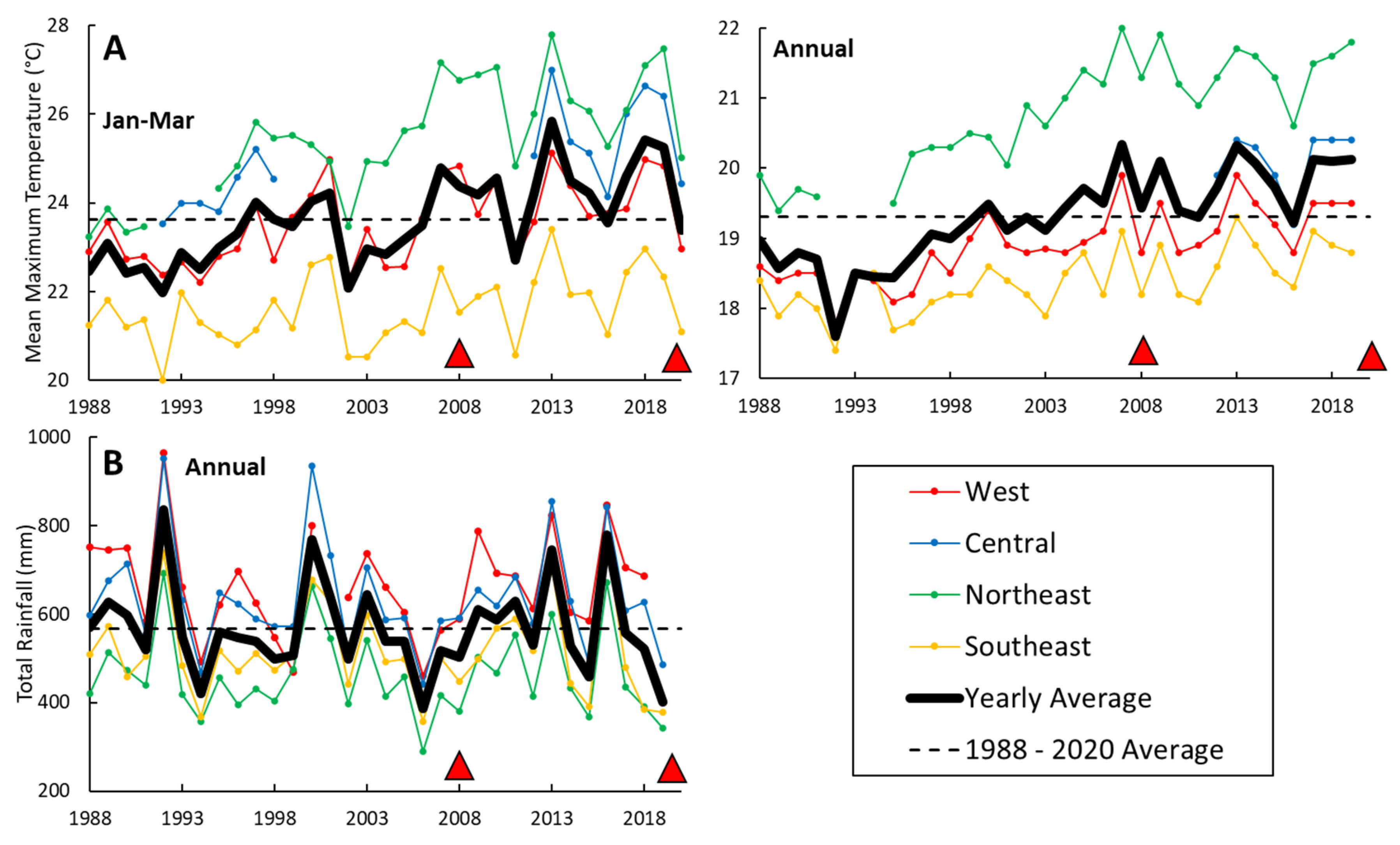
2.1. Study Area
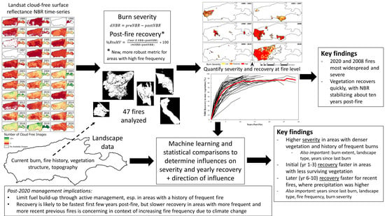
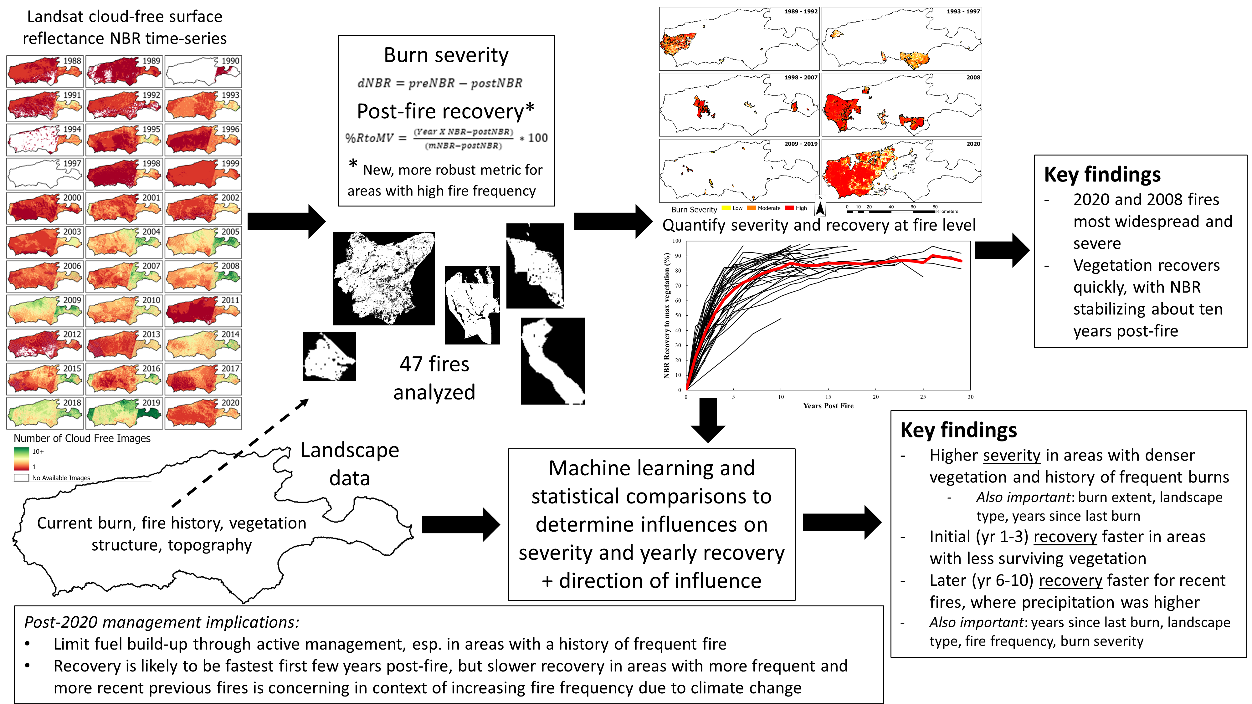
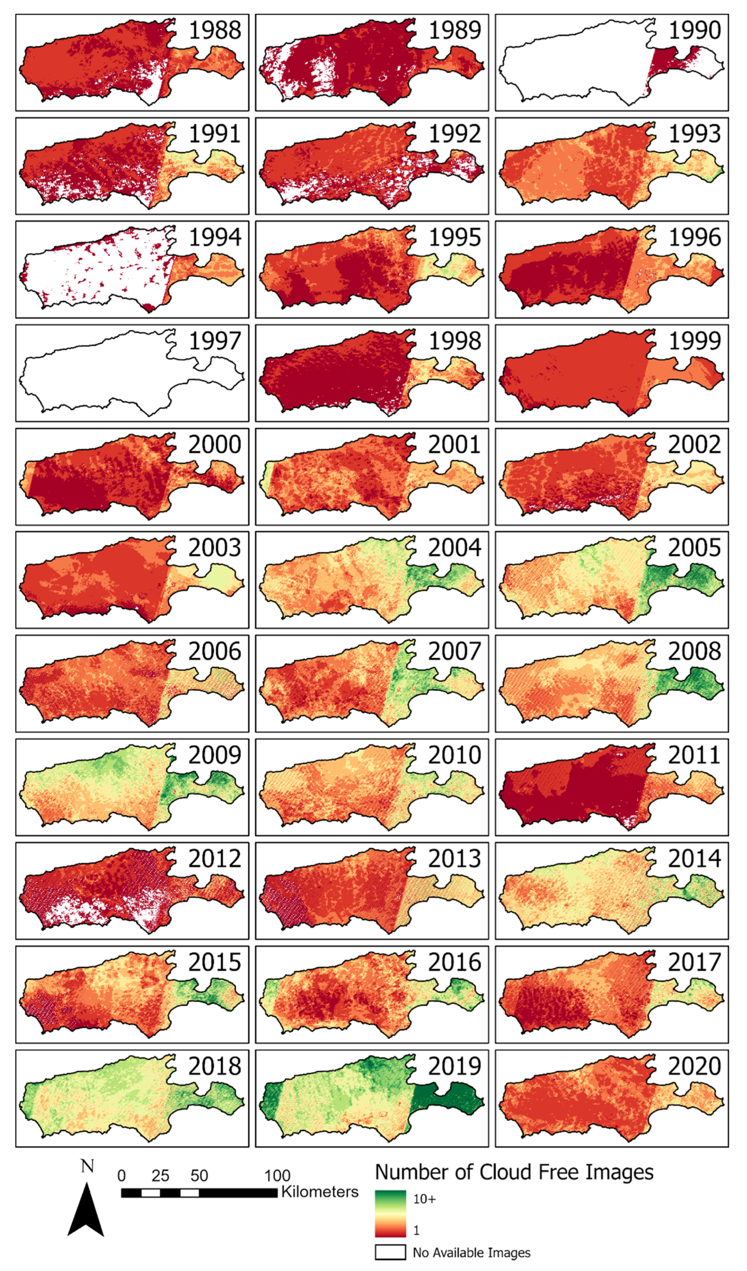
2.2. Building Landsat Fire History Time-Series
2.3. Assessing Landscape-Level Influences
3. Results
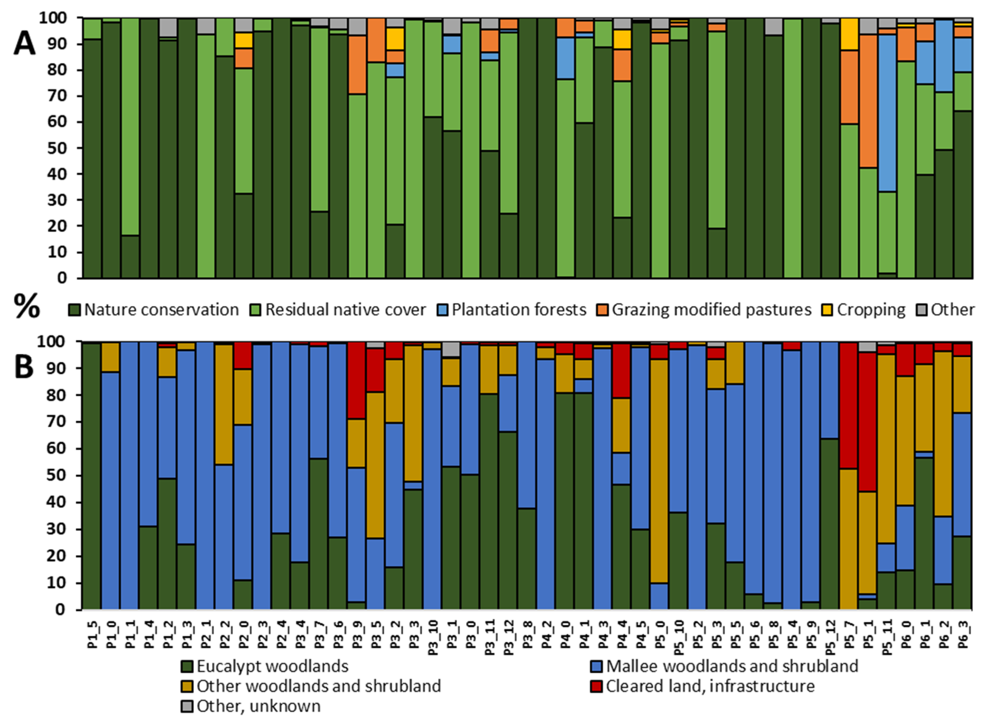
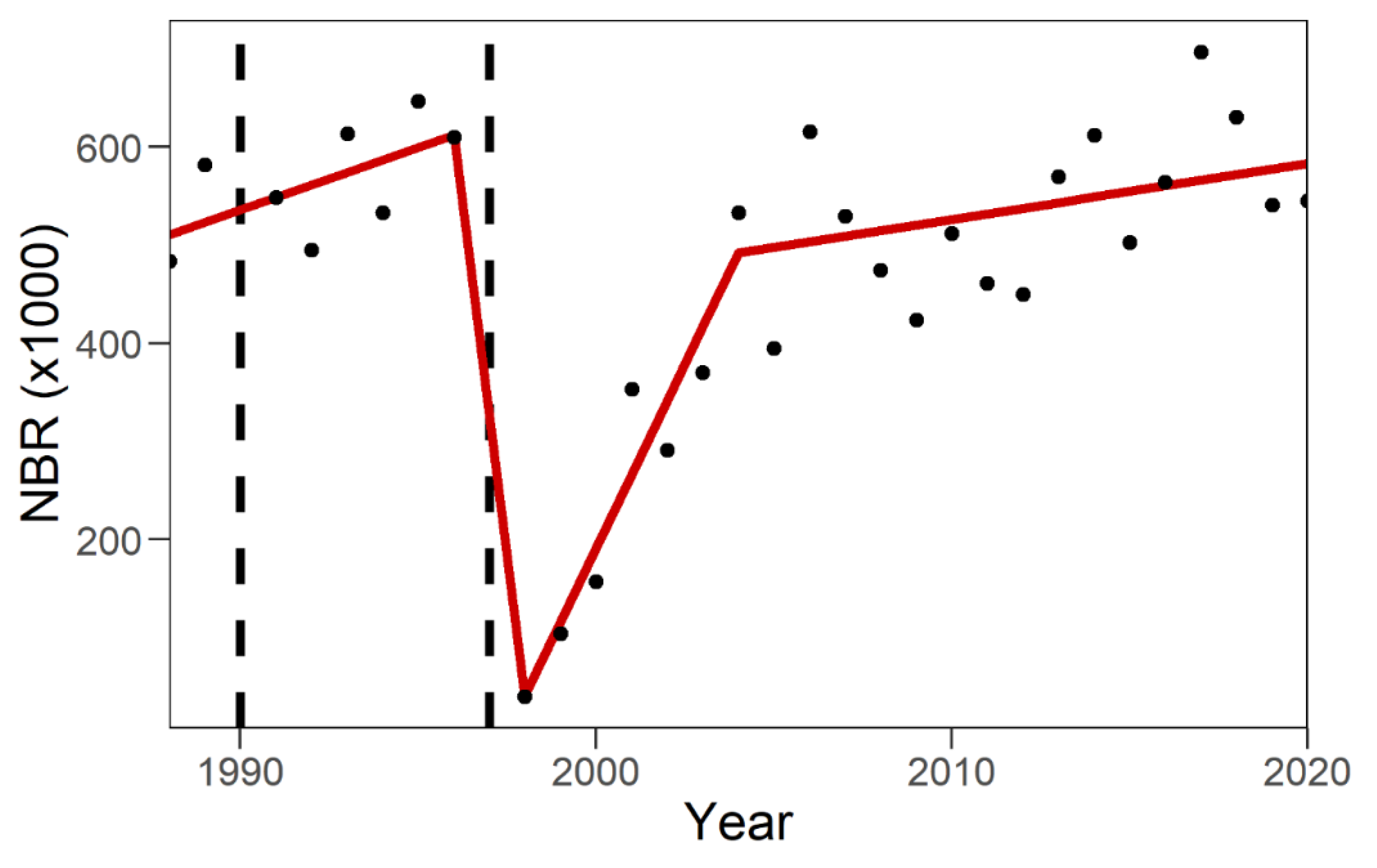
3.1. Fire History
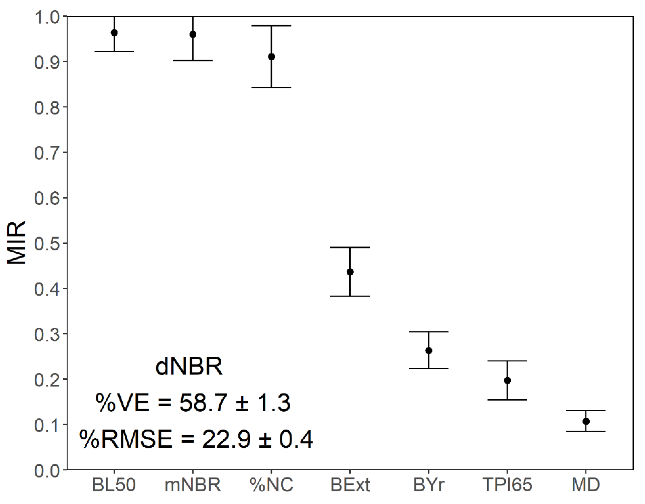
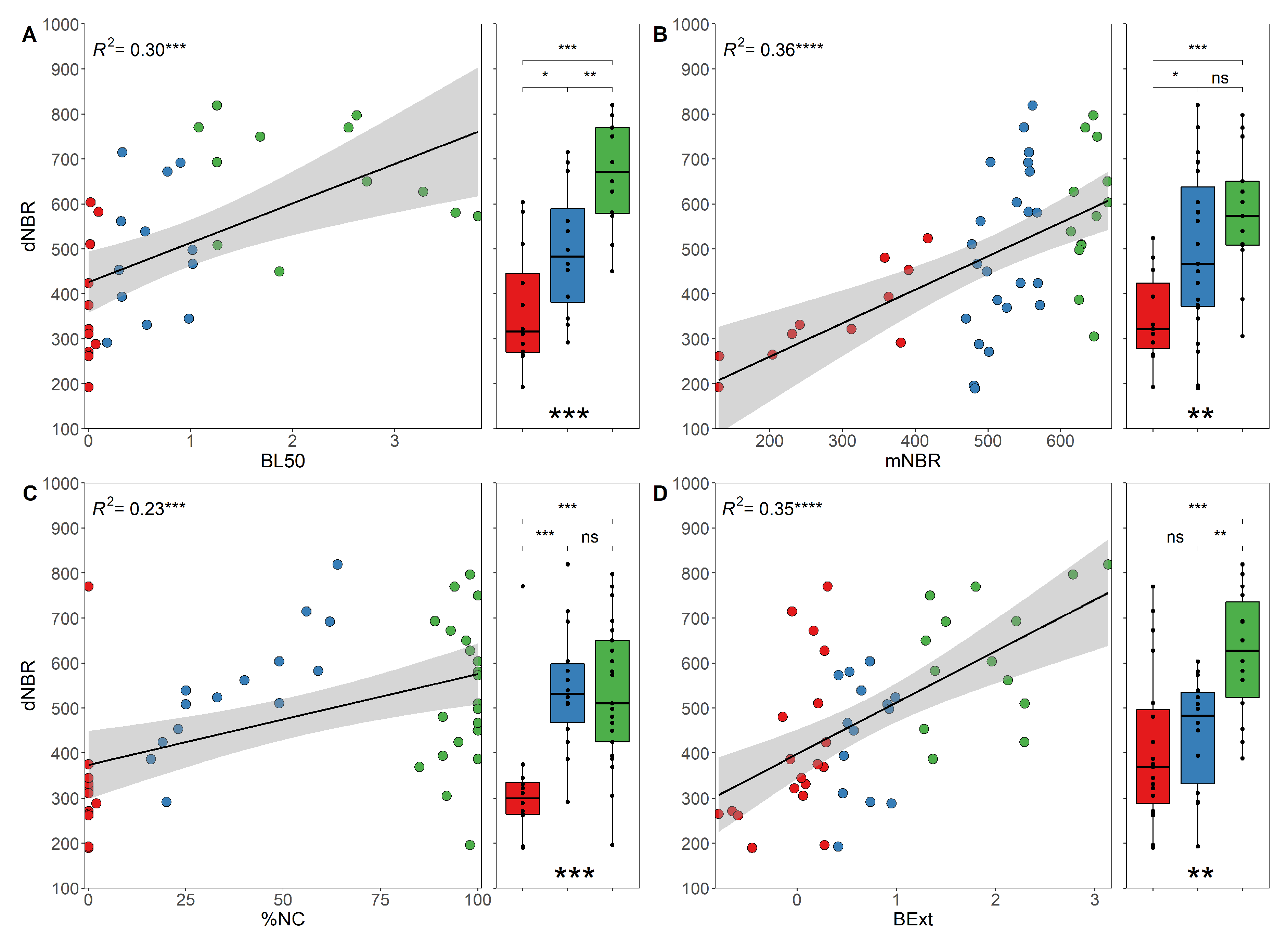
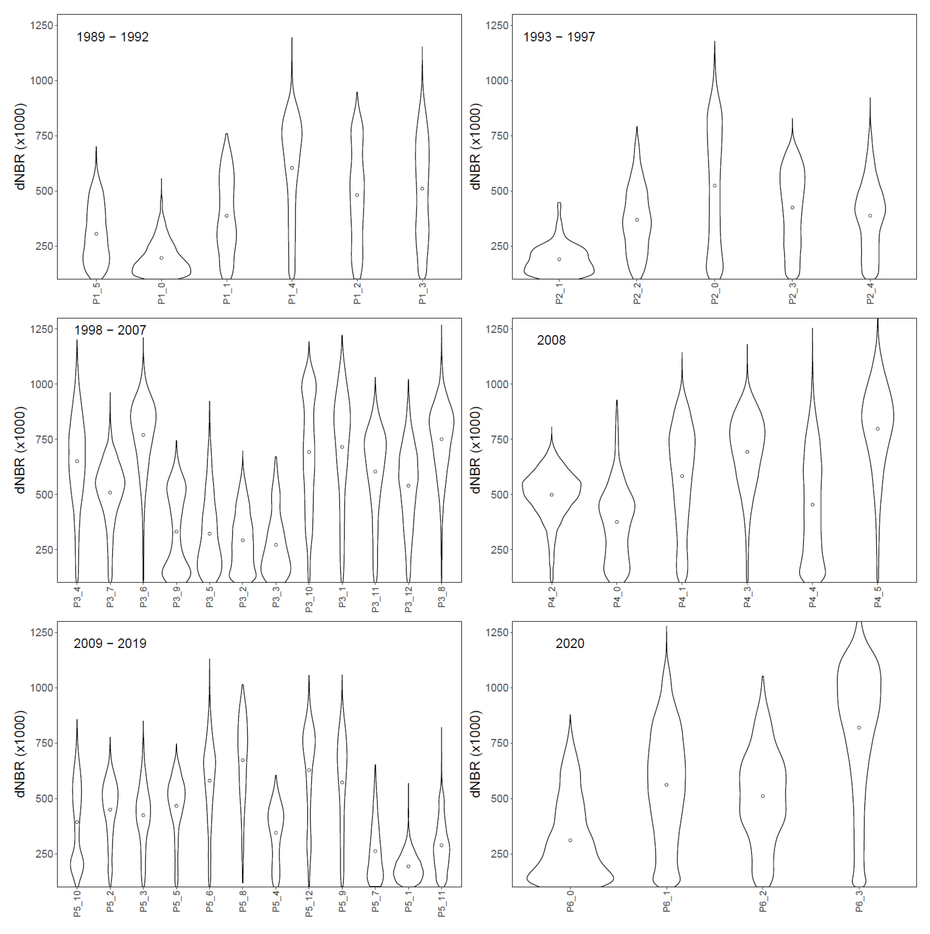
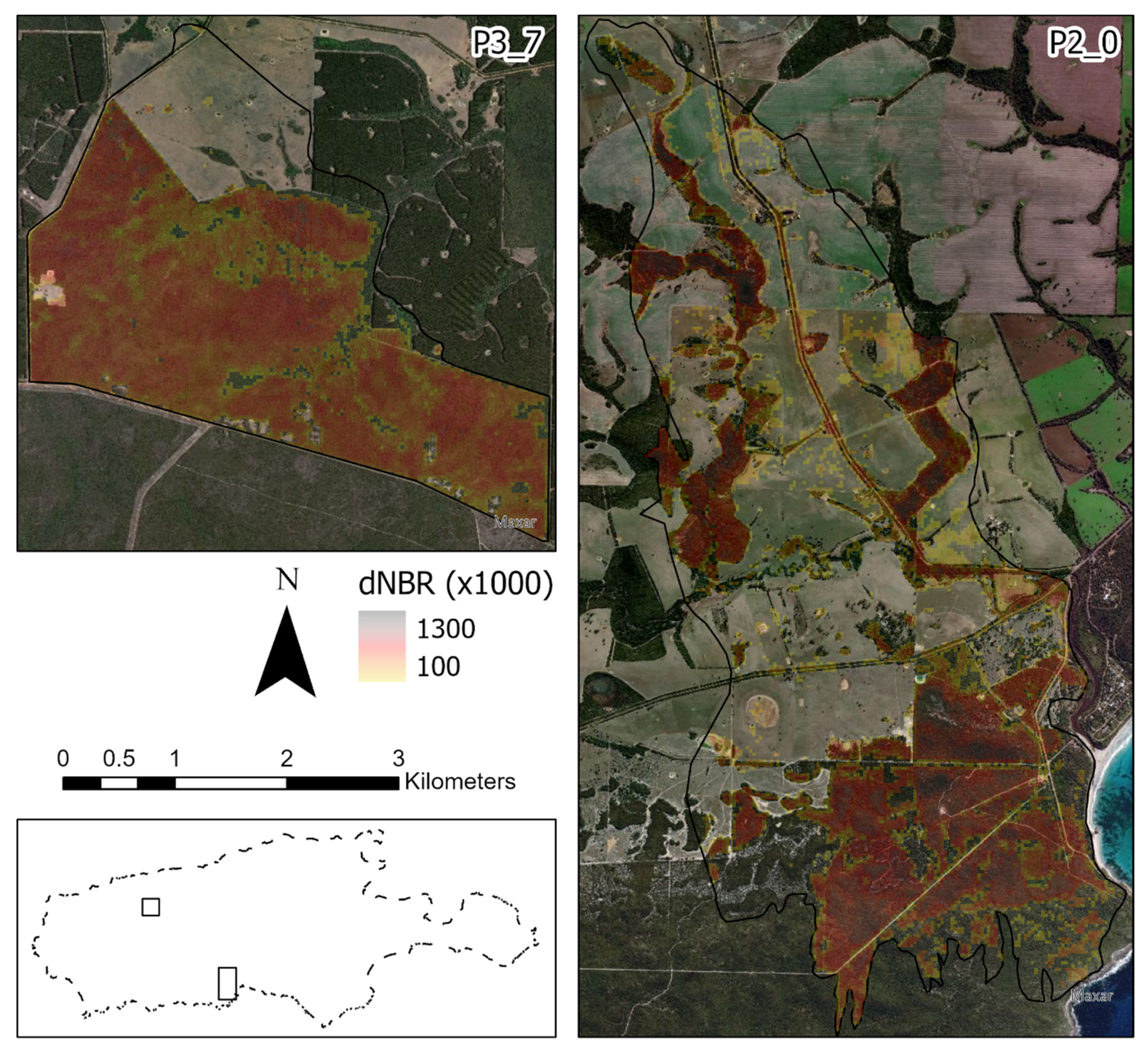
3.2. Severity: Landscape-Level Influences
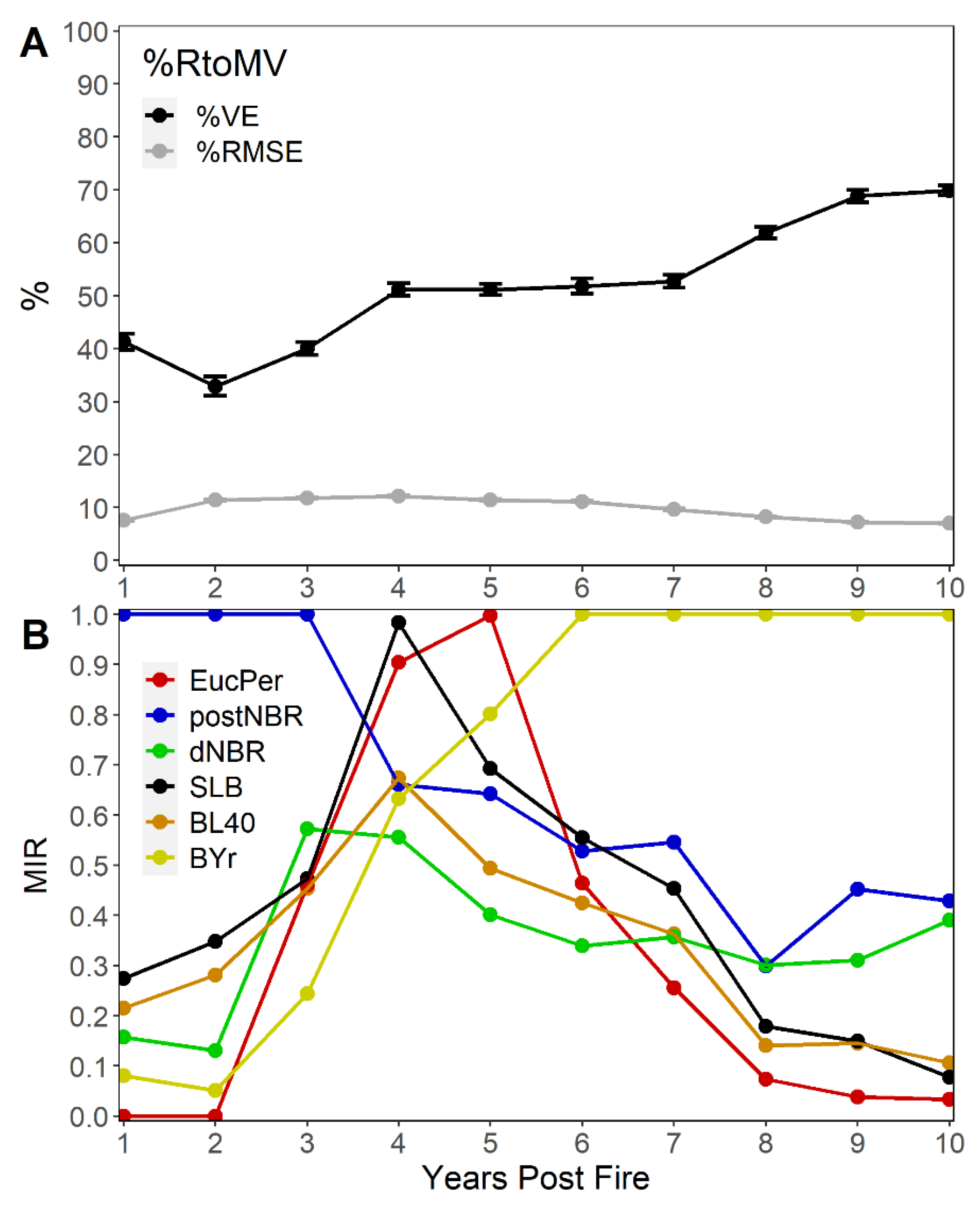
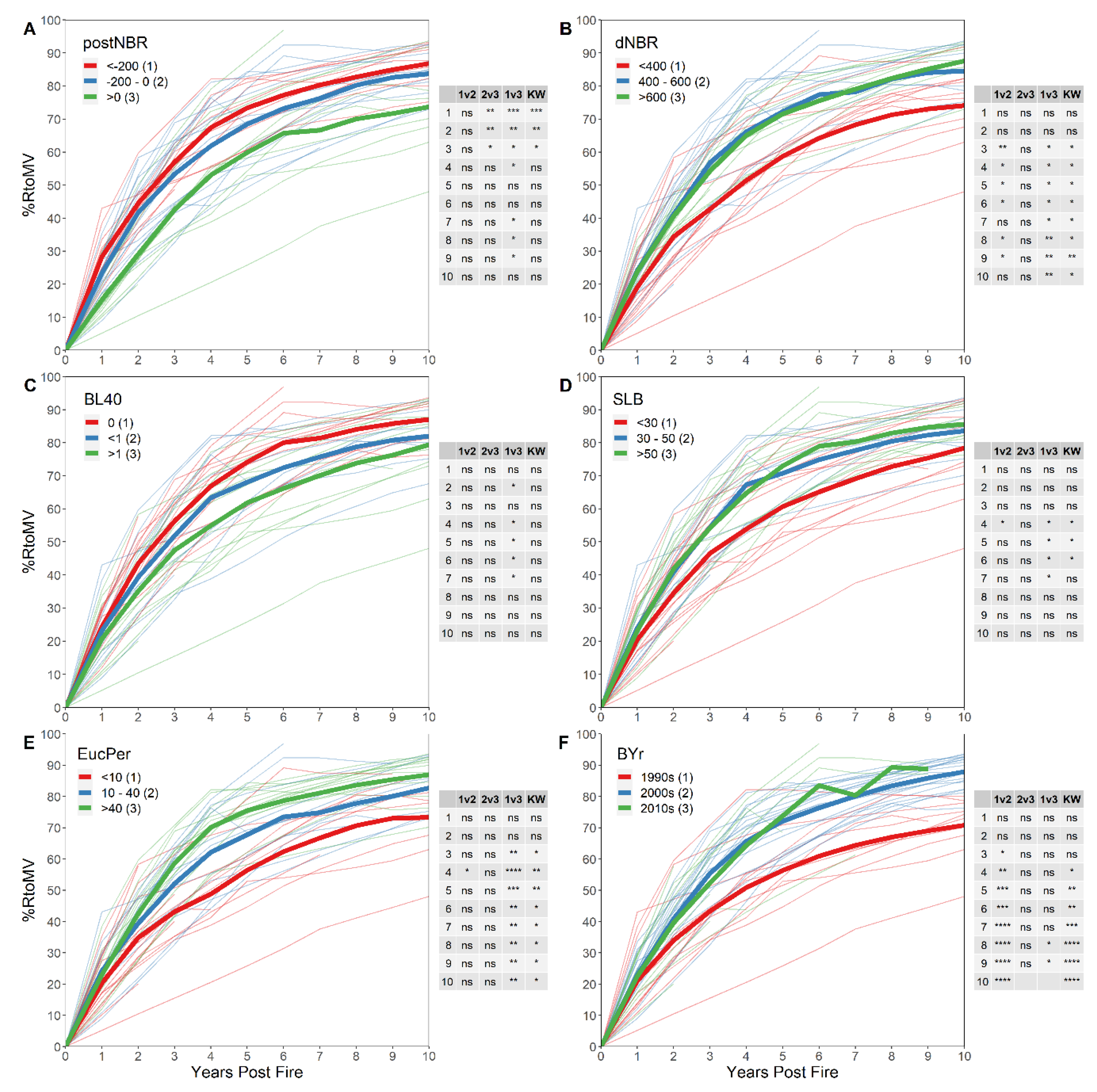
3.3. Recovery: Landscape-Level Influences
4. Discussion
4.1. Fire History in the Context of the 2019–2020 Bushfires
4.2. Influences on Burn Severity
4.3. Influences on Post-Fire Recovery
4.4. Limitations
5. Conclusions
Author Contributions
Funding
Acknowledgments
Conflicts of Interest
Appendix A


References
- Richards, L.; Brew, N.; Smith, L. 2019–20 Australian Bushfires—Frequently Asked Questions: A Quick Guide. Available online: https://www.aph.gov.au/About_Parliament/Parliamentary_Departments/ Parliamentary_Library/pubs/rp/rp1920/Quick_Guides/AustralianBushfires (accessed on 1 August 2020).
- Royal Commission into National Natural Disaster Arrangements. Interim Observations, 31 August 2020. Available online: https://naturaldisaster.royalcommission.gov.au/publications/interim-observations-1 (accessed on 15 November 2020).
- Khalil, S. Australia Fires: ‘Apocalypse’ Comes to Kangaroo Island. Available online: https://www.bbc.com/news/world-australia-51102658 (accessed on 3 August 2020).
- Tarabay, J. There’s No Place Like Kangaroo Island. Can It Survive Australia’s Fires? Available online: https://www.nytimes.com/2020/02/04/world/australia/kangaroo-island-fire.html (accessed on 24 June 2020).
- Clarke, H.G.; Smith, P.L.; Pitman, A.J. Regional signatures of future fire weather over eastern Australia from global climate models. Int. J. Wildland Fire 2011, 20, 550–562. [Google Scholar] [CrossRef]
- Australian Government: Bureau of Meteorology. Historical Weather Observations and Statistics. Available online: http://www.bom.gov.au/climate/data-services/station-data.shtml (accessed on 15 May 2020).
- Attiwill, P.M.; Adams, M.A. Mega-fires, inquiries and politics in the eucalypt forests of Victoria, South-Eastern Australia. For. Ecol. Manag. 2013, 294, 45–53. [Google Scholar] [CrossRef]
- Yang, J.; Tian, H.; Tao, B.; Ren, W.; Lu, C.; Pan, S.; Liu, Y. Century-scale patterns and trends of global pyrogenic carbon emissions and fire influences on terrestrial carbon balance. Glob. Biogeochem. Cycles 2015, 29, 1549–1566. [Google Scholar] [CrossRef]
- Viedma, O.; Meliá, J.; Segarra, D.; García-Haro, J. Modeling rates of ecosystem recovery after fires by using Landsat TM data. Remote Sens. Environ. 1997, 61, 383–398. [Google Scholar] [CrossRef]
- White, J.D.; Ryan, K.C.; Key, C.C.; Running, S.W. Remote sensing for forest fire severity and vegetation recovery. Int. J. Wildland Fire 1996, 6, 125–136. [Google Scholar] [CrossRef] [Green Version]
- Wulder, M.A.; Masek, J.G.; Cohen, W.B.; Loveland, T.R.; Woodcock, C.E. Opening the archive: How free data has enabled the science and monitoring promise of Landsat. Remote Sens. Environ. 2012, 122, 2–10. [Google Scholar] [CrossRef]
- Vicente-Serrano, S.M.; Pérez-Cabello, F.; Lasanta, T. Pinus halepensis regeneration after a wildfire in a semiarid environment: Assessment using multitemporal Landsat images. Int. J. Wildland Fire 2011, 20, 195–208. [Google Scholar] [CrossRef]
- Gorelick, N.; Hancher, M.; Dixon, M.; Ilyushchenko, S.; Thau, D.; Moore, R. Google earth engine: Planetary-scale geospatial analysis for everyone. Remote Sens. Environ. 2017, 202, 18–27. [Google Scholar] [CrossRef]
- Kennedy, R.E.; Yang, Z.; Gorelick, N.; Braaten, J.; Cavalcante, L.; Cohen, W.B.; Healey, S. Implementation of the LandTrendr algorithm on google earth engine. Remote Sens. 2018, 10, 691. [Google Scholar] [CrossRef] [Green Version]
- Kennedy, R.E.; Yang, Z.; Cohen, W.B. Detecting trends in forest disturbance and recovery using yearly Landsat time series: 1. LandTrendr—Temporal segmentation algorithms. Remote Sens. Environ. 2010, 114, 2897–2910. [Google Scholar] [CrossRef]
- Bright, B.C.; Hudak, A.T.; Kennedy, R.E.; Braaten, J.D.; Khalyani, A.H. Examining post-fire vegetation recovery with Landsat time series analysis in three Western North American forest types. Fire Ecol. 2019, 15. [Google Scholar] [CrossRef] [Green Version]
- Quintero, N.; Viedma, O.; Urbieta, I.R.; Moreno, J.M. Assessing landscape fire hazard by multitemporal automatic classification of Landsat time series using the google earth engine in West-Central Spain. Forests 2019, 10, 518. [Google Scholar] [CrossRef] [Green Version]
- Frazier, R.J.; Coops, N.C.; Wulder, M.A.; Hermosilla, T.; White, J.C. Analyzing spatial and temporal variability in short-term rates of post-fire vegetation return from Landsat time-series. Remote Sens. Environ. 2018, 205, 32–45. [Google Scholar] [CrossRef]
- Meng, R.; Dennison, P.E.; Huang, C.; Moritz, M.A.; D’Antonio, C. Effects of fire severity and post-fire climate on short-term vegetation recovery of mixed-conifer and red fir forests in the Sierra Nevada mountains of California. Remote Sens. Environ. 2015, 171, 311–325. [Google Scholar] [CrossRef]
- Pickell, P.D.; Hermosilla, T.; Frazier, R.J.; Coops, N.C.; Wulder, M.A. Forest recovery trends derived from Landsat time series for North American boreal forests. Int. J. Remote Sens. 2015, 37, 138–149. [Google Scholar] [CrossRef]
- White, J.C.; Wulder, M.A.; Hermosilla, T.; Coops, N.C.; Hobart, G.W. A Nationwide annual characterization of 25 years of forest disturbance and recovery for Canada using Landsat time series. Remote Sens. Environ. 2017, 194, 303–321. [Google Scholar] [CrossRef]
- Sever, L.; Leach, J.; Bren, L. Remote sensing of post-fire vegetation recovery; a study using Landsat 5 TM imagery and NDVI in North-East Victoria. J. Spat. Sci. 2012, 57, 175–191. [Google Scholar] [CrossRef]
- Epting, J.; Verbyla, D. Landscape-level interactions of prefire vegetation, burn severity, and postfire vegetation over a 16-year period in interior Alaska. Can. J. For. Res. 2005, 35, 1367–1377. [Google Scholar] [CrossRef] [Green Version]
- Liu, Z. Effects of climate and fire on short-term vegetation recovery in the boreal larch forests of Northeastern China. Sci. Rep. 2016, 6, 37572. [Google Scholar] [CrossRef] [Green Version]
- Schroeder, T.A.; Wulder, M.A.; Healey, S.P.; Moisen, G.G. Mapping wildfire and clearcut harvest disturbances in boreal forests with Landsat time series data. Remote Sens. Environ. 2011, 6, 1421–1433. [Google Scholar] [CrossRef]
- Hislop, S.; Jones, S.; Soto-Berelov, M.; Skidmore, A.; Haywood, A.; Nguyen, T.H. Using Landsat spectral indices in time-series to assess wildfire disturbance and recovery. Remote Sens. 2018, 10, 460. [Google Scholar] [CrossRef] [Green Version]
- Fernandez-Manso, A.; Quintano, C.; Roberts, D.A. Burn severity influence on post-fire vegetation cover resilience from Landsat MESMA fraction images time series in Mediterranean forest ecosystems. Remote Sens. Environ. 2016, 184, 112–123. [Google Scholar] [CrossRef]
- Yang, J.; Pan, S.; Dangal, S.; Zhang, B.; Wang, S.; Tian, H. Continental-scale quantification of post-fire vegetation greenness recovery in temperate and boreal North America. Remote Sens. Environ. 2017, 199, 277–290. [Google Scholar] [CrossRef]
- Malak, D.A.; Pausas, J.G. Fire regime and post-fire normalized difference vegetation index changes in the Eastern Iberian peninsula (Mediterranean basin). Int. J. Wildland Fire 2006, 15, 407–413. [Google Scholar] [CrossRef]
- Díaz-Delgado, R.; Lloret, F.; Pons, X. Influence of fire severity on plant regeneration by means of remote sensing imagery. Int. J. Remote Sens. 2003, 24, 1751–1763. [Google Scholar] [CrossRef]
- Meng, R.; Dennison, P.E.; D’Antonio, C.M.; Moritz, M.A. Remote sensing analysis of vegetation recovery following short-interval fires in Southern California shrublands. PLoS ONE 2014, 9, 110637. [Google Scholar] [CrossRef] [Green Version]
- Hammill, K.A.; Bradstock, R.A. Remote sensing of fire severity in the Blue Mountains: Influence of vegetation type and inferring fire intensity. Int. J. Wildland Fire 2006, 15, 213–226. [Google Scholar] [CrossRef]
- Lippitt, C.L.; Stow, D.A.; O’Leary, J.F.; Franklin, J. Influence of short-interval fire occurrence on post-fire recovery of fire-prone shrublands in California, USA. Int. J. Wildland Fire 2013, 22, 184–193. [Google Scholar] [CrossRef]
- Boer, M.M.; Sadler, R.J.; Wittkuhn, R.S.; McCaw, L.; Greirson, P.F. Long-term impacts of prescribed burning on regional extent and incidence of wildfires—Evidence from 50 years of active fire management in SW Australian forests. Forest Ecol. Manag. 2009, 259, 132–142. [Google Scholar] [CrossRef]
- Dowie, D. Age Class Distributions of Seven Vegetation Groups on Kangaroo Island. Fahrenheit 451—A Fire Management Program for Biodiversity and Asset Protection on Kangaroo Island; Government of South Australia: Adelaide, Australia, 2006.
- Estes, B.L.; Knapp, E.E.; Skinner, C.N.; Miller, J.D.; Preisler, H.K. Factors influencing fire severity under moderate burning conditions in the Klamath Mountains, northern California, USA. Ecosphere 2017, 8. [Google Scholar] [CrossRef] [Green Version]
- Garcia-Llamas, P.; Suárez-Seoane, S.; Taboada, A.; Fernández-García, V.; Fernández-Guisuraga, J.M.; Fernández-Manso, A.; Quintano, C.; Marcos, E.; Calvo, L. Assessment of the influence of biophysical properties related to fuel conditions on fire severity using remote sensing techniques: A Case study on a large fire in NW Spain. Int. J. Wildland Fire 2019, 28, 512–520. [Google Scholar] [CrossRef]
- Parks, S.A.; Miller, C.; Nelson, C.R.; Holden, Z.A. Previous fires moderate burn severity of subsequent wildland fires in two large western US wilderness areas. Ecosystems 2013, 17, 29–42. [Google Scholar] [CrossRef] [Green Version]
- Stevens-Rumann, C.S.; Prichard, S.J.; Strang, E.K.; Morgan, P. Prior wildfires influence burn severity of subsequent large fires. Can. J. For. Res. 2016, 46, 1375–1385. [Google Scholar] [CrossRef] [Green Version]
- Kangaroo Island Council. Kangaroo Island Development Plan. Available online: https://www.kangarooisland.sa.gov.au/council/plans/development/plan (accessed on 3 August 2020).
- Paton, D.C.; Prescott, A.M.; Davies, R.J.P.; Heard, L.M. The distribution, status and threats to temperate woodlands in South Australia. In Temperate Eucalypt Woodlands in Australia: Biology, Conservation and Restoration; Hobbs, R.J., Yates, C.J., Eds.; Surrey Beatty & Sons: Chipping Norton, Australia, 2000; pp. 57–85. [Google Scholar]
- Department of Agriculture, Water and the Environment. National Vegetation Information System (NVIS). Available online: https://www.environment.gov.au/land/native-vegetation/national-vegetation-information-system (accessed on 16 November 2020).
- Australian Government: Department of Agriculture, Water and the Environment. Australian Land Use and Management Classification Version 8 (October 2016). Available online: https://www.agriculture.gov.au/abares/aclump/land-use/alum-classification (accessed on 3 February 2020).
- Government of South Australia: Department for Environment and Water. Conservation Reserve Boundaries. Available online: https://data.sa.gov.au/data/dataset/conservation-reserve-boundaries (accessed on 13 November 2020).
- Government of South Australia: Department for Environment and Water. Bushfires and Prescribed Burns History. Available online: https://data.sa.gov.au/data/dataset/e5434c77-9815-48e6-8ea7-fb35c78f6786 (accessed on 3 April 2020).
- Peace, M.; Mills, G. A Case Study of the 2007 Kangaroo Island Bushfires; Technical Report No. 053; Australian Government: Bureau of Meteorology, The Centre for Australian Weather and Climate Research: Melbourne, Australia, 2012.
- Zhu, Z.; Wang, S.; Woodcock, C.E. Improvement and Expansion of the FMASK algorithm: Cloud, cloud shadow, and snow detection for Landsats 4–7, 8, and sentinel 2 images. Remote Sens. Environ. 2015, 159, 269–277. [Google Scholar] [CrossRef]
- Masek, J.G.; Vermote, E.F.; Saleous, N.E.; Wolfe, R.; Hall, F.G.; Huemmrich, K.F.; Gao, F.; Kutler, J.; Lim, T.K. A Landsat surface reflectance dataset for North America, 1990–2000. IEEE Geosci. Remote Sens. Lett. 2006, 3, 68–72. [Google Scholar] [CrossRef]
- Vermote, E.; Justice, C.; Claverie, M.; Franch, B. Preliminary analysis of the performance of the Landsat 8/OLI land surface reflectance product. Remote Sens. Environ. 2016, 185, 46–56. [Google Scholar] [CrossRef]
- Roy, D.P.; Kovalskyy, V.; Zhang, H.K.; Vermote, E.F.; Yan, L.; Kumar, S.S.; Egorov, A. Characterization of Landsat-7 to Landsat-8 reflective wavelength and normalized difference vegetation index continuity. Remote Sens. Environ. 2016, 185, 57–70. [Google Scholar] [CrossRef] [Green Version]
- Flood, N. Seasonal composite Landsat TM/ETM+ images using the medoid (a multi-dimensional median). Remote Sens. 2013, 5, 6481–6500. [Google Scholar] [CrossRef] [Green Version]
- Lehmann, E.A.; Wallace, J.F.; Caccetta, P.A.; Furby, S.L.; Zdunic, K. Forest cover trends from time series Landsat data for the Australian continent. Int. J. Appl. Earth Obs. Geoinf. 2013, 21, 453–462. [Google Scholar] [CrossRef]
- Key, C.H.; Benson, N.C. Landscape assessment: Remote sensing of severity, the normalized burn ratio. In FIREMON: Fire Effects Monitoring and Inventory System; USDA Forest Service, Rocky Mountain Research Station, Fort Collins: Denver, CO, USA, 2006; pp. 305–325. [Google Scholar]
- Yang, Y.; Erskine, P.D.; Lechner, A.M.; Mulligan, D.; Zhang, S.; Wang, Z. Detecting the dynamics of vegetation disturbance and recovery in surface mining area via Landsat imagery and LandTrendr algorithm. J. Clean. Prod. 2018, 178, 353–362. [Google Scholar] [CrossRef]
- NASA Jet Propulsion Laboratory. U.S. Releases Enhanced Shuttle Land Elevation Data. Available online: https://www.jpl.nasa.gov/news/news.php?release=2014-321 (accessed on 21 March 2020).
- Weiss, A.D. Topographic position and landforms analysis. In Proceedings of the Presented at ESRI Users Conference, San Diego, CA, USA, 9–13 July 2001. [Google Scholar]
- Beven, K.J.; Kirkby, M.J. A physically based, variable contributing area model of basin hydrology. Hydrol. Sci. Bull. 1979, 24, 43–69. [Google Scholar] [CrossRef] [Green Version]
- Breiman, L. Random Forests. Mach. Learn. 2001, 45, 5–32. [Google Scholar] [CrossRef] [Green Version]
- Liaw, A.; Wiener, M. Classification and regression by random forest. R News 2002, 2, 18–22. [Google Scholar]
- Murphy, M.A.; Evans, J.S.; Storfer, A.S. Quantify bufo boreas connectivity in Yellowstone national park with landscape genetics. Ecology 2010, 91, 252–261. [Google Scholar] [CrossRef] [PubMed] [Green Version]
- Tolhurst, K.G.; McCarthy, G. Effect of prescribed burning on wildfire severity: A landscape-scale case study from the 2003 fires in Victoria. Aust. For. 2016, 79. [Google Scholar] [CrossRef]
- Government of South Australia: Kangaroo Island Landscape Board. Bushfire Recovery. Available online: https://landscape.sa.gov.au/ki/land-and-water/Bushfire_recovery (accessed on 3 August 2020).
- Bennett, L.T.; Bruce, M.J.; MacHunter, J.; Kohout, M.; Tanase, M.A.; Aponte, C. Mortality and recruitment of fire-tolerant eucalypts as influenced by wildfire severity and recent prescribed fire. For. Ecol. Manag. 2016, 380, 107–117. [Google Scholar] [CrossRef]
- Haslem, A.; Kelly, L.T.; Nimmo, D.G.; Watson, S.J.; Kenny, S.A.; Taylor, R.S.; Bennett, A.F. Habitat or fuel? Implications of long-term, post-fire dynamics for the development of key resources for fauna and fire. J. Appl. Ecol. 2010, 48, 247–256. [Google Scholar] [CrossRef]
- Butt, N.; Pollock, L.J.; McAlpine, C.A. Eucalypts face increasing climate stress. Ecol. Evol. 2013, 3, 5011–5022. [Google Scholar] [CrossRef]
- Government of South Australia: Department of Environment and Water. Find out how South Australia’s Flinders Chase National Park is recovering post-bushfire. Available online: https://www.environment.sa.gov.au/goodliving/posts/2020/04/flinders-chase-plants-regenerating (accessed on 24 June 2020).
- Ye, S.; Rogan, J.; Zhu, Z.; Eastman, J.R. A near-real-time approach for monitoring forest disturbance using Landsat time series: Stochastic continuous change detection. Remote Sens. Environ. 2020, 252, 112167. [Google Scholar] [CrossRef]


| Parameters | Default | Selected |
|---|---|---|
| maxSegments | 6 | 8 |
| spikeThreshold | 0.9 | 0.9 |
| vertexCountOvershoot | 3 | 3 |
| preventOneYearRecovery | TRUE | TRUE |
| recoveryThreshold | 0.25 | 0.75 |
| pvalThreshold | 0.05 | 0.05 |
| bestModelProportion | 0.75 | 0.75 |
| minObservationsNeeded | 6 | 6 |
| Accuracy | ||
| All | 70% | 81% |
| Forest | 80% | 93% |
| ID | Fire Season | Date | Extent (Burned) km2 | Elevation (m) | Vegetation Species |
|---|---|---|---|---|---|
| P1_5 | 1988–1989 | 20-October | 2.4 (1.2) | 195.4 ± 15.7 | Eucalyptus diversifolia |
| P1_0 | 1989–1990 | 22-November | 6.7 (1.9) | 37.7 ± 9.6 | E. diversifolia |
| P1_1 | 1989–1990 | 22-March | 1.4 (0.9) | 71.9 ± 6.9 | E. diversifolia |
| P1_4 | 1990–1991 | 31-December | 132.6 (90.9) | 221.0 ± 55.9 | E. remota |
| P1_2 | 1990–1991 | 09-February | 1.6 (0.7) | 16.0 ± 4.6 | E. remota |
| P1_3 | 1991–1992 | 31-December | 248.7 (194.6) | 136.2 ± 67.1 | E. baxteri |
| P2_1 | 1993–1994 | 09-December | 1.5 (0.4) | 63.7 ± 5.2 | E. diversifolia |
| P2_2 | 1993–1994 | 24-March | 2.3 (1.9) | 93.4 ± 26.9 | E. diversifolia |
| P2_0 | 1994–1995 | 11-December | 22.0 (9.8) | 32.9 ± 17.3 | Leucopogon parviflorus |
| P2_3 | 1996–1997 | 15-December | 242.7 (194.3) | 36.7 ± 15.7 | E. diversifolia |
| P2_4 | 1996–1997 | 27-March | 44.2 (23.3) | 152.2 ± 43.9 | E. remota |
| P3_4 | 2000–2001 | 31-January | 21.5 (19.7) | 195.7 ± 34.9 | E. diversifolia |
| P3_7 | 2000–2001 | 18-February | 10.7 (8.1) | 286.5 ± 11.1 | E. baxteri |
| P3_6 | 2002–2003 | 02-November | 63.7 (62.7) | 208.4 ± 61.0 | E. diversifolia |
| P3_9 | 2003–2004 | 14-January | 2.5 (1.2) | 26.2 ± 3.7 | E. cladocalyx |
| P3_5 | 2004–2005 | 19-December | 1.3 (0.9) | 15.2 ± 6.4 | E. remota |
| P3_2 | 2004–2005 | 28-April | 17.6 (5.5) | 81.7 ± 22.9 | Undifferentiated |
| P3_3 | 2004–2005 | 28-April | 1.6 (0.2) | 137.5 ± 35.4 | E. remota |
| P3_10 | 2005–2006 | 20-January | 31.6 (31.5) | 80.7 ± 10.4 | E. baxteri |
| P3_1 | 2005–2006 | 21-January | 1.1 (0.9) | 268.8 ± 2.3 | E. remota |
| P3_0 | 2006–2007 | 11-October | 2.3 (2.0) | 43.4 ± 7.2 | E. diversifolia |
| P3_11 | 2006–2007 | 11-October | 6.3 (5.4) | 94.5 ± 10.3 | E. diversifolia |
| P3_12 | 2006–2007 | 11-October | 5.5 (4.4) | 123.6 ± 32.2 | E. baxteri |
| P3_8 | 2006–2007 | 11-November | 23.6 (21.8) | 258.0 ± 24 | E. cladocalyx |
| P4_2 | 2007–2008 | 07-September | 8.7 (8.4) | 92.6 ± 32.5 | E. cladocalyx |
| P4_0 | 2007–2008 | 06-December | 2.3 (1.6) | 237.8 ± 10.5 | E. cladocalyx |
| P4_1 | 2007–2008 | 06-December | 29.5 (24.5) | 161.4 ± 44.5 | E. diversifolia |
| P4_3 | 2007–2008 | 06-December | 162.9 (161.0) | 32.9 ± 11.0 | E. diversifolia |
| P4_4 | 2007–2008 | 06-December | 50.3 (18.9) | 76.8 ± 36.8 | E. baxteri |
| P4_5 | 2007–2008 | 06-December | 604.7 (599.8) | 154.2 ± 67.1 | E. remota |
| P5_0 | 2010–2011 | 04-December | 1.6 (0.2) | 19.4 ± 7.2 | E. diversifolia |
| P5_10 | 2010–2011 | 08-February | 3.2 (3.0) | 179.6 ± 14.4 | Undifferentiated |
| P5_2 | 2011–2012 | 14-March | 4.3 (3.7) | 37.7 ± 12.7 | E. diversifolia |
| P5_3 | 2011–2012 | 06-April | 2.5 (2.0) | 205.1 ± 36.5 | E. remota |
| P5_5 | 2013–2014 | 22-April | 4.5 (3.2) | 34.7 ± 6.5 | E. diversifolia |
| P5_6 | 2014–2015 | 31-May | 3.7 (3.4) | 240.3 ± 25.5 | E. diversifolia |
| P5_8 | 2015–2016 | 25-October | 1.5 (1.5) | 277.6 ± 12.7 | E. remota |
| P5_4 | 2015–2016 | 20-March | 1.8 (1.1) | 28.6 ± 3.2 | Unclassifiable |
| P5_9 | 2016–2017 | 18-April | 3.0 (2.6) | 275.0 ± 18.0 | E. remota |
| P5_12 | 2016–2017 | 18-April | 2.0 (1.9) | 263.9 ± 5.6 | E. remota |
| P5_7 | 2017–2018 | 24-January | 1.1 (0.3) | 47.2 ± 7.3 | E. cosmophylla |
| P5_1 | 2017–2018 | 08-February | 3.7 (2.6) | 84.0 ± 55.2 | Undifferentiated |
| P5_11 | 2018–2019 | 06-December | 11.3 (8.9) | 103.0 ± 24.5 | E. baxteri |
| P6_0 | 2019–2020 | 20-December | 8.4 (2.9) | 76.7 ± 18.2 | E. cladocalyx |
| P6_1 | 2019–2020 | 21-December | 165.5 (132.3) | 183.1 ± 56.8 | E. cladocalyx |
| P6_2 | 2019–2020 | 21-December | 2.1 (1.6) | 65.2 ± 7.1 | E. diversifolia |
| P6_3 | 2019–2020 | 30-December | 1918.8 (1630.8) | 152.6 ± 72.7 | E. remota |
| Variable | Level | Category | Description |
|---|---|---|---|
| Burned extent (BExt) | Landscape | Current burn | Area (km2) burned in fire polygon, log10 transformed |
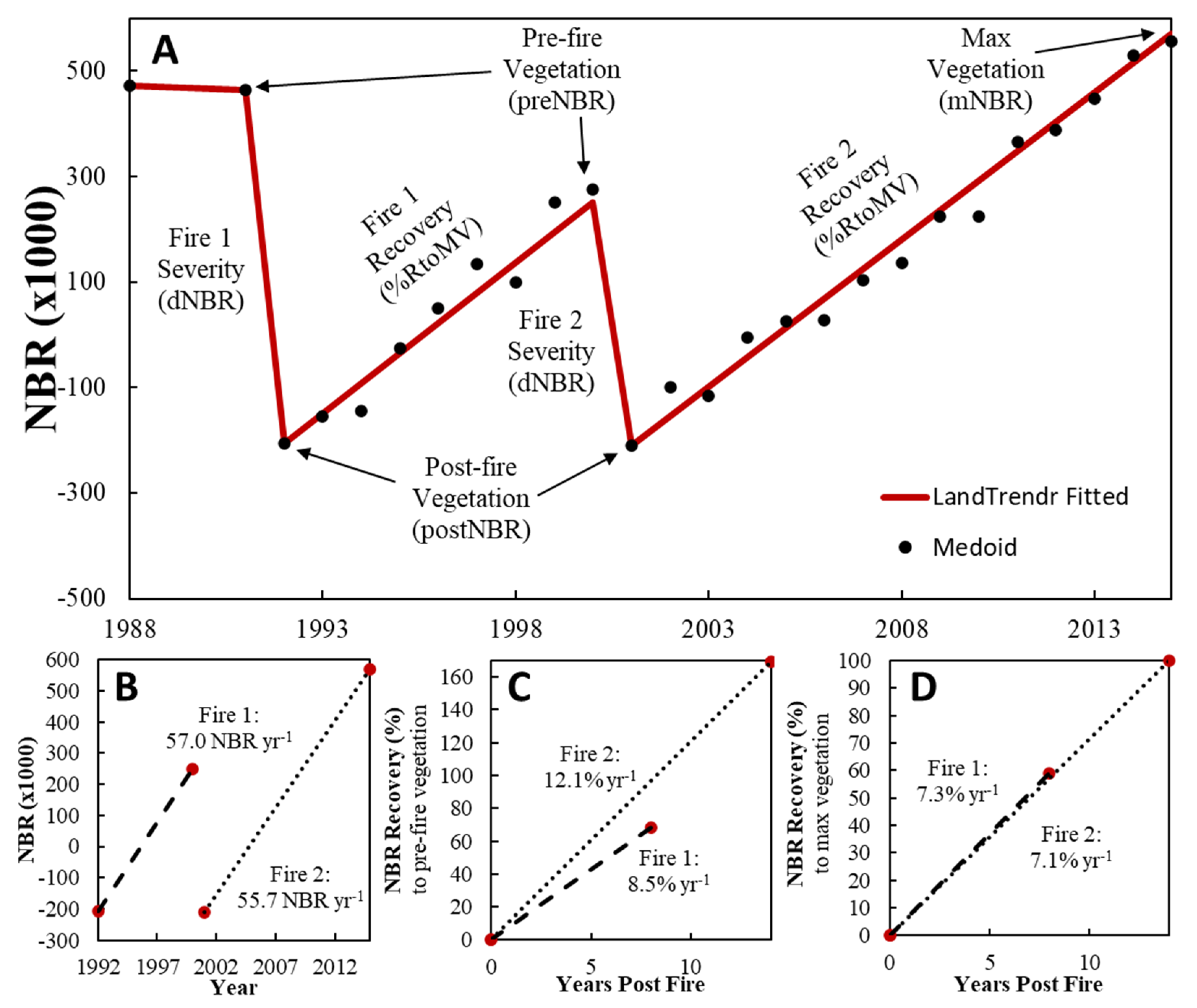
| Pre-fire vegetation (preNBR) | Pixel | Vegetation structure | NBR value the last year before burn x1000 (Figure 4) |
| Max vegetation (mNBR) | Pixel | Vegetation structure | Max NBR value across full time-series x1000 (Figure 4) |
| Land use percentage | Pixel | Vegetation structure | Land use class for each pixel, used to build fire-level composition |
| Vegetation group percentage | Pixel | Vegetation structure | Vegetation group for each pixel, used to build fire-level compsition |
| Most common land use | Landscape | Vegetation structure | Highest percentage land use across pixels |
| Most common vegetation group | Landscape | Vegetation structure | Highest percentage vegetation group across pixels |
| Most common species | Landscape | Vegetation structure | Highest percentage dominant species across pixels |
| Years since last burn (SLB) | Pixel | Fire history | Number of years since the last burn, pixels with no recorded burns given a value of 70 (i.e., at least 70 years since the last burn) |
| Times burned in last X years (BLX) | Pixel | Fire history | Number of times burned in the last X (70, 60, 50, 40, 30, 20, 10) years |
| Elevation (ELV) | Pixel | Topography | Elevation above sea level (m) |
| Slope (SLP) | Pixel | Topography | Slope (°) calculated from ELV |
| Aspect | Pixel | Topography | Aspect (°) calculated from ELV |
| Topographic position index (TPIX) | Pixel | Topography | Difference (m) between the center pixel and average ELV of an X by X (3, 5, 9, 15, 31, 65, 111) pixel moving window [56] |
| Topographic wetness index | Pixel | Topography | Ln((Flow Accumulation + 1)/Tan (((SLP) × π)/180))) [57] |
| Fire season (BYr) | Landscape | Current burn | Year corresponding with the end of fire season when burn occurred |
| Time of year | Landscape | Current burn | Number of days from December 31st when burn occurred |
| Missing data (MD) | Landscape | Indicates if a burn occurred when and where no cloud-free Landsat data were available (i.e., one of dNBR years impacted by missing data) | |
| Post-fire vegetation (postNBR) | Pixel | Current burn | NBR value the first year after burn x1000, only tested in %RtoMV models (Figure 4) |
| Burn severity (dNBR) | Pixel | Current burn | NBR difference between preNBR and postNBR x1000, only tested in %RtoMV models (Figure 4) |
Publisher’s Note: MDPI stays neutral with regard to jurisdictional claims in published maps and institutional affiliations. |
© 2020 by the authors. Licensee MDPI, Basel, Switzerland. This article is an open access article distributed under the terms and conditions of the Creative Commons Attribution (CC BY) license (http://creativecommons.org/licenses/by/4.0/).
Share and Cite
Bonney, M.T.; He, Y.; Myint, S.W. Contextualizing the 2019–2020 Kangaroo Island Bushfires: Quantifying Landscape-Level Influences on Past Severity and Recovery with Landsat and Google Earth Engine. Remote Sens. 2020, 12, 3942. https://0-doi-org.brum.beds.ac.uk/10.3390/rs12233942
Bonney MT, He Y, Myint SW. Contextualizing the 2019–2020 Kangaroo Island Bushfires: Quantifying Landscape-Level Influences on Past Severity and Recovery with Landsat and Google Earth Engine. Remote Sensing. 2020; 12(23):3942. https://0-doi-org.brum.beds.ac.uk/10.3390/rs12233942
Chicago/Turabian StyleBonney, Mitchell T., Yuhong He, and Soe W. Myint. 2020. "Contextualizing the 2019–2020 Kangaroo Island Bushfires: Quantifying Landscape-Level Influences on Past Severity and Recovery with Landsat and Google Earth Engine" Remote Sensing 12, no. 23: 3942. https://0-doi-org.brum.beds.ac.uk/10.3390/rs12233942