Article

Water Quality Retrieval from PRISMA Hyperspectral Images: First Experience in a Turbid Lake and Comparison with Sentinel-2

by
Milad Niroumand-Jadidi
1,*,
Francesca Bovolo
1 and
Lorenzo Bruzzone
2
1
Center for Information and Communication Technology, Fondazione Bruno Kessler, Via Sommarive, 18 I-38123 Trento, Italy
2
Department of Information Engineering and Computer Science, University of Trento, Via Sommarive, 5 I-38123 Trento, Italy
*
Author to whom correspondence should be addressed.
Remote Sens. 2020, 12(23), 3984; https://0-doi-org.brum.beds.ac.uk/10.3390/rs12233984
Submission received: 4 November 2020 / Revised: 1 December 2020 / Accepted: 4 December 2020 / Published: 6 December 2020
(This article belongs to the Special Issue Remote Sensing of Lake Properties and Dynamics)

Abstract

:
A new era of spaceborne hyperspectral imaging has just begun with the recent availability of data from PRISMA (PRecursore IperSpettrale della Missione Applicativa) launched by the Italian space agency (ASI). There has been pre-launch optimism that the wealth of spectral information offered by PRISMA can contribute to a variety of aquatic science and management applications. Here, we examine the potential of PRISMA level 2D images in retrieving standard water quality parameters, including total suspended matter (TSM), chlorophyll-a (Chl-a), and colored dissolved organic matter (CDOM) in a turbid lake (Lake Trasimeno, Italy). We perform consistency analyses among the aquatic products (remote sensing reflectance (Rrs) and constituents) derived from PRISMA and those from Sentinel-2. The consistency analyses are expanded to synthesized Sentinel-2 data as well. By spectral downsampling of the PRISMA images, we better isolate the impact of spectral resolution in retrieving the constituents. The retrieval of constituents from both PRISMA and Sentinel-2 images is built upon inverting the radiative transfer model implemented in the Water Color Simulator (WASI) processor. The inversion involves a parameter (gdd) to compensate for atmospheric and sun-glint artifacts. A strong agreement is indicated for the cross-sensor comparison of Rrs products at different wavelengths (average R ≈ 0.87). However, the Rrs of PRISMA at shorter wavelengths (<500 nm) is slightly overestimated with respect to Sentinel-2. This is in line with the estimates of gdd through the inversion that suggests an underestimated atmospheric path radiance of PRISMA level 2D products compared to the atmospherically corrected Sentinel-2 data. The results indicate the high potential of PRISMA level 2D imagery in mapping water quality parameters in Lake Trasimeno. The PRISMA-based retrievals agree well with those of Sentinel-2, particularly for TSM.

Graphical Abstract

1. Introduction

The applications of Earth observation data are becoming more and more widespread in the monitoring and management of aquatic systems [1,2]. This is due to the underpinning role of remote sensing in providing spatially and temporally distributed data, whereas traditional field measurements fall short in capturing the spatiotemporal dynamics of the inland/coastal biophysical properties [3,4,5]. Having accurate and timely information on biophysical parameters such as water quality and habitat indicators is crucial for sustainable management of a variety of aquatic ecosystem services, such as urban and agricultural water supply, fisheries, tourism, and recreation activities [4,5]. Furthermore, this kind of information contributes to a better understanding of processes such as eutrophication and harmful algal blooms, carbon cycle, as well as climate change impacts [6,7,8]. Among water quality parameters, the concentration of chlorophyll-a (Chl-a), which is in turn an indicator of the phytoplankton abundance, can be considered a key parameter for assessment of the primary production, the trophic status, and the quality of water [9]. Harmful algal blooms (HABs) can endanger aquatic and human health. The monitoring of HABs requires timely and spatially distributed information about Chl-a concentration [10,11]. Total suspended matter (TSM) is a measure of organic and mineral solids suspended in the water column [12]. A high concentration of TSM can significantly reduce the light availability for primary production and thus lead to degradation of aquatic habitat, and limit fisheries and drinking water resources [13]. Colored dissolved organic matter (CDOM) is another key water quality indicator that is closely linked to the carbon content. Spatiotemporal monitoring of CDOM can contribute to studies of carbon cycle, aquatic ecology, climate change, and water treatment projects [14,15,16].
Remotely sensed data have long been leveraged in quantification and mapping of optically active constituents such as Chl-a, TSM, and CDOM. Information on bathymetry and benthic habitats such as submerged aquatic vegetation can be also derived from water-leaving spectral data [17,18,19]. This is only feasible in optically shallow waters where the optical condition (e.g., turbidity and water depth) allows for a back and forth traveling of the light through the entire water column [19,20,21,22]. The multispectral sensors onboard satellite platforms are the main source of optical images for the estimation of biophysical parameters of inland/coastal waters [6]. In this context, ocean color sensors such as the Sea-Viewing Wide Field-of-View Sensor (SeaWiFS) and MEdium Resolution Imagining Spectrometer (MERIS) have long been used for estimation of a variety of biophysical parameters in open oceans and coastal environments [6]. The recent twin Ocean and Land Color Instruments (OLCI) onboard Sentinel-3A and Sentinel-3B are follow-ups for the MERIS mission but with significant improvements of six additional bands [23]. However, the spatial resolution of ocean color sensors (300–1000 m) suits only the studying of large water bodies. Studies on smaller water bodies such as lakes benefited from the heritage Landsat mission (30 m), and the Operational Land Imager (OLI) aboard Landsat-8 has received more interest as it provides an enhanced radiometric resolution (12 bit). The improved dynamic range of Landsat-8 OLI provides sensitivity to the variations of water-leaving radiance and thus the in-water constituents [24]. Along with OLI, the twin MultiSpectral Instruments (MSI) onboard Sentinel-2A and Sentinel-2B are currently in the main spotlight of the remote sensing community for analyzing inland/coastal waters at a relatively high spatial resolution (10–30 m). A temporal resolution of about 2–3 days can be achieved by the MSI sensors and this further improves in conjunction with OLI observations (revisits every 16 days). More recently, a revolutionary satellite constellation called PlanetScope consisting of a large number (+130) of CubeSats provides very high-resolution imagery (3 m) on a daily basis [25]. Despite the low spectral resolution (4–5 bands), some studies demonstrated the potential of the PlanetScope imagery in the estimation of bathymetry and in-water constituents [26,27,28].
Another relevant source of data in this context is hyperspectral satellite sensors, which have been poorly available. Hyperspectral remote sensing or imaging spectroscopy provides hundreds of contiguous and narrow spectral bands with bandwidths of 5–15 nm [29,30]. However, there is a trade-off among spectral, spatial, and radiometric resolution which constrains the spatial resolution of the spaceborne hyperspectral images to medium/coarse resolutions [31]. A relatively large pixel size is required to ensure that a sufficient number of photons are available to be measured over narrow portions of the spectrum. In this context, the number of satellite missions carrying hyperspectral sensors has been considerably lower than the multispectral ones due to several challenging factors, including (i) maintaining sufficient signal-to-noise ratio (SNR) in bottom-of-atmosphere (BOA) reflectance over narrow spectral bands, (ii) high cost of hyperspectral sensors, and (iii) large data volume and high computational cost [30,32]. Over the last two decades, Hyperion [33] and Compact High Resolution Imaging Spectrometer (CHRIS) [34] were the main sources of hyperspectral imagery at 30 m resolution [32]. Currently, we have entered a new era of hyperspectral imaging spectroscopy by the very recent availability of the data from PRecursore IperSpettrale della Missione Applicativa (PRISMA) launched in 2019 by the Italian space agency. PRISMA provides hyperspectral images with 239 bands (400–2500 nm) at <12 nm spectral resolution and 30 m spatial resolution. There is also a suite of upcoming missions that will further expand the hyperspectral remote sensing from space: Environmental Mapping and Analysis Program (EnMAP), Hyperspectral Infrared Imager (HyspIRI), Hyperspectral Imager Suite (HISUI), Hyperspectral X Imagery (HypXIM), Spaceborne Hyperspectral Applicative Land and Ocean Mission (SHALOM), NASA’s Plankton, Aerosol, Cloud, Ocean Ecosystem (PACE), and Copernicus Hyperspectral Imaging Mission (CHIME) [32,35,36,37]. With these missions, there is the potential to provide more accurate retrieval of standard aquatic products such as concentrations of Chl-a, TSM, and CDOM due to the high spectral resolution [38]. Moreover, these sensors can potentially provide more detailed information about the optically active constituents such as particle size, phytoplankton species, and functional types [38,39].
Up to now, the hyperspectral-based studies in the literature are mostly limited to the use of data acquired by airborne platforms. For instance, a study in Pinto Lake (USA) using airborne hyperspectral images demonstrated the importance of high spectral resolution coupled with an accurate atmospheric correction in mapping cyanobacteria species [40]. Multitemporal hyperspectral images from airborne platforms are used to map the Chl-a concentration in turbid productive lakes [41]. The processing of airborne hyperspectral images from a flight campaign for the HyspIRI mission indicated the potential of mapping Chl-a concentration. However, improvements in sensor calibration, sensitivity, and atmospheric correction are suggested for enhancing the retrieval and characterization of other in-water properties such as phytoplankton functional type [42]. The analyses on the simulated water-leaving spectra showed the potential of the upcoming EnMAP hyperspectral data in the differentiation of phytoplankton taxonomic groups [43]. Ref [44] examined the suitability of upcoming HyspIRI data in terms of spatial, temporal, and spectral resolutions for detecting the variations in giant kelp biomass and physiological state using long-term Landsat imagery as well as laboratory/airborne hyperspectral data. Field and airborne hyperspectral measurements supported the potential of the planned HyspIRI mission in the differentiation of pelagic Sargassum from other floating materials [45]. The studies based on spaceborne hyperspectral images are mainly limited to sparse studies based on the Hyperion mission. A physics-based retrieval of Chl-a and TSM concentrations showed promising results for the Lake Garda (Italy), whereas the retrieval of CDOM was not feasible due to its low concentration and accordingly low SNR in Hyperion data [46]. Hyperion images were used also for mapping bathymetry in a complex coastal environment in Florida [47]. The Hyperion data provided improvements in mapping seagrass abundance in coastal areas in Florida compared to the results obtained from Landsat 5 Thematic Mapper (TM) and Advanced Land Imager (ALI) [48]. However, the low SNR and radiometric instability are addressed in several studies as a limiting factor in retrieving in-water constituents [36,46,49]. Although the wealth of spectral information provided by spaceborne hyperspectral images offers opportunities for in-depth studies of aquatic systems, the relatively low SNR of the past missions implies a key challenge [32,47]. The nominal SNR of PRISMA is >200:1 for visible near-infrared (VNIR) bands [50] that can potentially provide high-quality data for aquatic applications. The SNR is critical for aquatic applications as the downwelling irradiance is subject to strong attenuation in the water column and the reflected signal is normally restricted to only 10–20%. In this context, atmospheric and sun-glint artifacts can contaminate the observed signal to a large extent [28].
In this study, we retrieve the water quality parameters from PRISMA level 2D images (i.e., surface reflectance products) based on a fully physics-based approach. Physics-based methods account for the interaction of the light with different media/layers between the sensor and the water column to the depth that the signal can penetrate [51,52]. These types of methods approximate the absorption and backscattering characteristics of the atmosphere (aerosols, water vapor, etc.), water surface, pure water, and in-water constituents through a radiative transfer model [53]. Other methods are based on training a regression model between image-derived spectral features and associated in-situ measurements of the biophysical parameter of interest [7,54,55,56,57]. A key advantage of physics-based methods is that in-situ measurements are not required to perform the retrieval. However, the physics-based inversion of in-water constituents requires precise atmospheric correction which is not critical for regression-based approaches [7,28]. Moreover, knowledge about bio-optical properties such as phytoplankton species and the variation range of the constituents is required for the parametrization of physics-based models. Here, we rely on a physics-based approach rather than a regression-based one to neglect the dependency on the in-situ data.
A very recent study examined the quality of PRISMA level 1 imagery, i.e., top-of-atmosphere (TOA) data, for aquatic applications [58]. The study demonstrated high consistency of TOA radiance observed by PRISMA and Sentinel-2 MSI sensors suggesting their synergic use for aquatic applications though more investigation is recommended [58]. In this study, we examine the potential of PRISMA level 2D imagery in deriving water quality parameters considering the case of a turbid lake. Here, we adapt the radiative transfer model implemented in the Water Color Simulator (WASI) [59] for processing the PRISMA level 2D products. The WASI processor is publicly available, sensor-independent, and flexible in adapting to different bio-optical conditions [28,59,60,61]. The primary goal of this study is to assess the consistency of the PRISMA-derived Rrs and water quality products with those of synthesized and real Sentinel-2 imagery. This cross-sensor comparison allows us to understand the agreement of standard aquatic products derived from hyperspectral and multispectral observations from space. This serves as a quality assessment approach for the first experience in mapping lake water quality parameters using PRISMA data. Moreover, this cross-sensor comparison provides insight into the continuity between multispectral Sentinel-2 and hyperspectral PRISMA data (and forthcoming hyperspectral missions), as well as the synergic use of multi-sensor products. Given the importance of high-quality surface reflectance data for reliable retrieval of constituents based on the physics-based modeling, comparing the results of inversion from two independent sources of data can serve as an indication of the quality of PRISMA level 2D images for aquatic applications. On the other hand, direct comparisons of Rrs data from the two sensors provide more evidence on the quality of the PRISMA level 2D data.

2. Study Area and Dataset

The Lake Trasimeno in Central Italy is selected as our case study (Figure 1). It is the fourth largest Italian lake (124 km2) which is shallow (<6 m), turbid (mean Secchi depth 1.1 m), and counts as a eutrophic lake [9]. There is an open bay colonized by aquatic vegetation in the southeast of the lake [9,62]. We exclude the inversion results over this region to avoid uncertain retrievals through statistical analyses. The lake is subject to the occurrence of seasonal algal blooms including toxic cyanobacteria mostly from July to September. The agricultural activities, tourism, and recreation along with climate change are the main stressors of the lake [9,62].
We use hyperspectral imagery from the PRISMA satellite to map the in-water constituents. PRISMA was launched in March 2019. After a commissioning phase, access to the data has been granted to the users in early June 2020. PRISMA is an on-demand mission and the available data in the archive are limited. It carries an imaging spectrometer that captures images in a continuum of spectral bands within 400 to 2500 nm at a spatial resolution of 30 m. In total, 66 bands are located in the visible near-infrared (VNIR) portion of the spectrum (400–1010 nm) and 173 bands in the shortwave infrared (SWIR) within 920–2500 nm. The spectral sampling intervals and widths are ≤12 nm. A panchromatic camera is also onboard PRISMA that provides a single band (400–700 nm) image at 5 m spatial resolution. Here, we rely on VNIR bands only as the water-leaving signal over SWIR bands is negligible with no useful information on the biophysical parameters [63]. We consider four level 2D products from the PRISMA archive with minimal cloud cover. The atmospheric correction of the level 2D products is based upon inverting the radiative transfer model, i.e., minimizing a cost function representing the difference between the simulated spectrum and the measured one. The simulations are performed by the MODTRAN model and they are stored as a lookup-table (LUT) to speed up the inversion. Further details about the mission and products are available in the PRISMA products specification document [50].
Consistency analyses and cross-sensor comparisons are performed by considering images from PRISMA and Sentinel-2 overpasses with a maximum time gap of ±1 day (Table 1). A thematic illustration of the PRISMA and Sentinel-2 spectral bands and spatial resolutions are shown in Figure 2.
The atmospheric correction of Sentinel-2 images is performed using the Case-2 Regional/Coast Colour (C2RCC) processor which provided highly accurate estimates of surface reflectance in previous studies [64,65,66]. The quality flags produced by the C2RCC processor are investigated to assure the reliability of the input data to the inversion model [64]: (i) Rtosa_OOS: the input spectrum out of the scope of the training range of the neural net associated with the atmospheric correction, (ii) Rtosa_OOR: the input spectrum out of training range of the atmospheric correction neural net, (iii) Rhow_OOS: the Rhow input spectrum to the inherent optical properties (IOP) neural net is probably not within the training range of the neural net and the inversion is likely to be wrong, (iv) Rhow_OOS: one of the inputs to the IOP retrieval neural net is out of training range, and (v) Cloud risk: high downwelling transmission indicates cloudy conditions. None of the first four flags are raised for the analyzed images indicating no issue identified by the processor regarding the quality of inputs to the atmospheric correction and IOP retrieval neural networks. We exclude the pixels with the cloud risk flagged and employ the C2RCC outputs, i.e., VNIR bands of Sentinel-2 for inverting the water quality parameters.
There are two stations (St1 and St2 in Figure 1a) in the lake for measuring the Chl-a concentration almost every two months by the local environmental agency. The integrated water samples [67] are considered for measuring in-situ Chl-a concentrations based on spectrophotometric analysis [68]. The long-term Chl-a variation is recorded from 2 mg/m3 to 40 mg/m3 in the two stations. The mean TSM in the lake is about 10 g/m3 [9] and an average value of 0.3 m−1 can be considered for the absorption of CDOM at 440 nm [62]. The magnitudes of the parameters indicate a relatively high level of turbidity in the lake.

3. Method

In this study, we perform the physics-based inversion using a Water Color Simulator (WASI) processor [59]. The core of the WASI inversion is built upon the simulation (forward modeling) of a set of water-leaving spectra in a range of variable/fit parameters and finding the best match with the measured spectrum. Then, the inversion retrievals are the values of the fit parameters associated with the optimal simulated spectrum. In the next subsection, we summarize the main physical models and the parametrization considered for retrieval of in-water constituents from PRISMA and Sentinel-2 imagery using the WASI processor. More details on the models can be found in the WASI manual [52,59].

3.1. Adaptation of WASI for Processing PRISMA and Sentinel-2 Imagery

The level 2D products of PRISMA are atmospherically corrected and provided in units of reflectance. Therefore, we perform all WASI analyses in terms of reflectance. The image recorded reflectance R r s ( λ ) can be decomposed into two components upwelling from water called remote sensing reflectance r r s and another one reflected from the water surface R r s s u r f ( λ ) :
R r s ( λ ) = ζ · r r s ( λ ) 1 Γ · r r s ( λ ) + R r s s u r f ( λ ) .
where r r s is defined as the ratio of upwelling radiance to downwelling irradiance just below the water surface [51,52]. The water-to-air radiance divergence is accounted for by the factor ζ 0.52. The factor Γ 1.6 represents the reflection of upwelling radiance at the water surface.
Given the turbid condition in the study area (~1.1 m Secchi depth), the bottom-reflected radiance is negligible over a large part of the lake. Therefore, the forward modeling, i.e., simulation, of r r s ( λ ) is performed for optically deep waters [69,70]:
r r s d e e p ( λ ) = 0.0512 · u ( λ ) · ( 1 + 4.6659 · u ( λ ) 7.8387 · u ( λ ) 2 + 5.4571 · u ( λ ) 3 ) · ( 1 + 0.1098 cos θ s u n ) · ( 1 + 0.4021 cos θ v ) · ( 1 0.0044   v w ) .
where the solar zenith angle in water and the viewing zenith angle in water are denoted by θ s u n and θ v , respectively. v w stands for the wind speed which can be assumed negligible ( v w = 0 ms−1) due to its insignificant effect on r r s . The wavelength-dependent function u ( λ ) characterizes the in-water absorption a ( λ ) and backscattering properties b b ( λ ) :
u ( λ ) = b b ( λ ) a ( λ ) + b b ( λ ) .
Both a ( λ ) and b b ( λ ) can be decomposed into the contributions of pure water and different in-water constituents which are optically active:
a ( λ ) = a w ( λ ) + a C D O M ( λ 0 ) · exp { S C D O M · ( λ λ 0 ) } + C p h y · a p h y * ( λ ) + C N A P · a N A P * ( λ 0 ) · exp { S N A P · ( λ λ 0 ) } ,
b b ( λ ) = b b , w ( λ ) + C p h y · b b , p h y * ( λ ) + C N A P · b b , N A P * ( λ ) .
The absorption [71,72] and backscattering [73] coefficients of pure water are given by a w ( λ ) and b b , w ( λ ) , respectively. Colored dissolved organic matter (CDOM), phytoplankton (phy), and non-algal particles (NAPs) are optically active constituents and their absorption and backscattering properties are considered in Equations (4) and (5). The equations are based on specific inherent optical properties (SIOPs) that indicate absorption and backscattering properties normalized by the concentration of the given constituent. Here, we use the SIOPs (denoted by asterisks) available for Lake Trasimeno [62]. Phytoplankton concentration C p h y , NAP concentration C N A P , the absorption coefficient of CDOM at the wavelength λ 0 = 440 nm, a C D O M ( 440 ) , are considered as fit parameters through the inverse modeling. The spectral slope of NAP in Lake Trasimeno is considered as S N A P = 0.011 nm−1 [62]. We also use the specific absorption spectrum of phytoplankton a p h y * ( λ ) measured in Lake Trasimeno (Figure 3). We consider a N A P * ( 440 ) = 0.0248 m2 g−1 [62], which represents the specific absorption coefficient of NAP at λ 0 = 440 nm. The spectral slope of CDOM is considered as S C D O M = 0.016   nm 1 [62]. The specific backscattering coefficient of NAP is considered as a wavelength-independent function for which b b , N A P * ( λ ) = 0.01271 m2 g−1 [62].
Then, the forward model simulates the reflections at the water surface based on a three-component model for the sky radiance L s k y ( λ ) reflected in the viewing direction [59,74]:
R r s s u r f ( λ ) = ρ L ( θ v ) × L s k y ( λ ) E d d ( λ ) + E d s r ( λ ) + E d s a ( λ ) , L s k y ( λ ) = g d d E d d ( λ ) + g d s r E d s r ( λ ) + g d s a E d s a ( λ ) .
where ρ L ( θ v ) is the Fresnel reflection for a viewing angle of θ v [75]. Direct downwelling irradiance from the sun disk, diffuse downwelling irradiance caused by Rayleigh scattering, and diffuse downwelling irradiance caused by aerosol scattering are indicated by E d d ( λ ) , E d s r ( λ ) , and E d s a ( λ ) , respectively. These three components can be parametrized in terms of aerosols, water vapor, and ozone [76,77]. The intensities of these irradiance components reflected in the sensor direction are given by the weighting factors g d d , g d s r and g d s a . The weights can be variable on a pixel-by-pixel basis depending on the water surface status (roughness of the surface). We assume fractions of sky radiance due to molecule and aerosol scattering g d s r = g d s a = 1/ π as per a hypothetic isotropic sky. The fraction of sky radiance due to direct solar radiation g d d is treated as a fit parameter.
The forward modeling (i.e., simulation of R r s ( λ ) using Equation (1) is performed in an iterative process by varying the fit parameters. At each iteration, the agreement between the simulated spectrum R r s s i m u l a t e d ( λ ) and the measured spectrum R r s m e a s u r e d ( λ ) is assessed using a cost function. The process stops when the cost function reaches a minimum. Thus, the fit parameters minimizing the cost function are considered as output retrievals. Here, a least-square cost function ( Δ ) is considered to minimize the difference between the simulated and observed spectrum:
Δ   = 1 N i = 1 N | R r s m e a s u r e d ( λ i ) R r s s i m u l a t e d ( λ i ) | 2 .
where λ i is the central wavelength of band number i. and N is the total number of spectral bands.
WASI is flexible in parametrization and a variety of parameters can be iterated through the inversion. However, it is necessary to limit the number of fit parameters as much as possible to enhance the reliability of the retrievals by reducing spectral ambiguities. This is because some combinations of parameters may exhibit similar spectral characteristics. Thus, only the parameters with major impacts on the water-leaving spectra should be iterated. The choice of parameters and their initial values can be assisted by a pre-knowledge about the study area and/or a pre-fit analysis. The pre-fit analysis can be done by performing the inversion for a few representative pixels with different parametrization/initialization [78].

3.2. Parametrization of WASI

The deep-water inversion and the fit parameters are associated with the water column and surface properties (Table 2). In this context, C p h y , C N A P , a C D O M ( 440 ) , and g d d are considered as fit parameters for processing the Lake Trasimeno data. The initial values of the constituents, i.e., C p h y , C N A P , and a C D O M ( 440 ) , are determined based on a pre-fit analysis. The standard value is considered for the initial value of g d d =   0.02   s r 1 . We use the same parameterization for inversion of PRISMA, synthesized Sentinel-2 (PRISMA resampled), and Sentinel-2 images. Note that, hereafter, we report C N A P and C p h y as equivalent parameters of TSM and Chl-a, respectively.

3.3. Sentinel-2 Consistency Analyses

Since the launch of the first MSI onboard Sentinel-2A (2015), there has been significant interest in analyzing water quality parameters in inland waters due to its suitable spatial (10–20 m), temporal (2–3 days with twin MSIs), spectral (13 bands), and radiometric (12 bit) characteristics. In this context, we perform consistency analyses to gain more insights into the agreement between the water quality products (Rrs and constituents) derived from Sentinel-2 images with those derived from the newly available hyperspectral images from PRISMA. In this context, we synthesize Sentinel-2 images by spectral convolution of the hyperspectral PRISMA images with MSI spectral response function. Therefore, the PRISMA and synthesized Sentinel-2 images differ only in terms of the spectral resolution. We use also real Sentinel-2 images with the closest overpasses for the agreement analyses. We perform a spatial resampling (from 20 m to 30 m) of the Sentinel-2 images and co-registered them with those derived from PRISMA to enable the comparison. The comparisons of the Rrs or constituent products are performed based on averaging the values within windows of 10 × 10 pixels. This averaging reduces the effect of co-registration mismatches and the noise [28]. The extracted values from two corresponding constituent maps or Rrs images are regressed against each other to compute agreement statistics. The agreement analyses are performed based on several metrics including the correlation coefficient (R), root mean square difference (RMSD), bias, and mean absolute difference (MAD) [79]:
R M S D = ( i = 1 n ( E i h E i k ) 2 n ) 1 / 2
b i a s = 10 i = 1 n ( l o g 10 ( E i S e n s 1 ) l o g 10 ( E i S e n s 2 ) ) n
M A D = 10 i = 1 n | l o g 10 ( E i S e n s 1 ) l o g 10 ( E i S e n s 2 ) | n
E i h and E i k are the estimates obtained from sensors h and k. h and k can be PRISMA, synthesized Sentinel-2, and Sentinel-2 in different combinations. n is the number of image samples. Note that aquatic products are log-transformed for estimation of bias and MAD and these two metrics are dimensionless [79]. For instance, a bias of 1.3 indicates that the estimates of h are 30% greater than those of k on average. MAD always exceeds unity and indicates a relative difference of the estimates from two sensors (e.g., MAD = 1.5 indicates a relative difference of 50% between the estimates of h and k). Note that the retrievals over the open bay (Figure 1a), i.e., affected by the aquatic vegetations, shoreline pixels, and cloud-shadow pixels are excluded from the statistical analyses since they are less reliable. Boxplots are used to compare the distribution and range of the parameters.

4. Results

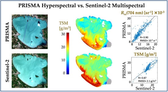
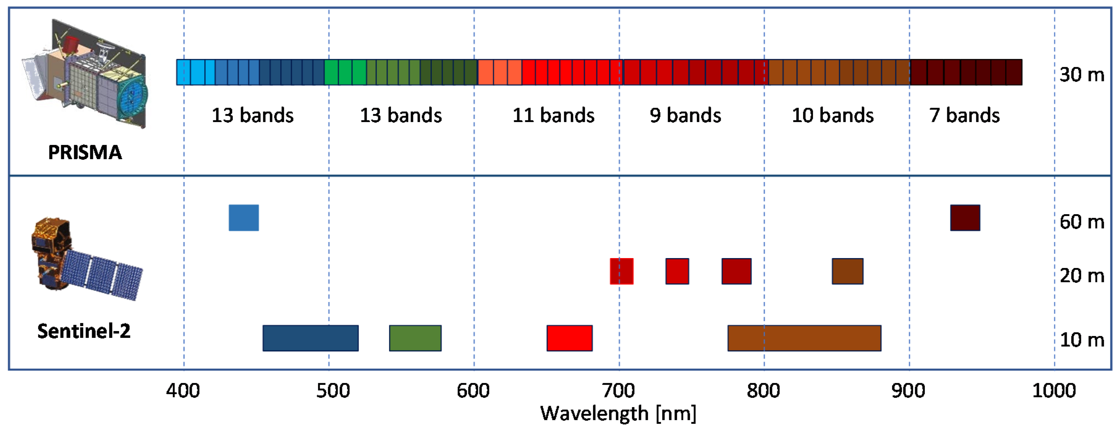
4.1. Cross-Sensor Comparison of Rrs Products

Examples of cross-sensor comparison of the Rrs spectra are shown in Figure 4 for the two stations (St1 and St2) in Lake Trasimeno (averaged within 5 × 5 windows). In both stations, the PRISMA and synthesized Sentinel-2 spectra are in good agreement with those of Sentinel-2 in terms of both shape and magnitude. However, the PRISMA-based spectra are brighter than those of Sentinel-2 within the short wavelengths (<500 nm).
We quantify the cross-sensor agreement of the entire image by performing regression analyses between PRISMA-based (synthesized Sentinel-2) and Sentinel-2 data of Rrs at different wavelengths (Figure 5, Table 3). The comparisons are made for the date that the PRISMA and Sentinel-2 acquisitions are almost simultaneous (23 April 2020 that there is a time gap of one minute and 21 s only).

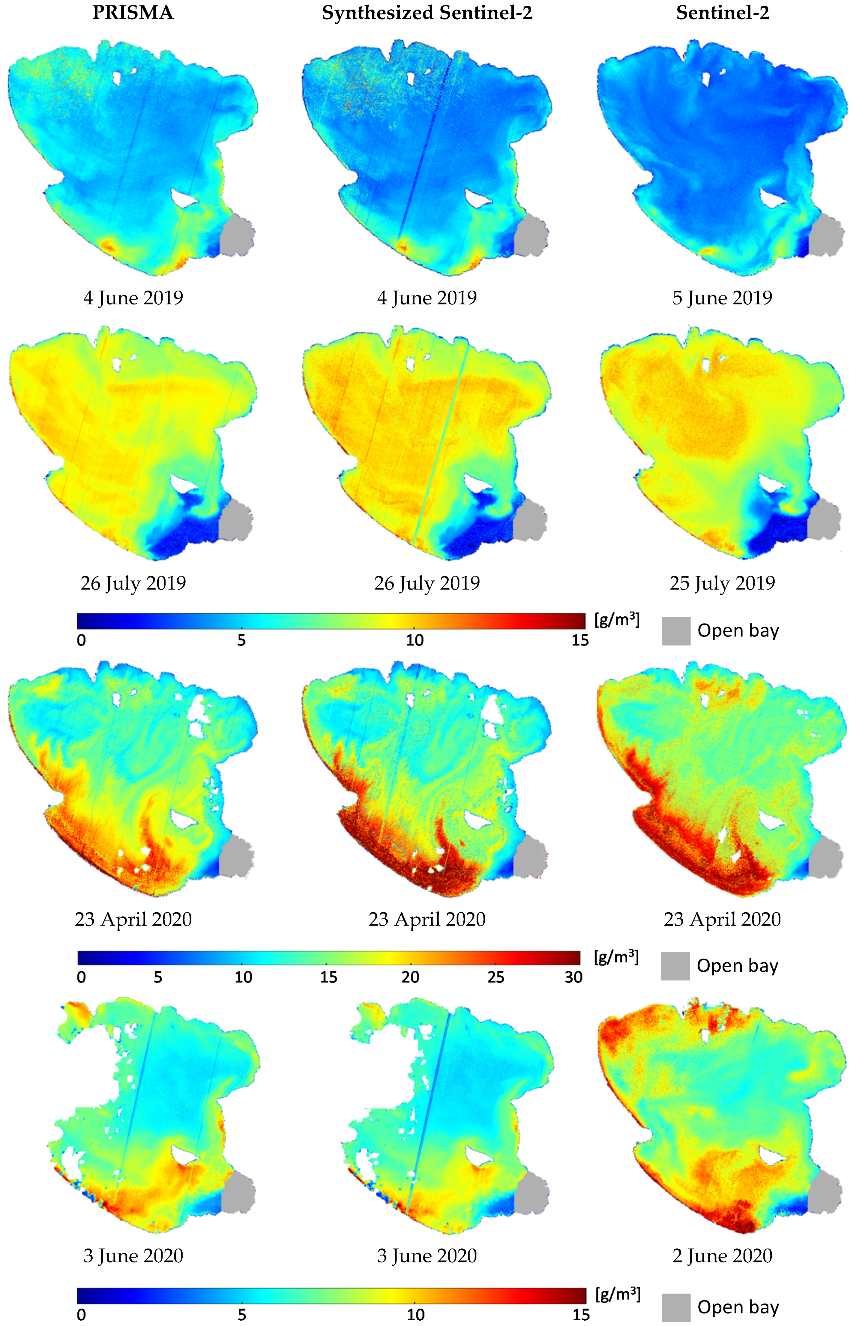
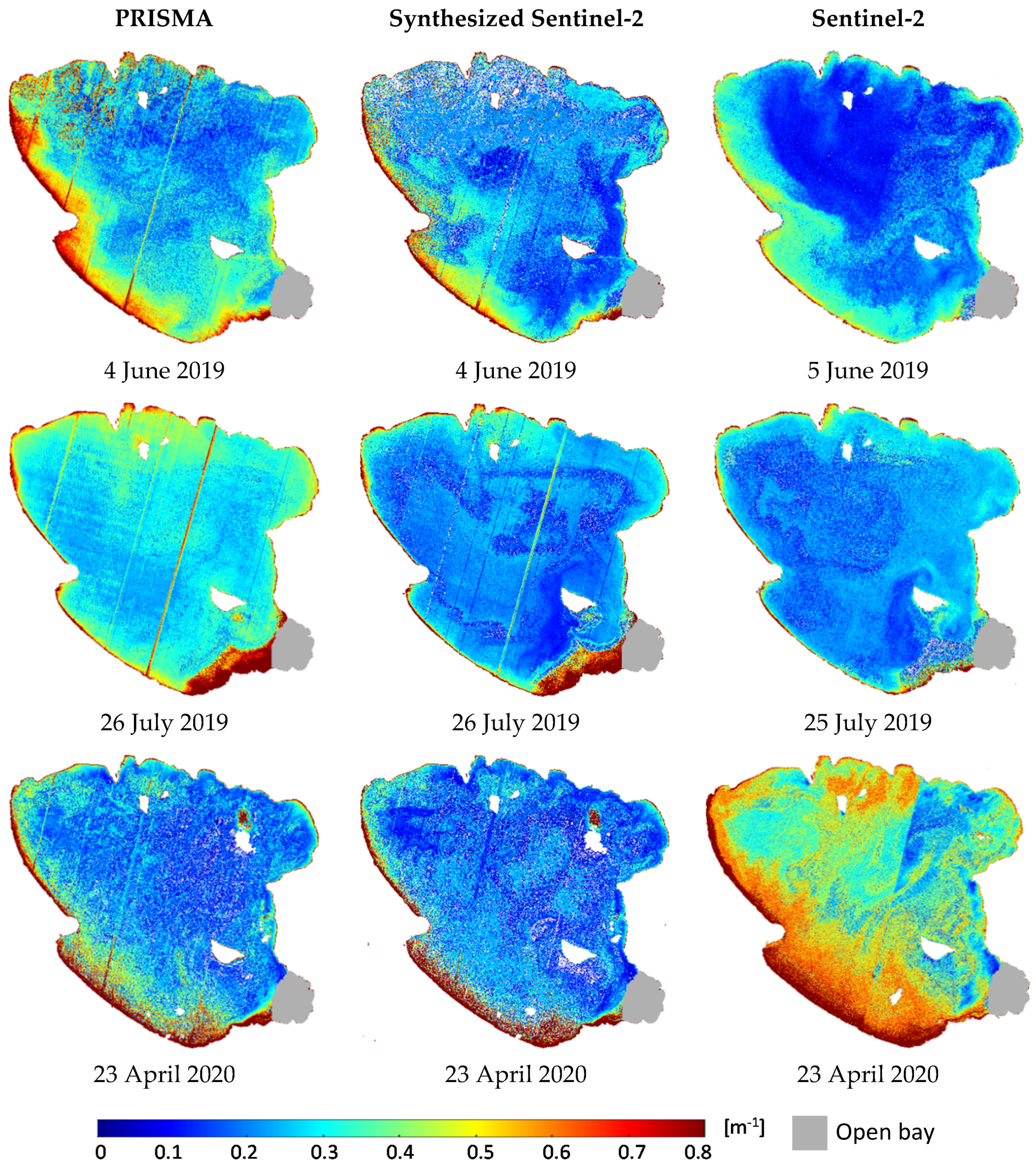
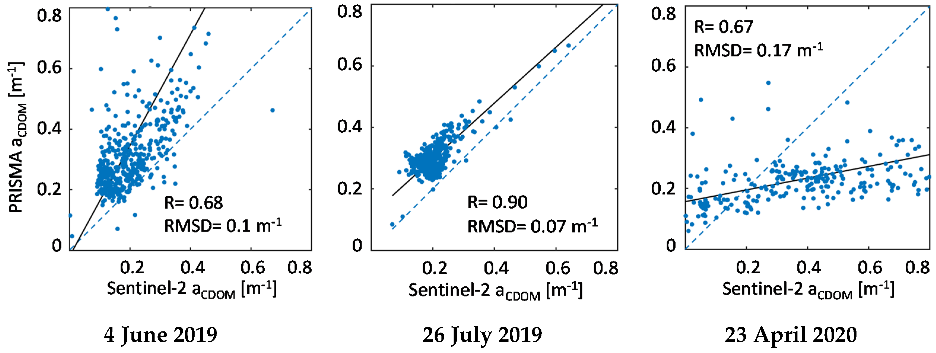
4.2. Cross-Sensor Comparison of Water Quality Products

The multitemporal TSM maps derived from PRISMA, synthesized Sentinel-2, and Sentinel-2 images are shown in Figure 6. The visual inspection of the maps conveys an intuitively good agreement among the associated TSM maps. Note that the retrievals for 23 April 2020 exhibit higher values of TSM compared to the other dates and the maps for this date are shown with a different color bar to enhance the visualization. Figure 7 and Figure 8 illustrate the retrievals of Chl-a and CDOM derived from the same images, respectively. The corresponding maps derived from PRISMA, synthesized Sentinel-2, and Sentinel-2 are in good agreement but with a lower degree compared to those of TSM.
Distribution of the retrieved constituents is investigated using boxplots in Figure 9. The bottom and top edges of boxes indicate the 25th and 75th percentiles whereas the central line and dot symbols show the median and average values, respectively. The extreme values are represented by the extensions of the boxes. These statistical indications further confirm a good cross-sensor agreement among the retrievals, particularly for TSM. The plots in Figure 9 indicate a quite high variability of the constituents over time. For instance, the PRISMA-derived average concentration of TSM on 23 April 2020 is about 2.6 times of that retrieved for 3 June 2020 (16.4 g/m3 vs. 6.2 g/m3). The multitemporal average values of TSM, Chl-a, and CDOM derived from PRISMA images are on the order of 9.1 g/m3, 4.9 mg/m3, and 0.34 m−1, respectively.
The agreements of the retrieved constituents are further examined by regressing the values extracted from the maps against each other (described in Section 3.3). The image-based matchup analyses are shown for TSM retrievals in Figure 10.
The matchup plots for Chl-a and CDOM retrievals are shown only for PRISMA vs. Sentinel-2 (Figure 11 and Figure 12) for brevity whereas the average R and RMSD values are reported in Table 4. For TSM retrievals, the average R values are 0.85, 0.97, and 0.85 with average RMSD of 1.2, 0.6, and 1.2 g/m3 for PRISMA vs. Sentinel-2, PRISMA vs. synthesized Sentinel-2, and synthesized Sentinel-2 vs. Sentinel-2, respectively. Moreover, the biases are close to unity. Note that CDOM retrievals from either PRISMA or Sentinel-2 images were not successful for June 2020 and the estimates converged to zero values for most of the pixels. This might be related to a very low (and therefore hardly detectable) concentration of CDOM. Thus, the results of CDOM retrievals for June 2020 are excluded from our analyses.
The average value of the compensating parameter for sun-glint and atmospheric artifacts ( g d d ) and the residuals of spectrum matching through the inversion ( Δ ) are reported in Table 5.

5. Discussion

According to the results, there is a strong agreement (R > 0.83) between the Rrs data derived from PRISMA and Sentinel-2. Nevertheless, the PRISMA-based Rrs at short-wavelength bands (442 nm and 492 nm) are overestimated with respect to those of Sentinel-2 (Figure 4 and Figure 5, Table 3). More agreement statistics including MAD and bias are reported in Table 3. The bias at blue bands (442 nm and 492 nm) is up to 50% (overestimation of PRISMA with respect to Sentinel-2). These short-wavelength bands are those having the most impact from the atmosphere. Thus, the cross-sensor bias in Rrs (442) and Rrs (492) data can be attributed to the differences in the atmospheric correction. The other Rrs bands show good agreement as the biases are close to unity.
The agreement statistics indicate a high consistency among the TSM retrievals from hyperspectral PRISMA and multispectral Sentinel-2 images. The agreement is also relatively strong for Chl-a and CDOM retrievals (Table 4). However, PRISMA vs. synthesized Sentinel-2 retrievals of Chl-a and CDOM are stronger (R ≈ 0.8) than when comparing with those derived from real Sentinel-2 images (R ≈ 0.7). Note that shorter wavelengths carry more information about CDOM and Chl-a than TSM particularly in turbid waters [80]. The short wavelengths are more affected by the atmosphere and thus the higher mismatches between PRISMA and Sentinel-2 derived Chl-a and CDOM can be attributed to the differences in the atmospheric corrections. The PRISMA vs. synthesized Sentinel-2 agreements are stronger than PRISMA vs. Sentinel-2 for Chl-a and CDOM. This can be attributed, to some extent, to the one-day difference between PRISMA and Sentinel-2 overpasses as the distribution and magnitude of the constituents can have some variations. The overpasses of PRISMA and Sentinel-2 are simultaneous for 23 April 2020. For this date also, PRISMA vs. Sentinel-2 agreements of Chl-a and CDOM are not as strong as those for PRISMA vs. synthesized Sentinel-2. Given the acquisitions being simultaneous (23 April 2020), the synthesized Sentinel-2 vs. Sentinel-2 differences can be related to other factors that affect all the cross-sensor comparisons: differences in the atmospheric correction, radiometric sensitivity, and SNR of PRISMA and Sentinel-2 sensors. It is worth noting that the magnitudes of the retrieved constituents are in accordance with the reported characteristics of the lake and the range of parameters (Section 2). This is an important point that the PRISMA derived water quality parameters are within the expected range for Trasimeno, which shows the potential of PRISMA for this application.
As is evident, g d d is significantly higher for PRISMA-based imagery than Sentinel-2. The high value of g d d suggests that the atmospheric path radiance is underestimated in PRISMA level 2D products. This is in line with the results derived from the cross-sensor agreement analyses among the Rrs data. As mentioned above, the agreement analyses indicated that the Rrs at short-wavelength bands (442 nm and 492 nm) of PRISMA are overestimated compared to Sentinel-2. The inversion residual based on hyperspectral PRISMA data is slightly smaller than when using multispectral Sentinel-2.

6. Conclusions and Future Work

Spaceborne hyperspectral remote sensing is an emerging area for monitoring aquatic systems, which requires a significant amount of investigation and development in terms of both methods and applications. In this study, we examined a physics-based approach for inversion of water quality parameters from the newly available hyperspectral PRISMA imagery at a turbid lake. In this context, we conducted preliminary analyses on the quality and consistency of Rrs and water quality products derived from PRISMA level 2D compared to those derived from Sentinel-2 images. The cross-sensor comparison of Rrs data showed strong agreement at different wavelengths. The cross-sensor comparison of Rrs data and gdd values suggested underestimation of path radiance for PRISMA data. The consistency analyses revealed strong agreements between synthesized Sentinel-2 imagery (PRISMA resampled) and those of PRISMA in terms of all the three types of retrieved constituents, i.e., TSM, Chl-a, and CDOM. However, the TSM products showed stronger agreement than Chl-a and CDOM. Comparing the PRISMA-derived products with those of Sentinel-2, the agreements slightly dropped for Chl-a and CDOM. This can be attributed to the differences in the atmospheric corrections of PRISMA and Sentinel-2 imagery. However, other factors such as the one-day time gap between the two satellites overpasses can, to some extent, contribute to these slight disagreements. The consistency of water quality products derived from PRISMA level 2D and Sentinel-2 is in line with the findings of the recent study [58] that demonstrated a high consistency between TOA radiance observed by the two sensors. Thus, we demonstrated the high potential of PRISMA level 2D imagery in deriving in-water constituents in a turbid lake based upon physics-based inversion modeling.
We performed the physics-based inversion using level 2D products of PRISMA which are atmospherically corrected. However, the atmospheric correction is not developed for aquatic applications. In this context, relatively large artifacts are compensated through the physics-based inversion. The development of accurate atmospheric correction methods for processing PRISMA imagery in the context of aquatic-oriented applications, particularly with leveraging the SWIR bands [63], requires specific attention in future studies. Our analyses as first experiments in processing PRISMA imagery demonstrated the high potential of this new source of spaceborne hyperspectral data in retrieving water quality parameters, though retrieval of CDOM appeared challenging. Additional studies are required to further examine the PRISMA data in the estimation of standard bio-optical properties in different aquatic environments particularly in optically shallow waters which is not addressed in this study. In future studies, the impact of noise reduction on hyperspectral PRISMA data can be investigated as a pre-processing step before applying the inversion. Moreover, the extraction of high-level products, such as the phytoplankton species and functional types, can potentially benefit from the fine and continuous spectral information offered by PRISMA. Future studies can be conducted in this direction to unlock the new opportunities of PRISMA data which can be expandable to the upcoming hyperspectral satellite missions as well.

Author Contributions

Conceptualization, M.N.-J., F.B. and L.B.; methodology, M.N.-J.; software, M.N.-J.; validation, M.N.-J.; formal analysis, M.N.-J.; investigation, M.N.-J.; resources, M.N.-J., F.B. and L.B.; data curation, M.N.-J.; writing—original draft preparation, M.N.-J.; writing—review and editing, M.N.-J., F.B. and L.B.; visualization, M.N.J.; supervision, F.B. and L.B. All authors have read and agreed to the published version of the manuscript.

Funding

This research received no external funding.

Acknowledgments

Project carried out using PRISMA Products © of the Italian Space Agency (ASI), delivered under an ASI License to use. The authors acknowledge in-situ Chl-a data provided by the regional environmental protection agency of Umbria (ARPA Umbria). We also appreciate the editor and three anonymous reviewers for their constructive comments.

Conflicts of Interest

The authors declare no conflict of interest.

References

  1. Ritchie, J.C.; Zimba, P.V.; Everitt, J.H. Remote Sensing Techniques to Assess Water Quality. Photogramm. Eng. Remote Sens. 2003, 69, 695–704. [Google Scholar] [CrossRef] [Green Version]
  2. Sheffield, J.; Wood, E.F.; Pan, M.; Beck, H.; Coccia, G.; Serrat-Capdevila, A.; Verbist, K. Satellite Remote Sensing for Water Resources Management: Potential for Supporting Sustainable Development in Data-Poor Regions. Water Resour. Res. 2018, 54, 9724–9758. [Google Scholar] [CrossRef] [Green Version]
  3. Harvey, E.T.; Kratzer, S.; Philipson, P. Satellite-based water quality monitoring for improved spatial and temporal retrieval of chlorophyll-a in coastal waters. Remote Sens. Environ. 2015, 158, 417–430. [Google Scholar] [CrossRef]
  4. Soomets, T.; Uudeberg, K.; Jakovels, D.; Zagars, M.; Reinart, A.; Brauns, A.; Kutser, T. Comparison of Lake Optical Water Types Derived from Sentinel-2 and Sentinel-3. Remote Sens. 2019, 11, 2883. [Google Scholar] [CrossRef] [Green Version]
  5. Ansper, A.; Alikas, K. Retrieval of Chlorophyll a from Sentinel-2 MSI Data for the European Union Water Framework Directive Reporting Purposes. Remote Sens. 2018, 11, 64. [Google Scholar] [CrossRef] [Green Version]
  6. Blondeau-Patissier, D.; Gower, J.F.R.; Dekker, A.G.; Phinn, S.R.; Brando, V.E. A review of ocean color remote sensing methods and statistical techniques for the detection, mapping and analysis of phytoplankton blooms in coastal and open oceans. Prog. Oceanogr. 2014, 123, 123–144. [Google Scholar] [CrossRef] [Green Version]
  7. Toming, K.; Kutser, T.; Laas, A.; Sepp, M.; Paavel, B.; Nõges, T. First Experiences in Mapping Lake Water Quality Parameters with Sentinel-2 MSI Imagery. Remote Sens. 2016, 8, 640. [Google Scholar] [CrossRef] [Green Version]
  8. Kutser, T.; Paavel, B.; Verpoorter, C.; Ligi, M.; Soomets, T.; Toming, K.; Casal, G. Remote Sensing of Black Lakes and Using 810 nm Reflectance Peak for Retrieving Water Quality Parameters of Optically Complex Waters. Remote Sens. 2016, 8, 497. [Google Scholar] [CrossRef]
  9. Bresciani, M.; Pinardi, M.; Free, G.; Luciani, G.; Ghebrehiwot, S.; Laanen, M.; Peters, S.; Della Bella, V.; Padula, R.; Giardino, C. The Use of Multisource Optical Sensors to Study Phytoplankton Spatio-Temporal Variation in a Shallow Turbid Lake. Water 2020, 12, 284. [Google Scholar] [CrossRef] [Green Version]
  10. Mishra, S.; Stumpf, R.P.; Schaeffer, B.A.; Werdell, P.J.; Loftin, K.A.; Meredith, A. Measurement of Cyanobacterial Bloom Magnitude using Satellite Remote Sensing. Sci. Rep. 2019, 9, 1–17. [Google Scholar] [CrossRef]
  11. Stumpf, R.P.; Davis, T.W.; Wynne, T.T.; Graham, J.L.; Loftin, K.A.; Johengen, T.H.; Gossiaux, D.; Palladino, D.; Burtner, A. Challenges for mapping cyanotoxin patterns from remote sensing of cyanobacteria. Harmful Algae 2016, 54, 160–173. [Google Scholar] [CrossRef] [PubMed]
  12. Soomets, T.; Uudeberg, K.; Jakovels, D.; Brauns, A.; Zagars, M.; Kutser, T. Validation and comparison of water quality products in baltic lakes using sentinel-2 msi and sentinel-3 OLCI data. Sensors 2020, 20, 742. [Google Scholar] [CrossRef] [PubMed] [Green Version]
  13. Caballero, I.; Steinmetz, F.; Navarro, G. Evaluation of the First Year of Operational Sentinel-2A Data for Retrieval of Suspended Solids in Medium- to High-Turbidity Waters. Remote Sens. 2018, 10, 982. [Google Scholar] [CrossRef] [Green Version]
  14. Kutser, T.; Pierson, D.C.; Kallio, K.Y.; Reinart, A.; Sobek, S. Mapping lake CDOM by satellite remote sensing. Remote Sens. Environ. 2005, 94, 535–540. [Google Scholar] [CrossRef]
  15. Kutser, T.; Verpoorter, C.; Paavel, B.; Tranvik, L.J. Estimating lake carbon fractions from remote sensing data. Remote Sens. Environ. 2015, 157, 138–146. [Google Scholar] [CrossRef]
  16. Slonecker, E.T.; Jones, D.K.; Pellerin, B.A. The new Landsat 8 potential for remote sensing of colored dissolved organic matter (CDOM). Mar. Pollut. Bull. 2016, 107, 518–527. [Google Scholar] [CrossRef] [PubMed]
  17. Schweizer, D.; Armstrong, R.A.; Posada, J. Remote sensing characterization of benthic habitats and submerged vegetation biomass in Los Roques Archipelago National Park, Venezuela. Int. J. Remote Sens. 2005, 26, 2657–2667. [Google Scholar] [CrossRef]
  18. Niroumand-Jadidi, M.; Pahlevan, N.; Vitti, A. Mapping Substrate Types and Compositions in Shallow Streams. Remote Sens. 2019, 11, 262. [Google Scholar] [CrossRef] [Green Version]
  19. Niroumand-Jadidi, M.; Vitti, A.; Lyzenga, D.R. Multiple Optimal Depth Predictors Analysis (MODPA) for river bathymetry: Findings from spectroradiometry, simulations, and satellite imagery. Remote Sens. Environ. 2018, 218, 132–147. [Google Scholar] [CrossRef]
  20. Lyzenga, D.R. Remote sensing of bottom reflectance and water attenuation parameters in shallow water using aircraft and Landsat data. Int. J. Remote Sens. 1981, 2, 71–82. [Google Scholar] [CrossRef]
  21. Hedley, J.D.; Roelfsema, C.; Brando, V.; Giardino, C.; Kutser, T.; Phinn, S.; Mumby, P.J.; Barrilero, O.; Laporte, J.; Koetz, B. Coral reef applications of Sentinel-2: Coverage, characteristics, bathymetry and benthic mapping with comparison to Landsat 8. Remote Sens. Environ. 2018, 216, 598–614. [Google Scholar] [CrossRef]
  22. Niroumand-Jadidi, M.; Bovolo, F.; Bruzzone, L. SMART-SDB: Sample-specific multiple band ratio technique for satellite-derived bathymetry. Remote Sens. Environ. 2020, 251, 112091. [Google Scholar] [CrossRef]
  23. Toming, K.; Kutser, T.; Uiboupin, R.; Arikas, A.; Vahter, K.; Paavel, B. Mapping Water Quality Parameters with Sentinel-3 Ocean and Land Colour Instrument imagery in the Baltic Sea. Remote Sens. 2017, 9, 1070. [Google Scholar] [CrossRef] [Green Version]
  24. Olmanson, L.G.; Brezonik, P.L.; Finlay, J.C.; Bauer, M.E. Comparison of Landsat 8 and Landsat 7 for regional measurements of CDOM and water clarity in lakes. Remote Sens. Environ. 2016, 185, 119–128. [Google Scholar] [CrossRef]
  25. Planet Imagery Product Specifications. Available online: https://assets.planet.com/docs/Planet_Combined_Imagery_Product_Specs_letter_screen.pdf (accessed on 10 July 2020).
  26. Wicaksono, P.; Lazuardi, W. Assessment of PlanetScope images for benthic habitat and seagrass species mapping in a complex optically shallow water environment. Int. J. Remote Sens. 2018, 39, 5739–5765. [Google Scholar] [CrossRef]
  27. Gabr, B.; Ahmed, M.; Marmoush, Y. PlanetScope and Landsat 8 Imageries for Bathymetry Mapping. J. Mar. Sci. Eng. 2020, 8, 143. [Google Scholar] [CrossRef] [Green Version]
  28. Niroumand-Jadidi, M.; Bovolo, F.; Bruzzone, L.; Gege, P. Physics-based Bathymetry and Water Quality Retrieval Using PlanetScope Imagery: Impacts of 2020 COVID-19 Lockdown and 2019 Extreme Flood in the Venice Lagoon. Remote Sens. 2020, 12, 2381. [Google Scholar] [CrossRef]
  29. Goetz, A.F.H. Three decades of hyperspectral remote sensing of the Earth: A personal view. Remote Sens. Environ. 2009, 113, S5–S16. [Google Scholar] [CrossRef]
  30. Transon, J.; D’Andrimont, R.; Maugnard, A.; Defourny, P. Survey of Hyperspectral Earth Observation Applications from Space in the Sentinel-2 Context. Remote Sens. 2018, 10, 157. [Google Scholar] [CrossRef] [Green Version]
  31. Gege, P.; Dekker, A.G. Spectral and Radiometric Measurement Requirements for Inland, Coastal and Reef Waters. Remote Sens. 2020, 12, 2247. [Google Scholar] [CrossRef]
  32. Guanter, L.; Kaufmann, H.; Segl, K.; Foerster, S.; Rogass, C.; Chabrillat, S.; Kuester, T.; Hollstein, A.; Rossner, G.; Chlebek, C.; et al. The EnMAP Spaceborne Imaging Spectroscopy Mission for Earth Observation. Remote Sens. 2015, 7, 8830–8857. [Google Scholar] [CrossRef] [Green Version]
  33. Ungar, S.G.; Pearlman, J.S.; Mendenhall, J.A.; Reuter, D. Overview of the Earth Observing One (EO-1) mission. IEEE Trans. Geosci. Remote Sens. 2003, 41, 1149–1159. [Google Scholar] [CrossRef]
  34. Barnsley, M.J.; Settle, J.J.; Cutter, M.A.; Lobb, D.R.; Teston, F. The PROBA/CHRIS mission: A low-cost smallsat for hyperspectral multiangle observations of the earth surface and atmosphere. IEEE Trans. Geosci. Remote Sens. 2004, 42, 1512–1520. [Google Scholar] [CrossRef]
  35. Nieke, J.; Rast, M. Towards the copernicus hyperspectral imaging mission for the environment (CHIME). In Proceedings of the International Geoscience and Remote Sensing Symposium (IGARSS), Valencia, Spain, 22–27 July 2018; pp. 157–159. [Google Scholar]
  36. Devred, E.; Turpie, K.; Moses, W.; Klemas, V.; Moisan, T.; Babin, M.; Toro-Farmer, G.; Forget, M.-H.; Jo, Y.-H. Future Retrievals of Water Column Bio-Optical Properties using the Hyperspectral Infrared Imager (HyspIRI). Remote Sens. 2013, 5, 6812–6837. [Google Scholar] [CrossRef] [Green Version]
  37. Werdell, P.J.; Behrenfeld, M.J.; Bontempi, P.S.; Boss, E.; Cairns, B.; Davis, G.T.; Franz, B.A.; Gliese, U.B.; Gorman, E.T.; Hasekamp, O.; et al. The plankton, aerosol, cloud, ocean ecosystem mission status, science, advances. Bull. Am. Meteorol. Soc. 2019, 100, 1775–1794. [Google Scholar] [CrossRef]
  38. Giardino, C.; Brando, V.E.; Gege, P.; Pinnel, N.; Hochberg, E.; Knaeps, E.; Reusen, I.; Doerffer, R.; Bresciani, M.; Braga, F.; et al. Imaging Spectrometry of Inland and Coastal Waters: State of the Art, Achievements and Perspectives. Surv. Geophys. 2019, 40, 401–429. [Google Scholar] [CrossRef] [Green Version]
  39. Vandermeulen, R.A.; Mannino, A.; Craig, S.E.; Werdell, P.J. 150 shades of green: Using the full spectrum of remote sensing reflectance to elucidate color shifts in the ocean. Remote Sens. Environ. 2020, 247, 111900. [Google Scholar] [CrossRef]
  40. Kudela, R.M.; Palacios, S.L.; Austerberry, D.C.; Accorsi, E.K.; Guild, L.S.; Torres-Perez, J. Application of hyperspectral remote sensing to cyanobacterial blooms in inland waters. Remote Sens. Environ. 2015, 167, 196–205. [Google Scholar] [CrossRef] [Green Version]
  41. Moses, W.J.; Gitelson, A.A.; Perk, R.L.; Gurlin, D.; Rundquist, D.C.; Leavitt, B.C.; Barrow, T.M.; Brakhage, P. Estimation of chlorophyll-a concentration in turbid productive waters using airborne hyperspectral data. Water Res. 2012, 46, 993–1004. [Google Scholar] [CrossRef] [Green Version]
  42. Palacios, S.L.; Kudela, R.M.; Guild, L.S.; Negrey, K.H.; Torres-Perez, J.; Broughton, J. Remote sensing of phytoplankton functional types in the coastal ocean from the HyspIRI Preparatory Flight Campaign. Remote Sens. Environ. 2015, 167, 269–280. [Google Scholar] [CrossRef]
  43. Xi, H.; Hieronymi, M.; Röttgers, R.; Krasemann, H.; Qiu, Z. Hyperspectral Differentiation of Phytoplankton Taxonomic Groups: A Comparison between Using Remote Sensing Reflectance and Absorption Spectra. Remote Sens. 2015, 7, 14781–14805. [Google Scholar] [CrossRef] [Green Version]
  44. Bell, T.W.; Cavanaugh, K.C.; Siegel, D.A. Remote monitoring of giant kelp biomass and physiological condition: An evaluation of the potential for the Hyperspectral Infrared Imager (HyspIRI) mission. Remote Sens. Environ. 2015, 167, 218–228. [Google Scholar] [CrossRef]
  45. Hu, C.; Feng, L.; Hardy, R.F.; Hochberg, E.J. Spectral and spatial requirements of remote measurements of pelagic Sargassum macroalgae. Remote Sens. Environ. 2015, 167, 229–246. [Google Scholar] [CrossRef]
  46. Giardino, C.; Brando, V.E.; Dekker, A.G.; Strömbeck, N.; Candiani, G. Assessment of water quality in Lake Garda (Italy) using Hyperion. Remote Sens. Environ. 2007, 109, 183–195. [Google Scholar] [CrossRef]
  47. Lee, Z.; Casey, B.; Arnone, R.A.; Weidemann, A.D.; Parsons, R.; Montes, M.J.; Gao, B.-C.; Goode, W.; Davis, C.O.; Dye, J. Water and bottom properties of a coastal environment derived from Hyperion data measured from the EO-1 spacecraft platform. J. Appl. Remote Sens. 2007, 1, 1–16. [Google Scholar] [CrossRef] [Green Version]
  48. Pu, R.; Bell, S. A protocol for improving mapping and assessing of seagrass abundance along the West Central Coast of Florida using Landsat TM and EO-1 ALI/Hyperion images. ISPRS J. Photogramm. Remote Sens. 2013, 83, 116–129. [Google Scholar] [CrossRef]
  49. Topp, S.N.; Pavelsky, T.M.; Jensen, D.; Simard, M.; Ross, M.R.V. Research Trends in the Use of Remote Sensing for Inland Water Quality Science: Moving Towards Multidisciplinary Applications. Water 2020, 12, 169. [Google Scholar] [CrossRef] [Green Version]
  50. PRISMA. PRISMA Products Specification. Available online: http://prisma.asi.it/missionselect/docs/PRISMA%20Product%20Specifications_Is2_3.pdf (accessed on 4 August 2020).
  51. Mobley, C.D. Light and Water: Radiative Transfer in Natural Waters; Academic Press: Cambridge, MA, USA, 1994; ISBN 9780125027502. [Google Scholar]
  52. Gege, P. The water color simulator WASI: An integrating software tool for analysis and simulation of optical in situ spectra. Comput. Geosci. 2004, 30, 523–532. [Google Scholar] [CrossRef]
  53. Brando, V.E.; Anstee, J.M.; Wettle, M.; Dekker, A.G.; Phinn, S.R.; Roelfsema, C. A physics based retrieval and quality assessment of bathymetry from suboptimal hyperspectral data. Remote Sens. Environ. 2009, 113, 755–770. [Google Scholar] [CrossRef]
  54. Niroumand-Jadidi, M.; Vitti, A. Optimal band ratio analysis of WorldView-3 imagery for bathymetry of shallow rivers (case study: Sarca River, Italy). In International Archives of the Photogrammetry, Remote Sensing and Spatial Information Sciences—ISPRS Archives; ISPRS: Prague, Czech Republic, 2016; Volume 41. [Google Scholar]
  55. Niroumand-Jadidi, M.; Bovolo, F.; Vitti, A.; Bruzzone, L. A novel approach for bathymetry of shallow rivers based on spectral magnitude and shape predictors using stepwise regression. In Proceedings of the Image and Signal Processing for Remote Sensing XXIV, Berlin, Germany, 10–12 September 2018; Bruzzone, L., Bovolo, F., Benediktsson, J.A., Eds.; SPIE: Bellingham, WA, USA, 2018; Volume 10789, p. 23. [Google Scholar]
  56. Niroumand-Jadidi, M.; Bovolo, F.; Bruzzone, L. Novel Spectra-Derived Features for Empirical Retrieval of Water Quality Parameters: Demonstrations for OLI, MSI, and OLCI Sensors. IEEE Trans. Geosci. Remote Sens. 2019, 57, 10285–10300. [Google Scholar] [CrossRef]
  57. Niroumand-Jadidi, M.; Vitti, A. Reconstruction of river boundaries at sub-pixel resolution: Estimation and spatial allocation of water fractions. ISPRS Int. J. Geo-Inf. 2017, 6, 383. [Google Scholar] [CrossRef] [Green Version]
  58. Giardino, C.; Bresciani, M.; Braga, F.; Fabbretto, A.; Ghirardi, N.; Pepe, M.; Gianinetto, M.; Colombo, R.; Cogliati, S.; Ghebrehiwot, S.; et al. First Evaluation of PRISMA Level 1 Data for Water Applications. Sensors 2020, 20, 4553. [Google Scholar] [CrossRef] [PubMed]
  59. Gege, P. WASI-2D: A software tool for regionally optimized analysis of imaging spectrometer data from deep and shallow waters. Comput. Geosci. 2014, 62, 208–215. [Google Scholar] [CrossRef] [Green Version]
  60. Gege, P. Chapter 2—Radiative Transfer Theory for Inland Waters. In Bio-Optical Modeling and Remote Sensing of Inland Waters; Mishra, D.R., Ogashawara, I., Gitelson, A.A., Eds.; Elsevier: Amsterdam, The Netherlands, 2017; pp. 25–67. ISBN 978-0-12-804644-9. [Google Scholar]
  61. Dörnhöfer, K.; Göritz, A.; Gege, P.; Pflug, B.; Oppelt, N. Water Constituents and Water Depth Retrieval from Sentinel-2A—A First Evaluation in an Oligotrophic Lake. Remote Sens. 2016, 8, 941. [Google Scholar] [CrossRef] [Green Version]
  62. Giardino, C.; Bresciani, M.; Valentini, E.; Gasperini, L.; Bolpagni, R.; Brando, V.E. Airborne hyperspectral data to assess suspended particulate matter and aquatic vegetation in a shallow and turbid lake. Remote Sens. Environ. 2015, 157, 48–57. [Google Scholar] [CrossRef]
  63. Vanhellemont, Q.; Ruddick, K. Advantages of high quality SWIR bands for ocean colour processing: Examples from Landsat-8. Remote Sens. Environ. 2015, 161, 89–106. [Google Scholar] [CrossRef] [Green Version]
  64. Pereira-Sandoval, M.; Ruescas, A.; Urrego, P.; Ruiz-Verdú, A.; Delegido, J.; Tenjo, C.; Soria-Perpinyà, X.; Vicente, E.; Soria, J.; Moreno, J. Evaluation of Atmospheric Correction Algorithms over Spanish Inland Waters for Sentinel-2 Multi Spectral Imagery Data. Remote Sens. 2019, 11, 1469. [Google Scholar] [CrossRef] [Green Version]
  65. Warren, M.A.; Simis, S.G.H.; Martinez-Vicente, V.; Poser, K.; Bresciani, M.; Alikas, K.; Spyrakos, E.; Giardino, C.; Ansper, A. Assessment of atmospheric correction algorithms for the Sentinel-2A MultiSpectral Imager over coastal and inland waters. Remote Sens. Environ. 2019, 225, 267–289. [Google Scholar] [CrossRef]
  66. Kyryliuk, D.; Kratzer, S. Evaluation of Sentinel-3A OLCI Products Derived Using the Case-2 Regional CoastColour Processor over the Baltic Sea. Sensors 2019, 19, 3609. [Google Scholar] [CrossRef] [Green Version]
  67. Buraschi, E.; Buzzi, F.; Garibaldi, L.; Lugliè, A.; Legnani, E.; Morabito, G.; Oggioni, A.; Pozzi, S.; Salmaso, N.; Gianni, T. Protocollo Per il Campionamento di Fitoplancton in Ambiente Lacustre. Available online: https://www.researchgate.net/publication/270273561_Protocollo_per_il_campionamento_di_fitoplancton_in_ambiente_lacustre (accessed on 4 November 2020).
  68. APAT Metodi Analitici Per le Acque. Available online: https://www.isprambiente.gov.it/it/pubblicazioni/manuali-e-linee-guida/metodi-analitici-per-le-acque (accessed on 4 November 2020).
  69. Albert, A.; Mobley, C. An analytical model for subsurface irradiance and remote sensing reflectance in deep and shallow case-2 waters. Opt. Express 2003, 11, 2873. [Google Scholar] [CrossRef]
  70. Albert, A. Inversion Technique for Optical Remote Sensing in Shallow Water; University of Hamburg: Hamburg, Germany, 2004. [Google Scholar]
  71. Pope, R.M.; Fry, E.S. Absorption spectrum (380–700 nm) of pure water II Integrating cavity measurements. Appl. Opt. 1997, 36, 8710. [Google Scholar] [CrossRef] [PubMed]
  72. Kou, L.; Labrie, D.; Chylek, P. Refractive indices of water and ice in the 065- to 25-μm spectral range. Appl. Opt. 1993, 32, 3531. [Google Scholar] [CrossRef] [PubMed] [Green Version]
  73. Morel, A. Optical Properties of Pure Water and Pure Sea Water. Opt. Asp. Oceanogr. 1974, 14, 1–24. [Google Scholar]
  74. Gege, P.; Groetsch, P. A spectral model for correcting sun glint and sky glint. In Proceedings of the Ocean Optics XXIII, Victoria, BC, Canada, 23–28 October 2016. [Google Scholar]
  75. Jerlov, N.G. Marine Optics; Elsevier Scientific Publisher Company: Amsterdam, The Netherlands, 1976. [Google Scholar]
  76. Gege, P. Analytic model for the direct and diffuse components of downwelling spectral irradiance in water. Appl. Opt. 2012, 51, 1407–1419. [Google Scholar] [CrossRef] [PubMed] [Green Version]
  77. Gregg, W.W.; Carder, K.L. A simple spectral solar irradiance model for cloudless maritime atmospheres. Limnol. Oceanogr. 1990, 35, 1657–1675. [Google Scholar] [CrossRef]
  78. Gege, P. WASI (Water Colour Simulator). Available online: www.ioccg.org/data/software.html (accessed on 20 November 2020).
  79. Seegers, B.N.; Stumpf, R.P.; Schaeffer, B.A.; Loftin, K.A.; Werdell, P.J. Performance metrics for the assessment of satellite data products: An ocean color case study. Opt. Express 2018, 26, 7404. [Google Scholar] [CrossRef] [Green Version]
  80. Gholizadeh, M.H.; Melesse, A.M.; Reddi, L. A Comprehensive Review on Water Quality Parameters Estimation Using Remote Sensing Techniques. Sensors 2016, 16, 1298. [Google Scholar] [CrossRef] [Green Version]
Figure 1. True color images of Lake Trasimeno (a) PRecursore IperSpettrale della Missione Applicativa (PRISMA) (641.55 nm, 546.66 nm, 471.12, nm), (b) PRISMA resampled to Sentinel-2B (664.9 nm, 559 nm, 492.1 nm), and (c) Sentinel-2B (664.9 nm, 559 nm, 492.1 nm) acquired on 23 April 2020. The in-situ stations (St1, St2) are located on the left image. The open bay colonized by aquatic vegetation is highlighted by a red box [9].
Remotesensing 12 03984 g001
Figure 2. Thematic representation of the PRISMA and Sentinel-2 spectral bands and spatial resolutions.
Remotesensing 12 03984 g002
Figure 3. The specific absorption spectrum of phytoplankton a p h y * ( λ ) measured in Lake Trasimeno [62].
Remotesensing 12 03984 g003
Figure 4. Rrs spectra for the stations St1 (a) and St2 (b) in Lake Trasimeno based on PRISMA and Sentinel-2 acquisitions on 23 April 2020.
Remotesensing 12 03984 g004
Figure 5. Cross-sensor agreement analyses between the Rrs data derived from PRISMA (resampled to Sentinel-2 bands) and Sentinel-2 (acquired on 23 April 2020).
Remotesensing 12 03984 g005
Figure 6. Multitemporal total suspended matter (TSM) maps derived from PRISMA, synthesized Sentinel-2 (PRISMA resampled), and Sentinel-2 images. The missing data are related to the cloud cover.
Remotesensing 12 03984 g006
Figure 7. Multitemporal Chl-a maps derived from PRISMA, synthesized Sentinel-2 (PRISMA resampled), and Sentinel-2 images. The missing data are related to the cloud cover.
Remotesensing 12 03984 g007
Figure 8. Multitemporal CDOM maps derived from PRISMA, synthesized Sentinel-2 (PRISMA resampled), and Sentinel-2 images.
Remotesensing 12 03984 g008
Figure 9. Distribution of the retrieved constituents (TSM, Chl-a, and CDOM) from PRISMA, synthesized Sentinel-2 (PRISMA resampled), and Sentinel-2 images.
Remotesensing 12 03984 g009
Figure 10. Agreement analyses among the TSM derived from PRISMA, synthesized Sentinel-2 (PRISMA resampled), and Sentinel-2 images in terms of R and RMSD.
Remotesensing 12 03984 g010
Figure 11. Agreement analyses among the Chl-a derived from PRISMA and Sentinel-2 images in terms of R and RMSD.
Remotesensing 12 03984 g011
Figure 12. Agreement analyses among the CDOM derived from PRISMA and Sentinel-2 images in terms of R and RMSD.
Remotesensing 12 03984 g012
Table 1. PRISMA and Sentinel-2 acquisitions over Lake Trasimeno.
PRISMA4 June 201926 July 201923 April 20203 June 2020
Sentinel-25 June 201925 July 201923 April 20202 June 2020
Table 2. Fit parameters and associated initial values for water quality inversion using Water Color Simulator (WASI).
Fit ParameterInitial ValueMinMaxUnitsDescription
C N A P 70100g m−3Concentration of NAP
C p h y 501000mg m−3Concentration of phytoplankton
a C D O M ( 440 ) 0.2050m−1Absorption coefficient of CDOM at 440 nm
g d d 0.02−110sr−1Fraction of sky radiance due to direct solar radiation
Table 3. The agreement statistics for the cross-sensor comparison of Rrs at different wavelengths derived from PRISMA and Sentinel-2 data.
442 nm492 nm559 nm664 nm704 nm740 nm781 nm864 nm
R0.830.840.910.890.900.880.870.88
RMSD (sr−1)4 × 10−37 × 10−310−32 × 10−310−36 × 10−38 × 10−34 × 10−3
MAD1.511.531.041.131.091.181.191.42
Bias1.511.531.031.121.060.961.130.83
Table 4. The agreement analyses among the retrieved constituents in terms of average R and RMSD.
PRISMA vs. Sentinel-2PRISMA vs. Synthesized Sentinel-2Synthesized Sentinel-2 vs. Sentinel-2
RRMSDMADBiasRRMSDMADBiasRRMSDMADBias
TSM84.81.2 g/m31.261.1297.50.6 g/m31.181.0584.81.2 g/m31.211.09
Chl-a64.51.2 mg/m31.390.8384.60.8 mg/m31.310.8167.31.3 mg/m31.270.93
CDOM75.00.11 m−11.321.2485.90.05 m−11.261.1776.10.13 m−11.191.08
Table 5. Average g d d and Δ derived through the inversion.
PRISMASynthesized Sentinel-2Sentinel-2
g d d (sr−1)0.260.250.04
Δ (sr−2)1.4 × 10−42.4 × 10−41.9 × 10⁻⁴
Publisher’s Note: MDPI stays neutral with regard to jurisdictional claims in published maps and institutional affiliations.

