Article

Application of Lithological Mapping Based on Advanced Hyperspectral Imager (AHSI) Imagery Onboard Gaofen-5 (GF-5) Satellite

1
School of Earth Sciences and Resources, China University of Geosciences, Beijing 100083, China
2
State Key Lab of Geological Processes and Mineral Resources, China University of Geosciences, Beijing 100083, China
*
Author to whom correspondence should be addressed.
Remote Sens. 2020, 12(23), 3990; https://0-doi-org.brum.beds.ac.uk/10.3390/rs12233990
Submission received: 24 October 2020 / Revised: 2 December 2020 / Accepted: 3 December 2020 / Published: 6 December 2020

Abstract

:
The Advanced Hyperspectral Imager (AHSI), carried by the Gaofen-5 (GF-5) satellite, is the first hyperspectral sensor that simultaneously offers broad coverage and a broad spectrum. Meanwhile, deep-learning-based approaches are emerging to manage the growing volume of data produced by satellites. However, the application potential of GF-5 AHSI imagery in lithological mapping using deep-learning-based methods is currently unknown. This paper assessed GF-5 AHSI imagery for lithological mapping in comparison with Shortwave Infrared Airborne Spectrographic Imager (SASI) data. A multi-scale 3D deep convolutional neural network (M3D-DCNN), a hybrid spectral CNN (HybridSN), and a spectral–spatial unified network (SSUN) were selected to verify the applicability and stability of deep-learning-based methods through comparison with support vector machine (SVM) based on six datasets constructed by GF-5 AHSI, Sentinel-2A, and SASI imagery. The results show that all methods produce classification results with accuracy greater than 90% on all datasets, and M3D-DCNN is both more accurate and more stable. It can produce especially encouraging results by just using the short-wave infrared wavelength subset (SWIR bands) of GF-5 AHSI data. Accordingly, GF-5 AHSI imagery could provide impressive results and its SWIR bands have a high signal-to-noise ratio (SNR), which meets the requirements of large-scale and large-area lithological mapping. And M3D-DCNN method is recommended for use in lithological mapping based on GF-5 AHSI hyperspectral data.

Graphical Abstract

1. Introduction

Lithological mapping using remote sensing data is one of the most challenging tasks in geological remote sensing given complexities involving sub-pixel-level microscopic-scale non-linear mixing of minerals and the presence of surface soil, regolith, and vegetation [1]. Hyperspectral technology combines two-dimensional imaging and spectroscopy technologies to obtain both the physiographic and spectral information of the constituent features [2]. Compared with multispectral imagery, more diagnostic absorption features of ground objects are recorded in hyperspectral imagery (HSI), so specific minerals and litho-units could be identified and classified more accurately, which happens to be a main force driving the application and development of hyperspectral technology in the geological field.
The advent of Hyperion onboard the Earth Observing-1 (EO-1) spacecraft marked the beginning of the application of spaceborne hyperspectral data in geology [3]. Since its launch in 2000, the Hyperion sensor was in service for more than a decade, but it provided bad data lines and vertical stripes, low signal-to-noise ratio (SNR; especially the short-wave infrared bands), and poor data quality [4]. As EO-1 was a tasking satellite, it collected data only when requested, which means it did not provide continuous coverage of the Earth. Moreover, the EO-1 satellite was decommissioned on 22 February 2017 [5]. The imagery of some other airborne hyperspectral sensors are also fully applied in geological fields, such as Airborne Visible/Infrared Imaging Spectrometer (AVIRIS) [6,7], HyMap [8,9], Compact Airborne Spectrographic Imager/Shortwave infrared Airborne Spectrographic Imager (CASI/SASI) [10], Multispectral Infrared Visible Imaging Spectrometer (MIVIS) [11,12], etc. However, the acquisition of airborne high-resolution hyperspectral imagery is expensive, and the coverage of the data is limited. Fortunately, Advanced Hyperspectral Imager (AHSI), carried by the Gaofen-5 (GF-5) satellite launched on 9 May 2018, is the first hyperspectral sensor that simultaneously provides broad coverage and a broad spectrum [13,14], providing a new data source for surface research. Currently, no relevant research has been conducted on GF-5 AHSI hyperspectral imagery in lithological mapping.
In terms of lithological and mineral mapping, a large number of methods based on hyperspectral imagery have been proposed, which can be mainly divided into three categories: whole-pixel classification approaches, subpixel classification approaches, and machine-learning and deep-learning-based techniques [1,15]. Whole-pixel classification approaches assign an entire pixel to a single class based on features such as spectral similarity measures and derivative absorption band parameters. Spectral Angle Mapper (SAM) [16,17], cross-correlogram spectral matching technique (CCSM) [18], spectral information divergence (SID) [19], and spectral feature fitting (SFF) approach [20] are the most commonly used techniques. Alternatively to these methods relying on spectral reference libraries, the relative intensity and wavelength position of diagnostic absorption features can be extracted from the hyperspectral reflectance spectra to discriminate mineral species and lithologies [21,22]. Subpixel classification approaches comprise some techniques to unmix hyperspectral imagery to quantify the relative abundance of various materials within a pixel and assign a label to the pixel into a single or multiple classes depending on the purity of the pixel [15]. For instance, a typical mineral mapping process based on hyperspectral imagery has been formed by Minimum Noise Fraction (MNF), Pixel Purity Index (PPI), N-dimensional visualization, endmember selection, and mineral mapping techniques (such as SAM and SFF) [3,23].
Machine-learning-based approaches for unmixing mineral groups and lithologies from hyperspectral imagery have been thoroughly developed in the literature. For instance, support vector machine (SVM) [24,25] and random forest (RF) [26,27] are among the most widely used classifiers for classification based on HSI, which categorize pixels according to spectral similarity between the test and training samples [28]. Deep learning structures have attained success due to their outstanding generalization capacity. Various atmospheric scattering conditions, complicated light-scattering mechanisms, interclass similarity, and intraclass variability result in the hyperspectral imaging procedure being inherently nonlinear [29]. Compared to the previously mentioned shallow models, deep learning architectures are able to extract high-level, hierarchical, and abstract features, which are generally more robust to nonlinear processing. Many studies have proved that compared with traditional machine learning classification algorithms, these deep learning classification models, such as stacked autoencoder (SAE) [30], deep belief network (DBN) [31], and convolutional neural network (CNN) [32,33], can achieve more accurate classification results, but they have shortcomings. With the SAE and DBN algorithms, the original image patches must be flattened into the form of column vectors to meet the needs of their specific networks [34], which would destroy the original data structure, causing the critical information between spatial categories to be severely damaged, affecting the final classification results. Thankfully, the CNN input is the original image patches, without any deformation of the image data, so CNN can learn more complete feature information. In recent years, CNN has gradually shown its significant advantages of lithological recognition and mapping on diverse data sources [35,36,37]. However, the convolution kernel commonly used in CNN is usually two-dimensional. Although most spatial information is extracted, the spectral information is not fully used.
Extracting and integrating the spatial distribution features and spectral information in a deep learning framework has been attempted in a number of new studies. 3D-CNN was proposed to extract effective spectral–spatial features of hyperspectral imagery, but it has problems with over-fitting and increased computational complexity [32]. A multi-scale 3D deep convolutional neural network (M3D-DCNN) was proposed for HSI classification, which could jointly learn both 2D multi-scale spatial feature and 1D spectral feature from HSI data in an end-to-end approach [38]. Zhao and Du proposed a spectral–spatial feature-based classification (SSFC) framework that jointly uses dimension reduction and deep learning techniques to extract spectral and spatial features, respectively, which are then combined and fed into the SVM or logistic regression classifier [39]. Based on the above network structure, to overcome the limitation of feature extraction and classifier training not using a unified objective function, the spectral–spatial unified network (SSUN) was proposed, combining the long short-term memory (LSTM) model and a multiscale CNN (MSCNN) model for spectral feature and spatial information extraction, respectively [34]. A hybrid spectral CNN (HybridSN) was proposed with a spectral–spatial 3D-CNN followed by spatial 2D-CNN [40]. The above methods produced satisfactory results on the public benchmark datasets, such as Indian Pines, Pavia Centre and University, Salinas, etc., which mainly include land cover and land use types with uniform scale, regular shape, and clear texture feature. However, due to the complexity and multistage nature of geological processes, whether these methods are suitable for lithological mapping based on GF-5 AHSI imagery remains to be further studied.
Therefore, we used deep-learning-based techniques to perform lithological mapping based on six diverse datasets constructed by GF-5 AHSI, Sentinel-2A, and SASI imagery, mainly for two purposes: (1) to assess the suitability of GF-5 AHSI imagery for lithological mapping and (2) to verify the applicability and stability of the above deep-learning-based techniques in lithological mapping.
The rest of this paper is organized as follows: Section 2 introduces the location and geological background of the study area. Section 3 describes datasets and methods. Section 4 presents the experimental results. Discussion is provided in Section 5 and our conclusions are summarized in Section 6.

2. Study Area

To verify the developed deep-learning-based methods and GF-5 AHSI imagery in lithological mapping, part of the area near Liuyuan town in northwest Gansu province, China, was selected as a geological test site, which covered an area of about 40 km2 (Figure 1). It is a shallow-cut mountainous area with an average altitude of about 1800 m and a typical continental-semi-desert climate. Except for sudden floods in the rainy season, there is no regular surface runoff. It is windy all year round, and wind erosion and transport are strong. Most of the bedrock is fully exposed [10].
Geologically, the study area is mostly covered with litho-units from Quaternary strata, Ordovician Huaniushan strata, and Sinian Xichangjing strata, and is heavily invaded by intermediate-acid magmatic rocks. Quaternary strata are concentrated in the northern part of the study area, and the main litho-unit is diluvial gravel and sand. Ordovician Huaniushan strata [41] are distributed in the south of the study area and spread in an east-west direction. It can be divided into lower, middle, and upper rock groups. The lower rock group is characterized by hornstone and slate; the middle rock group is dominated by basalt with slate; and the main litho-units of the upper group are hornstone and sandstone. Sinian Xichangjing strata [42] are divided into six groups from old to young, and the main litho-units are slate and phyllite, marble with phyllite, limestone, hornstone, slate, and biotite felsic slate, respectively. Besides, the majorly representative intrusive rocks are variscan diorite, variscan granodiorite, indosinian granite, and indosinian biotite granite, which account for about 40% of the whole study area and are produced in the form of batholith, stock, and dykes.
There are few faults in the study area, but from the perspective of the large-scale area, faults are developed with the largest scale in the near EW direction, followed by NE and NW directions. Liuyuan town is rich in economic minerals such as gold, silver, lead, zinc, tungsten, etc. [41].

3. Materials and Methods

3.1. Data Sources

Gaofen-5 (GF-5) Advanced Hyperspectral Imager (AHSI) imagery, Shortwave Infrared Airborne Spectrographic Imager (SASI) imagery, and Sentinel-2A imagery were used in this study. In addition, regional geological map and related explanatory materials were also obtained.

3.1.1. GF-5 AHSI Imagery

GF-5 is the fifth satellite of a series of the China High-Resolution Earth Observation System (CHEOS) satellites of the China National Space Administration (CNSA). The satellite carries 6 payloads: 2 hyperspectral/multispectral payloads for terrestrial Earth observation and 4 atmospheric observation payloads [14]. The specifications and major orbit parameters of the GF-5 satellite are shown in Table 1.
AHSI imagery (GF5_AHSI_E95.58_N41.19_20191010_007564_L10000062261) was adopted in this study, which was obtained from Land Satellite Remote Sensing Application Center of Ministry of Natural Resources, China. And High-resolution Earth observation system grid platform is available for ordering GF-5 AHSI data (https://www.cheosgrid.org.cn/index.htm). AHSI is a 330-channel imaging spectrometer with an approximately 30 m spatial resolution covering the 0.4–2.5 μm spectral range [43]. The AHSI data was acquired at 06:32:21 on 10 October 2019, and the central location has a longitude of 95.58° E and a latitude of 41.19° N. The quality of digital remote sensing data is directly related to the level of system noise relative to signal strength, which is usually expressed as signal-to-noise ratio (SNR), a dimensionless number that describes the overall system radiometric performance [44]. The visible and near-infrared (VNIR) SNR of AHSI data is nearly 700, whereas the shortwave infrared (SWIR) SNR can be close to 500 (Figure 2) [45], which is significantly higher than Hyperion imagery. The parameters of GF-5 AHSI and Hyperion are compared in Table 2. However, the Hyperion imagery does not cover the study area.

3.1.2. SASI Imagery

To verify the applicability of the short-wave infrared wavelength subset (SWIR bands) of GF-5 AHSI imagery in lithological mapping, Shortwave Infrared Airborne Spectrographic Imager (SASI) hyperspectral imagery was used for comparative analysis, which was provided by Beijing Research Institute of Uranium Geology (Beijing, China). SASI is the advanced hyperspectral imaging spectrometer in the world, known as the SASI-600 sensor, which is produced by the Canadian company ITRES; it is characterized by high spatial resolution and high spectral resolution. The spectral range of SASI is 950–2450 nm, and the specific technical indexes of SASI are shown in Table 3 [42]. The scanner flew over the study area at a relative height of about 2000 m on 7 September 2010, between 14:00 and 16:30, and five lines of data were acquired during the overpasses. The SASI data is not publicly available, and readers can contact authors for some sample data.

3.1.3. Sentinel-2A Imagery

Sentinel-2 is a multi-spectral mission consisting of a pair of optical Earth observation satellites: Sentinel-2A (S2A) and Sentinel-2B (S2B), operated by the European Space Agency (ESA) within the framework of the Copernicus program [46]. Each Sentinel-2 satellite carries a single multi-spectral instrument (MSI) that uses a push-broom concept and provides 13 spectral channels ranging from the visible (VIS) to the short-wavelength infrared (SWIR) at different spatial resolutions (10, 20, and 60 m) [47,48]. In this study, we downloaded the S2A level-1C product (S2A_MSIL1C_20191019T042801_N0208_R133_T46TGL_20191019T071843.SAFE) from the ESA Copernicus Open Access Hub (https://scihub.copernicus.eu/) [49], which provides unlimited open access to the Sentinel-2 Level-1C (L1C) user products. The S2A imagery was acquired at 04:28:01 on 19 October 2019, and the longitude and latitude of the central location are 96.03° E and 41.02° N respectively.

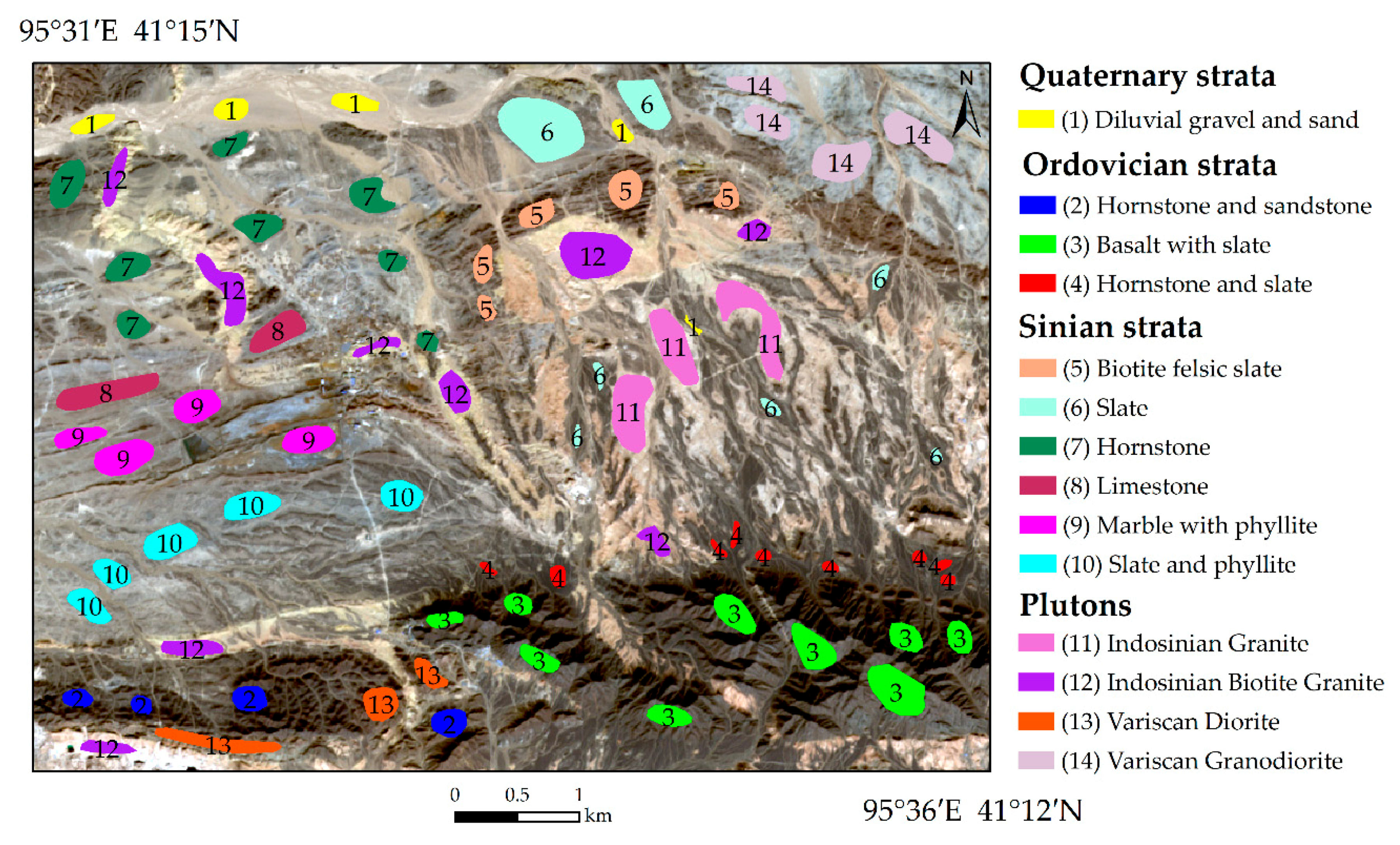
3.1.4. Geological Map

Regional geological map and related explanatory materials were provided by China Aero Geophysical Survey and Remote Sensing Center (AGRS). And GeoCloud of China Geological Survey is available for ordering geological data (http://geocloud.cgs.gov.cn/#/portal/home). The geological map at a scale of 1:50,000 was created in 2016. In this paper, a local-scale geological map of the study area (Figure 1), based on the initial geological map, updated with GF-5 AHSI, S2A, and SASI data by visual interpretation. And this map would serve as an important reference for further research.

3.2. Data Pre-Processing

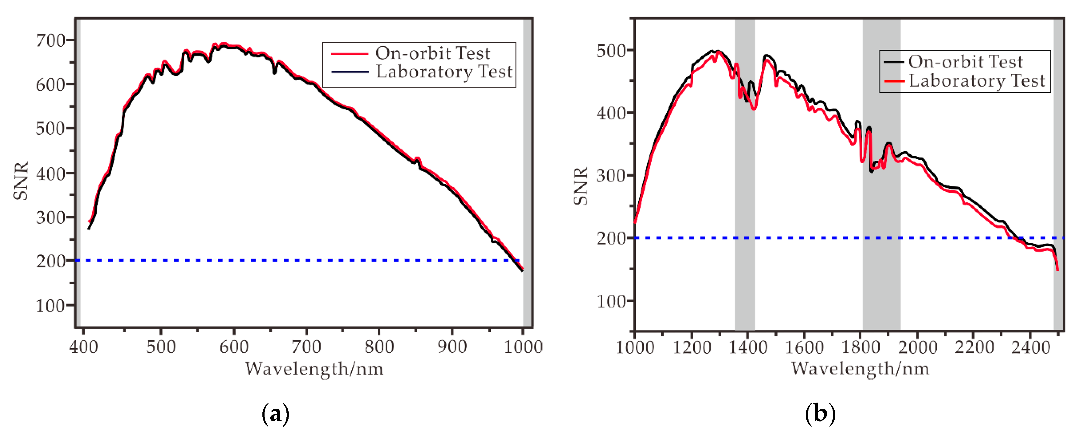
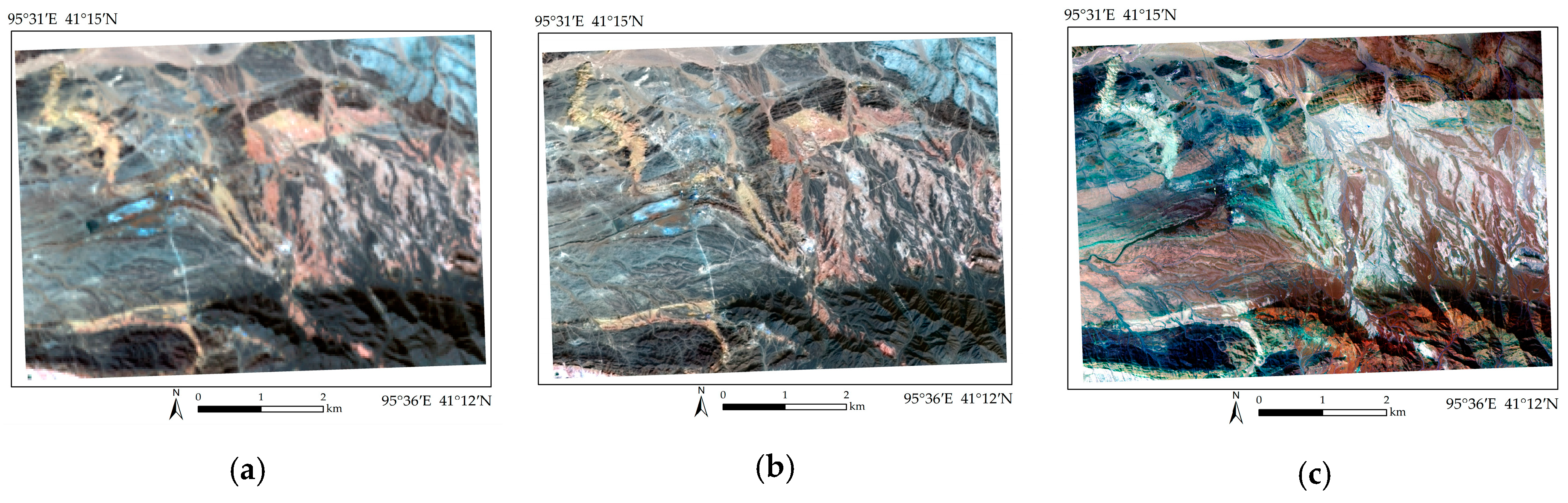
3.2.1. Pre-Processing of GF-5 AHSI Imagery

The GF-5 AHSI imagery used in this study are laboratory level-1 data, which means that it had already undergone systematic radiometric calibration and geometric correction with the GCS_WGS_1984 coordinate system. The pre-processing of GF-5 AHSI imagery mainly included six steps: (1) band removal, (2) radiometric calibration, (3) bad lines repair and stripe removal, (4) atmospheric correction, (5) reduce noise by minimum noise fraction (MNF) rotation, and (6) subset data from study area. The pre-processing of GF-5 AHSI imagery was completed on ENVI5.3 + IDL8.5 software (Harris Geospatial Solutions, Inc., Broomfield, CO, USA).
(1) Band Removal. The spectral resolution of GF-5 AHSI’s VNIR bands and SWIR bands are approximately 5 and 10 nm, respectively. It contains a total of 330 bands with level-1 data, among which only 305 bands are calibrated (1–150 for VNIR, and 151–192, 201–245, and 263–330 for SWIR), and the other 25 bands (193–200 and 246–262 from the SWIR) have poor signal due to their detector’s low responsivity. VNIR and SWIR bands overlap between bands 144–150 and 151–153. Due to a higher SNR (Figure 2) and more direct comparative analysis with SASI data, bands 151–153 were retained. Noisy bands due to atmospheric water absorption (bands 1–2 and 327–330) were removed, so only the remaining 292 bands were used for further study (Figure 2).
(2) Radiometric Calibration. Radiometric calibration was applied to GF-5 AHSI imagery to calibrate image data to radiance and selected band interleaved by line (BIL) as the output interleave. Scale factor was set to 0.10, which was required for input into the fast line-of-sight atmospheric analysis of spectral hypercubes (FLAASH) module. And the gain and offset values for every band were automatically obtained from the header.
(3) Bad Lines Repair and Stripe Removal. There are some anomalous columns in some bands of the imagery, whose digital number (DN) values are 0 or far less than adjacent pixel values. These pixels are called bad pixels, and the anomalous columns arranged by bad pixels are called bad lines. The pixel gray-scale slope threshold method (PGST) was used to repair the bad lines, that is, the bad lines were corrected by replacing their DN values with the average DN values of their immediate left and right neighboring pixels [50]. In this experiment, Grayscale Slope Threshold (GST) was set to 2.1 and Badline Flag Number Percentage (BFNP) was set to 0.4. The vertical stripe is another kind of abnormality of the pixel value different from the bad lines. Compared with bad lines, which are only a single column of data anomalies, it is a vertical strip anomaly with a small DN value that is significantly different from its surroundings. Vertical stripes were corrected using the local destriping method [4].
(4) Atmospheric Correction. The fast line-of-sight atmospheric analysis of spectral hypercubes (FLAASH) module was adopted since it is valid for both hyperspectral and multispectral imagery and provides good utility and practicability [51]. The FLAASH module parameter settings are shown in Table 4. Some other parameters not mentioned in Table 4 were kept by default. As such, surface reflectance data was obtained.
(5) Reduce Noise Using Minimum Noise Fraction (MNF) Rotation. MNF rotation can be used to judge the intrinsic dimension of imagery data, separate noise, and reduce the demand for processing and calculation [52]. GF-5 AHSI imagery was divided into VNIR and SWIR bands, and then MNF rotation was applied to these two parts. After MNF rotation, the first 15 bands of VNIR region and the first 20 bands of the SWIR region were retained for the inverse MNF rotation. Finally, the bands of VNIR and SWIR were stacked to obtain hyperspectral imagery with 292 bands.
(6) Subset Data from Study Area. After the above pre-processing, the GF-5 AHSI imagery was clipped according to the study area to obtain the imagery used in our subsequent research.

3.2.2. Pre-Processing of SASI Imagery

Radiation and geometric corrections of SASI imageries were processed with the system software provided by Canada ITRES (Calgary, Alberta, Canada) operated by Beijing Research Institute of Uranium Geology (Beijing, China). Geometric corrections were performed combined with data recorded by the on-board GPS/IMU sensors and the digital elevation model (DEM) [53]. Then, SASI imageries were processed using FLAASH module to produce the reflectance data. Finally, five lines of SASI imageries containing 88 bands (950–1820 nm and 1940–2420 nm) with a spatial resolution of 2.25 m were seamlessly mosaiced. Furthermore, SASI data with the spatial resolution of 2.25 m was bilinearly resampled to 10 m to construct diverse datasets.

3.2.3. Pre-Processing of Sentinel-2A Imagery

Sentinel-2A L1C data are a top-of-the-atmosphere (TOA) product. The Sen2Cor toolbox was implemented to create bottom-of-atmosphere and optionally terrain- and cirrus-corrected reflectance imagery [54]. To verify the influence of spatial resolution on deep-learning-based classification results, Band 3 (Green) was selected for the Gram–Schmidt pan sharpening with GF-5 AHSI imagery by bilinear resampling. Finally, fused hyperspectral imagery with a spatial resolution of 10 m was obtained.
After the above pre-processing, GF-5 AHSI imagery, the resulting fused hyperspectral imagery and SASI imagery are shown in Figure 3. In addition, the time gap between AHSI and S2A data is very small, but there is a nine-year difference between SASI imagery and these, but the acquisition seasons were similar. Since the geological process is long and the litho-units change little within 10 years, the difference in image acquisition time would have had little effect on the results.

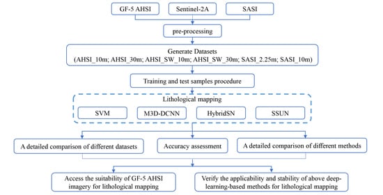
3.3. Methods and Experimental Design

3.3.1. Methods

From the perspective of deep learning, the components of HSI imagery are hierarchical. Specifically, pixels are first assembled to form edges, edges are then assembled to form parts, then parts are finally assembled to form different objects [55]. Therefore, the deep-learning-based methods show promise for hierarchically learning the deep features contained in HSI imagery. To verify the applicability and stability of deep learning-based methods in lithological mapping based on GF-5 AHSI imagery, a multi-scale 3D deep convolutional neural network (M3D-DCNN) [38], a hybrid spectral CNN (HybridSN) [40], a spectral–spatial unified network (SSUN) [34], and Support Vector Machine (SVM) [25] were adopted in this study. A brief overview of the above methods is provided below.
(1)
A multi-scale 3D deep convolutional neural network (M3D-DCNN) [38] was proposed for HSI classification, which could jointly learn both 2D multi-scale spatial features [56] and 1D spectral features from HSI data in an end-to-end approach. A five-layer M3D-DCNN was finally applied for HSI classification. The smaller kernel size, deeper layers, and fewer parameters enable M3D-DCNN to mitigate the over-fitting problem in small HSI datasets. The source code can be found at https://github.com/eecn/Hyperspectral-Classification.
(2)
The hybrid spectral CNN (HybridSN) [40] is a spectral–spatial 3D-CNN followed by spatial 2D-CNN. The 3D-CNN [57] facilitates the joint spectral–spatial feature representation from a stack of spectral bands, and the 2D-CNN on top of the 3D-CNN further learns more abstract-level spatial representation. The 3D- and 2D-CNN layers are assembled so that they can use both the spectral and spatial feature maps to their full extent to achieve the maximum possible accuracy. HybridSN is more computationally efficient than the 3D-CNN model [58]. The source code can be found at https://github.com/gokriznastic/HybridSN.
(3)
The spectral–spatial unified network (SSUN) [34] combines spectral and spatial feature extraction as well as classifier training in a unified network, which means both feature extraction and classifier training share a uniform objective function and all the parameters in the network can be optimized simultaneously. In other words, the learned features become more discriminative since the loss function of the network considers both spectral and spatial information. In the implementation of the SSUN, spatial information is learned by a multiscale convolutional neural network (MSCNN), and the extraction of spectral feature is by means of a band grouping-based long short-term memory (LSTM) algorithm [59]. In this experiment, the grouping strategy 2 was adopted, which focuses on the global features on the spectral dimension [60]. The source code can be found at https://github.com/YonghaoXu/SSUN.
(4)
As a typical representative of machine-learning-based methods, the SVM algorithm was selected for comparative analysis with deep-learning-based techniques to verify the advantages of deep-learning-based methods. SVM [25,61] has often been found to provide higher classification accuracy than other widely used machine-learning-based techniques, such as the maximum likelihood and neural net classifiers. SVM does not require an estimation of the statistical distributions of classes but defines the classification model by exploiting the concept of margin maximization with an optimal separation hyperplane. SVM has excellent performance in hyperspectral remote sensing classification due to the description of the complexity, which can be characterized by the number of support vectors rather than the dimensions of the transformation space [62]. In this study, lithological mapping by SVM was implemented in ENVI5.3 software (Harris Geospatial Solutions, Inc., Broomfield, CO, USA), and radial basis function (RBF) was chosen as the kernel function [63].

3.3.2. Experimental Design

In our experiments, six hyperspectral datasets constructed from GF-5 AHSI imagery, the fused hyperspectral imagery, and SASI imagery were used. Diverse datasets were used to comprehensively test the applicability of GF-5 AHSI data, and various methods were used to find a more suitable deep learning framework for lithological mapping. The details of the six datasets are provided in Table 5. Before the samples procedure, the normalized difference vegetation index (NDVI) was calculated based on S2A imagery. And the mean of NDVI was about 0.11, which indicated that the vegetation coverage in the area was low and the bedrock was well exposed. Therefore, vegetation interference would not be considered in the follow-up study. Since the datasets have three different spatial resolutions (10, 30, and 2.25 m, respectively), when selecting samples, the area covered by the samples of all datasets must be equal, which means that the samples occupy the same proportion in the whole image. The labels of the samples are determined by the geological map (Figure 1) and are numbered from young to old by age. The samples should be distributed evenly throughout the whole study area and avoid the boundaries of different litho-units. The sample size of each category is shown in Table 6, and the sample distribution is shown in Figure 4.
After repeated attempts, the model settings were determined as shown in Table 7. Since the framework of each model is different, it was difficult to keep all the parameters consistent. To facilitate comparison of the results produced by the above methods, the same parameter settings were adopted as much as possible under the premise of adhering to the structure of the model and following the original authors’ parameter setting recommendations. In all the experiments, 30% of all samples were selected as training samples and the rest as test samples. And Principal Component Analysis (PCA) was used for dimension reduction of HybridSN and SSUN. For some other parameters not mentioned in Table 7, such as the number of convolutional layers, kernel number, kernel size, kernel stride, batch size, number of epochs, etc., the defaults were used (Supplementary Table S1–S8). In addition, classification maps classified by SVM would be post-classification processed using majority analysis, and its kernel size is shown in Table 7.
As shown in Table 7, since the HybridSN model needs to use 3D-CNN to complete spectral–spatial feature learning, more principal component bands need to be retained. Compared with HybridSN, the spatial information of SSUN is extracted by MSCNN, while the spectral feature is learned by a band grouping-based LSTM algorithm, so it is sufficient to keep the first four principal component bands for learning spatial features. In addition, M3D-DCNN does not require any pre-processing. The window sizes of HybridSN and SSUN are consistent, whereas M3D-DCNN is relatively small due to the design of the smaller kernel size.
Finally, we used the overall accuracy (OA), user’s accuracy (UA), producer’s accuracy (PA), and kappa coefficient (Kappa) evaluation measures to judge the lithological mapping performance.

4. Results

The results are shown in Figure 5, which contains the lithological classification maps of SVM, M3D-DCNN, HybridSN, and SSUN methods, but does not include the intermediate results of SSUN (LSTM and MSCNN).
The Kappa and OA of the classification results, including those of LSTM and MSCNN, are shown in Table 8. The UA and PA for each dataset are represented as boxplots in Figure 6.

5. Discussion

In terms of the overall accuracy, all methods produced encouraging lithological mapping results on all datasets (OA > 90%). However, according to the lithological classification maps (Figure 5) and the boxplots (Figure 6), the classification results of Class 4 and 12 are relatively unstable and low accuracy. Class 4 is hornstone and slate, which are confused with Class 6 (slate) and Class 10 (slate and phyllite) due to their similarity in material composition. The area covered by Class 4 is low-lying, which easily accumulates other materials transported from the mountainous or surrounding areas. Class 12 (indosinian biotite granite) is confused with class 11 (indosinian granite), and the misclassified areas are mainly affected by mining activities.
From the perspective of datasets (Figure 7a), the classification accuracies of SASI_2.25 m and AHSI_10 m datasets were the highest and most stable, whereas the accuracy of AHSI_30 m was relatively low, but the stability was good. The classification results based on the short-wave infrared (SWIR) wavelength subset of GF-5 AHSI data differed little from SASI data in accuracy and were basically equal to those based on the full AHSI wavelength, indicating that AHSI’s SW bands have high SNR, which can basically meet the needs of geological mapping.
Due to the complex nature of geological processes resulting in the diversity of surface lithologies, classification accuracy could only explain a part of the results, the actual classification maps are also very important. It can be seen from Figure 5 that in the southeast corner of the study area, some classification maps have Class 3 (basalt with slate) divided into Class 2 (hornstone and sandstone) by mistake. The misclassified areas mainly correspond to the shadow of the mountain, and the datasets generated by AHSI imagery are more sensitive to it. Besides, the results of the eastern area (Figure 5) differ somewhat from the geological map (Figure 8a). There are two points to note here. First, due to the geological map itself is the product of artificial processing and synthesis of the real earth surface, there are different degrees of processing under different scales. In the process of geological map making, many lithological contact boundaries are obtained by reasoning, while remote sensing images are the real reflection of the surface, so the geological map lacks the verifiability of surface pixel by pixel [64]. Furthermore, because of the excessively trivial and complex surface conditions (Figure 8b), simplified processing was carried out in the 1:50,000 original geological map and the lithologies of this part are uncertain. We did not modify our geological map of this part according to the imagery, nor did we select samples in this area. Second, the lack of samples in this area leads to the fact that these differences are not included in the accuracy calculation. To a certain extent, these differences reflect the real condition of the surface, which is more consistent with the remote sensing imagery.
As for the methods (Figure 7b), SVM performed well in each dataset, and the deep-learning-based methods were slightly better than SVM. Because of the smaller kernel, M3D-DCNN is relatively stable and showed more accurate classification results on various datasets, demonstrating its higher robustness. In litho-units with small distribution area, over-smoothing always occurs during the execution of HybridSN, especially in datasets with low spatial resolution. In paper [40], HybridSN showed advantages over M3D-DCNN in Indian Pines, University of Pavia, and Salinas Scene datasets, containing classes with consistent scales and regular texture features, which are essentially different from the litho-units. LSTM produced a good classification effect and takes full advantage of the rich spectral information of HSI. However, the feature extraction of MSCNN is relatively unstable, which is related to the texture similarity of adjacent lithological units caused by surface weathering and transportation. Therefore, although the average accuracy of SSUN was the highest, we observed some differences in the classification effects on different datasets. The SSUN method is more effective on datasets with high spatial resolution.

6. Conclusions

We increased the spatial resolution of the fused AHSI imagery from 30 to 10 m, with high classification accuracy and stable application in various methods. The original AHSI imagery also produced encouraging classification results. And it also can produce comparable results by just only using the short-wave infrared wavelength subset (SWIR bands) of GF-5 AHSI data, which means AHSI SWIR bands contain most of the surface lithological information and could meet the needs of geological mapping. By comparison with the SASI data, we found that the classification accuracies obtained by AHSI SWIR bands are lower than that of SASI data, but the difference is not significant, which verifies the AHSI SWIR bands have a high SNR. Therefore, GF-5 AHSI data shows promise to provide more suitable data for lithological mapping.
Generally, the classification effect of deep-learning-based methods is better than machine-learning-based methods. M3D-DCNN has high classification accuracy and a stable classification effect, whereas HybridSN is prone to over-smoothing. Although the SSUN method has higher average accuracy, the classification effect is relatively unstable when dealing with lithological mapping with irregular boundaries, inconsistent scales, and similar textures in adjacent units, so it is more suitable for datasets with higher spatial resolution.
To sum up, GF-5 AHSI data can meet the needs of large-area and large-scale lithological mapping. Especially, it can produce comparable results by just only using the short-wave infrared wavelength subset (SWIR bands) of GF-5 AHSI data. Therefore, GF-5 AHSI imagery is recommended when performing large-area and large-scale lithological mapping. and M3D-DCNN method is also recommended for use in lithological mapping based on hyperspectral data. The extraction of irregular surface texture information and the determination of convolution kernel size will be the focus of subsequent research.

Supplementary Materials

The following are available online at https://0-www-mdpi-com.brum.beds.ac.uk/2072-4292/12/23/3990/s1, Table S1: Parameters of convolutional layers in M3D-DCNN method. Table S2: Other parameters of M3D-DCNN method. Table S3: Parameters of layers in HybridSN method. Table S4: Other parameters of HybridSN method. Table S5: Parameters of LSTM layers in SSUN method. Table S6: Parameters of MSCNN layers in SSUN method. Table S7: Other parameters of SSUN method. Table S8: Parameters of SVM-RBF method.

Author Contributions

Conceptualization, B.Y. and S.T.; methodology, B.Y.; software, Y.G.; validation, B.Y., Y.G., and Q.C.; formal analysis, B.Y. and Q.C.; investigation, B.Y.; resources, S.T.; data curation, S.T.; writing—original draft preparation, B.Y.; writing—review and editing, B.Y. and Y.G.; visualization, Y.G.; supervision, Q.C.; project administration, S.T.; funding acquisition, S.T. All authors have read and agreed to the published version of the manuscript.

Funding

This research was funded by Comprehensive Investigation and Evaluation on the Carrying Capacity of Resources and Environment, Grant Number DD20190301.

Acknowledgments

Regional geological maps and geological background material were provided by China Aero Geophysical Survey and Remote Sensing Center (AGRS); GF-5 AHSI imagery was obtained from Land Satellite Remote Sensing Application Center of Ministry of Natural Resources, China; and SASI data were provided by Beijing Research Institute of Uranium Geology. We express our sincere thanks. We are also grateful to the European Space Agency (ESA) Copernicus Open Access Hub (https://scihub.copernicus.eu/) for providing Sentinel-2 data. Thanks also go to editors and the anonymous reviewers for helping us to improve the quality of the manuscript.

Conflicts of Interest

The authors declare no conflict of interest.

References

  1. Pal, M.; Rasmussen, T.; Porwal, A. Optimized lithological mapping from multispectral and hyperspectral remote sensing images using fused multi-classifiers. Remote Sens. 2020, 12, 177. [Google Scholar] [CrossRef] [Green Version]
  2. Bioucas-Dias, J.M.; Plaza, A.; Dobigeon, N.; Parente, M.; Du, Q.; Gader, P.; Chanussot, J. Hyperspectral Unmixing Overview: Geometrical, Statistical, and Sparse Regression-Based Approaches. IEEE J. Sel. Top. Appl. Earth Obs. Remote Sens. 2012, 5, 354–379. [Google Scholar] [CrossRef] [Green Version]
  3. Kruse, F.A.; Boardman, J.W.; Huntington, J.F. Comparison of airborne hyperspectral data and EO-1 Hyperion for mineral mapping. IEEE Trans. Geosci. Remote Sens. 2003, 41, 1388–1400. [Google Scholar] [CrossRef] [Green Version]
  4. Bing-xiang, T.; Li, Z.; Chen, E.; Pang, Y. Preprocessing of EO-1 Hyperion Hyperspectral Data. Remote Sens. Inf. 2005, 6, 36–41. [Google Scholar]
  5. Earth Observing One EO-1—Hyperion. Available online: https://www.usgs.gov/centers/eros/science/usgs-eros-archive-earth-observing-one-eo-1-hyperion?qt-science_center_objects=0#qt-science_center_objects (accessed on 18 November 2020).
  6. Kumar, H.; Rajawat, A.S. Aqueous alteration mapping in Rishabdev ultramafic complex using imaging spectroscopy. Int. J. Appl. Earth Obs. Geoinf. 2020, 88, 102084. [Google Scholar] [CrossRef]
  7. Tripathi, M.K.; Govil, H. Evaluation of AVIRIS-NG hyperspectral images for mineral identification and mapping. Heliyon 2019, 5, e02931. [Google Scholar] [CrossRef]
  8. Bedini, E. Mineral mapping in the Kap Simpson complex, central East Greenland, using HyMap and ASTER remote sensing data. Adv. Space Res. 2011, 47, 60–73. [Google Scholar] [CrossRef]
  9. Graham, G.E.; Kokaly, R.F.; Kelley, K.D.; Hoefen, T.M.; Johnson, M.R.; Hubbard, B.E. Application of Imaging Spectroscopy for Mineral Exploration in Alaska: A Study over Porphyry Cu Deposits in the Eastern Alaska Range. Econ. Geol. 2018, 113, 489–510. [Google Scholar] [CrossRef]
  10. Jing, C.; Bokun, Y.; Runsheng, W.; Feng, T.; Yingjun, Z.; Dechang, L.; Suming, Y.; Wei, S. Regional-scale mineral mapping using ASTER VNIR/SWIR data and validation of reflectance and mineral map products using airborne hyperspectral CASI/SASI data. Int. J. Appl. Earth Obs. Geoinf. 2014, 33, 127–141. [Google Scholar] [CrossRef]
  11. Manzo, C.; Valentini, E.; Taramelli, A.; Filipponi, F.; Disperati, L. Spectral characterization of coastal sediments using Field Spectral Libraries, Airborne Hyperspectral Images and Topographic LiDAR Data (FHyL). Int. J. Appl. Earth Obs. Geoinf. 2015, 36, 54–68. [Google Scholar] [CrossRef]
  12. Forzieri, G.; Moser, G.; Catani, F. Assessment of hyperspectral MIVIS sensor capability for heterogeneous landscape classification. Isprs J. Photogramm. Remote Sens. 2012, 74, 175–184. [Google Scholar] [CrossRef]
  13. Liu, Y.; Sun, D.; Hu, X.; Liu, S.; Cao, K.; Chai, M.; Liao, Q.; Zuo, Z.; Hao, Z.; Duan, W.; et al. Development of Visible and Short-wave Infrared Hyperspectral Imager onboard GaoFen-5 Satellite. J. Remote Sens. (Chin.) 2020, 24, 333–344. [Google Scholar]
  14. GaoFen 5. Available online: https://nssdc.gsfc.nasa.gov/nmc/spacecraft/display.action?id=2018-043A (accessed on 18 November 2020).
  15. van der Meer, F.D.; van der Werff, H.M.A.; van Ruitenbeek, F.J.A.; Hecker, C.A.; Bakker, W.H.; Noomen, M.F.; van der Meijde, M.; Carranza, E.J.M.; de Smeth, J.B.; Woldai, T. Multi- and hyperspectral geologic remote sensing: A review. Int. J. Appl. Earth Obs. Geoinf. 2012, 14, 112–128. [Google Scholar] [CrossRef]
  16. Zhang, X.; Li, P. Lithological mapping from hyperspectral data by improved use of spectral angle mapper. Int. J. Appl. Earth Obs. Geoinf. 2014, 31, 95–109. [Google Scholar] [CrossRef]
  17. Hecker, C.; van der Meijde, M.; van der Werff, H.; van der Meer, F.D. Assessing the Influence of Reference Spectra on Synthetic SAM Classification Results. IEEE Trans. Geosci. Remote Sens. 2008, 46, 4162–4172. [Google Scholar] [CrossRef]
  18. vanderMeer, F.; Bakker, W. Cross correlogram spectral matching: Application to surface mineralogical mapping by using AVIRIS data from Cuprite, Nevada. Remote Sens. Environ. 1997, 61, 371–382. [Google Scholar] [CrossRef]
  19. Chang, C.I. An information-theoretic approach to spectral variability, similarity, and discrimination for hyperspectral image analysis. IEEE Trans. Inf. Theory 2000, 46, 1927–1932. [Google Scholar] [CrossRef] [Green Version]
  20. Xu, N.; Hu, Y.X.; Lei, B.; Hong, Y.T.; Dang, F.X. Mineral Information Extraction for Hyperspectral Image Based on Modified Spectral Feature Fitting Algorithm. Spectrosc. Spectr. Anal. 2011, 31, 1639–1643. [Google Scholar] [CrossRef]
  21. Laukamp, C.; Cudahy, T.; Thomas, M.; Jones, M.; Cleverley, J.S.; Oliver, N.H.S. Hydrothermal mineral alteration patterns in the Mount Isa Inlier revealed by airborne hyperspectral data. Aust. J. Earth Sci. 2011, 58, 917–936. [Google Scholar] [CrossRef]
  22. Cudahy, T.; Jones, M.; Thomas, M.; Laukamp, C.; Caccetta, M.; Hewson, R.; Rodger, A.; Verrall, M. Next Generation Mineral Mapping: Queensland Airborne HyMap and Satellite ASTER Surveys 2006–2008. In CSIRO Exploration and Mining Report, P2007/364; CSIRO: Canberra, Australia, 2008. [Google Scholar] [CrossRef]
  23. Jain, R.; Sharma, R.U. Airborne hyperspectral data for mineral mapping in Southeastern Rajasthan, India. Int. J. Appl. Earth Obs. Geoinf. 2019, 81, 137–145. [Google Scholar] [CrossRef]
  24. Fauvel, M.; Benediktsson, J.A.; Chanussot, J.; Sveinsson, J.R. Spectral and Spatial Classification of Hyperspectral Data Using SVMs and Morphological Profiles. IEEE Trans. Geosci. Remote Sens. 2008, 46, 3804–3814. [Google Scholar] [CrossRef] [Green Version]
  25. Melgani, F.; Bruzzone, L. Classification of hyperspectral remote sensing images with support vector machines. IEEE Trans. Geosci. Remote Sens. 2004, 42, 1778–1790. [Google Scholar] [CrossRef] [Green Version]
  26. Ham, J.; Chen, Y.C.; Crawford, M.M.; Ghosh, J. Investigation of the random forest framework for classification of hyperspectral data. IEEE Trans. Geosci. Remote Sens. 2005, 43, 492–501. [Google Scholar] [CrossRef] [Green Version]
  27. Belgiu, M.; Dragut, L. Random forest in remote sensing: A review of applications and future directions. ISPRS J. Photogramm. Remote Sens. 2016, 114, 24–31. [Google Scholar] [CrossRef]
  28. Lu, T.; Li, S.T.; Fang, L.Y.; Jia, X.P.; Benediktsson, J.A. From subpixel to superpixel: A novel fusion framework for hyperspectral image classification. IEEE Trans. Geosci. Remote Sens. 2017, 55, 4398–4411. [Google Scholar] [CrossRef]
  29. Han, T.; Goodenough, D.G. Investigation of nonlinearity in hyperspectral imagery using surrogate data methods. IEEE Trans. Geosci. Remote Sens. 2008, 46, 2840–2847. [Google Scholar] [CrossRef]
  30. Chen, Y.S.; Lin, Z.H.; Zhao, X.; Wang, G.; Gu, Y.F. Deep learning-based classification of hyperspectral data. IEEE J. Sel. Top. Appl. Earth Obs. Remote Sens. 2014, 7, 2094–2107. [Google Scholar] [CrossRef]
  31. Chen, Y.S.; Zhao, X.; Jia, X.P. Spectral-spatial classification of hyperspectral data based on deep belief network. IEEE J. Sel. Top. Appl. Earth Obs. Remote Sens. 2015, 8, 2381–2392. [Google Scholar] [CrossRef]
  32. Chen, Y.S.; Jiang, H.L.; Li, C.Y.; Jia, X.P.; Ghamisi, P. Deep feature extraction and classification of hyperspectral images based on convolutional neural networks. IEEE Trans. Geosci. Remote Sens. 2016, 54, 6232–6251. [Google Scholar] [CrossRef] [Green Version]
  33. Yu, S.Q.; Jia, D.; Xu, C.Y. Convolutional neural networks for hyperspectral image classification. Neurocomputing 2017, 219, 88–98. [Google Scholar] [CrossRef]
  34. Xu, Y.H.; Zhang, L.P.; Du, B.; Zhang, F. Spectral-spatial unified networks for hyperspectral image classification. IEEE Trans. Geosci. Remote Sens. 2018, 56, 5893–5909. [Google Scholar] [CrossRef]
  35. Chen, J.X.; Pisonero, J.; Chen, S.; Wang, X.; Fan, Q.W.; Duan, Y.X. Convolutional neural network as a novel classification approach for laser-induced breakdown spectroscopy applications in lithological recognition. Spectroc. Acta Part B At. Spectr. 2020, 166, 7. [Google Scholar] [CrossRef]
  36. Anjos, C.E.M.D.; Avila, M.R.V.; Vasconcelos, A.G.P.; Neta, A.M.P.; Surmas, R. Deep learning for lithological classification of carbonate rock micro-CT images. arXiv 2020, arXiv:2007.15693. [Google Scholar]
  37. Brandmeier, M.; Chen, Y. Lithological classification using multi-sensor data and convolutional neural networks. Isprs. Int. Arch. Photogramm. Remote Sens. Spat. Inf. Sci. 2019, XLII-2/W16, 55–59. [Google Scholar] [CrossRef] [Green Version]
  38. He, M.Y.; Li, B.; Chen, H.H. Multi-Scale 3d Deep Convolutional Neural Network for Hyperspectral Image Classification. In Proceedings of the 2017 24th Ieee International Conference on Image Processing, Beijing, China, 17–20 September 2017; IEEE: New York, NY, USA, 2017; pp. 3904–3908. [Google Scholar] [CrossRef]
  39. Zhao, W.Z.; Du, S.H. Spectral-Spatial Feature Extraction for Hyperspectral Image Classification: A Dimension Reduction and Deep Learning Approach. IEEE Trans. Geosci. Remote Sens. 2016, 54, 4544–4554. [Google Scholar] [CrossRef]
  40. Roy, S.K.; Krishna, G.; Dubey, S.R.; Chaudhuri, B.B. HybridSN: Exploring 3-D-2-D CNN Feature Hierarchy for Hyperspectral Image Classification. IEEE Geosci. Remote Sens. Lett. 2020, 17, 277–281. [Google Scholar] [CrossRef] [Green Version]
  41. Jiyuan, Y.; Guoqiang, W.; Xiangmin, L.; Bo, J.; Qiaojuan, Y. The redefinition of huaniushan group in beishan area: Geochemical evidence from volcanic rocks. Xinjiang Geol. 2015, 33, 537–543. [Google Scholar]
  42. Che, Y.; Zhao, Y. CASI/SASI Airborne Hyperspectral Remote Sensing Anomaly Extraction of Metallogenic Prediction Research in Gansu Beishan South Beach area. In Proceedings of the Conference on Multispectral, Hyperspectral, and Ultraspectral Remote Sensing Technology, Techniques and Applications V, Beijing, China, 18 November 2014; SPIE: Bellingham, WA, USA, 2014; Volume 9263. [Google Scholar] [CrossRef]
  43. Liu, Y.N.; Sun, D.X.; Hu, X.N.; Ye, X.; Li, Y.D.; Liu, S.F.; Cao, K.Q.; Chai, M.Y.; Zhou, W.Y.N.; Zhang, J.; et al. The Advanced Hyperspectral Imager Aboard China’s GaoFen-5 satellite. IEEE Geosci. Remote Sens. Mag. 2019, 7, 23–32. [Google Scholar] [CrossRef]
  44. Corner, B.R.; Narayanan, R.M.; Reichenbach, S.E. Noise estimation in remote sensing imagery using data masking. Int. J. Remote Sens. 2003, 24, 689–702. [Google Scholar] [CrossRef]
  45. Liu, Y.; Sun, D.; Cao, K.; Liu, S.; Chai, M.; Liang, J.; Yuan, J. Evaluation of GaoFen-5/AHSI on-orbit instrument radiometric performance. J. Remote Sens. (Chin.) 2019, 16, 7–22. [Google Scholar]
  46. Spoto, F.; Sy, O.; Laberinti, P.; Martimort, P.; Fernandez, V.; Colin, O.; Hoersch, B.; Meygret, A. Overview of Sentinel-2. In Proceedings of the 2012 IEEE International Geoscience and Remote Sensing Symposium, Munich, Germany, 22–27 July 2012; IEEE: Piscataway, NJ, USA, 2012; pp. 1707–1710. [Google Scholar]
  47. Sentinel 2. Available online: https://blogs.fu-berlin.de/reseda/sentinel-2/ (accessed on 18 November 2020).
  48. Drusch, M.; Del Bello, U.; Carlier, S.; Colin, O.; Fernandez, V.; Gascon, F.; Hoersch, B.; Isola, C.; Laberinti, P.; Martimort, P.; et al. Sentinel-2: ESA’s Optical high-resolution mission for GMES operational services. Remote Sens. Environ. 2012, 120, 25–36. [Google Scholar] [CrossRef]
  49. ESA Copernicus Open Access Hub. Available online: https://scihub.copernicus.eu/ (accessed on 18 November 2020).
  50. Wang, J.J.; Zhang, Y.; Bussink, C. Unsupervised multiple endmember spectral mixture analysis-based detection of opium poppy fields from an EO-1 hyperion image in Helmand, Afghanistan. Sci. Total Env. 2014, 476, 1–6. [Google Scholar] [CrossRef] [PubMed]
  51. Cooley, T.; Anderson, G.P.; Felde, G.W.; Hoke, M.L.; Ratkowski, A.J.; Chetwynd, J.H.; Gardner, J.A.; Adler-Golden, S.M.; Matthew, M.W.; Berk, A.; et al. FLAASH, a MODTRAN4-based atmospheric correction algorithm, its application and validation. In Proceedings of the Igarss 2002: IEEE International Geoscience and Remote Sensing Symposium and 24th Canadian Symposium on Remote Sensing, Vols I-Vi, Proceedings: Remote Sensing: Integrating Our View of the Planet, Toronto, ON, Canada, 24–28 June 2002; IEEE: New York, NY, USA, 2002; pp. 1414–1418. [Google Scholar]
  52. Green, A.A.; Berman, M.; Switzer, P.; Craig, M.D. A transformation for ordering multispectral data in terms of image quality with implications for noise removal. IEEE Trans. Geosci. Remote Sens. 1988, 26, 65–74. [Google Scholar] [CrossRef] [Green Version]
  53. Zizala, D.; Zadorova, T.; Kapicka, J. Assessment of soil degradation by erosion based on analysis of soil properties using aerial hyperspectral images and ancillary data, Czech Republic. Remote Sens. 2017, 9, 28. [Google Scholar] [CrossRef] [Green Version]
  54. Main-Knorn, M.; Pflug, B.; Louis, J.; Debaecker, V.; Muller-Wilm, U.; Gascon, F. Sen2Cor for Sentinel-2. In Image and Signal Processing for Remote Sensing Xxiii; Bruzzone, L., Bovolo, F., Eds.; Spie-Int Soc Optical Engineering: Bellingham, WA, USA, 2017; Volume 10427. [Google Scholar]
  55. Hinton, G.E.; Salakhutdinov, R.R. Reducing the dimensionality of data with neural networks. Science 2006, 313, 504–507. [Google Scholar] [CrossRef] [Green Version]
  56. Srivastava, N.; Hinton, G.; Krizhevsky, A.; Sutskever, I.; Salakhutdinov, R. Dropout: A simple way to prevent neural networks from overfitting. J. Mach. Learn. Res. 2014, 15, 1929–1958. [Google Scholar]
  57. Ji, S.W.; Xu, W.; Yang, M.; Yu, K. 3D convolutional neural networks for human action recognition. IEEE Trans. Pattern Anal. Mach. Intell. 2013, 35, 221–231. [Google Scholar] [CrossRef] [Green Version]
  58. Roy, S.K.; Chatterjee, S.; Bhattacharyya, S.; Chaudhuri, B.B.; Platos, J. Lightweight spectral-spatial squeeze-and-excitation residual bag-of-features learning for hyperspectral classification. IEEE Trans. Geosci. Remote Sens. 2020, 58, 5277–5290. [Google Scholar] [CrossRef]
  59. Hochreiter, S.; Schmidhuber, J. Long short-term memory. Neural Comput. 1997, 9, 1735–1780. [Google Scholar] [CrossRef]
  60. Xu, Y.H.; Du, B.; Zhang, L.P.; Zhang, F. A Band Grouping Based LSTM Algorithm for Hyperspectral Image Classification. In Computer Vision, Pt Ii; Yang, J., Hu, Q., Cheng, M.M., Wang, L., Liu, Q., Bai, X., Meng, D., Eds.; Springer-Verlag Singapore Pte Ltd.: Singapore, 2017; Volume 772, pp. 421–432. [Google Scholar]
  61. Mountrakis, G.; Im, J.; Ogole, C. Support vector machines in remote sensing: A review. Isprs. J. Photogramm. Remote Sens. 2011, 66, 247–259. [Google Scholar] [CrossRef]
  62. Ye, B.; Tian, S.F.; Ge, J.; Sun, Y.Q. Assessment of WorldView-3 Data for Lithological Mapping. Remote Sens. 2017, 9, 1132. [Google Scholar] [CrossRef]
  63. Kuo, B.C.; Ho, H.H.; Li, C.H.; Hung, C.C.; Taur, J.S. A kernel-based feature selection method for svm with rbf kernel for hyperspectral image classification. IEEE J. Sel. Top. Appl. Earth Obs. Remote Sens. 2014, 7, 317–326. [Google Scholar] [CrossRef]
  64. Yu, L.; Porwal, A.; Holden, E.J.; Dentith, M.C. Towards automatic lithological classification from remote sensing data using support vector machines. Comput. Geosci. 2012, 45, 229–239. [Google Scholar] [CrossRef]
Figure 1. Simplified provincial boundary map of China and the location of the study area. A geological map of the study area is shown on the left, which was derived from an initial geological map at 1:50,000. The geological map is not shown strictly in accordance with the criteria, but in other bright and easily distinguishable colors to more clearly show the spatial distribution and boundaries of litho-units.
Remotesensing 12 03990 g001
Figure 2. Signal-to-noise ratio (SNR) measurement results of GF-5 AHSI imagery (a) in VNIR bands and (b) in SWIR bands (modified after Liu et al. [45]). The gray spectral range indicates the bands to be removed during pre-processing, and the blue line refers to the position with a SNR of 200.
Remotesensing 12 03990 g002
Figure 3. Preprocessed images. (a) GF-5 AHSI imagery (R: Band 62; G: Band 36; B: Band 20); (b) the fused hyperspectral imagery (R: Band 62; G: Band 36; B: Band 20); (c) SASI imagery (R: Band 75; G: Band 30; B: Band 5).
Remotesensing 12 03990 g003
Figure 4. Sample distribution map. The numbers in Sentinel-2A imagery (R: Band 4; G: Band 3; B: Band 2) and on the left side of legend represent the class numbers.
Remotesensing 12 03990 g004
Figure 5. Lithological classification maps. From left to right are the results of SVM, M3D-DCNN, HybridSN, and SSUN. Each row of results was produced from the same dataset, and different rows represent different datasets. From top to bottom are the results of AHSI_10 m (ad), AHSI_30 m (eh), AHSI_SW_10 m (il), AHSI_SW_30 m (mp), SASI_2.25 m (qt), and SASI_10 m (ux) datasets.
Remotesensing 12 03990 g005aRemotesensing 12 03990 g005b
Figure 6. Boxplots of user’s accuracy and producer’s accuracy for each dataset: (a) AHSI_10 m; (b) AHSI_30 m; (c) AHSI_SW_10 m; (d) AHSI_SW_30 m; (e) SASI_2.25 m; (f) SASI_10 m.
Remotesensing 12 03990 g006
Figure 7. Boxplots of overall accuracy for every (a) dataset and (b) method.
Remotesensing 12 03990 g007
Figure 8. (a) Geological map of the eastern part of the study area; (b) Sentinel-2A imagery (R: Band 4; G: Band 3; B: Band 2) and the samples are shown. The area circled in yellow is where the classification results are partially different from the geological map. Refer to Figure 1 and Figure 4 for legend.
Remotesensing 12 03990 g008
Table 1. Gaofen-5 (GF-5) satellite specification and major orbit parameters.
Orbit ParametersParameter Settings
Orbital typeSun synchronous orbit
Nominal orbital altitude708.45 km
Dip angle98.218
Orbital flat period98.805 min
Eccentricity ratio<0.0001
Flight cylinder number every day14.57
Orbital intercept24.731
Local time of descending node13:30
SensorsAdvanced Hyperspectral Imager (AHSI)
Visual and Infrared Multispectral Sensor (VIMS)
Greenhouse Gases Monitoring Instrument (GMI)
Atmospheric Infrared Ultraspectral (AIUS)
Environment Monitoring Instrument (EMI)
Directional Polarization Camera (DPC)
Table 2. Comparison of Gaofen-5 (GF-5) Advanced Hyperspectral Imager (AHSI) and Hyperion data.
ParametersAdvanced Hyperspectral Imager (AHSI)Hyperion Sensor
Wavelength Range0.4–2.5 μm0.4–2.5 μm
Spatial Resolution30 m30 m
Swath Width60 km7.5 km
Spectral ResolutionVNIR: 5 nm; SWIR: 10 nm10 nm
Number of BandsVNIR: 150; SWIR: 180VNIR: 70; SWIR: 172
SWIR Signal-to-Noise Ratio (SNR)~500~50
Table 3. Technical indexes of the Shortwave Infrared Airborne Spectrographic Imager (SASI).
ParameterSASI-600ParameterSASI-600
Spectral Range (nm)950–2450SNR (Peak Value)>1100
Number of Continuous Spectral Channels100Absolute Radiometric Accuracy (%)<2
Total Field of View (degrees)40Spectral Resolution (nm)15
Instantaneous Field of View (degrees)0.070Spatial Resolution (m)2.25
Table 4. Main parameters of fast line-of-sight atmospheric analysis of spectral hypercubes (FLAASH) atmospheric correction.
Parameter ValueParameter Value
Scene Center LocationLat: 41.19; Lon: 95.58Water RetrievalYes
Sensor Altitude (km)705Water Absorption (nm)1135
Ground Elevation (km)1.821Aerosol ModelRural
Pixel Size (m)30Aerosol Retrieval2-Band (K-T)
Flight Date2019/10/10Initial Visibility (km)40.00
Flight Time GMT 06:32:21Spectral PolishingYes
Atmospheric ModelSub-Arctic SummerWidth (Number of Bands)9
Table 5. Detailed introduction of six datasets.
Dataset NameSource of the Dataset
AHSI_10 mGram–Schmidt Pan Sharpening of pre-processed S2A Band3 and GF-5 AHSI imagery, with a spatial resolution of 10 m
AHSI_30 mPre-processed GF-5 AHSI imagery, with a spatial resolution of 30 m
AHSI_SW_10 mSWIR data of the AHSI_10 m dataset
AHSI_SW_30 mSWIR data of AHSI_30 m dataset
SASI_2.25 mPre-processed SASI imagery, with a spatial resolution of 2.25 m
SASI_10 mObtained by bilinear resampling of pre-processed SASI imagery, with a spatial resolution of 10 m
Table 6. Sample size statistics.
Class LabelClass NameSample Area
(km2)
Map Area
(km2)
Percent
1Diluvial gravel and sand0.1471.391 10.57%
2Hornstone and sandstone0.1522.203 6.90%
3Basalt with slate0.5354.406 12.14%
4Hornstone and slate0.0971.447 6.70%
5Biotite felsic slate0.2092.275 9.19%
6Slate0.4393.106 14.13%
7Hornstone0.4154.553 9.11%
8Limestone0.1290.941 13.71%
9Marble with phyllite0.3052.194 13.90%
10Slate and phyllite0.3494.070 8.57%
11Indosinian granite0.4504.815 9.35%
12Indosinian biotite granite0.5705.192 10.98%
13Variscan diorite0.1200.715 16.78%
14Variscan granodiorite0.2021.768 11.43%
Sum4.11939.07610.54%
Table 7. Parameter settings of different models.
MethodParameterAHSI_
10 m
AHSI_
30 m
AHSI_SW_
10 m
AHSI_SW_
30 m
SASI_
10 m
SASI_
2.25 m
M3D-DCNNWindow Size777777
Hybrid
SN
PCA303030301515
Window Size191519151925
SSUNPCA444444
Window Size191519151925
SVM-RBFKernel size of post-classification757577
Table 8. Classification accuracy values for all experiments.
MethodsEvaluation MeasuresAHSI
_10 m
AHSI
_30 m
AHSI_SW
_10 m
AHSI_SW
_30 m
SASI
_2.25 m
SASI
_10 m
SVMKappa0.9620.9270.9250.8970.9800.954
OA96.48%93.28%93.13%90.55%98.19%95.81%
M3D-DCNNKappa0.9700.9470.9600.9740.9770.960
OA97.25%95.19%96.39%97.62%97.85%96.33%
HybridSNKappa0.9560.9470.9630.9480.9720.923
OA95.96%95.15%96.63%95.27%97.48%93.00%
LSTMKappa0.9670.9470.9660.9360.9960.959
OA96.96%95.15%96.91%94.14%99.60%96.78%
MSCNNKappa0.9390.9320.9390.9470.9850.996
OA94.42%93.78%94.44%95.15%98.78%99.69%
SSUNKappa0.9550.9730.9560.9660.9970.999
OA95.92%97.52%95.96%96.91%99.78%99.90%
Publisher’s Note: MDPI stays neutral with regard to jurisdictional claims in published maps and institutional affiliations.

