Analysis of the Possibilities of Using Different Resolution Digital Elevation Models in the Study of Microrelief on the Example of Terrain Passability


Abstract
:
1. Introduction
1.1. Related Works
1.2. Research Purpose
2. Test Area and Used Data
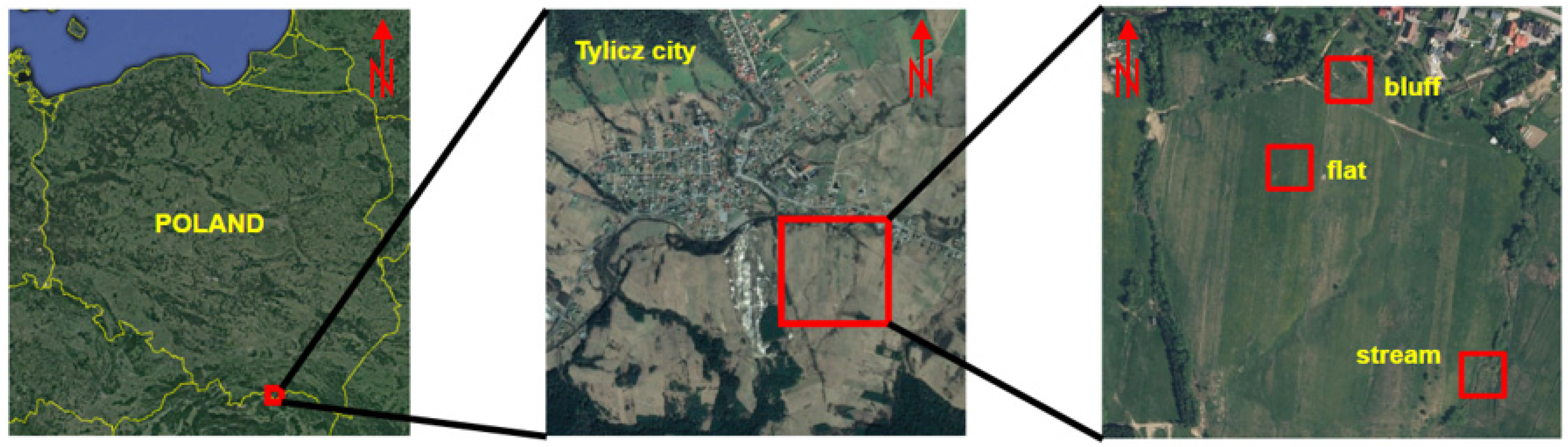
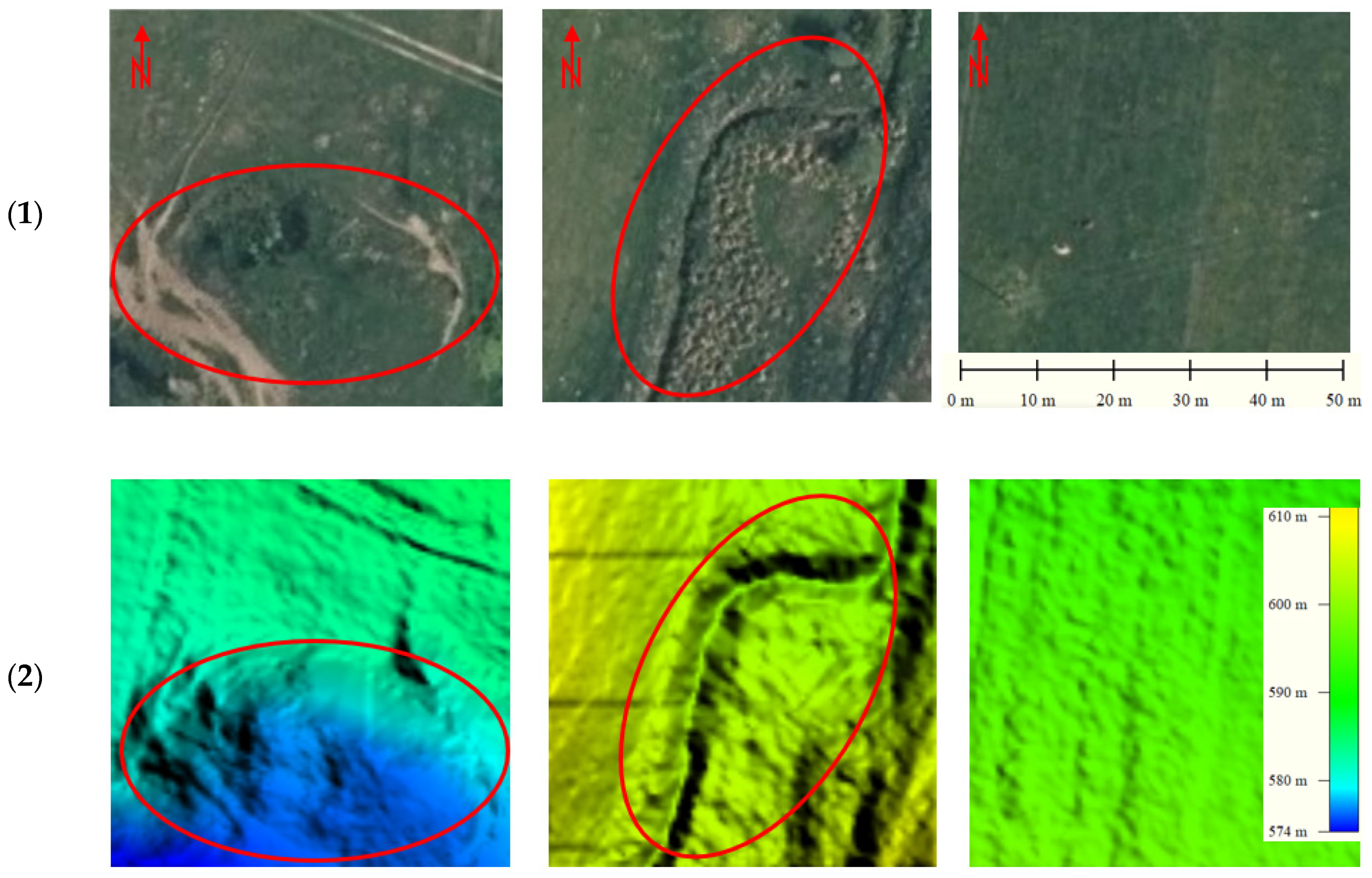
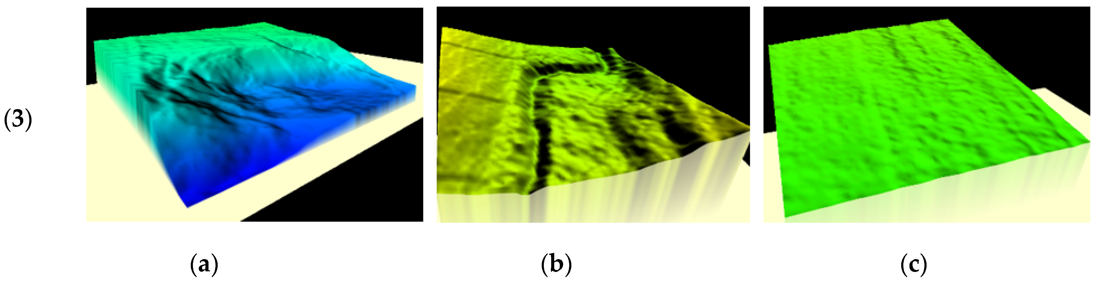
2.1. Area of Research
2.2. Geomatics Data Used in the Experimentation
3. Method
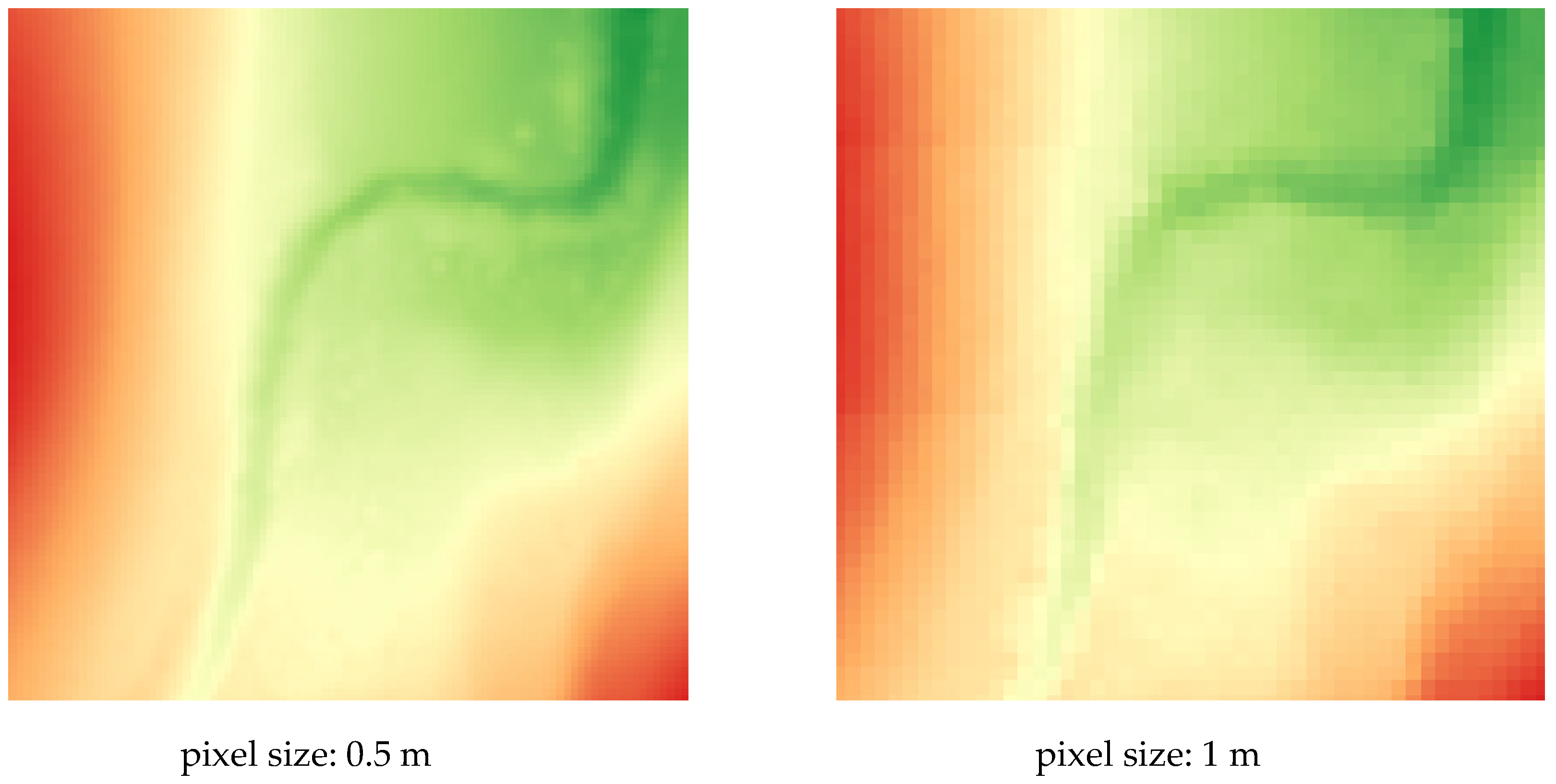
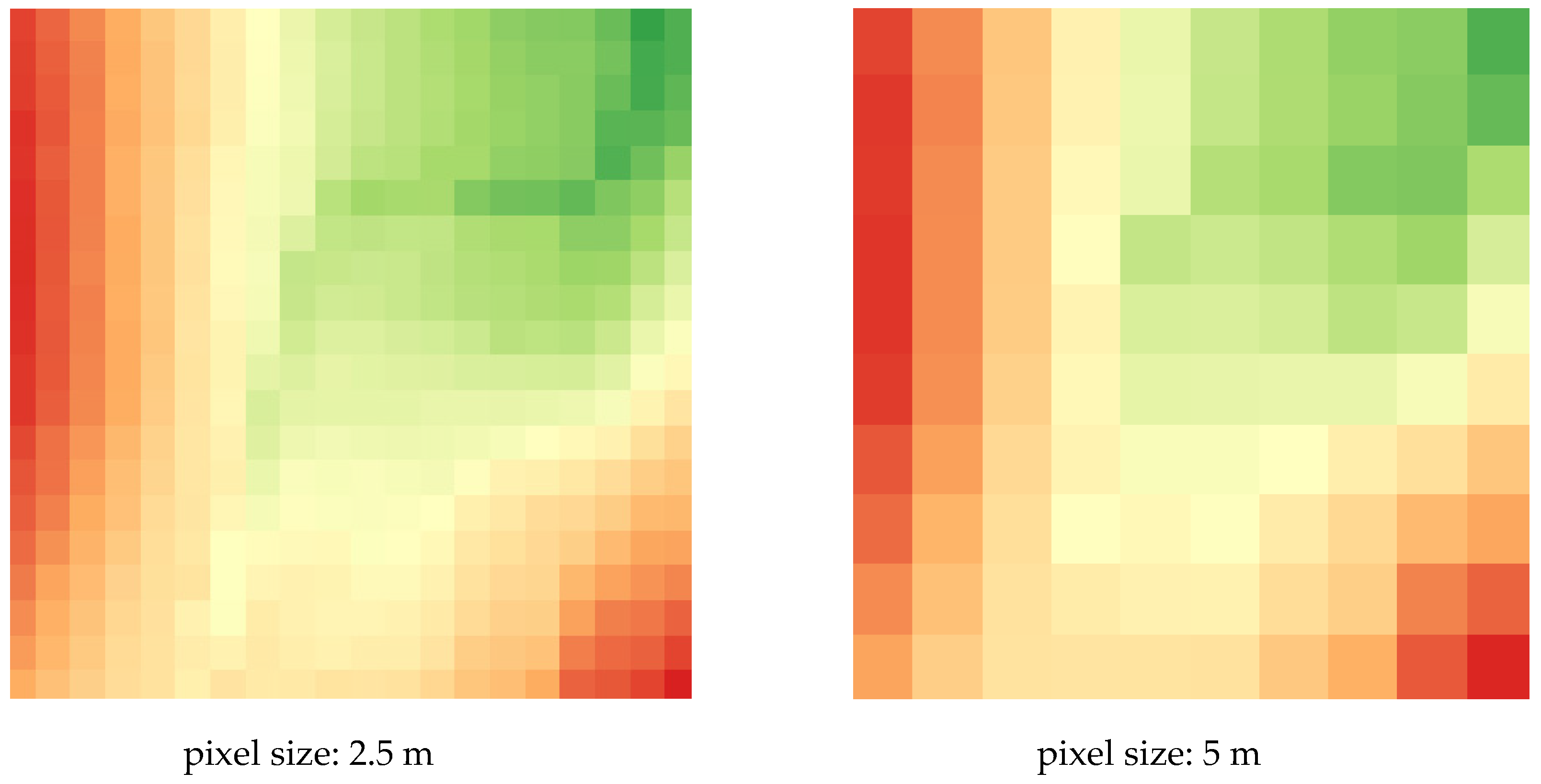
3.1. Preparing and Processing Data
- Binning—The determination of the pixel value relies on examining the points that fall within the defined pixel. The final value can be chosen as the minimum, maximum, or average of the points [51].
- Triangulation—To determine the final value, the Delaunay triangulation was used. This creates a surface made from a network of triangles and then rasterizes it.
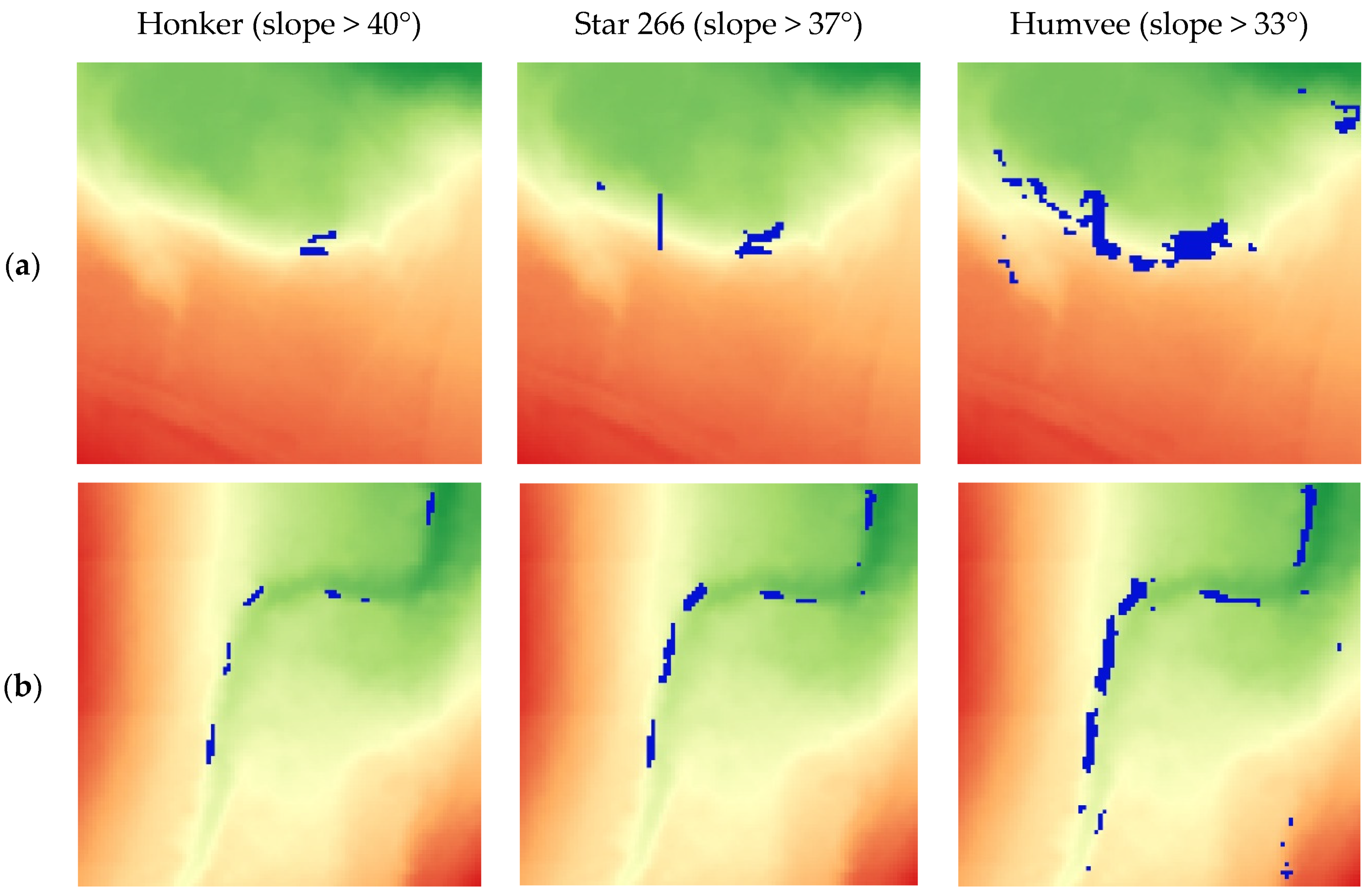
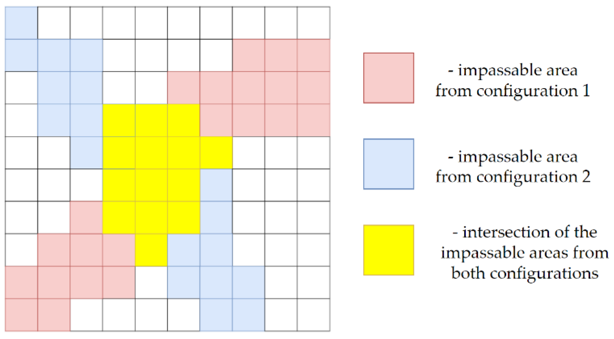
3.2. Terrain Passability Analysis Assumptions
3.3. The Principle of Working of the Developed Algorithm
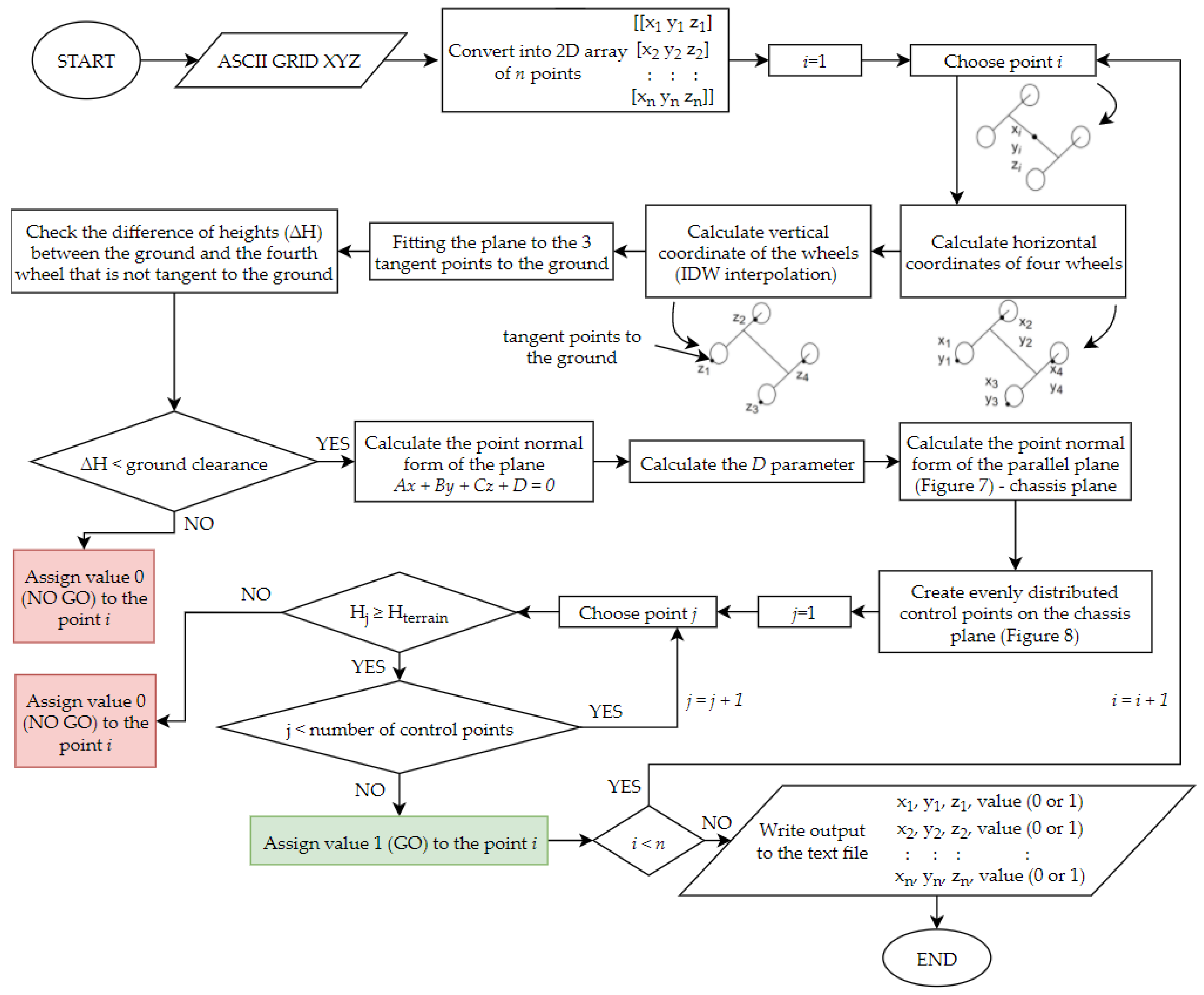
- The elevation model in ASCII XYZ Grid format is converted into a two-dimensional array with three columns (X, Y, Z) and a number of rows equal to the number of points in the model. The script is, thereby, able to perform the mathematical operations on the data.
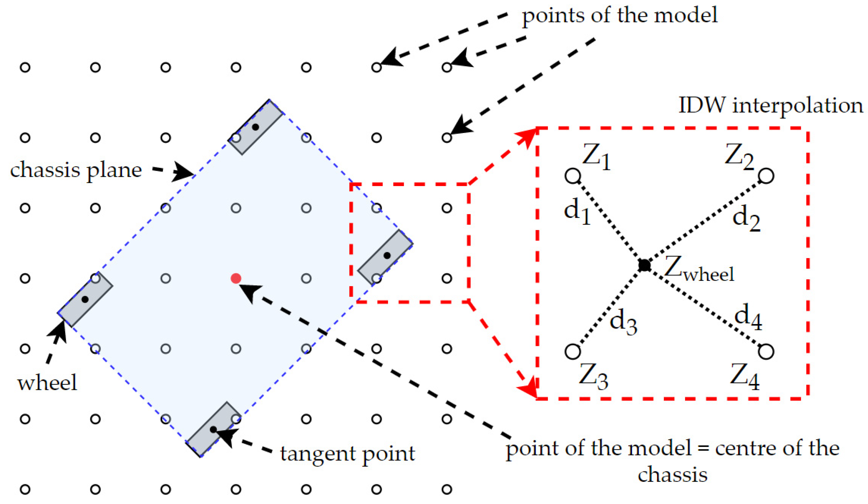
- The procedure from this point iterates through each point of the model (row in the array). The coordinates of selected points are assigned to the centroid of the chassis. On the basis of the wheelbase and track width there are calculated horizontal coordinates of the four wheels. The computation considers the local slope of the terrain because, when the vehicle is pitched, the horizontal dimensions must be reduced.
- Having calculated the coordinates of the wheels, the script computes the equation of the plane containing three tire contact points with the ground. At the beginning, four plane equations are calculated (containing three out of four tangent points in different configurations), and then the procedure searches in which plane position the fourth point of the vehicle (which does not belong to the plane) has the least difference of heights with the theoretical point with the same horizontal coordinates that belongs to the plane. After this test, the best fitted plane is chosen for further analysis. If the difference of heights is greater than the ground clearance, the analyzed point of the elevation model is assigned the value 0, which indicates that this point is impassable. The finding of the plane equation comes to the determination of four parameters of the point normal form of the plane (1):where A, B, C, and D are the parameters. The first three are calculated from the cross product of vectors created between two pairs of analyzed points, The D parameter is computed by the substitution of the coordinates of one analyzed point into formula (2).Ax + By + Cz + D = 0,where x, y, and z are the coordinates of one of the tangent points.D = −(Ax + By + Cz),
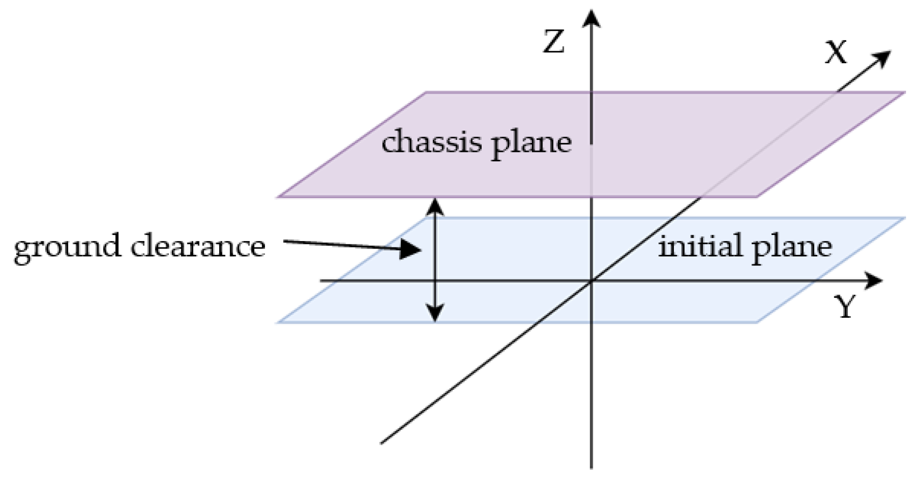
- The aim of the next step is to compute the plane that approximates the chassis plane. To do that, we must calculate the parallel plane to the one that has already been determined. The value of the shift (distance between two planes) is equal to the ground clearance. This situation is shown in Figure 8.
- This step extracts the part of the chassis plane that is limited by the wheels. Then, inside the resulting rectangle, the algorithm creates evenly distributed control points. It divides the distances between the wheels (wheelbase and track width) into even segments and places control points between them. As a result, we obtain a grid of points located in the chassis plane, which we can see in Figure 9. The distances between the points depend on the vehicle and especially on their parameters. The algorithm divides the wheelbase and track width values in each vehicle into four even parts.
- Finally, the script checks each control point for whether its height exceeds the height of the terrain interpolated from the model. Unless all points meet this requirement (are higher than points on terrain), the analyzed point of the model is assigned the value 0 (impassable).
- At the end of the process, the script creates a text file with coordinates of each point and an appended value of the passability (NO GO terrain—0 and GO terrain—1). On the basis of this file, we can distinguish the impassable terrain and calculate the statistics, which are presented further in the later section.
- Model: ASUS X556UAK
- Processor: Intel® Core™ i5-7200U CPU @ 2.71 GHz
- Operating system: Windows 10 ×64 operating system
- RAM: 20 GB
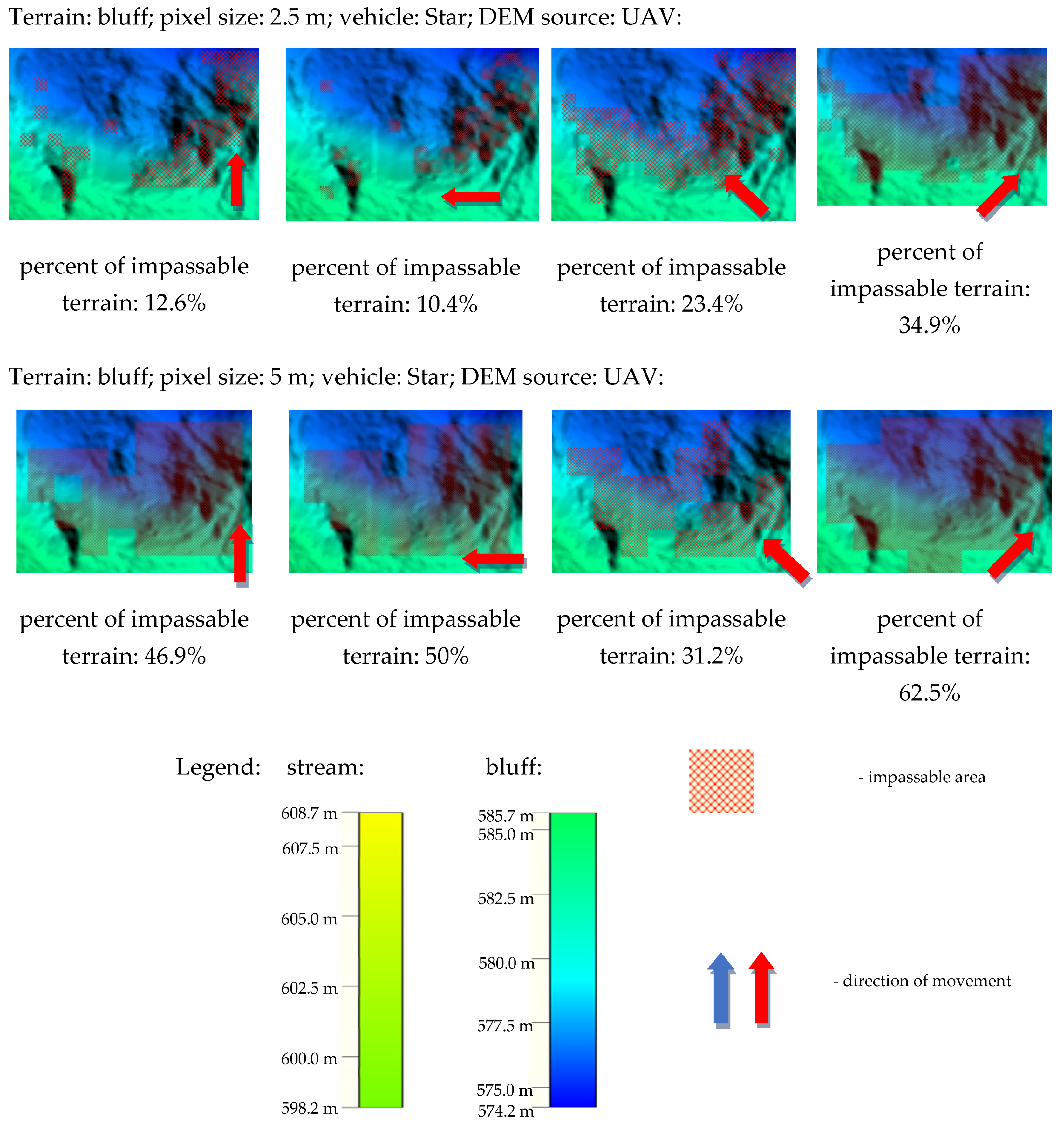
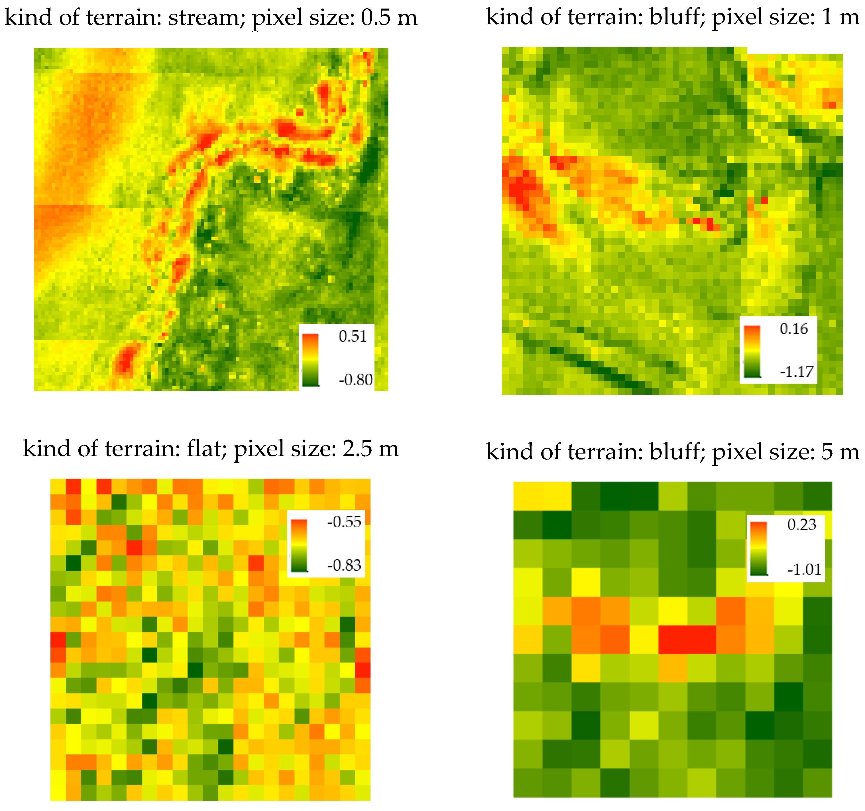
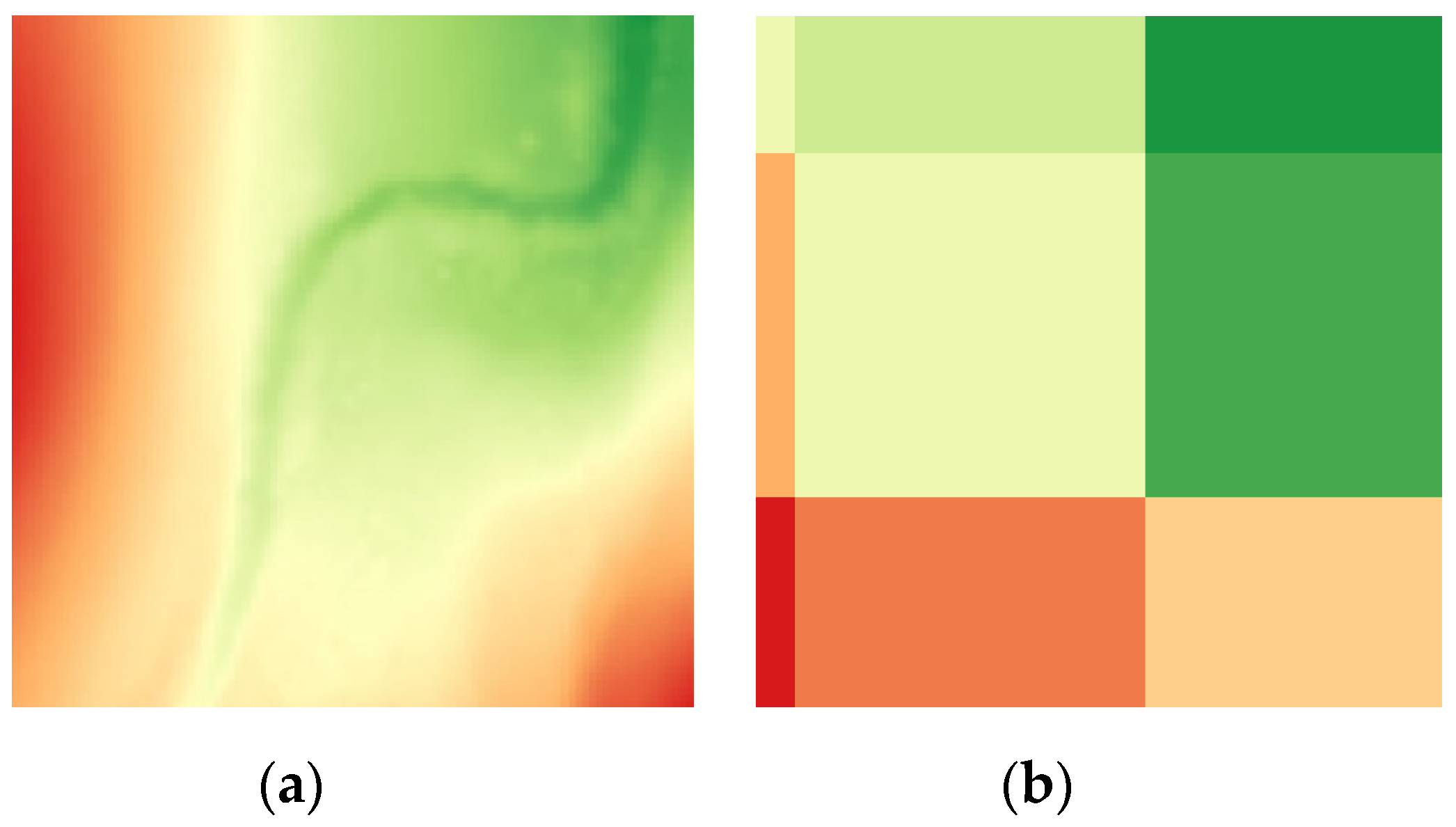
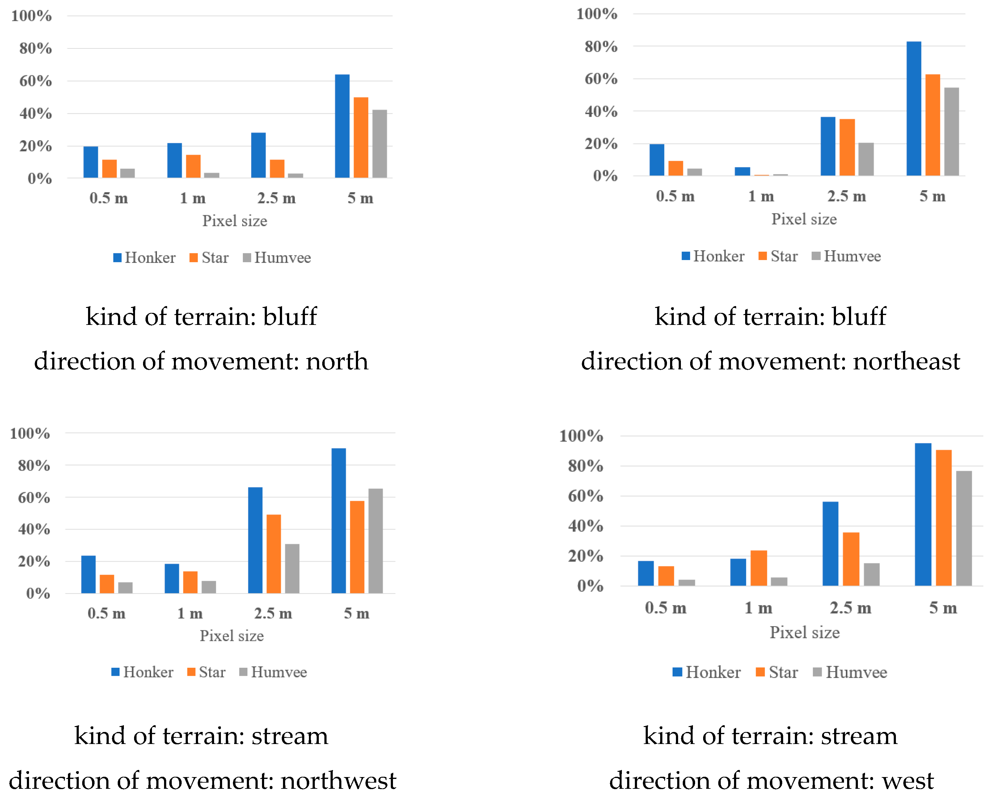
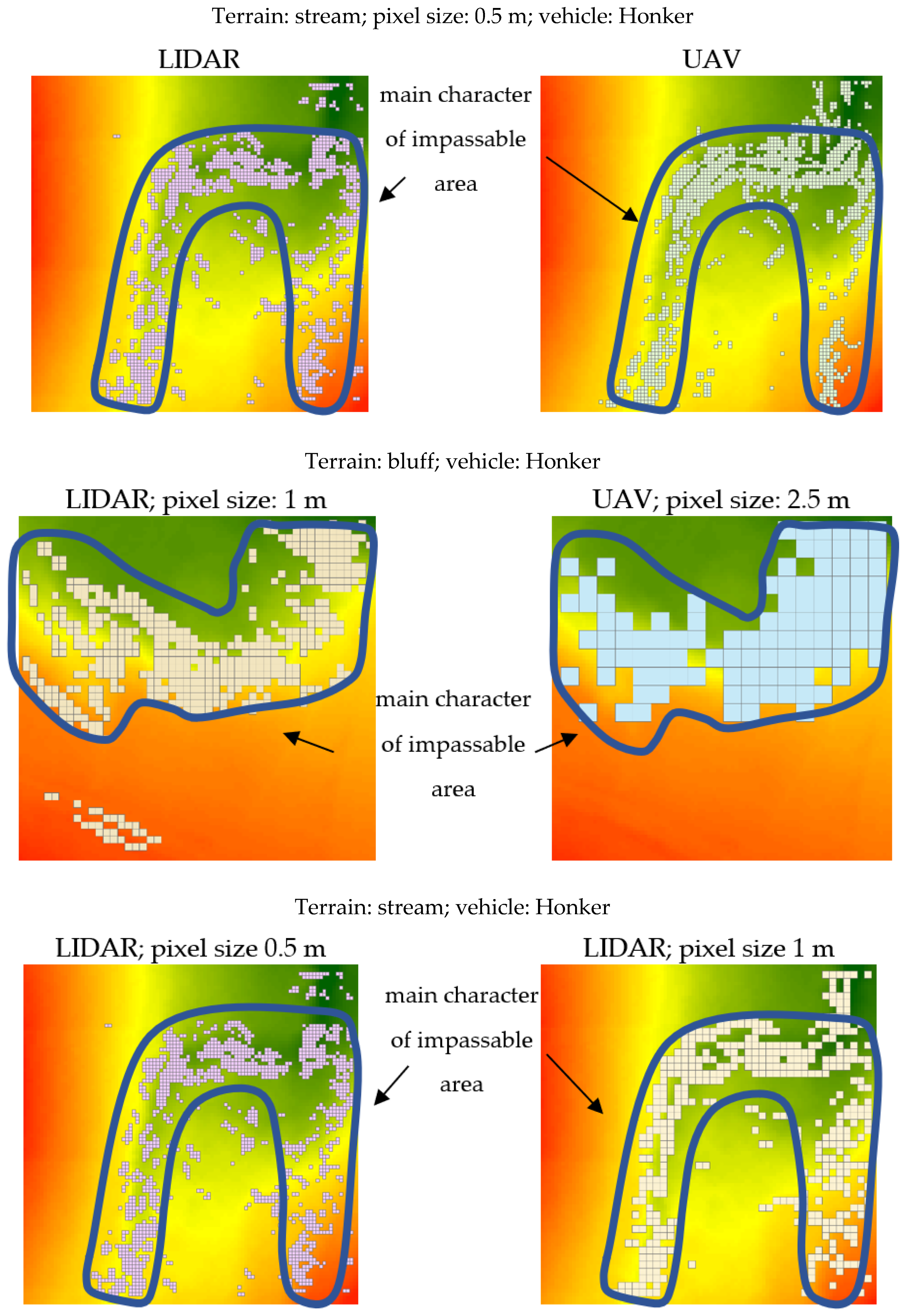
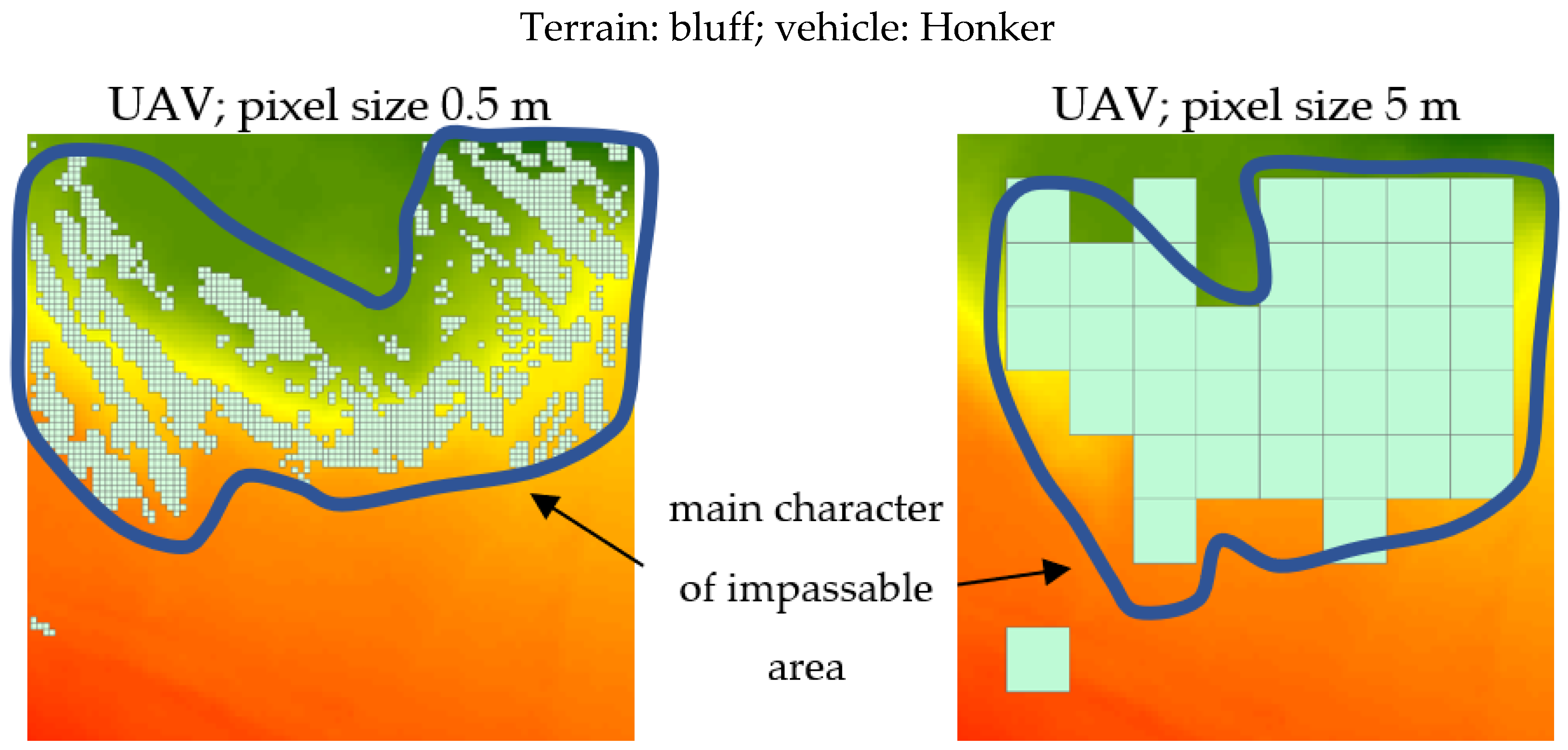
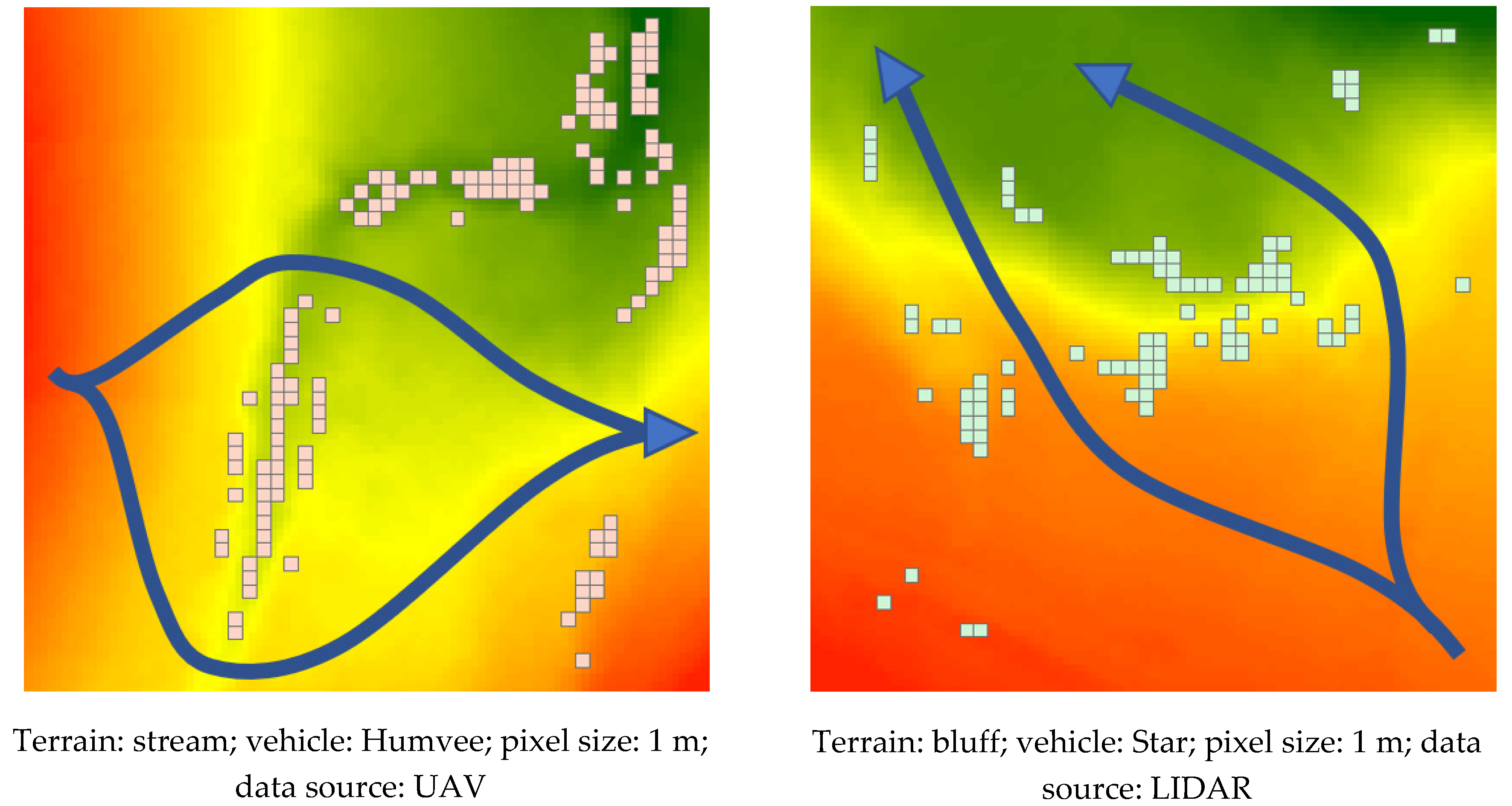
4. Results
5. Discussion
6. Conclusions
Author Contributions
Funding
Acknowledgments
Conflicts of Interest
Appendix A

References
- Ministry of National Defence. Defence Standard NO-06-A015:2012, Terrain—Rules of Classification—Terrain Analysis on Operational Level; Ministry of National Defence of Poland: Krakow, Poland, 2012.
- Department of the Army. Army Field Manual No. 5–33: Terrain Analysis; Headquarters Department of the Army: Washington, DC, USA, 1990. Available online: http://everyspec.com/ARMY/FM-Field-Manual/FM_5-33_13620/ (accessed on 30 October 2020).
- Balzter, H.; Cole, B.; Thiel, C.; Schmullius, C. Mapping CORINE land cover from Sentinel-1A SAR and SRTM digital elevation model data using random forests. Remote Sens. 2015, 7, 14876–14898. [Google Scholar] [CrossRef] [Green Version]
- Pennock, D.J.; Zebarth, B.J.; De Jong, E. Landform classification and soil distribution in hummocky terrain, Saskatchewan, Canada. Geoderma 1987, 40, 297–315. [Google Scholar] [CrossRef]
- Bielecka, E.; Jenerowicz, A.; Pokonieczny, K.; Borkowska, S. Land cover changes and flows in the Polish Baltic coastal zone: A qualitative and quantitative approach. Remote Sens. 2020, 12, 2088. [Google Scholar] [CrossRef]
- Pašakarnis, G.; Maliene, V. Towards sustainable rural development in Central and Eastern Europe: Applying land consolidation. Land Use Policy 2010, 27, 545–549. [Google Scholar] [CrossRef]
- Mościcka, A.; Pokonieczny, K.; Wilbik, A.; Wabiński, J. Transport accessibility of Warsaw: A case study. Sustainability 2019, 11, 5536. [Google Scholar] [CrossRef] [Green Version]
- Hošková-Mayerová, Š. Geospatial data reliability, their use in crisis situations. Int. Conf. Knowl. Based Organ. 2015, 21, 694–698. [Google Scholar] [CrossRef] [Green Version]
- Hubacek, M.; Ceplova, L.; Brenova, M.; Mikita, T.; Zerzan, P. Analysis of vehicle movement possibilities in terrain covered by vegetation. In Proceedings of the 2015 International Conference on Military Technologies (ICMT), Brno, Czech Republic, 19–21 May 2015; pp. 1–5. [Google Scholar] [CrossRef]
- Rybansky, M. Determination the ability of military vehicles to override vegetation. J. Terramech. 2020, 91, 129–138. [Google Scholar] [CrossRef]
- Rybansky, M. Modelling of the optimal vehicle route in terrain in emergency situations using GIS data. In 8th International Symposium of the Digital Earth; IOP Publishing Ltd.: Bristol, UK, 2014; Volume 18, p. 012131. [Google Scholar]
- Hubáček, M.; Rybansky, M.; Cibulova, K.; Brenov, M.; Ceplova, L. Mapping the passability of soils for vehicle movement. KVÜÕA Toim. 2016, 21, 5–18. [Google Scholar]
- Rybansky, M. Soil trafficability analysis. In Proceedings of the International Conference on Military Technologies (ICMT) 2015, Brno, Czech Repubic, 19–21 May 2015; pp. 1–5. [Google Scholar] [CrossRef]
- Hubáček, M.; Almášiová, L.; Dejmal, K.; Mertová, E. Combining different data types for evaluation of the soils passability. In The Rise of Big Spatial Data; Ivan, I., Singleton, A., Horák, J., Inspektor, T., Eds.; Springer International Publishing: Cham, Switzerland, 2017; pp. 69–84. [Google Scholar]
- Jayakumar, P.; Mechergui, D.; Wasfy, T.M. Understanding the effects of soil characteristics on mobility. In Proceedings of the 2017 International Design Engineering, Technical Conferences & Computers and Information in Engineering Conference, Cleveland, OH, USA, 6–9 August 2017. [Google Scholar] [CrossRef]
- McCullough, M.; Jayakumar, P.; Dasch, J.; Gorsich, D. The next generation NATO reference mobility model development. J. Terramech. 2017, 73, 49–60. [Google Scholar] [CrossRef]
- Bradbury, M.; Dasch, J.; Gonzalez, R.; Hodges, H.; Jain, A.; Iagnemma, K.; Letherwood, M.; McCullough, M.; Priddy, J. Next-Generation NATO Reference Mobility Model (NRMM) Development; Dasch, J., Jaykumar, P., Eds.; NATO: Bruxelles, Belgium, 2018. [Google Scholar]
- González, R.; Jayakumar, P.; Iagnemma, K. Stochastic mobility prediction of ground vehicles over large spatial regions: A geostatistical approach. Auton. Robot. 2017, 41, 311–331. [Google Scholar] [CrossRef]
- Gonzalez, R.; Jayakumar, P.; Iagnemma, K. An efficient method for increasing the accuracy of mobility maps for ground vehicles. J. Terramech. 2016, 68, 23–35. [Google Scholar] [CrossRef]
- Lessem, A.; Mason, G.; Ahlvin, R. Stochastic vehicle mobility forecasts using the nato reference mobility model. J. Terramech. 1996, 33, 273–280. [Google Scholar] [CrossRef]
- Maclaurin, B. Comparing the NRMM (VCI), MMP and VLCI traction models. J. Terramech. 2007, 44, 43–51. [Google Scholar] [CrossRef]
- Hofmann, A.; Hošková-Mayerová, Š.; Talhofer, V.; Kovařík, V. Creation of models for calculation of coefficients of terrain passability. Qual. Quant. 2014, 49, 1679–1691. [Google Scholar] [CrossRef]
- Rybansky, M.; Hofmann, A.; Hubacek, M.; Kovarik, V.; Talhofer, V. Modelling of cross-country transport in raster format. Environ. Earth Sci. 2015, 74, 7049–7058. [Google Scholar] [CrossRef] [Green Version]
- Pokonieczny, K.; Borkowska, S. Using high resolution spatial data to develop military maps of passability. In Proceedings of the 2019 International Conference on Military Technologies (ICMT), Brno, Czech Republic, 30–31 May 2019; pp. 1–8. [Google Scholar]
- Pokonieczny, K.; Mościcka, A. The influence of the shape and size of the cell on developing military passability maps. ISPRS Int. J. Geo Inf. 2018, 7, 261. [Google Scholar] [CrossRef] [Green Version]
- Pokonieczny, K. Automatic military passability map generation system. In Proceedings of the 2017 International Conference on Military Technologies (ICMT), Brno, Czech Republic, 31 May–2 June 2017; pp. 285–292. [Google Scholar]
- Pokonieczny, K. Use of a multilayer perceptron to automate terrain assessment for the needs of the armed forces. ISPRS Int. J. Geo Inf. 2018, 7, 430. [Google Scholar] [CrossRef] [Green Version]
- Rybansky, M. Effect of the Geographic Factors on the Cross Country Movement during Military Operations and the Natural Disasters; Rerucha, V., Ed.; University of Defence Brno: Brno, Czech Republic, 2007; ISBN 978-80-7231-238-2. [Google Scholar]
- Talhofer, V.; Hošková-Mayerová, Š.; Hofmann, A. Improvement of digital geographic data quality. Int. J. Prod. Res. 2012, 50, 4846–4859. [Google Scholar] [CrossRef]
- Richmond, P.W.; Mason, G.L.; Coutermarsh, B.A.; Pusey, J.; Moore, V.D. Mobility Performance Algorithms for Small Unmanned Ground Vehicles; Engineer Research and Development Center, Geotechnical and Structures Laboratory: Vicksburg, MS, USA, 2009. [Google Scholar]
- Shoop, S.; Knuth, M.; Wieder, W. Measuring vehicle impacts on snow roads. J. Terramech. 2013, 50, 63–71. [Google Scholar] [CrossRef]
- Ropero, F.; Muñoz, P.; R-Moreno, M.D. TERRA: A path planning algorithm for cooperative UGV–UAV exploration. Eng. Appl. Artif. Intell. 2019, 78, 260–272. [Google Scholar] [CrossRef]
- Hubacek, M.; Kovarik, V.; Kratochvil, V. Analysis of influence of terrain relief roughness on DEM accuracy generated from Lidar in the Czech Republic territory. ISPRS Int. Arch. Photogramm. Remote Sens. Spat. Inf. Sci. 2016, XLI-B4, 25–30. [Google Scholar] [CrossRef]
- Szombara, S.; Lewińska, P.; Żądło, A.; Róg, M.; Maciuk, K. Analyses of the Prądnik riverbed shape based on archival and contemporary data sets—Old maps, LiDAR, DTMs, orthophotomaps and cross-sectional profile measurements. Remote Sens. 2020, 12, 2208. [Google Scholar] [CrossRef]
- Wierzbicki, D. Multi-camera imaging system for UAV photogrammetry. Sensors 2018, 18, 2433. [Google Scholar] [CrossRef] [PubMed] [Green Version]
- Dohnal, F.; Hubacek, M.; Sturcova, M.; Bures, M.; Simkova, K. Identification of microrelief shapes along the line objects over DEM data and assessing their impact on the vehicle movement. In Proceedings of the 2017 International Conference on Military Technologies (ICMT), Brno, Czech Republic, 31 May–2 June 2017; pp. 262–267. [Google Scholar] [CrossRef]
- Dohnal, F.; Hubacek, M.; Simkova, K. Detection of microrelief objects to impede the movement of vehicles in terrain. ISPRS Int. J. Geo Inf. 2019, 8, 101. [Google Scholar] [CrossRef] [Green Version]
- Fryskowska, A.; Wróblewski, P. Mobile laser scanning accuracy assessment for the purpose of base-map updating. Geod. Cartogr. 2018, 67, 35–55. [Google Scholar] [CrossRef]
- Stereńczak, K.; Ciesielski, M.; Balazy, R.; Zawiła-Niedźwiecki, T. Comparison of various algorithms for DTM interpolation from LIDAR data in dense mountain forests. Eur. J. Remote Sens. 2016, 49, 599–621. [Google Scholar] [CrossRef]
- Head Office of Geodesy and Cartography. GUGiK Data PZGiK. Available online: http://www.gugik.gov.pl/pzgik (accessed on 21 October 2020).
- Starek, M.J. Light detection and ranging (LIDAR). In Encyclopedia of Estuaries; Encyclopedia of Earth Sciences Series; Springer: Dordrecht, The Netherlands, 2016; Volume 383. [Google Scholar] [CrossRef]
- Elprocus. LIDAR System (Light Detection and Ranging) Working and Applications; Elprocus: Hyderabad, India, 2019. [Google Scholar]
- ISOK. IT System for Country Protection Against Extreme Hazards (ISOK). Available online: https://isok.gov.pl/ (accessed on 30 October 2020).
- Lalak, M.; Wierzbicki, D.; Kędzierski, M. Methodology of processing single-strip blocks of imagery with reduction and optimization number of ground control points in UAV photogrammetry. Remote Sens. 2020, 12, 3336. [Google Scholar] [CrossRef]
- Sammartano, G.; Spanò, A. DEM generation based on UAV photogrammetry data in critical areas. In Proceedings of the 2nd International Conference on Geographical Information Systems Theory, Applications and Management, Rome, Italy, 26–27 April 2016; pp. 92–98. [Google Scholar] [CrossRef]
- Ajayi, O.G.; Salubi, A.A.; Angbas, A.F.; Odigure, M.G. Generation of accurate digital elevation models from UAV acquired low percentage overlapping images. Int. J. Remote Sens. 2017, 38, 3113–3134. [Google Scholar] [CrossRef]
- Sekrecka, A.; Wierzbicki, D.; Kedzierski, M. Influence of the sun position and platform orientation on the quality of imagery obtained from unmanned aerial vehicles. Remote Sens. 2020, 12, 1040. [Google Scholar] [CrossRef] [Green Version]
- Kedzierski, M.; Wierzbicki, D.; Sekrecka, A.; Fryskowska, A.; Walczykowski, P.; Siewert, J. Influence of lower atmosphere on the radiometric quality of unmanned aerial vehicle imagery. Remote Sens. 2019, 11, 1214. [Google Scholar] [CrossRef] [Green Version]
- Pepe, M.; Fregonese, L.; Scaioni, M. Planning airborne photogrammetry and remote-sensing missions with modern platforms and sensors. Eur. J. Remote Sens. 2018, 51, 412–436. [Google Scholar] [CrossRef]
- Roch, J.L. UAV classification and associated mission planning. In Multi-Rotor Platform-Based UAV Systems; ISTE: London, UK, 2020; pp. 27–44. ISBN 978-1-78548-251-9. [Google Scholar]
- LAS Dataset to Raster Function—Help ArcGIS for Desktop. Available online: https://desktop.arcgis.com/en/arcmap/10.3/manage-data/raster-and-images/las-dataset-to-raster-function.htm (accessed on 26 October 2020).
- LAS to Raster Function—Help ArcGIS for Desktop. Available online: https://desktop.arcgis.com/en/arcmap/10.3/manage-data/raster-and-images/las-to-raster-function.htm (accessed on 26 October 2020).
- Creating Raster DEMs and DSMs from Large Lidar Point Collections—Help ArcGIS Desktop. Available online: https://desktop.arcgis.com/en/arcmap/10.3/manage-data/las-dataset/lidar-solutions-creating-raster-dems-and-dsms-from-large-lidar-point-collections.htm (accessed on 26 October 2020).
- Wikipedia.pl. Honker; Wikipedia, the Free Encyclopaedia. Available online: https://pl.wikipedia.org/wiki/Honker (accessed on 20 October 2020).
- Brach, J. Star 266—Modernization. Available online: http://www.magnum-x.pl/artykul/star-266-projekty-modernizacji-czesc-ii (accessed on 20 October 2020).
- Military.com. High Mobility Multipurpose Wheeled Vehicle (HMMWV). Available online: https://www.military.com/equipment/high-mobility-multipurpose-wheeled-vehicle-hmmwv (accessed on 20 October 2020).
- Tyminski, Z. Vehicle 4x4 Honker 2000—User Manual 2008. Available online: http://honkerteam.pl/wp-content/uploads/2016/04/Instrukcja-Obs%C5%82ugi-HONKER-wrzesien-2008.pdf (accessed on 20 October 2020).
- Achilleos, G.A. The inverse distance weighted interpolation method and error propagation mechanism—Creating a DEM from an analogue topographical map. J. Spat. Sci. 2011, 56, 283–304. [Google Scholar] [CrossRef]
- Curran, P. Spatial autocorrelation. Appl. Geogr. 1989, 9, 138–139. [Google Scholar] [CrossRef]


| Translations | X (m) | Y (m) | Z (m) | Total (m) | ||
| 0.09 | 0.07 | 0.11 | 0.16 | |||
| Rotations | Omega (°/1000) | Phi (°/1000) | Kappa (°/1000) | |||
| 0.024 | 0.033 | 0.072 | ||||
| Source | Kind of Terrain | Pixel Size [m] | Minimum [m] | Maximum [m] | Average [m] | Standard Deviation |
|---|---|---|---|---|---|---|
| light detection and ranging (LIDAR) | bluff | 0.5 | −0.36 | 0.40 | 0.00 | 0.04 |
| 1 | −0.52 | 0.57 | 0.00 | 0.06 | ||
| 2.5 | −0.75 | 0.58 | 0.00 | 0.09 | ||
| 5 | −0.72 | 1.21 | 0.01 | 0.18 | ||
| stream | 0.5 | −0.47 | 0.39 | 0.00 | 0.05 | |
| 1 | −0.46 | 0.35 | 0.00 | 0.06 | ||
| 2.5 | −0.37 | 0.28 | 0.00 | 0.07 | ||
| 5 | −0.36 | 0.41 | 0.01 | 0.11 | ||
| flat | 0.5 | −0.10 | 0.11 | 0.00 | 0.02 | |
| 1 | −0.08 | 0.08 | 0.00 | 0.02 | ||
| 2.5 | −0.10 | 0.09 | 0.00 | 0.03 | ||
| 5 | −0.10 | 0.08 | 0.00 | 0.03 | ||
| unmanned aerial vehicle (UAV) | bluff | 0.5 | −0.28 | 0.19 | 0.00 | 0.02 |
| 1 | −0.56 | 0.12 | 0.00 | 0.03 | ||
| 2.5 | −0.49 | 0.18 | 0.00 | 0.05 | ||
| 5 | −0.19 | 0.31 | 0.02 | 0.09 | ||
| stream | 0.5 | −0.14 | 0.17 | 0.00 | 0.02 | |
| 1 | −0.19 | 0.27 | 0.00 | 0.03 | ||
| 2.5 | −0.35 | 0.41 | 0.00 | 0.07 | ||
| 5 | −0.31 | 0.70 | 0.03 | 0.16 | ||
| flat | 0.5 | −0.07 | 0.06 | 0.00 | 0.01 | |
| 1 | −0.06 | 0.06 | 0.00 | 0.01 | ||
| 2.5 | −0.09 | 0.07 | 0.00 | 0.02 | ||
| 5 | −0.06 | 0.06 | 0.00 | 0.02 |
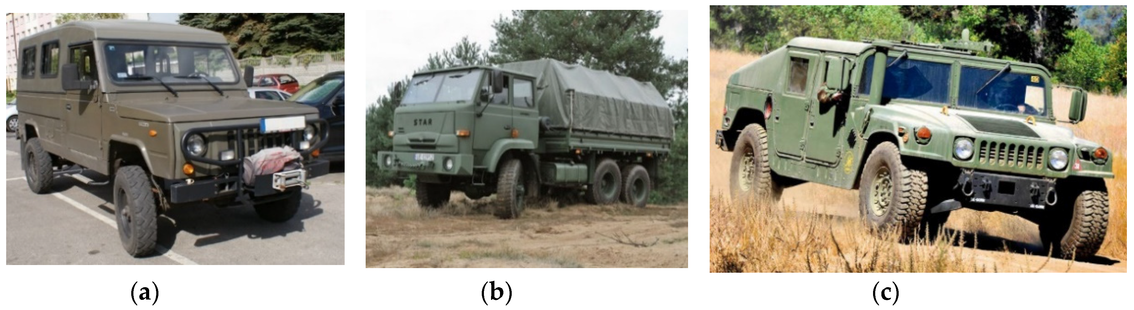
| Vehicle | Wheelbase (m) | Track Width (m) | Ground Clearance (m) | Approach Angle (°) | Descent Angle (°) |
|---|---|---|---|---|---|
| Honker | 2.90 | 1.65 | 0.22 | 40 | 40 |
| Star 266 | 2.99 | 2.00 | 0.33 | 37 | 42.5 |
| Humvee | 3.30 | 2.00 | 0.43 | 63 | 33 |
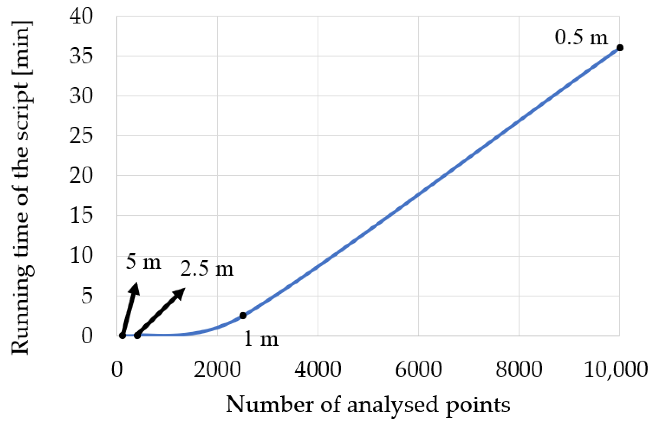
| Pixel Size (m) | Number of Grid Points in the Model | Execution Time |
|---|---|---|
| 0.5 | 10,000 | 36 min |
| 1 | 2500 | 2 min 30 s |
| 2.5 | 400 | 4 s |
| 5 | 100 | 1 s |
| Source | Pixel Size (m) | Minimum (m) | Maximum (m) | Average (m) | Standard Deviation | |
|---|---|---|---|---|---|---|
| bluff | LIDAR | 0.5 | 574.23 | 585.66 | 580.74 | 3.15 |
| 1 | 574.24 | 585.62 | 580.74 | 3.15 | ||
| 2.5 | 574.48 | 585.60 | 580.89 | 3.12 | ||
| 5 | 576.02 | 585.53 | 581.19 | 3.03 | ||
| UAV | 0.5 | 573.52 | 585.02 | 580.05 | 3.16 | |
| 1 | 573.54 | 584.96 | 580.05 | 3.16 | ||
| 2.5 | 574.00 | 584.98 | 580.25 | 3.11 | ||
| 5 | 575.22 | 584.87 | 580.45 | 3.05 | ||
| stream | LIDAR | 0.5 | 598.19 | 608.69 | 603.59 | 2.27 |
| 1 | 598.23 | 608.62 | 603.59 | 2.27 | ||
| 2.5 | 598.70 | 608.57 | 603.81 | 2.28 | ||
| 5 | 599.21 | 608.48 | 604.05 | 2.28 | ||
| UAV | 0.5 | 598.00 | 608.41 | 603.31 | 2.31 | |
| 1 | 598.11 | 608.34 | 603.31 | 2.31 | ||
| 2.5 | 598.68 | 608.38 | 603.55 | 2.31 | ||
| 5 | 598.96 | 608.25 | 603.77 | 2.32 | ||
| flat | LIDAR | 0.5 | 592.51 | 598.37 | 595.34 | 1.36 |
| 1 | 592.55 | 598.34 | 595.34 | 1.36 | ||
| 2.5 | 592.74 | 598.34 | 595.46 | 1.37 | ||
| 5 | 592.93 | 598.28 | 595.54 | 1.36 | ||
| UAV | 0.5 | 591.89 | 597.62 | 594.63 | 1.35 | |
| 1 | 591.92 | 597.59 | 594.63 | 1.35 | ||
| 2.5 | 592.06 | 597.57 | 594.72 | 1.36 | ||
| 5 | 592.25 | 597.53 | 594.81 | 1.36 |
| Honker Bluff Direction: N | Source | UAV | ||||||||
|---|---|---|---|---|---|---|---|---|---|---|
| Pixel Size | 0.5 m | 1 m | 2.5 m | 5 m | ||||||
| Source | Pixel Size | Impassable Terrain (m2) | 447 | 472 | 644 | 925 | ||||
| LIDAR | 0.5 m | 469 | 169 | 213 | 359 | 635 | ||||
| 191 | 278 | 210 | 259 | 184 | 285 | 179 | 290 | |||
| 1 m | 502 | 180 | 135 | 326 | 553 | |||||
| 235 | 267 | 165 | 337 | 184 | 318 | 130 | 372 | |||
| 2.5 m | 638 | 161 | 131 | 119 | 394 | |||||
| 352 | 286 | 297 | 341 | 113 | 525 | 107 | 531 | |||
| 5 m | 1025 | 142 | 99 | 138 | 25 | |||||
| 720 | 305 | 652 | 373 | 214 | 506 | 125 | 900 | |||
| Honker Bluff Direction: N | Source | LIDAR | ||||||||
|---|---|---|---|---|---|---|---|---|---|---|
| Pixel Size | 0.5 m | 1 m | 2.5 m | 5 m | ||||||
| Source | Pixel Size | Impassable Terrain (m2) | 469 | 502 | 638 | 1025 | ||||
| LIDAR | 0.5 m | 469 | 138 | |||||||
| 138 | 331 | |||||||||
| 1 m | 502 | 159 | 0 | |||||||
| 192 | 310 | 0 | 502 | |||||||
| 2.5 m | 638 | 185 | 171 | 0 | ||||||
| 354 | 284 | 307 | 331 | 0 | 638 | |||||
| 5 m | 1025 | 157 | 118 | 107 | 0 | |||||
| 713 | 312 | 641 | 384 | 494 | 531 | 0 | 1025 | |||
| Honker Bluff Direction: N | Source | UAV | ||||||||
|---|---|---|---|---|---|---|---|---|---|---|
| Pixel Size | 0.5 m | 1 m | 2.5 m | 5 m | ||||||
| Source | Pixel Size | Impassable Terrain (m2) | 447 | 472 | 644 | 925 | ||||
| UAV | 0.5 m | 447 | 0 | |||||||
| 0 | 447 | |||||||||
| 1 m | 472 | 150 | 0 | |||||||
| 175 | 297 | 0 | 472 | |||||||
| 2.5 m | 644 | 157 | 136 | 0 | ||||||
| 354 | 290 | 308 | 336 | 0 | 644 | |||||
| 5 m | 925 | 156 | 109 | 144 | 0 | |||||
| 634 | 291 | 562 | 363 | 425 | 500 | 0 | 925 | |||
| Honker Stream Direction: N | Source | UAV | ||||||||
|---|---|---|---|---|---|---|---|---|---|---|
| Pixel Size | 0.5 m | 1 m | 2.5 m | 5 m | ||||||
| Source | Pixel Size | Impassable Terrain (m2) | 350 | 408 | 1225 | 1550 | ||||
| LIDAR | 0.5 m | 344 | 178 | 222 | 1021 | 1298 | ||||
| 172 | 172 | 158 | 186 | 140 | 204 | 92 | 252 | |||
| 1 m | 426 | 164 | 157 | 953 | 1219 | |||||
| 240 | 186 | 175 | 251 | 154 | 272 | 95 | 331 | |||
| 2.5 m | 1375 | 96 | 70 | 100 | 525 | |||||
| 1121 | 254 | 1037 | 338 | 250 | 1125 | 350 | 1025 | |||
| 5 m | 1525 | 89 | 76 | 275 | 75 | |||||
| 1264 | 261 | 1193 | 332 | 575 | 950 | 50 | 1475 | |||
| Honker Stream Direction: N | Source | LIDAR | ||||||||
|---|---|---|---|---|---|---|---|---|---|---|
| Pixel Size | 0.5 m | 1 m | 2.5 m | 5 m | ||||||
| Source | Pixel Size | Impassable Terrain (m2) | 344 | 426 | 1375 | 1525 | ||||
| LIDAR | 0.5 m | 344 | 0 | |||||||
| 0 | 344 | |||||||||
| 1 m | 426 | 132 | 0 | |||||||
| 214 | 212 | 0 | 426 | |||||||
| 2.5 m | 1375 | 88 | 90 | 0 | ||||||
| 1119 | 256 | 1039 | 336 | 0 | 1375 | |||||
| 5 m | 1525 | 80 | 76 | 294 | 0 | |||||
| 1261 | 264 | 1173 | 352 | 444 | 1081 | 0 | 1525 | |||
| Honker Stream Direction: N | Source | UAV | ||||||||
|---|---|---|---|---|---|---|---|---|---|---|
| Pixel Size | 0.5 m | 1 m | 2.5 m | 5 m | ||||||
| Source | Pixel Size | Impassable Terrain (m2) | 350 | 408 | 1225 | 1550 | ||||
| UAV | 0.5 m | 350 | 0 | |||||||
| 0 | 350 | |||||||||
| 1 m | 408 | 126 | 0 | |||||||
| 184 | 224 | 0 | 408 | |||||||
| 2.5 m | 1225 | 150 | 141 | 0 | ||||||
| 1025 | 200 | 958 | 267 | 0 | 1225 | |||||
| 5 m | 1550 | 106 | 106 | 287 | 0 | |||||
| 1306 | 244 | 1248 | 302 | 612 | 938 | 0 | 1550 | |||
| Pixel Size (m) | Bluff | Stream | ||
|---|---|---|---|---|
| LIDAR | UAV | LIDAR | UAV | |
| 0.5 | 0.68 | 0.70 | 0.61 | 0.64 |
| 1 | 0.80 | 0.82 | 0.76 | 0.81 |
| 2.5 | 0.93 | 0.93 | 0.92 | 0.92 |
| 5 | 0.96 | 0.96 | 0.95 | 0.95 |
Publisher’s Note: MDPI stays neutral with regard to jurisdictional claims in published maps and institutional affiliations. |
© 2020 by the authors. Licensee MDPI, Basel, Switzerland. This article is an open access article distributed under the terms and conditions of the Creative Commons Attribution (CC BY) license (http://creativecommons.org/licenses/by/4.0/).
Share and Cite
Dawid, W.; Pokonieczny, K. Analysis of the Possibilities of Using Different Resolution Digital Elevation Models in the Study of Microrelief on the Example of Terrain Passability. Remote Sens. 2020, 12, 4146. https://0-doi-org.brum.beds.ac.uk/10.3390/rs12244146
Dawid W, Pokonieczny K. Analysis of the Possibilities of Using Different Resolution Digital Elevation Models in the Study of Microrelief on the Example of Terrain Passability. Remote Sensing. 2020; 12(24):4146. https://0-doi-org.brum.beds.ac.uk/10.3390/rs12244146
Chicago/Turabian StyleDawid, Wojciech, and Krzysztof Pokonieczny. 2020. "Analysis of the Possibilities of Using Different Resolution Digital Elevation Models in the Study of Microrelief on the Example of Terrain Passability" Remote Sensing 12, no. 24: 4146. https://0-doi-org.brum.beds.ac.uk/10.3390/rs12244146