Using GRACE Data to Study the Impact of Snow and Rainfall on Terrestrial Water Storage in Northeast China


1
School of Ecology and Environment, Institute of Disaster Prevention, Sanhe 065201, China
2
Hebei Key Laboratory of Earthquake Dynamics, Institute of Disaster Prevention, Sanhe 065201, China
3
Institute of Geodesy, University of Stuttgart, Stuttgart 70174, Germany
4
College of Geodesy and Geomatics, Shandong University of Science and Technology, Qingdao 266590, China
*
Author to whom correspondence should be addressed.
Remote Sens. 2020, 12(24), 4166; https://0-doi-org.brum.beds.ac.uk/10.3390/rs12244166
Submission received: 13 November 2020
/
Revised: 16 December 2020
/
Accepted: 18 December 2020
/
Published: 19 December 2020
(This article belongs to the Special Issue GRACE Satellite Gravimetry for Geosciences)
Abstract
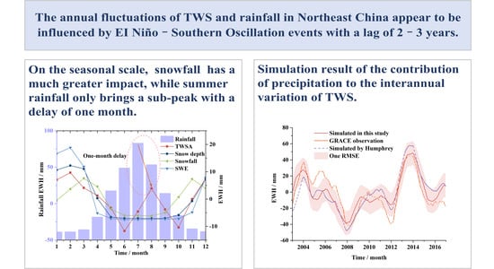
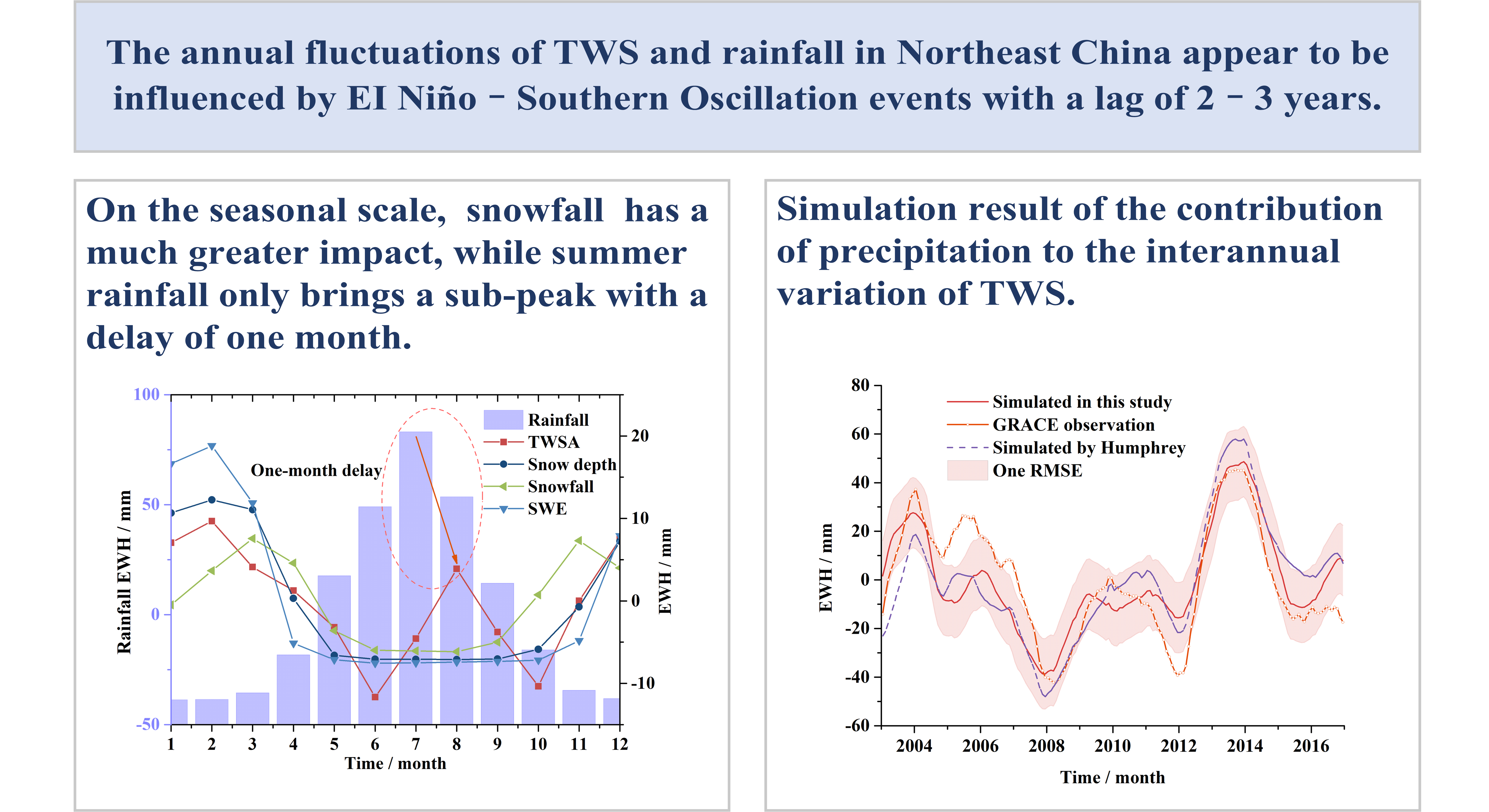
:Water resources are important for agricultural, industrial, and urban development. In this paper, we analyzed the influence of rainfall and snowfall on variations in terrestrial water storage (TWS) in Northeast China from Gravity Recovery and Climate Experiment (GRACE) gravity satellite data, GlobSnow snow water equivalent product, and ERA5-land monthly total precipitation, snowfall, and snow depth data. This study revealed the main composition and variation characteristics of TWS in Northeast China. We found that GRACE provided an effective method for monitoring large areas of stable seasonal snow cover and variations in TWS in Northeast China at both seasonal and interannual scales. On the seasonal scale, although summer rainfall was 10 times greater than winter snowfall, the terrestrial water storage in Northeast China peaked in winter, and summer rainfall brought about only a sub-peak, 1 month later than the maximum rainfall. On the interannual scale, TWS in Northeast China was controlled by rainfall. The correlation analysis results revealed that the annual fluctuations of TWS and rainfall in Northeast China appear to be influenced by ENSO (EI Niño–Southern Oscillation) events with a lag of 2–3 years. In addition, this study proposed a reconstruction model for the interannual variation in TWS in Northeast China from 2003 to 2016 on the basis of the contemporary terrestrial water storage and rainfall data.
1. Introduction
Terrestrial water storage (TWS) is an important component of the global hydrological cycle system and plays a key role in the Earth’s climate system [1,2,3]. Water resources are the basis of agricultural, industrial, and urban development. Therefore, the study of water reserves has a high social value and great scientific research significance. In terms of the vertical spatial distribution of water storage, TWS is the sum of surface water, snow, ice, soil water storage, and groundwater [4]. In addition, changes in TWS are an integrated reflection of activities such as precipitation, evaporation, runoff, and groundwater [5]. Traditional means of observing TWS mainly rely on ground-based hydrological stations (such as observation wells) and terrestrial hydrological models (such as Global Land Data Assimilation System (GLDAS) model [6]). Hydrological station observations are susceptible to the limitations of uneven spatial distribution of stations. TWS measurements taken at a single location can hardly be representative of the entire interest area [7]. Therefore, observation wells can provide high-resolution estimates of groundwater storage (GWS) in localized areas, but they struggle to measure regional GWS in mountainous areas or arid regions [8,9]. Terrestrial hydrological models are also limited to specific hydrological elements. For instance, outputs of the GLDAS model only contain the near-surface soil water content variations, which do not reflect the entire water storage variations from surface to subsurface [10,11]; unlike the GLDAS model, the Australian Water Resources Assessment (AWRA) model includes a groundwater component, while it does not account for human activities, such as large amounts of water pumped during times of drought [7]. Thus, traditional observations and models have their own limitations in the understanding of terrestrial hydrology.
The Gravity Recovery and Climate Experiment (GRACE) gravity satellite, designed by the United States and Germany, was launched in March 2002. It can be used to monitor the global large-scale time-varying gravity field [12,13,14]. The GRACE satellite provides an efficient method to observe time-varying gravity fields, which can be used for a variety of applications. For instance, the seismic gravity field changes as a result of large subduction earthquakes [15,16], mass change in polar ice sheet and global high mountain glaciers [17,18,19], global mean sea level change as a response to global warming [20], changes in sediment deposition rates in coastal areas [21], and determination of surface mass with correction of the Earth’s oblateness effect [22,23]. In the context of TWS monitoring, GRACE provides an effective means of monitoring changes in TWS at global, regional, and basin scales [24,25]. The TWS changes quantified by GRACE data represent the sum of surface water and groundwater, with accuracies approaching a few millimeters in water height over land [12]. Previous studies of TWS have mostly focused on the following aspects: determination of seasonal, interannual, and trend changes in TWS [26,27,28]; isolation and interpretation of widespread groundwater deficits and ground subsidence in conjunction with GRACE data, hydrological models, and field measurements [24,25,29,30,31]; improving the accuracy of GRACE data for groundwater estimation [7]; and analysis and interpretation of the impact of extreme climate events (i.e., ENSO—EI Niño-Southern Oscillation) on global or regional TWS [32,33,34,35].
However, TWS is primarily controlled by activities such as rainfall, snowfall, runoff, and groundwater discharge. In the equatorial or non-high-altitude regions of the middle and low latitudes (between 40° and 55°), due to the absence of significant seasonal snow cover, TWS is mainly controlled by precipitation and runoff. In contrast, in middle- and high-latitude regions, snowfall and snow cover account for a large proportion of TWS under conditions of reduced evaporation and runoff activity in winter. An accurate understanding of the composition of water reserves is a prerequisite for the proper analysis of TWS observations and rational planning of water resources. Although remote sensing satellites using microwave or visible spectrum imagery can be used to derive the spatial distribution of snow cover and estimate the amount of snow picks [36,37,38], these approaches rely on indirect estimates for retrieving snow parameters, which can be significantly affected by atmosphere (i.e., cloud pollution effects on optical imagery), climatic conditions (i.e., temperature effects on snow density), land surface (i.e., vegetation), and snow cover thickness [39]. In contrast to the remote sensing methods described above, GRACE observations eliminate most of the limitations of these conditions [40]. The GRACE satellite has been used to assess the evolution of snow mass at high latitudes [41], separate SWE (snow water equivalent) from other TWS components [42], and assimilate terrestrial water storage in a snow-dominated basin [43]. All these studies validated the ability of GRACE to monitor snow mass. Nevertheless, the contribution of snow to TWS in China is still poorly quantified.
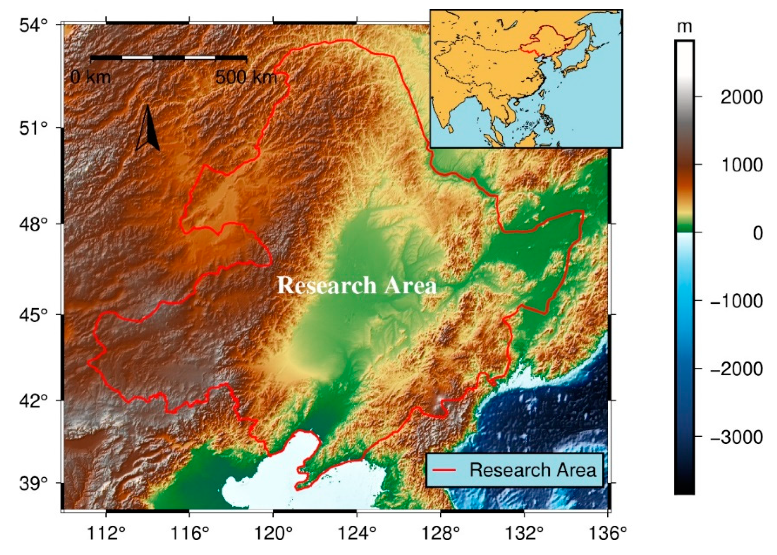
To date, the studies of snow cover in China have focused on the following areas: the temporal and spatial distribution characteristics of snow [44,45,46]; the effects of topography, elevation, and location on snow cover variation [47]; and the combination of GRACE and hydrological model data to study groundwater storage changes and regional drought phenomena [35,48]. Northeast China (Figure 1), with winter temperatures below −11 °C, is a region with extensive and stable snow cover. The area of Northeast China is approximately 1.45 million km2, which is well within the nominal resolution of the GRACE data (about 0.1 million km2). In winter, snowfall is frequent and evenly distributed, and snow cover lasts from November until April of the following year [44]. There have been few systematic studies of rainfall and snowfall on TWS changes in Northeast China thus far.
In this paper, we combined GRACE satellite data, snow cover, snowfall, rainfall, and snow depth data to investigate the ability of GRACE data to monitor large-scale snow cover and the impact of rainfall and snowfall on terrestrial water storage in Northeast China. The main research objectives are as follows: (1) to understand the impact of rainfall and snowfall on seasonal changes in terrestrial water storage anomalies (TWSA), (2) to understand the impact of ENSO on rainfall and TWSA, (3) to simulate TWS changes from 2003 to 2016 in Northeast China on the basis of the new insights, and (4) to understand the challenges in investigating snow cover mass change by using GRACE data and uncertainties in the impact of ENSO on rainfall and TWS.
2. Data and Methods
2.1. GRACE Data
We used the monthly Release 06 solutions, with spherical harmonic coefficients truncated to degree 60, provided by JPL (the Jet Propulsion Laboratory), CSR (the Center for Space Research at the University of Texas at Austin), and GFZ (the German Geosciences Research Center) (http://icgem.gfz-potsdam.de/series). The GRACE monthly Release 06 solutions provided by JPL, CSR, and GFZ were averaged January 2003 – December 2016). The spherical harmonic coefficients were treated as follows: the C20s coefficients were replaced by the satellite laser ranging solutions [49]; the degree-1 coefficients were added back according to GRACE Technical Note 13 [50], which were computed on the basis of the data of Sun et al. [51]; the GIA (glacial isostatic adjustment) effect was corrected by a three-dimensional model on the basis of the data of Geruo et al. [52]. The spherical harmonic coefficients were filtered using the DDK4 method [53]. Then, Equation (1) [12] was used to calculate the gridded TWSA. The time series of TWSA in Northeast China was calculated by using an area-based weighting method.
where is the variation of equivalent water height (EWH), and a are the mean density and radius of the Earth, θ and λ are geocentric colatitude and geocentric longitude, l represents the degree of the spherical harmonic coefficients, m represents the order of the spherical harmonic coefficients, kl is the Load Love number at degree l [54], is the fully normalized Legendre function of degree l and order m, and and are the residual fully normalized spherical harmonic coefficients relative to the average gravity field between 2005 and 2010.
2.2. GlobSnow Snow Water Equivalent Products
The GlobSnow project, funded by the ESA (European Space Agency), has well-known precision characteristics and aims to create temporally and spatially extensive snow products [55]. The framework of GlobSnow project produces 2 snow parameter products, snow water equivalent (SWE) and snow extent (SE) [55]. The SWE information for terrestrial covers the area between 35° N and 85° N, excluding Greenland and glaciers [55]. The GlobSnow SWE product is projected onto the Equal Area Scalable Earth Grid (EASE-Grid) with a nominal resolution of 25 × 25 km for a single pixel [55]. It has a higher accuracy than the AMSR-2 and FY-3B products [56]. In this paper, we used monthly GlobSnow v3.0 SWE data ( January 2003 – December 2016) to validate the snow depth data (http://www.globsnow.info/swe/archive_v3.0/L3B_monthly_SWE/). The SWE data were treated as follows: (1) the projected SWE product was described in a plane coordinate system (x, y, f: x and y are the locations of SWE in plane coordinate system, f is the value of SWE), while the TWSA calculated by GRACE was described in a geodesic coordinate system, and thus the projection transformation method was needed to convert SWE product to be described in geographic coordinates (L, B, f: L and B are the locations of SWE in the geographic coordinate system, f is the value of SWE); (2) the cubic polynomial interpolation method was used to impute the SWE product to a 1° × 1° grid; (3) to unify the spatial resolution of SWE and TWSA, we calculated SWE data in spherical harmonics using the same cut-off degree (60) and DDK4 filter method as for GRACE, and then derived it into product expressed as equivalent water height. The time series of SWE in Northeast China was calculated by using an area-based weighting method.
2.3. Average Monthly Data of ERA5-Land
ERA5-Land is a reanalysis dataset produced by the ECMWF ERA5 climate reanalysis model. The dataset includes monthly dynamic data since 1981, which contains 50 indicators characterizing temperature, lakes, snowpack, soil moisture, radiation and heat, evaporation and runoff, wind speed, barometric pressure, precipitation, and vegetation. Compared to ERA5, it provides a consistent view of the evolution of land variables over several decades at a much higher resolution (approximately 9 × 9 km, 0.1° × 0.1°) [57]. It mainly consists of 2 datasets, ERA5-Land hourly data and ERA5-Land monthly averaged data. We used monthly average reanalysis data of snowfall, snow depth, and total precipitation (TP; includes snow and rainfall) downloaded from the Climate Data Store (CDS) (https://cds.climate.copernicus.eu/cdsapp#!/home) for the period 1981–2016 [58]. All data provided by CDS are expressed as EWH. As mentioned in Section 2.2, we should unify the spatial resolution with the rest of the paper. Snowfall, snow depth, and total precipitation data were treated as follows: (1) the monthly average reanalysis snowfall, snow depth, and total precipitation data provided by CDS are the daily average for the month, and thus they should be multiplied by the number of days in the month; (2) we used the average accumulation method to impute snowfall, snow depth, and total precipitation data to a 1° × 1° grid; (3) we calculated these data in spherical harmonics using the same cut-off degree (60) and DDK4 filter method as for GRACE, and then derived them into products expressed as equivalent water height. The time series of snowfall, snow depth, and rainfall (TP minus snowfall) in Northeast China was calculated by using an area-based weighting method.
2.4. SOI
The Southern Oscillation Index (SOI) shows the development and intensity of El Niño and La Niña events in the Pacific Ocean. It can be calculated using the pressure differences between Tahiti and Darwin. Sustained negative SOI values below −7 typically indicate an El Niño phenomenon, while sustained positive SOI values greater than +7 indicate a typical La Niña phenomenon [59]. In this paper, the SOI data were provided by the Bureau of Meteorology of the Australian Government (ftp://ftp.bom.gov.au/anon/home/ncc/www/sco/soi/soiplaintext.html). We used it to investigate the effect of the ENSO events on interannual variations in Northeast China.
2.5. Fitting Method
Prior research has generally assumed that TWS and precipitation are the sums of linear variations, interannual variations, and semi-annual variations [32]. To obtain the phase and amplitude of TWSA, snowfall, rainfall, snow depth, and SWE, we used the least squares method to fit these time series. The annual and semi-annual cycles were also considered in the following equation [60]:
where a is the constant, b is the trend, c and d are the annual and semi-annual amplitudes, x is the time, T1 and T2 are the annual and semi-annual cycles, φ1 and φ2 are the initial phases, and ε is the residual error.
2.6. Methods for Separating Interannual and Seasonal Signals
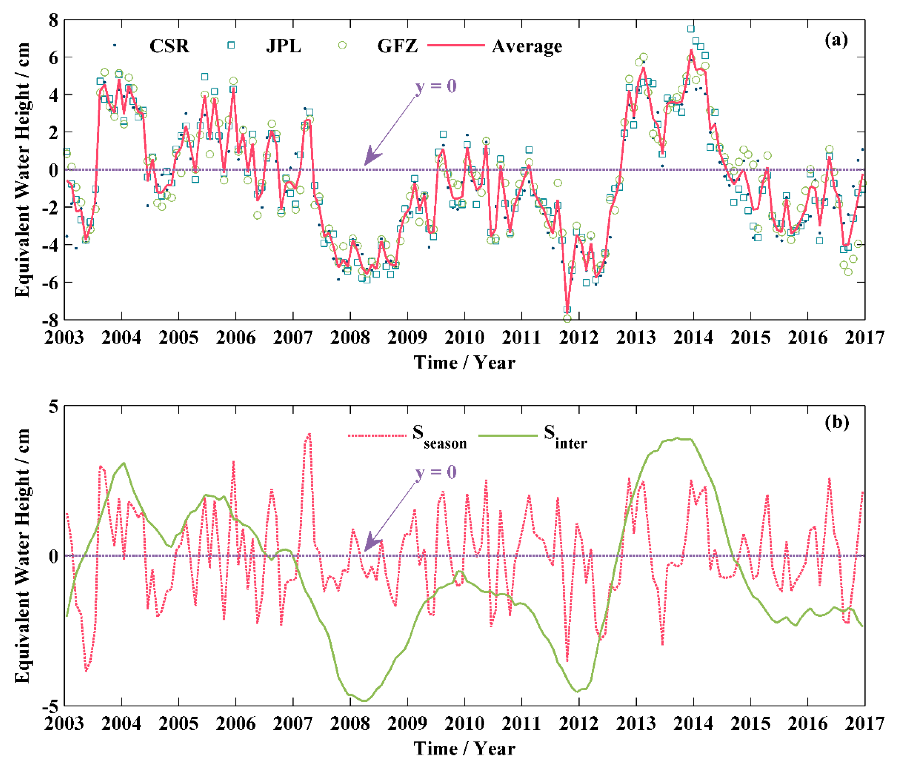
TWSA, SWE, snowfall, snow depth, and total precipitation (TP; includes snowfall and rainfall) data were all expressed in EWH. Figure 2a shows the time series of TWSA estimated using CSR, JPL, and GFZ solutions and their average. Figure 3 shows the time series of SWE, snowfall, snow depth, and rainfall. As shown in Figure 2a, we can tentatively conclude that TWSA series contained significant interannual variations with a greater amplitude than seasonal variations. In order to investigate interannual and seasonal components separately, we used a sliding average method to separate interannual and seasonal signals [4]. The original TWSA, SWE, snowfall, snow depth, and TP time series (S0) were averaged over a sliding 12-month window to obtain the interannual variation time series (Sinter). For terminal observations, we used all available observations for the average. The seasonal variation (Sseason) time series were obtained through S0 − Sinter, as shown in Equation (3). Figure 2b shows that TWSA contained evident interannual and seasonal signals and confirms that signal separation is necessary.
3. Results
3.1. Impact of Rainfall and Snowfall on Seasonal Changes in TWSA in Northeast China
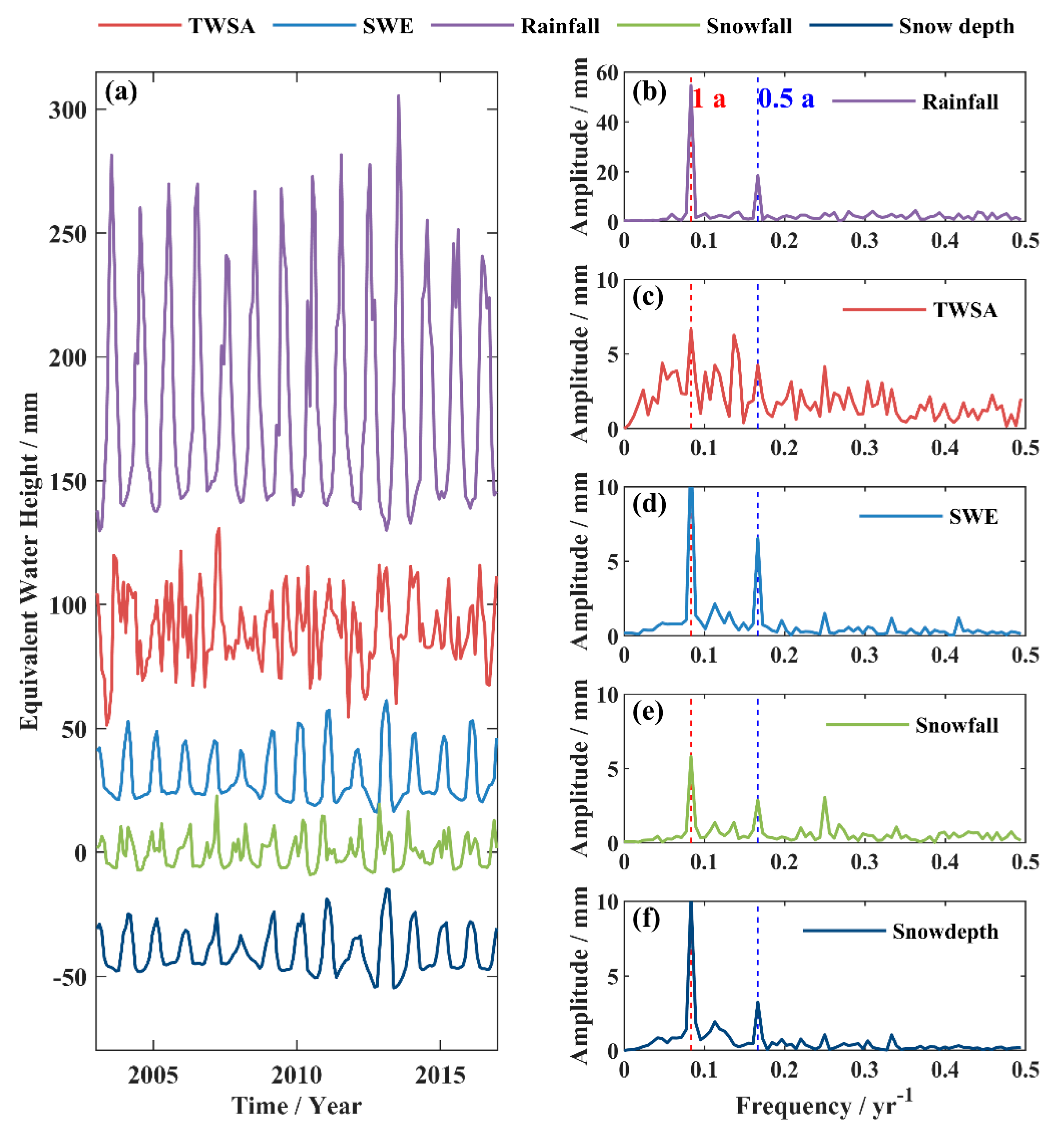
Figure 4a shows the time series of seasonal TWSA, rainfall, snowfall, and snow depth in Northeast China. Combined with the spectral analysis results (Figure 4b–f), it can be seen that the time series of seasonal changes of snowfall, snow depth, and rainfall had strong annual and semi-annual cycles. To analyze seasonal signals in detail, we used Equation (2) to fit the TWSA, SWE, snowfall, snow depth, and rainfall seasonal variation time series. On the basis of the adjustment of the indirect observations model [61], we estimated the coefficients of Equation (2) and then estimated the annual amplitudes and annual phases of seasonal time series of TWSA, rainfall, snowfall, snow depth, and SWE with their root mean square errors (RMSEs). Table 1 shows that the largest annual amplitude of rainfall was about 56.64 mm; the annual amplitude of TWSA was similar to snowfall, about 6–7 mm; the annual amplitude of snow cover was consistent with snow depth, about 10–12 mm; and there was good consistency among annual phase of snowfall, snow cover, snow depth, and TWSA (annual amplitude peaked around January, with RMSE of annual phases below 0.5 months). However, the seasonal amplitude of rainfall was about eight times greater than that of TWSA. We speculate that this was because the increase in rainfall is largely offset by the corresponding increase in evapotranspiration and runoff on seasonal time scales. Northeast China is characterized by a temperate monsoon climate. Rainfall is concentrated in July and August, and snowfall dominates the winter when evapotranspiration and runoff are weakened; hence, TWS is susceptible to snowfall. The difference in sensitivity to rainfall and snowfall explains the different agreement in the results of phase (~1 year) and amplitude (6–12 mm) of snow depth, snowfall, and TWSA. The RMSE values for TWSA, rainfall, snowfall, snow depth and SWE annual amplitudes were 2.16, 2.17, 0.64, 0.60, and 0.65 mm, respectively. Comparing these RMSE values with their annual amplitudes, we found the relative RMSE (RMSE/amplitude) of rainfall, snowfall, snow depth, and SWE to be about 4%, 11%, 6%, and 5%, respectively, while the relative RMSE of TWSA reached 33%. It is clear that the seasonal term of TWSA is less reliable (Figure 4c).
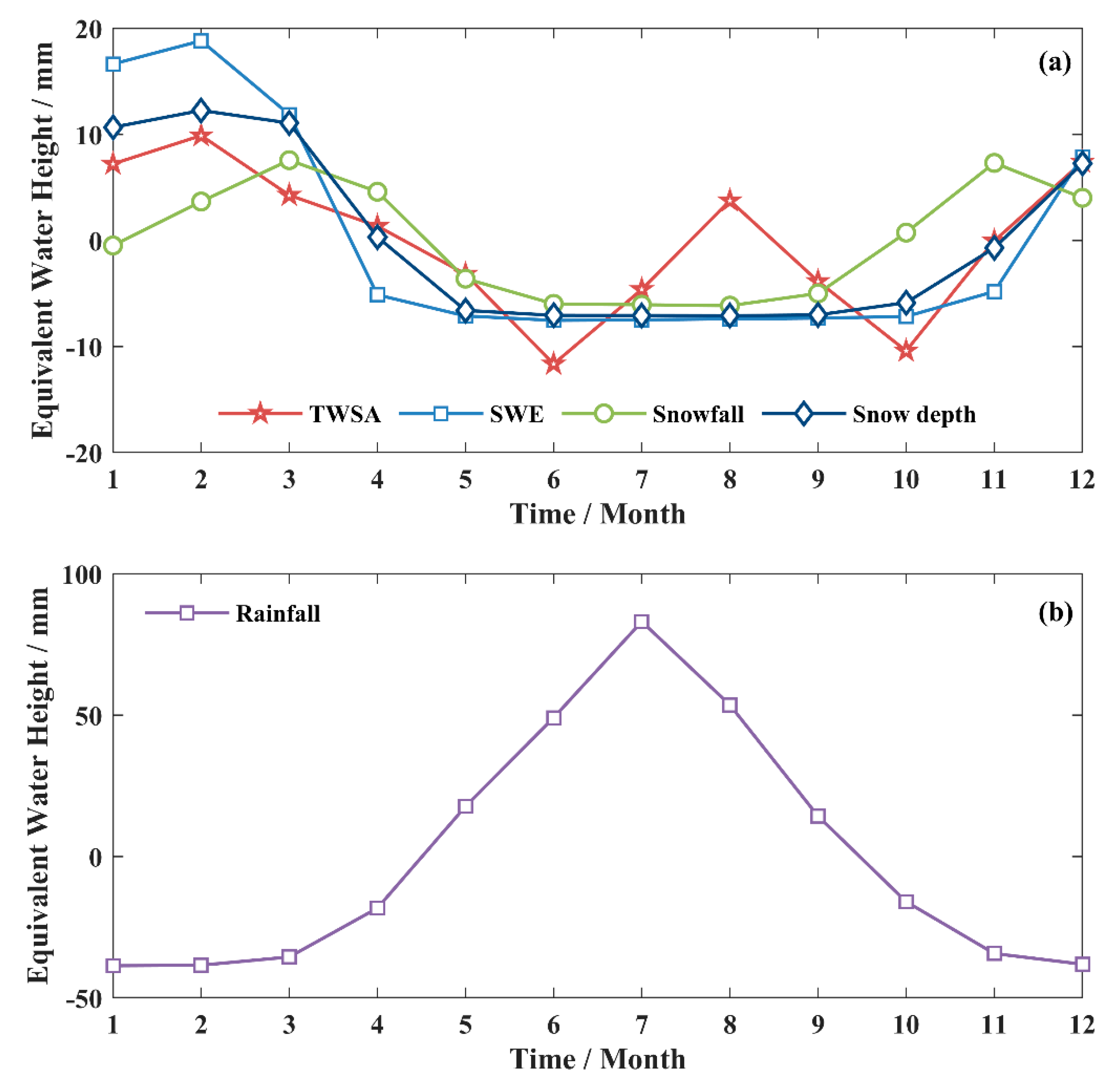
In order to further analyze the influence of rainfall and snowfall on TWSA at the seasonal scale, we averaged the seasonal variation time series of 2003 to 2016 (Figure 5) by month to obtain the monthly mean variation. The monthly mean variations in rainfall, SWE, snowfall, and snow depth were generally consistent with the climate characteristics of Northeast China. Snowfall was the main contributor to TWS changes in winter in Northeast China, and it dominated the variation of snow cover and snow depth. The summer rainfall only brought about a sub-peak, the peak month of which was 1 month later than the maximum rainfall. As shown in Figure 5a, SWE and snow depth were controlled by snowfall after September and reached their maximum values in February of the following year. Then, SWE and snow depth gradually decreased with the initiation of snow melt due to the increasing temperature. The TWSA series peaked in February and August. The average annual anomaly series of TWSA was generally consistent with snowfall from October to February. Due to snow melt and increase in runoff, TWSA gradually decreased from March to June and reached its minimum in June. Then it increased again until August to reach another local maximum. As shown in Figure 5b, rainfall gradually increased after May and reached its maximum value in July; thus, rainfall can be regarded as the main reason for TWS increase in summer. However, there was a month delay between rainfall and TWS, which was due to the delay in the response of transpiration and runoff to rainfall.
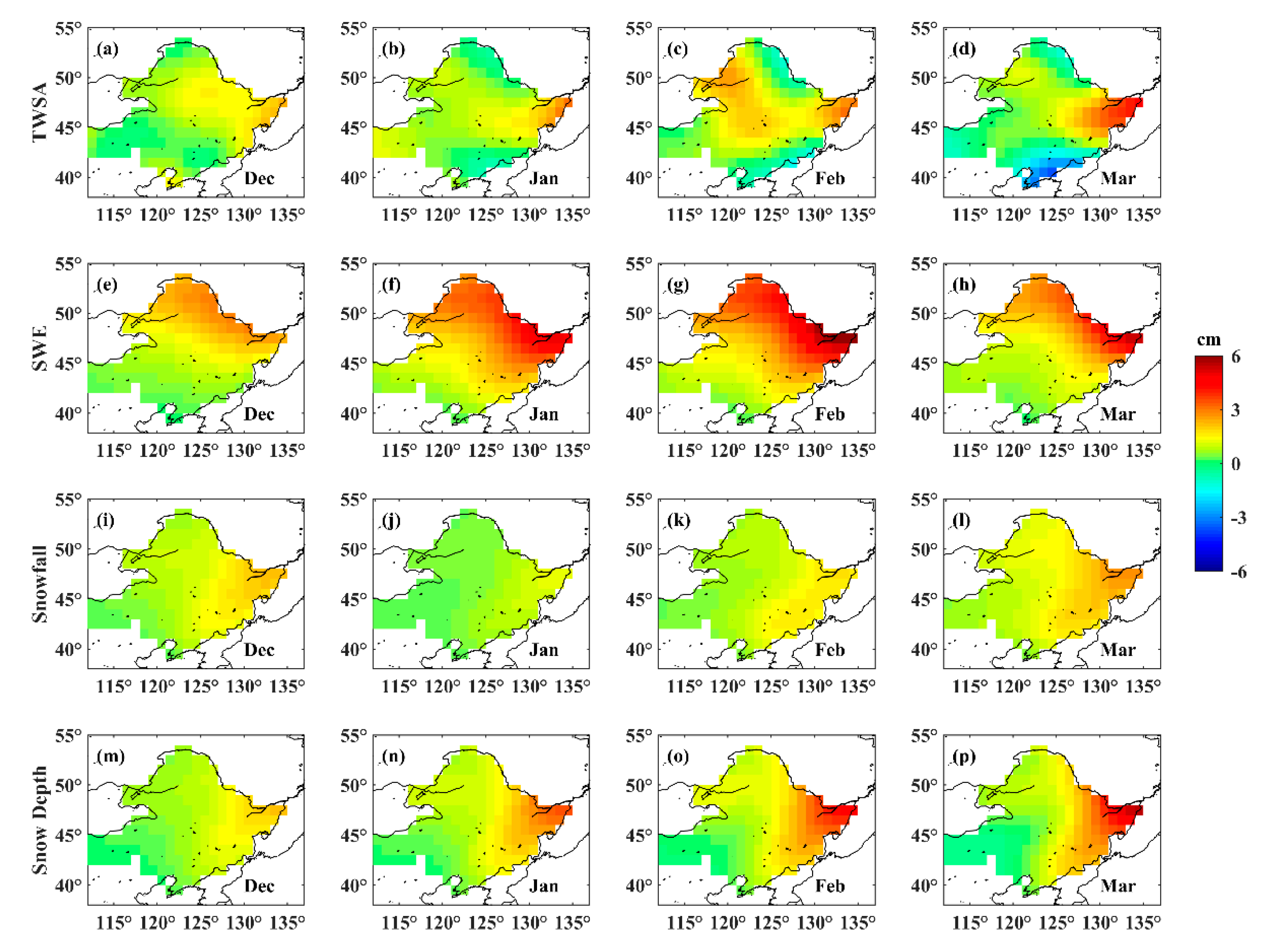
Figure 6 shows the spatial distribution of monthly variations of TWSA, SWE, snowfall, and snow depth in Northeast China. SWE, snow depth, and TWSA results were anomalies relative to their November values. The spatial distribution of snowfall and snow depth had a good consistency with their monthly mean variation series, as shown in Figure 5a, which confirmed the results discussed above. Snowfall in the Northeast China was greater in December and March than in January and February, with a gradual increase from January to March. Under the conditions of reduced evaporation and runoff activities in winter, snowfall was preserved primarily in the form of snow cover, resulting in increased snow depth from December to February. The spatial distributions of snowfall and snow depth in March were inconsistent, which was likely due to the impact of temperature on snow melt. However, SWE and snowfall as well as snow depth showed different spatial patterns. The GlobSnow SWE record is assimilated from space-borne passive radiometer data (SMMR, SSM/I, and SSMIS) and ground-based synoptic weather stations data, and thus it probably has large uncertainties affected by vegetation cover, topography impacts, and temperature [40]; therefore, the November SWE result may have been underestimated (Figure 5a). Consequently, when subtracting the November values from the SWE results, it will lead to higher values compared to snow depth, which was the main reason for the wide difference in the spatial patterns of snowfall, snow depth, and SWE.
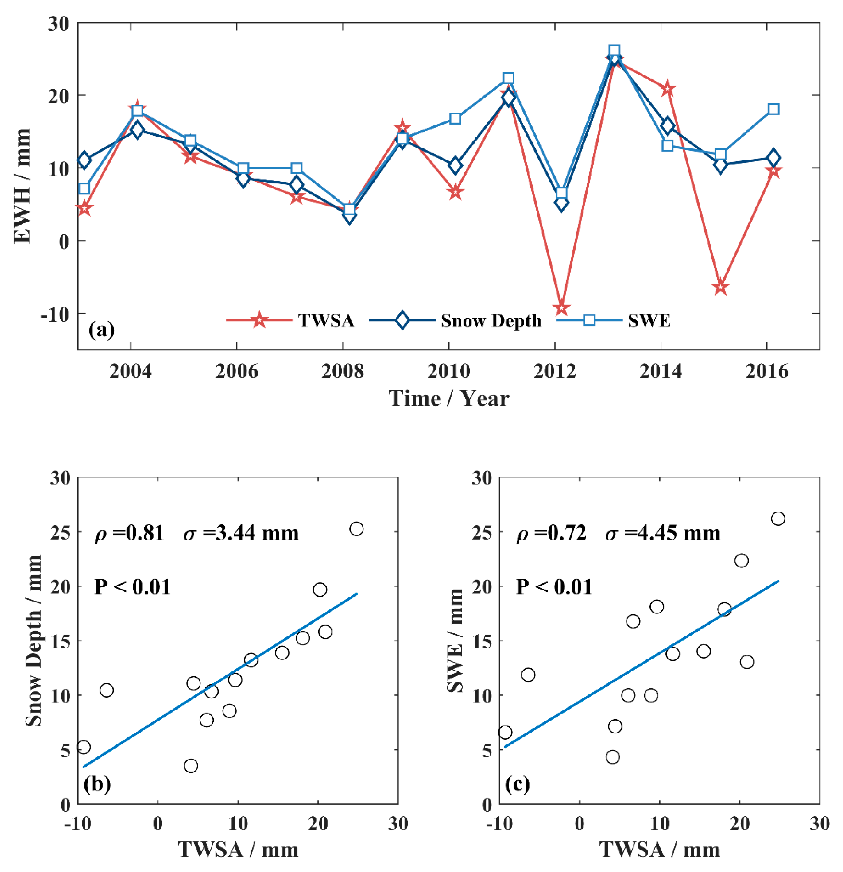
On the basis of the spatial distribution of the average monthly change of snowfall (Figure 6) and the average monthly series (Figure 5), we can see that snow cover of Northeast China generally reached its maximum in February. Winter precipitation of Northeast China occurred mainly in the form of snowfall, which dominated the TWS in Northeast China in winter. To quantify the effect of snowfall on TWS and verify the reliability of the GRACE data for detecting snow cover, we used the linear regression method to analyze the series of snow depth and water storage in February, when the snow storage reached the maximum. As shown in Figure 7, snow depth and TWSA in February were closely correlated. The correlation between snow depth and GRACE water storage reached 0.81, and the correlation between SWE and GRACE water storage reached 0.72, which can be regarded as a strong correlation [62]. The standard deviations of their differences were both less than 4.5mm, with a 99% confidence level.
In summary, rainfall and snowfall controlled the seasonal TWS changes of Northeast China in different seasons. There were two peaks in the seasonal variation of TWSA, being found in February and August. The winter TWSA peak in February was caused by snowfall, and the summer TWSA peak in August was controlled by rainfall. Although the seasonal amplitude of snowfall was only 1/10 that of rainfall, it had a much greater impact on the seasonal-scale TWSA, and summer rainfall brought about only a sub-peak with a 1-month delay. Furthermore, the annual amplitude and annual phase of snowfall and snow cover were generally consistent with winter TWSA calculated by GRACE. The time series of snow cover in February and TWSA calculated by GRACE were highly consistent, verifying that GRACE is a feasible means to monitor large-scale seasonal stable snow cover in Northeast China.
3.2. Impact of ENSO on Rainfall and TWSA in Northeast China
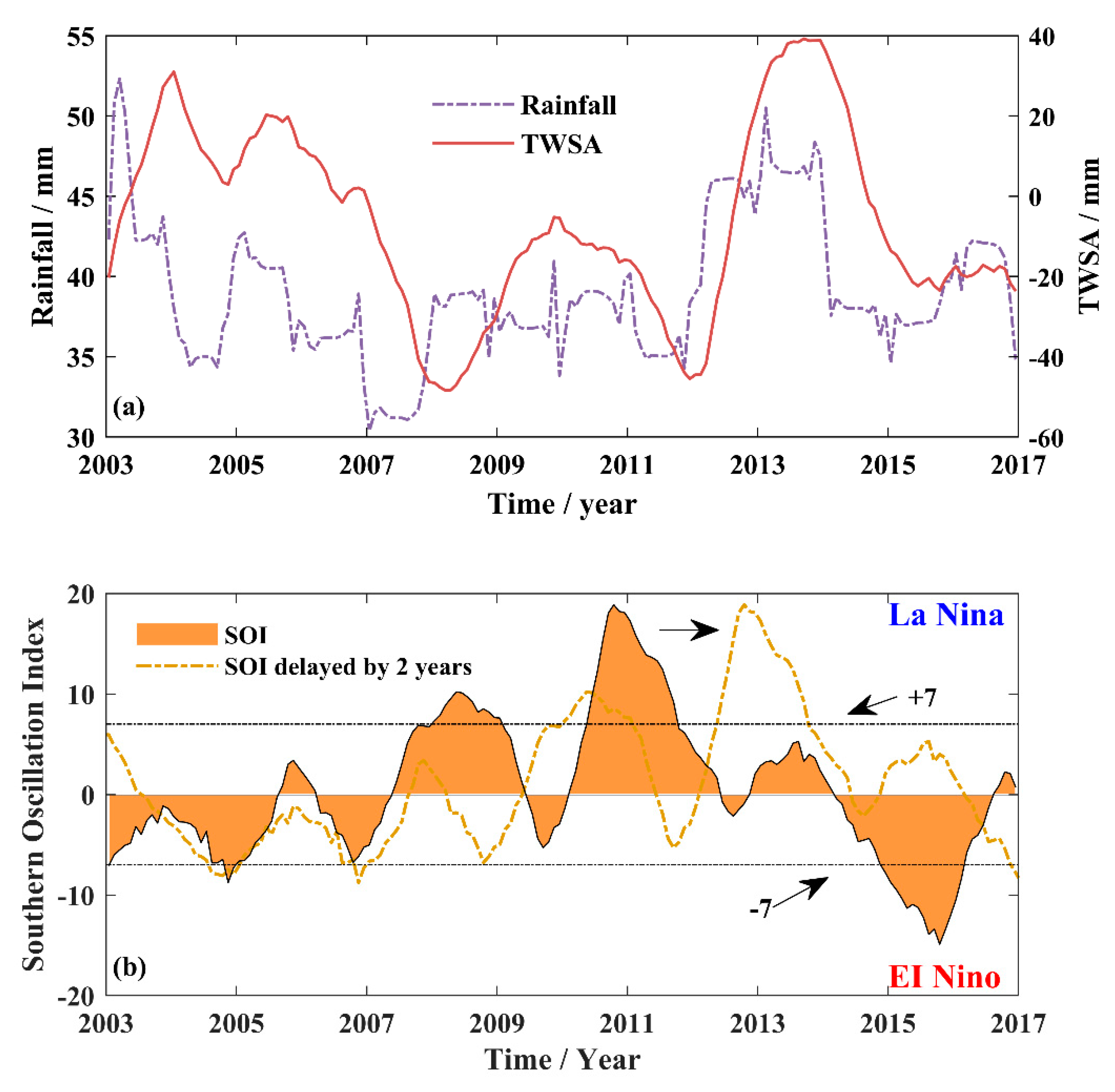
ENSO is an important factor for short-term climate predictions [63]. In China, ENSO events have a clear modulation effect on climate anomalies [32]. Here, we studied the response of TWS and rainfall to the ENSO phenomenon on an interannual scale in Northeast China. The interannual variation time series of TWSA, rainfall, and SOI are shown in Figure 8. When the time series of SOI was shifted back 2 years, we could tentatively conclude that the shifted SOI time series had an improved consistency with rainfall and TWSA series, as shown in Figure 8a. This preliminarily indicated that rainfall and water storage in Northeast China are influenced by the ENSO phenomenon, but that there is a lag of about 2 years.
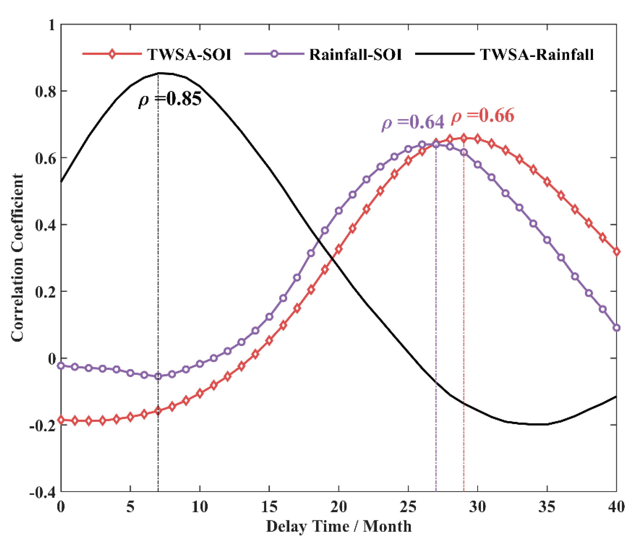
There were three strong ENSO events worldwide between 2003 and 2016: La Niña events in 2007–2008 and 2010–2011, and an El Niño event in 2015–2016. To analyze how the rainfall and TWSA in Northeast China were affected by these strong ENSO events, we selected a time lag range of 0–40 months to analyze the correlations among the interannual time series of SOI, TWSA, and rainfall from 2007 to 2016. As shown in Figure 9, the maximum correlation coefficient between TWSA and SOI in Northeast China was found to be 0.66, and the maximum correlation coefficient between rainfall and SOI was 0.64. TWSA and rainfall had a strong correlation with SOI, with lags of ≈29 months and ≈26 months behind SOI, respectively. In addition, the maximum value of the time series correlation coefficient between rainfall and interannual variation of TWSA was 0.85, with a lag of about 7 months. It has been shown that ENSO events modulate climate mainly by means of precipitation anomalies [64,65], which then modulate TWS [33]. The strong correlation among TWSA, rainfall, and SOI series indicates that the ENSO events influenced the interannual variation of rainfall and affected the interannual variation of TWS through rainfall. Lu et al. analyzed the relationship between drought (1949–1996) and ENSO events, and pointed out that the ENSO events may affect regional climate by influencing atmospheric circulation. They also have a significant impact on China’s precipitation and a lag of about 2 years in Northeast China [66], which is consistent with the findings presented in this paper. Thus, the impact of the ENSO events on precipitation and TWS in Northeast China is a long-term effect with a lag of about 2–3 years.
3.3. Simulation of the Interannual Contribution of Rainfall to TWS in Northeast China
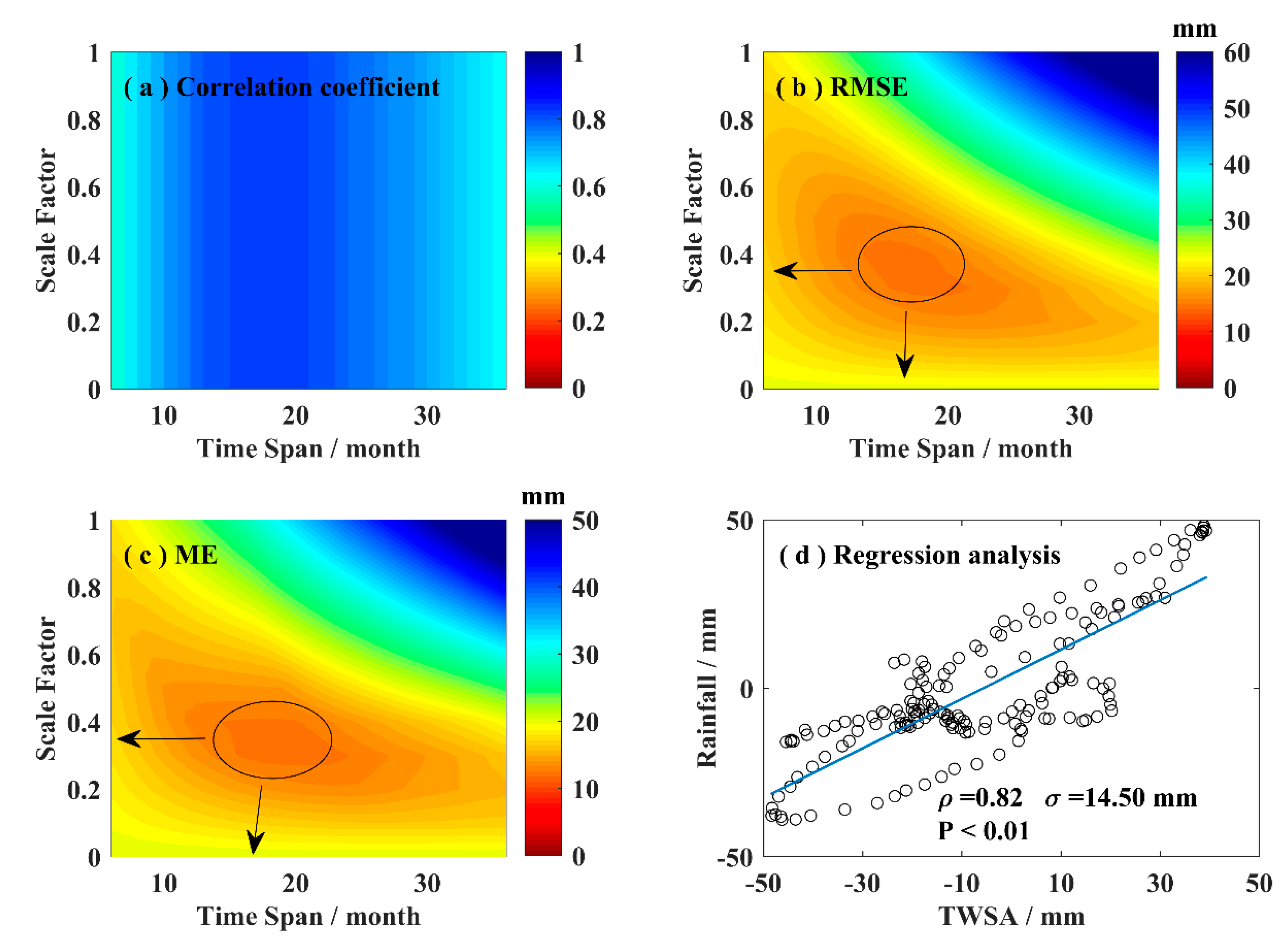
As mentioned in Section 3.2, the interannual variation of TWS is mainly influenced by rainfall in Northeast China. As shown in Figure 8a, the maximum interannual variations of TWSA and rainfall could reach 87.61 mm and 21.90 mm, respectively. However, the interannual variation of rainfall was found to only account for one-quarter of interannual variation of TWSA. This is mainly because there is a cumulative effect of rainfall on terrestrial water storage (i.e., rainfall in previous months still affects the variation of current water storage). Then, we constructed a model to simulate the contribution of rainfall to the interannual variation of TWSA (Equation (4)) [67]. In the model, n is the maximum number of months of cumulative rainfall, and a is the efficiency of the impact of rainfall. The model simulates the interannual variation time series of rainfall by continuously adjusting the values of n and a. The RMSE, mean error (ME) [61], and correlation coefficient between the simulation results and the water storage capacity were used as indicators of the evaluation accuracy. After continuous adjustment, the values of the parameters n and a were determined, and we obtained the simulation results of the effect of rain on the interannual variation of TWSA.
where a is the scale factor (0 < a < 1), t is the time (month) of simulated rainfall, Pi is the original rainfall value at the moment i, P0 is the mean rainfall value over the whole period, and f(t) is the TWSA at moment t.
n is taken as 6, 7, 8, …, 36, and a is taken as 0.1, 0.2, 0.3, …, 1.0. By continuously adjusting the values of n and a, the sequence of RMSE, ME, and correlation coefficients could finally be obtained, as shown in Figure 10a–c. It is shown that the correlation coefficient reached its maximum value (0.82) when n was 16, and the RMSE and ME reached their minimum values (14.50 mm, 12.04 mm) when n was also 16 and a was around 0.4. These results indicate that the possible ranges for n and a were 14–18 months and 0.3–0.4, respectively. To further obtain more reasonable values of n and a, we calculated the RMSE, ME, and correlation coefficients when n = 14/15/16/17/18 and a = 0.3/0.4, as shown in Table 2. We can see that RMSE reached its minimum and the correlation coefficient reached its maximum when n = 16 and a = 0.4. Thus, the maximum impact period of rainfall on TWS was about 16 months, with a scale factor a = 0.4.
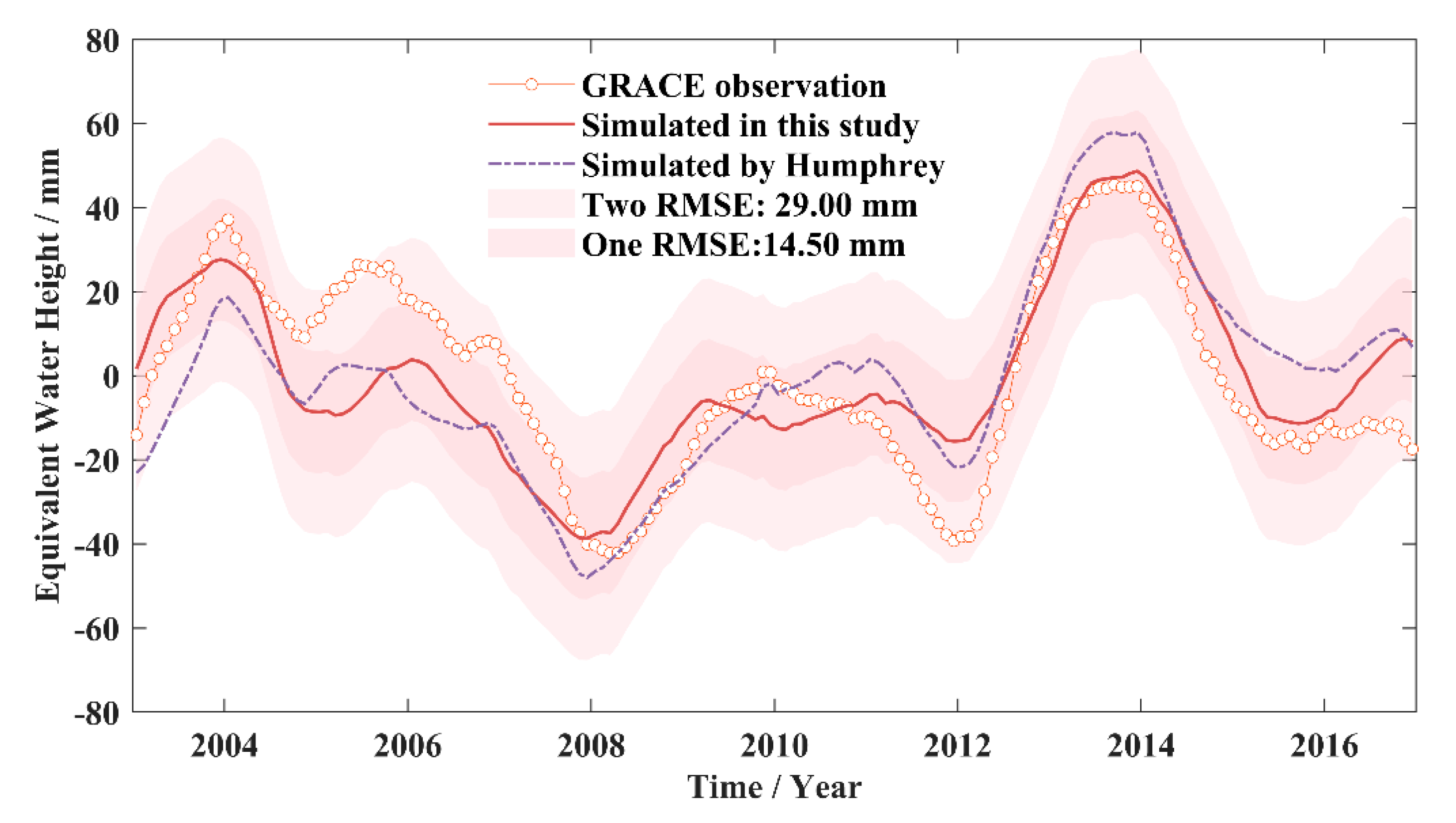
We used n = 16 and a = 0.4 to simulate the contribution of rainfall to the interannual TWSA from 2003 to 2016 (Figure 11). To be consistent with the simulated rainfall averages over the same timeframe, we implemented the GRACE results using a sliding average of 12 months. The RMSE value between GRACE and simulated result was 14.5 mm, and its RMSE difference was lower than 17% of the TWSA interannual variation, thus verifying the reliability of the model for the influence of rainfall on interannual land water storage changes in Northeast China given in this paper. In comparison, we calculated the simulation results of TWSA in Northeast China from 2003 to 2016 using data from the climate-driven water storage change model provided by Humphrey and Gudmundsson (2019) [68]. The results are shown in Figure 11, and all series were calculated on the basis of a 12-month sliding average. The model reconstructed by Humphrey and Gumundsson (GRACE-REC) showed a trend apparently larger than the long-term change of GRACE observations. We used a simpler reconstruction method than that of Humphrey and Gumundsson but yielded observations that were more consistent with GRACE.
4. Discussion
4.1. Challenge of Investigating Snow Cover Mass Change Using GRACE Data
In Northeast China, snowfall and snow cover account for a large proportion of TWS under conditions of reduced evaporation and runoff activity in winter. Therefore, we could use GRACE satellite data to detect seasonal large-scale variation of snow mass in Northeast China. Although GRACE satellite data has been used to assess the evolution of snow mass at high latitude [41,42], few studies have been conducted on snowfall in Northeast China. The result of this paper validated the ability of GRACE to monitor snow mass in a middle–high latitude region. As described in Section 3.1, the seasonal series of snowfall, snow depth, SWE, and TWSA presented good consistency. However, the mass signal detected by GRACE is a combination of all the mass variations, with signals from adjacent regions influencing each other [60]. As shown in Figure 6b–d, the negative signal in the northern region of Harbin may have been influenced by the spatial resolution constraints of the GRACE data and signal leakage. While there are various methods for correcting signal leakage errors, such as the spatial constraints method [30] and the scale factor method [69,70], these methods are mainly used to calculate the spatial distribution or rate of variation of TWS and groundwater storage. In contrast, this paper investigated the relationship between TWS and precipitation (snowfall and rainfall) mainly on seasonal and interannual scales. It did not calculate the trend terms, and thus the influence of signal leakage errors was not considered in this paper. Another limitation of this study was that we did not utilize the subsurface parameters (such as soil moisture and groundwater) from models. A previous study by Niu et al. [42] showed that SWE can be derived from TWS in arctic regions where subsurface observations can be accurately provided by hydrological models. However, Northeast China has a highly changeable water storage system (Figure 11), together with a mostly unknown groundwater network in a populated and agricultural region, making it hard to employ hydrological models for a reliable estimate. Furthermore, as mentioned in Section 3.1, there was a good consistency among the time seasonal series of TWSA, snowfall, and rainfall, while notable deviations still exist. For instance, the seasonal variation series of snow depth, SWE, and TWSA showed notable deviations in the years 2012 and 2015, as shown in Figure 7a. This might have been a result of the increase in missing data since 2011, leading to increased errors, as well as the extreme drought/wet events [48]. Thus, we discussed the ability of GRACE satellite data to monitor large-scale snow cover in a qualitative sense. In addition, constrained by the spatial resolution of GRACE, the TWSA shown here was only the result of regional average, without detailed spatially distributed features. It is difficult to investigate snow cover changes at a high spatial resolution only using GRACE data.
4.2. Uncertainties in ENSO Impact on Rainfall and TWS in Northeast China
As mentioned in Section 3.2, the impact of ENSO events on precipitation and TWS in Northeast China is a long-term effect with a lag of about 2–3 years. If we adjusted the time lag to 1–12 months, as shown in Figure 9, there was no significant correlation among the precipitation, TWSA, and SOI series. This is consistent with the results of Chen et al. (2020), who analyzed the impact of two strong ENSO events in 2005–2017 on regional TWS changes in China [32]. Thus, the impact of ENSO events on precipitation and water TWS in Northeast China has a feeble short-term effect.
In addition, when changing the period of correlation analysis, we obtained different results. As shown in Figure 12, we analyzed the correlations among the interannual time series of SOI, TWSA, and rainfall for 2003–2016, 2004–2016, 2005–2016, 2006–2016, and 2007–2016. This indicates that when different periods were used for analysis, the maximum correlation coefficient values and lag months among the interannual time series of TWSA, SOI, and rainfall were different. The interannual time series of TWSA and SOI did not show significant correlation in the periods of 2003–2016, 2004–2016, and 2005–2016, with correlation coefficients all being less than 0.4. Meanwhile, in the rest of the periods, TWSA and SOI interannual series showed a strong correlation, and the interannual time series of rainfall showed good consistence with SOI and TWSA. The poor correlation between TWSA and SOI series in the periods 2003–2016, 2004–2016, and 2005–2016 was mainly due to large-scale climate modes (i.e., Indian Ocean Dipole (IOD), North Atlantic Oscillation (NAO), and Pacific Decadal Oscillation (PDO)), which affect TWS in Northeast China, and was also limited by errors in the GRACE data [32,71]. Although different periods were chosen for the analysis, the conclusions were generally consistent. The TWSA and rainfall interannual time series lagged the SOI by ≈26 and ≈29 months, respectively, while the rainfall series lagged the TWSA by about 7 months. As mentioned above, there were three strong ENSO events worldwide in the period 2003–2016, and there was a strong correlation between TWSA and SOI series when strong ENSO events predominated in a given period. It can be confirmed that GRACE is only able to effectively monitor the impact of strong ENSO events on TWS in Northeast China.
5. Conclusions
In this study, we investigated the seasonal variation of rainfall and snowfall, the seasonal influence of rainfall on TWS, and the relationships between rainfall and TWS and ENSO phenomena in Northeast China on the basis of GRACE data, GlobSnow SWE products, ERA5-land monthly mean total precipitation, snowfall and snow depth data. We simulated the contribution of precipitation to terrestrial water storage in Northeast China from 2003 to 2016 and arrived at the following conclusions.
(1) The annual amplitude and phase of snowfall, snow cover, and TWSA in Northeast China were found to be generally consistent, reaching a maximum annual amplitude of about 6–12 mm around January. The annual amplitude of rainfall was about eight times that of snowfall and TWSA, but rainfall only had a moderate effect on the seasonal TWSA. Rainfall and snowfall controlled the seasonal variation of TWSA in Northeast China in different seasons. There were two peaks in the annual TWSA in Northeast China, with the winter peak mainly being caused by snowfall and the summer (usually August) peak being controlled by rainfall. Although the seasonal amplitude of snowfall was only 1/10 that of rainfall, it had a much greater impact on seasonal scale, while summer rainfall only brought about a sub-peak with a delay of 1 month.
(2) GRACE provided an effective means to monitor the stable seasonal snow cover over a large area. The annual amplitude and annual phase of TWSA calculated by GRACE were generally consistent with the results of snowfall and snow cover. At the 99% confidence level, the correlations between snow depth and SWE and TWSA series in February were 0.81 and 0.72, respectively. The results for the average monthly changes in the spatial distribution of rainfall, snowfall, snow depth, and TWSA from December to March also showed great consistency.
(3) TWS and rainfall in Northeast China were found to be affected by the ENSO phenomenon on the interannual scale. ENSO drove changes in TWS through precipitation, and then affected the interannual changes of TWS, which is a long-term effect with a lag of about 2–3 years. The correlation coefficient between rainfall and ENSO was 0.64, with a lag of about 26 months. The correlation coefficient between TWS and ENSO was 0.66, with a lag of about 29 months. The correlation coefficient between rainfall and TWSA was 0.85, with a lag of about 7 months.
(4) The effect of rainfall on TWS was the cumulative effect of rainfall. We constructed a model to estimate the contribution of rainfall to the interannual variation of TWS from 2003 to 2016 on the basis of TWS and rainfall data from the period 2003–2016.
Author Contributions
Conceptualization, methodology, validation, formal analysis, data curation, A.Q. and S.Y.; data curation, A.Q., S.Y., and L.C.; visualization, writing—original draft preparation, A.Q. and S.Y.; writing—review and editing, A.Q., S.Y., L.C., G.S., and X.L. All authors have read and agreed to the published version of the manuscript.
Funding
This research was funded by the Self-Funded Project of Scientific Research and Development Plan of Langfang Science and Technology Bureau (2020013045), Fundamental Scientific Research Business Expense for Higher School of Central Government (2020013045), and the Hebei Key Laboratory of Earthquake Dynamics Open Fund (FZ202214).
Acknowledgments
We are grateful to CSR, JPL, and GFZ for providing the monthly Release 06 solutions from which the DDK4 filter method was used to process the GRACE coefficients. The snowfall, snow depth, and total precipitation data were provided by the Climate Data Store. The SWE data were provided by the Finnish Meteorological Institute. We appreciate the editor and anonymous reviewers for their comments on the paper.
Conflicts of Interest
The authors declare no conflict of interest.
References
- Zeng, N.; Yoon, J.; Mariotti, A.; Swenson, S. Variability of Basin-Scale Terrestrial Water Storage from a PER Water Budget Method: The Amazon and the Mississippi. J. Clim. 2008, 21, 248–265. [Google Scholar] [CrossRef]
- Famiglietti, J.S. Remote sensing of terrestrial water storage, soil moisture and surface waters. Geophys. Monogr. 2004, 150, 197–207. [Google Scholar]
- Mo, X.; Wu, J.J.; Wang, Q.; Zhou, H. Variations in water storage in China over recent decades from GRACE observations and GLDAS. Nat. Hazards Earth Syst. Sci. 2016, 16, 469–482. [Google Scholar] [CrossRef] [Green Version]
- Li, B.; Rodell, M.; Zaitchik, B.F.; Reichle, R.H.; Koster, R.D.; Dam, T.M. Assimilation of GRACE terrestrial water storage into a land surface model: Evaluation and potential value for drought monitoring in western and central Europe. J. Hydrol. 2012, 446–447, 103–115. [Google Scholar] [CrossRef] [Green Version]
- Schmidt, R.; Schwintzer, P.; Flechtner, F.; Reigber, C.; Guentner, A.; Doell, P.; Ramillien, G.; Cazenave, A.; Petrovic, S.; Jochmann, H. GRACE observations of changes in continental water storage. Glob. Planet. Chang. 2006, 50, 112–126. [Google Scholar] [CrossRef]
- Rodell, M.; Houser, P.R.; Jambor, U.; Gottschalck, J.; Mitchell, K.; Meng, C.J.; Arsenault, K.; Cosgrove, B.; Radakovich, J.; Bosilovich, M.; et al. The Global Land Data Assimilation System. Bull. Am. Meteorol. Soc. 2004, 85, 381–394. [Google Scholar]
- Yin, W.; Li, T.; Zheng, W.; Hu, L.; Han, S.C.; Tangdamrongsub, N.; Šprlák, M.; Huang, Z. Improving regional groundwater storage estimates from grace and global hydrological models over Tasmania, Australia. Hydrogeol. J. 2020, 28, 1809–1825. [Google Scholar] [CrossRef]
- Ramillien, G.; Frappart, F.; Cazenave, A.; Güntnerb, A. Time variations of land water storage from an inversion of 2 years of GRACE geoids. Earth Planet. Sci. Lett. 2005, 235, 283–301. [Google Scholar] [CrossRef] [Green Version]
- Yin, W.; Hu, L.; Zhang, M.; Wang, J.; Han, S.C. Statistical Downscaling of GRACE-Derived Groundwater Storage Using ET Data in the North China Plain. J. Geophys. Res. Atmos. 2018, 123, 5973–5987. [Google Scholar] [CrossRef]
- Rodell, M.; Famiglietti, J.S. The potential for satellite-based monitoring of groundwater storage changes using GRACE: The High Plains aquifer, Central US. J. Hydrol. 2002, 263, 245–256. [Google Scholar] [CrossRef] [Green Version]
- Bi, H.; Ma, J.; Zheng, W.; Zeng, J. Comparison of soil moisture in gldas model simulations and in situ observations over the tibetan plateau. J. Geophys. Res. Atmos. 2016, 121, 2658–2678. [Google Scholar] [CrossRef] [Green Version]
- Wahr, J.; Molenaar, M.; Bryan, F. Time variability of the Earth’s gravity field: Hydrological and oceanic effects and their possible detection using GRACE. J. Geophys. Res. Solid Earth 1998, 103, 30205–30229. [Google Scholar] [CrossRef]
- Tapley, B.D.; Bettadpur, S.; Watkins, M.; Reigber, C. The gravity recovery and climate experiment: Mission overview and early results. Geophys. Res. Lett. 2004, 31, L09607. [Google Scholar] [CrossRef] [Green Version]
- Sun, W.K. Satellite in low orbit (CHAMP, GRACE, GOCE) and high precision earth gravity field. The latest progress of satellite gravity geodesy and its great influence on geoscience. J. Geod. Geodyn. 2002, 22, 92–100. [Google Scholar]
- Matsuo, K.; Heki, K. Coseismic gravity changes of the 2011 Tohoku-Oki earthquake from satellite gravimetry. Geophys. Res. Lett. 2011, 38, L00G12. [Google Scholar]
- Heki, K.; Matsuo, K. Coseismic gravity changes of the 2010 earthquake in central Chile from satellite gravimetry. Geophys. Res. Lett. 2010, 37, L24306. [Google Scholar] [CrossRef] [Green Version]
- Zemp, M.; Huss, M.; Thibert, E.; Eckert, N.; McNabb, R.; Huber, J.; Barandun, M.; Machguth, H.; Nussbaumer, S.; Gärtner-Roer, I. Global glacier mass changes and their contributions to sea-level rise from 1961 to 2016. Nature 2019, 568, 382–386. [Google Scholar] [CrossRef]
- Rignot, E.; Mouginot, J.; Scheuchl, B.; van den Broeke, M.; van Wessem, M.J.; Morlighem, M. Four decades of Antarctic ice sheet mass balance from 1979–2017. Proc. Natl. Acad. Sci. USA 2019, 116, 1095–1103. [Google Scholar] [CrossRef] [Green Version]
- Li, J.; Chen, J.; Ni, S.; Tang, L.; Hu, X. Long-term and inter-annual mass changes of Patagonia ice field from GRACE. Geod. Geodyn. 2019, 10, 100–109. [Google Scholar] [CrossRef]
- Yi, S.; Heki, K.; Qian, A. Acceleration in the global mean sea level rise: 2005–2015. Geophys. Res. Lett. 2017, 44, 11905–11913. [Google Scholar] [CrossRef] [Green Version]
- Chang, L.; Tang, H.; Yi, S.; Sun, W. The trend and seasonal change of sediment in the East China Sea detected by GRACE. Geophys. Res. Lett. 2019, 46, 1250–1258. [Google Scholar] [CrossRef]
- Ditmar, P. Conversion of time-varying stokes coefficients into mass anomalies at the earth’s surface considering the earth’s oblateness. J. Geod. 2018, 92, 1401–1412. [Google Scholar] [CrossRef] [PubMed] [Green Version]
- Ghobadi-Far, K.; Šprlák, M.; Han, S.C. Determination of Ellipsoidal Surface Mass Change from GRACE Time-Variable Gravity Data. Geophys. J. Int. 2019, 219, 248–259. [Google Scholar] [CrossRef]
- Feng, W.; Zhong, M.; Lemoine, J.; Richard, B.; Hsu, H.T.; Xia, J. Evaluation of groundwater depletion in North China using the Gravity Recovery and Climate Experiment (GRACE) data and ground-based measurements. Water Resour. Res. 2013, 49, 2110–2118. [Google Scholar] [CrossRef]
- Rodell, M.; Velicogna, I.; Famiglietti, J.S. Satellite-based estimates of groundwater depletion in India. Nature 2009, 460, 999–1002. [Google Scholar] [PubMed] [Green Version]
- Chen, J.L.; Wilson, C.R.; Tapley, B.D. The 2009 exceptional Amazon flood and interannual terrestrial water storage change observed by GRACE. Water Resour. Res. 2010, 46, W12526. [Google Scholar]
- Yang, Y.; E, D.-C.; Chao, D.-B.; Wang, H. Seasonal and inter-annual change in land water storage from GRACE. Chin. J. Geophys. 2009, 52, 2987–2992. [Google Scholar] [CrossRef]
- Forootan, E.; Schumacher, M.; Mehrnegar, N.; Bezděk, A.; Shum, C.K. An Iterative ICA-based Reconstruction Method to Produce Consistent Time-Variable Total Water Storage Fields using GRACE and Swarm Satellite Data. Remote Sens. 2020, 12, 1639. [Google Scholar]
- Feng, W.; Shum, C.; Zhong, M.; Pan, Y. Groundwater Storage Changes in China from Satellite Gravity: An Overview. Remote Sens. 2018, 10, 674. [Google Scholar] [CrossRef] [Green Version]
- Feng, W.; Wang, C.Q.; Mu, D.P.; Zhong, M.; Zhong, Y.L.; Xu, H.Z. Groundwater storage variations in the North China Plain from GRACE with spatial constraints. Chin. J. Geophys. 2017, 60, 1630–1642. [Google Scholar]
- Tangdamrongsub, N.; Han, S.C.; Jasinski, M.F.; Šprlák, M. Quantifying Water Storage Change and Land Subsidence Induced by Reservoir Impoundment Using GRACE, Landsat, and GPS Data. Remote Sens. Environ. 2019, 233, 111385. [Google Scholar] [CrossRef]
- Chen, W.; Zhong, M.; Feng, W.; Zhong, Y.L.; Xu, H.Z. Effects of two strong ENSO events on terrestrial water storage anomalies in China from GRRACE during 2005–2017. Chin. J. Geophys. 2020, 63, 141–154. (In Chinese) [Google Scholar]
- Zhang, Z.; Chao, B.F.; Chen, J.; Wilson, C.R. Terrestrial water storage anomalies of Yangtze River Basin droughts observed by GRACE and connections with ENSO. Glob. Planet. Chang. 2015, 126, 35–45. [Google Scholar] [CrossRef]
- Ni, S.; Chen, J.; Wilson, C.R.; Li, J.; Hu, X.; Fu, R. Global Terrestrial Water Storage Changes and Connections to ENSO Events. Surv. Geophys. 2018, 39, 1–22. [Google Scholar] [CrossRef]
- Zhong, Y.L.; Zhong, M.; Feng, W.; Zhang, Z.; Shen, Y.; Wu, D. Groundwater Depletion in the West Liaohe River Basin, China and Its Implications Revealed by GRACE and In Situ Measurements. Remote Sens. 2018, 10, 493. [Google Scholar]
- Hall, D.K.; Riggs, G.A.; Salomonson, V.V.; DiGirolamo, N.E.; Bayr, K.J. MODIS snow-cover products. Remote Sens. Environ. 2002, 83, 181–194. [Google Scholar] [CrossRef] [Green Version]
- Dong, J.; Walker, J.; Houser, P. Factors affecting remotely sensed snow water equivalent uncertainty. Remote Sens. Environ. 2005, 97, 68–82. [Google Scholar] [CrossRef]
- Su, H.; Yang, Z.L.; Niu, G.Y.; Dickinson, R.E. Enhancing the estimation of continental-scale snow water equivalent by assimilating modis snow cover with the ensemble kalman filter. J. Geophys. Res. Atmos. 2008, 113, D08120. [Google Scholar] [CrossRef] [Green Version]
- Nolin, A.W. Recent advances in remote sensing of seasonal snow. J. Glaciol. 2010, 56, 1141–1150. [Google Scholar] [CrossRef] [Green Version]
- Wang, S.; Zhou, F.; Russell, H.A.J. Estimating snow mass and peak river flows for the Mackenzie River basin using grace satellite observations. Remote Sens. 2017, 9, 256. [Google Scholar] [CrossRef] [Green Version]
- Frappart, F.; Ramillien, G.; Biancamaria, S.; Mognard, N.; Cazenave, A. Evolution of high-latitude snow mass derived from the grace gravimetry mission (2002–2004). Geophys. Res. Lett. 2006, 33, 356–360. [Google Scholar] [CrossRef] [Green Version]
- Niu, G.Y.; Seo, K.W.; Yang, Z.L.; Wilson, C.; Su, H.; Chen, J.; Rodell, M. Retrieving snow mass from grace terrestrial water storage change with a land surface model. Geophys. Res. Lett. 2007, 34, L15704. [Google Scholar] [CrossRef] [Green Version]
- Forman, B.A.; Reichle, R.H.; Rodell, M. Assimilation of terrestrial water storage from grace in a snow-dominated basin. Water Resour. Res. 2012, 48, W01507. [Google Scholar]
- Li, P.J.; Mi, D.S. Distribution of snow cover in China. J. Glaciol. Geocryol. 1983, 5, 9–18. [Google Scholar]
- Wang, C.H.; Wang, Z.L.; Cui, Y. Snow cover of China during the last 40 years: Spatial distribution and international variation. J. Glaciol. Geocryol. 2009, 31, 301–310. [Google Scholar]
- Zhong, Z.T.; Li, X.; Xu, X.C.; He, Z.Q. Spatial-temporal variations analysis of snow cover in China from 1992–2010. Chin. Sci. Bull. 2018, 63, 2641–2654. (In Chinese) [Google Scholar]
- Zhao, X.M.; Li, D.L.; Cheng, G.Y. GIS-based spatializing method for estimating snow cover depth in Northeast China and its nabes. Arid Zone Res. 2012, 29, 927–933. (In Chinese) [Google Scholar]
- Zheng, L.; Pan, Y.; Gong, H.; Huang, Z.; Zhang, C. Comparing Groundwater Storage Changes in Two Main Grain Producing Areas in China: Implications for Sustainable Agricultural Water Resources Management. Remote Sens. 2020, 12, 2151. [Google Scholar] [CrossRef]
- Cheng, M.; Ries, J.C.; Tapley, B.D. Variations of the earth’s figure axis from satellite laser ranging and GRACE. J. Geophys. Res. Solid Earth 2011, 116, B01409. [Google Scholar] [CrossRef] [Green Version]
- Landerer, F. Monthly Estimates of Degree-1 (Geocenter) Gravity Coefficients, Generated from GRACE (04-2002-06/2017) and GRACE-FO (06/2018 Onward) RL06 Solutions, GRACE Technical Note 13, the GRACE Project, NASA Jet Propulsion Laboratory. 2019. Available online: https://podaac-tools.jpl.nasa.gov/drive/files/allData/grace/docs/TN-13_GEOC_CSR_RL06.txt (accessed on 1 November 2020).
- Sun, Y.; Riva, R.; Ditmar, P. Optimizing estimates of annual variations and trends in geocenter motion and J2 from a combination of GRACE data and geophysical models. J. Geophys. Res. Solid Earth 2016, 121, 8352–8370. [Google Scholar] [CrossRef] [Green Version]
- Geruo, A.; Wahr, J.; Zhong, S. Computations of the viscoelastic response of a 3-D compressible Earth to surface loading: An application to Glacial Isostatic Adjustment in Antarctica and Canada. Geophys. J. Int. 2013, 192, 557–572. [Google Scholar]
- Kusche, J.; Schmidt, R.; Petrovic, S.; Rietbroek, R. Decorrelated GRACE time-variable gravity solutions by GFZ, and their validation using a hydrological model. J. Geod. 2009, 83, 903–913. [Google Scholar] [CrossRef] [Green Version]
- Farrell, W.E. Deformation of the Earth by surface loads. Rev. Geophys. 1972, 10, 761–797. [Google Scholar] [CrossRef]
- Globsnow. Available online: www.globsnow.info (accessed on 10 November 2020).
- Chen, X.; Li, X.; Wang, G.; Zhao, K.; Zheng, X.; Jiang, T. Based on Snow Cover Survey Data of Accuracy Veri-fication and Analysis of Passive Microwave Snow Cover Remote Sensing Products in Northeast China. Remote Sens. Technol. Appl. 2019, 34, 1181–1189. [Google Scholar]
- ERA5-European Environment Agency. Available online: https://www.eea.europa.eu/data-and-maps/data/external/era-interim-1 (accessed on 10 November 2020).
- Muñoz Sabater, J. ERA5-Land Monthly Averaged Data from 1981 to Present. Copernicus Climate Change Service (C3S) Climate Data Store (CDS). 2019. Available online: https://cds.climate.copernicus.eu/cdsapp#!/dataset/reanalysis-era5-land-monthly-means?tab=overview (accessed on 10 November 2020). [CrossRef]
- Climate Glossary-Southern Oscillation Index (SOI). Available online: http://www.bom.gov.au/climate/glossary/soi.shtml (accessed on 10 November 2020).
- Chang, L.; Sun, W. Greening Trends of Southern China Confirmed by GRACE. Remote Sens. 2020, 12, 328. [Google Scholar] [CrossRef] [Green Version]
- Zhang, S.B.; Wei, F.Y.; Liu, G.L.; Zhao, C.S.; Yu, X.X.; Zheng, C.Q.; Ning, Y.X.; Qian, J.G.; Shi, J.J. Celiang Pingcha, 1st ed.; China University of Mining and Technology Press: Xuzhou, China, 2008; pp. 7–132. (In Chinese) [Google Scholar]
- Cohen, J. Statistical Power Analysis. Curr. Dir. Psychol. Sci. 1992, 1, 98–101. [Google Scholar] [CrossRef]
- Santoso, A.; England, M.H.; Cai, W. Impact of Indo-Pacific Feedback Interactions on ENSO Dynamics Diagnosed Using Ensemble Climate Simulations. J. Clim. 2012, 25, 7743–7763. [Google Scholar]
- Zhou, L.T.; Wu, R. Respective impacts of the East Asian winter monsoon and ENSO on winter rainfall in China. J. Geophys. Res. 2010, 115, D02107. [Google Scholar] [CrossRef]
- Jiang, T.; Zhang, Q.; Zhu, D.; Wu, Y. Yangtze floods and droughts (China) and teleconnections with ENSO activities (1470–2003). Quat. Int. 2006, 144, 29–37. [Google Scholar]
- Lu, A.G.; Ge, J.P.; Pang, D.Q. Asynchronous Response of Droughts to ENSO in China. J. Glaciol. Geocryol. 2006, 28, 535–542. [Google Scholar]
- Yi, S.; Song, C.Q.; Heki, K.; Kang, S.; Chang, L. Satellite-observed monthly glacier and snow mass changes in southeast Tibet: Implication for substantial meltwater contribution to the Brahmaputra. Cryosphere 2020, 14, 2267–2281. [Google Scholar] [CrossRef]
- Humphrey, V.; Gudmundsson, L. GRACE-REC: A reconstruction of climate-driven water storage changes over the last century. Earth Syst. Sci. Data 2019, 11, 1153–1170. [Google Scholar] [CrossRef] [Green Version]
- Klees, R.; Zapreeva, E.A.; Winsemius, H.C.; Savenije, H.H.G. The bias in GRACE estimates of continental water storage variations. Hydrol. Earth Syst. Sci. 2007, 11, 1227–1241. [Google Scholar] [CrossRef] [Green Version]
- Longuevergne, L.; Scanlon, B.R.; Wilson, C.R. GRACE Hydrological estimates for small basins: Evaluating processing approaches on the High Plains Aquifer, USA. Water Resour. Res. 2010, 46, W11517. [Google Scholar] [CrossRef]
- Huang, Q.Z.; Zhang, Q.; Xu, C.Y.; Li, Q.; Sun, P. Terrestrial Water Storage in China: Spatiotemporal Pattern and Driving Factors. Sustainability 2019, 11, 6646. [Google Scholar] [CrossRef] [Green Version]
Figure 1.
Geographic setting of the research area.

Figure 2.
Time series of terrestrial water storage anomalies (TWSA) in Northeast China from 2003 to 2016 calculated on the basis of Gravity Recovery and Climate Experiment (GRACE) data: (a) time series of TWSA estimated using CSR (the Center for Space Research at the University of Texas at Austin), JPL (the Jet Propulsion Laboratory), and GFZ (the German Geosciences Research Center) solutions and their average; (b) interannual and seasonal signals of TWSA in Northeast China.

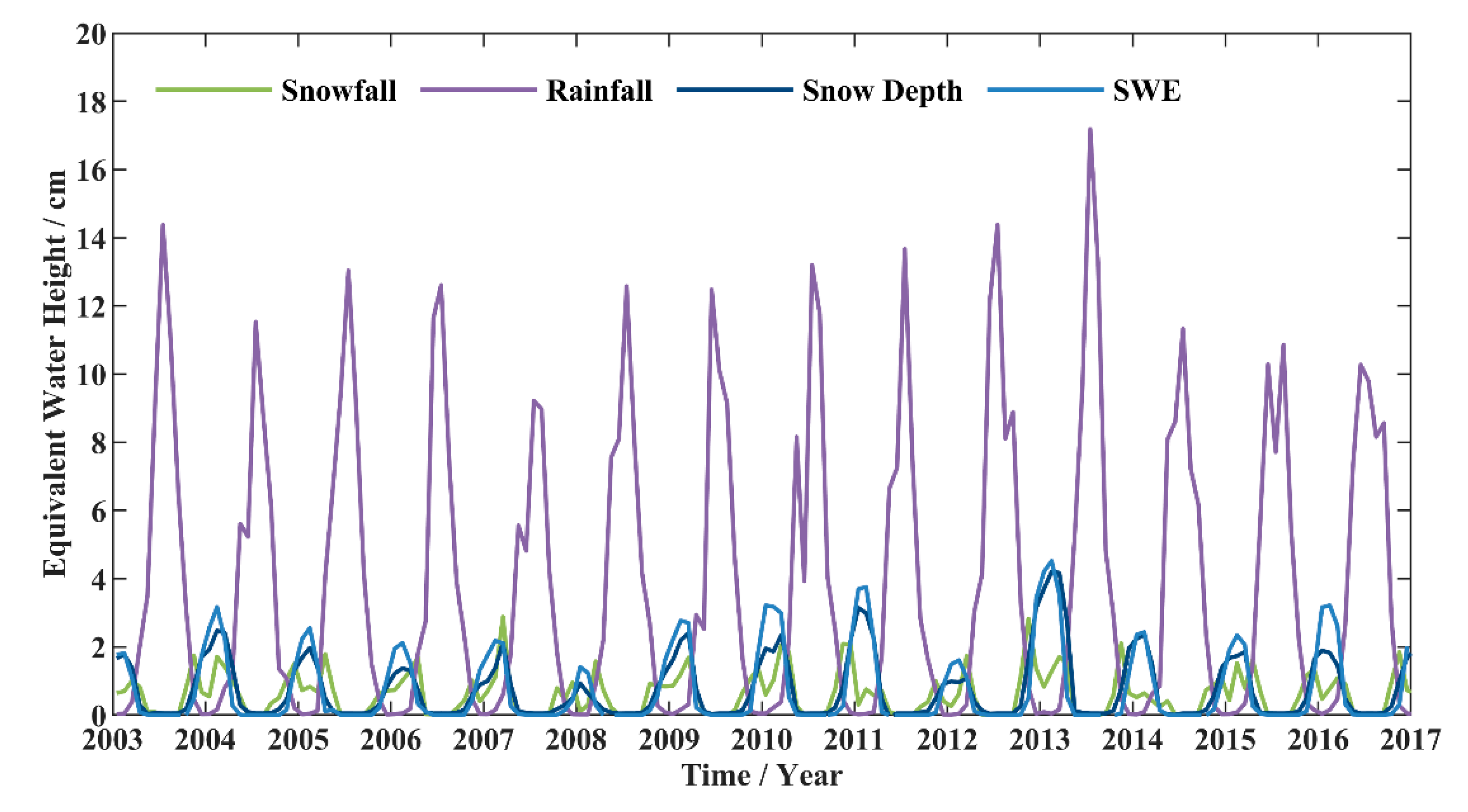
Figure 3.
Time series of rainfall, snowfall, and snow depth in Northeast China from 2003 to 2016.

Figure 4.
Time series and periodogram results of seasonal variation of TWSA, rainfall, snowfall, and snow depth in Northeast China: (a) time series of seasonal variation of TWSA, rainfall, snowfall, and snow depth in Northeast China; (b–f) periodogram results of TWSA, rainfall, snowfall, and snow depth in Northeast China.

Figure 5.
Monthly mean variation of rainfall, precipitation, and TWSA in Northeast China: (a) monthly mean variation of precipitation and TWSA in Northeast China; (b) monthly mean variation of rainfall in Northeast China.
Figure 5.
Monthly mean variation of rainfall, precipitation, and TWSA in Northeast China: (a) monthly mean variation of precipitation and TWSA in Northeast China; (b) monthly mean variation of rainfall in Northeast China.

Figure 6.
The spatial distribution of monthly variation of TWSA, snow water equivalent (SWE), snowfall, and snow depth in Northeast China (SWE, snow depth, and TWSA results were anomalies relative to their November values): (a–d) the spatial distribution of monthly variation of TWSA from December to March; (e–h) the spatial distribution of monthly variation of SWE from December to March; (i–l) the spatial distribution of monthly variation of snowfall from December to March; (m–p) the spatial distribution of monthly variation of snow depth from December to March.

Figure 7.
Time series and regression analysis results of seasonal variation of snow depth and TWSA in February: (a) time series of seasonal variation of snow depth and TWSA in February; (b) regression analysis results of seasonal variation of snow depth and TWSA in February; (c) regression analysis results of seasonal variation of SWE and TWSA in February.

Figure 8.
Annual variation series of precipitation, TWSA, and Southern Oscillation Index (SOI) in Northeast China: (a) annual variation series of precipitation and TWSA in Northeast China; (b) annual variation series of SOI in Northeast China.
Figure 8.
Annual variation series of precipitation, TWSA, and Southern Oscillation Index (SOI) in Northeast China: (a) annual variation series of precipitation and TWSA in Northeast China; (b) annual variation series of SOI in Northeast China.

Figure 9.
Correlations among the interannual time series of SOI, TWSA, and rainfall from 2007 to 2016. A time lag range of 0–40 months was selected to analyze the correlations among the interannual time series of SOI, TWSA, and rainfall from 2007 to 2016. TWSA-SOI represents the delayed correlation curve between TWSA and SOI interannual time series, Rainfall-SOI represents the delayed correlation curve between rainfall and SOI interannual time series, and TWSA-Rainfall represents the delayed correlation curve between TWSA and rainfall interannual time series.

Figure 10.
Root mean square errors (RMSE), mean error (ME), and correlation values and regression analysis results over different time spans: (a) correlation coefficient values over different time spans; (b) RMSE values over different time spans; (c) ME values over different time spans; (d) results of regression analysis of rainfall and TWSA series when n = 16 and a = 0.4.

Figure 11.
Simulation results of the contribution of precipitation to the annual variation of TWS.

Figure 12.
Results of correlation analysis over different periods: (a) correlation values among TWSA, rainfall, and SOI over different time spans; (b) time lags among TWSA, rainfall, and SOI over different time spans.
Figure 12.
Results of correlation analysis over different periods: (a) correlation values among TWSA, rainfall, and SOI over different time spans; (b) time lags among TWSA, rainfall, and SOI over different time spans.


Table 1.
Annual amplitude of seasonal variation of TWSA, rainfall, snowfall, and snow depth in Northeast China. Uncertainties are estimated through error propagation [61].
Table 1.
Annual amplitude of seasonal variation of TWSA, rainfall, snowfall, and snow depth in Northeast China. Uncertainties are estimated through error propagation [61].
| Data Style | Annual Amplitude/mm | σ/mm | Annual Phase/Month | σ/Month |
|---|---|---|---|---|
| TWSA | 6.64 | 2.16 | 0.94 (January) | 0.44 |
| Rainfall | 56.64 | 2.17 | 6.51 (June–July) | 0.05 |
| Snowfall | 5.81 | 0.64 | 0.79 (January) | 0.15 |
| Snow depth | 10.33 | 0.60 | 1.11 (January) | 0.08 |
| SWE | 12.40 | 0.65 | 1.08 (January) | 0.07 |
Table 2.
Partial accuracy index values.
| Number | n/Month | a | RMSE/mm | ME/mm | Correlation Coefficient |
|---|---|---|---|---|---|
| 1 | 14 | 0.3 | 15.54 | 13.06 | 0.81 |
| 2 | 14 | 0.4 | 14.82 | 12.52 | 0.81 |
| 3 | 15 | 0.3 | 15.16 | 12.66 | 0.82 |
| 4 | 15 | 0.4 | 14.59 | 12.44 | 0.82 |
| 5 | 16 | 0.3 | 14.86 | 12.35 | 0.82 |
| 6 | 16 | 0.4 | 14.50 | 12.37 | 0.82 |
| 7 | 17 | 0.3 | 14.67 | 12.14 | 0.82 |
| 8 | 17 | 0.4 | 15.53 | 12.34 | 0.82 |
| 9 | 18 | 0.3 | 14.57 | 12.04 | 0.82 |
| 10 | 18 | 0.4 | 14.72 | 12.32 | 0.82 |
Publisher′s Note: MDPI stays neutral with regard to jurisdictional claims in published maps and institutional affiliations. |
© 2020 by the authors. Licensee MDPI, Basel, Switzerland. This article is an open access article distributed under the terms and conditions of the Creative Commons Attribution (CC BY) license (http://creativecommons.org/licenses/by/4.0/).
Share and Cite
MDPI and ACS Style
Qian, A.; Yi, S.; Chang, L.; Sun, G.; Liu, X. Using GRACE Data to Study the Impact of Snow and Rainfall on Terrestrial Water Storage in Northeast China. Remote Sens. 2020, 12, 4166. https://0-doi-org.brum.beds.ac.uk/10.3390/rs12244166
AMA Style
Qian A, Yi S, Chang L, Sun G, Liu X. Using GRACE Data to Study the Impact of Snow and Rainfall on Terrestrial Water Storage in Northeast China. Remote Sensing. 2020; 12(24):4166. https://0-doi-org.brum.beds.ac.uk/10.3390/rs12244166
Chicago/Turabian StyleQian, An, Shuang Yi, Le Chang, Guangtong Sun, and Xiaoyang Liu. 2020. "Using GRACE Data to Study the Impact of Snow and Rainfall on Terrestrial Water Storage in Northeast China" Remote Sensing 12, no. 24: 4166. https://0-doi-org.brum.beds.ac.uk/10.3390/rs12244166
Note that from the first issue of 2016, this journal uses article numbers instead of page numbers. See further details here.