Spatio-Temporal Characteristics of Drought Events and Their Effects on Vegetation: A Case Study in Southern Tibet, China

 , and
, and
Abstract
:
1. Introduction
2. Materials and Methods
2.1. Data Sources
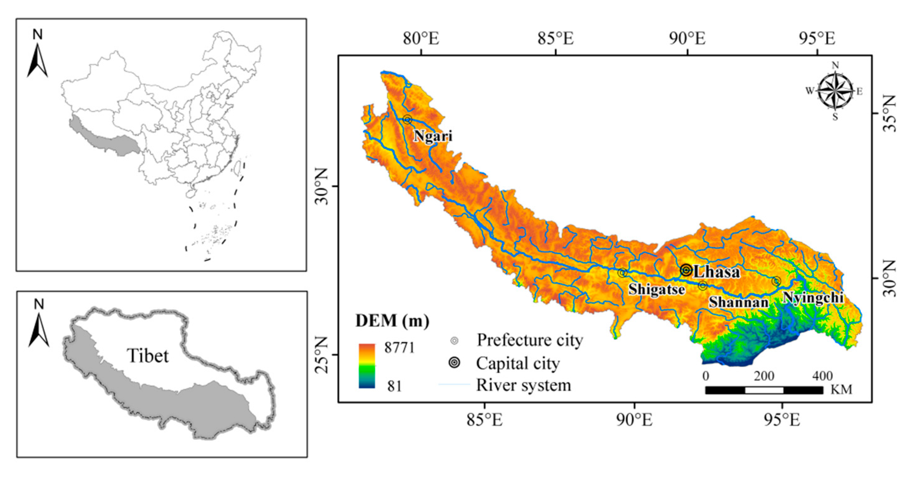
2.1.1. Study Area
2.1.2. Meteorological Data
2.1.3. Global Inventory Modelling and Mapping Studies (GIMMS) NDVI
2.1.4. Topographic Parameters
2.1.5. Soil Texture
2.1.6. Vegetation Type
2.2. Methodology
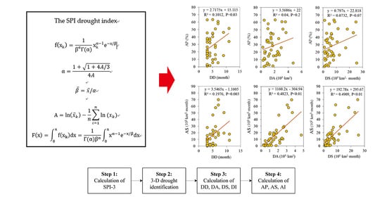
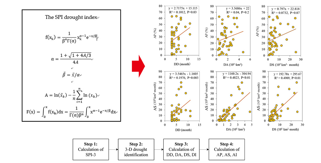
2.2.1. Calculation of the SPI
2.2.2. Drought Identification
2.2.3. Drought Characteristics
2.2.4. Vegetation Anomaly Index
2.2.5. Vegetation Characteristics under Drought Stress
2.2.6. Multivariate Linear Regression (MLR)
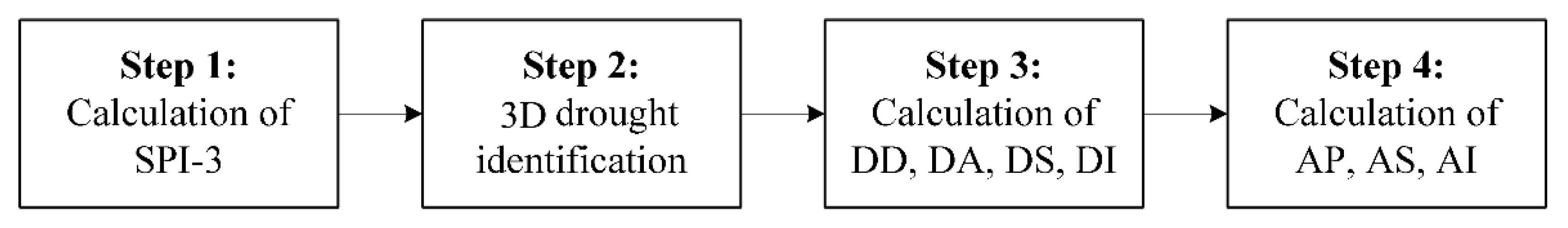
2.2.7. The Overall Flowchart of the Methodology
3. Result
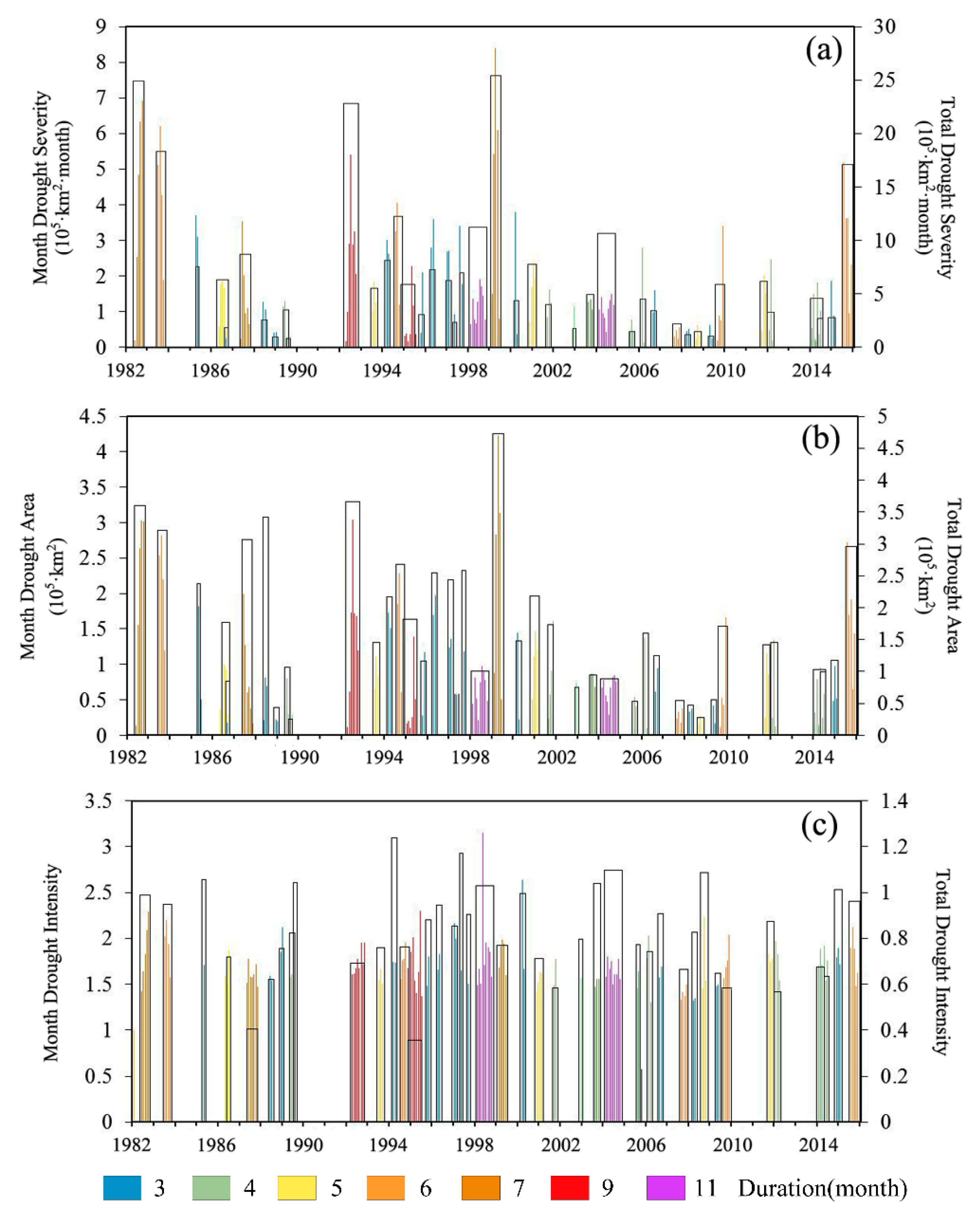
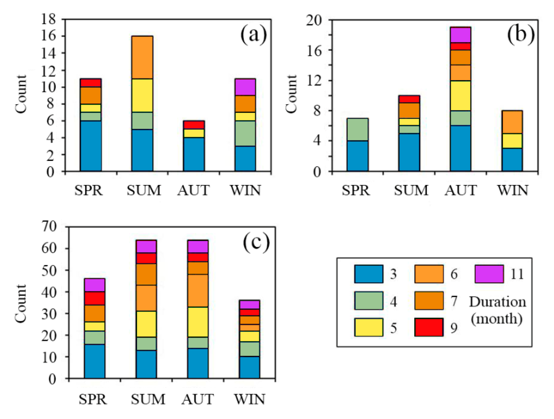
3.1. Temporal Characteristics of Drought Events
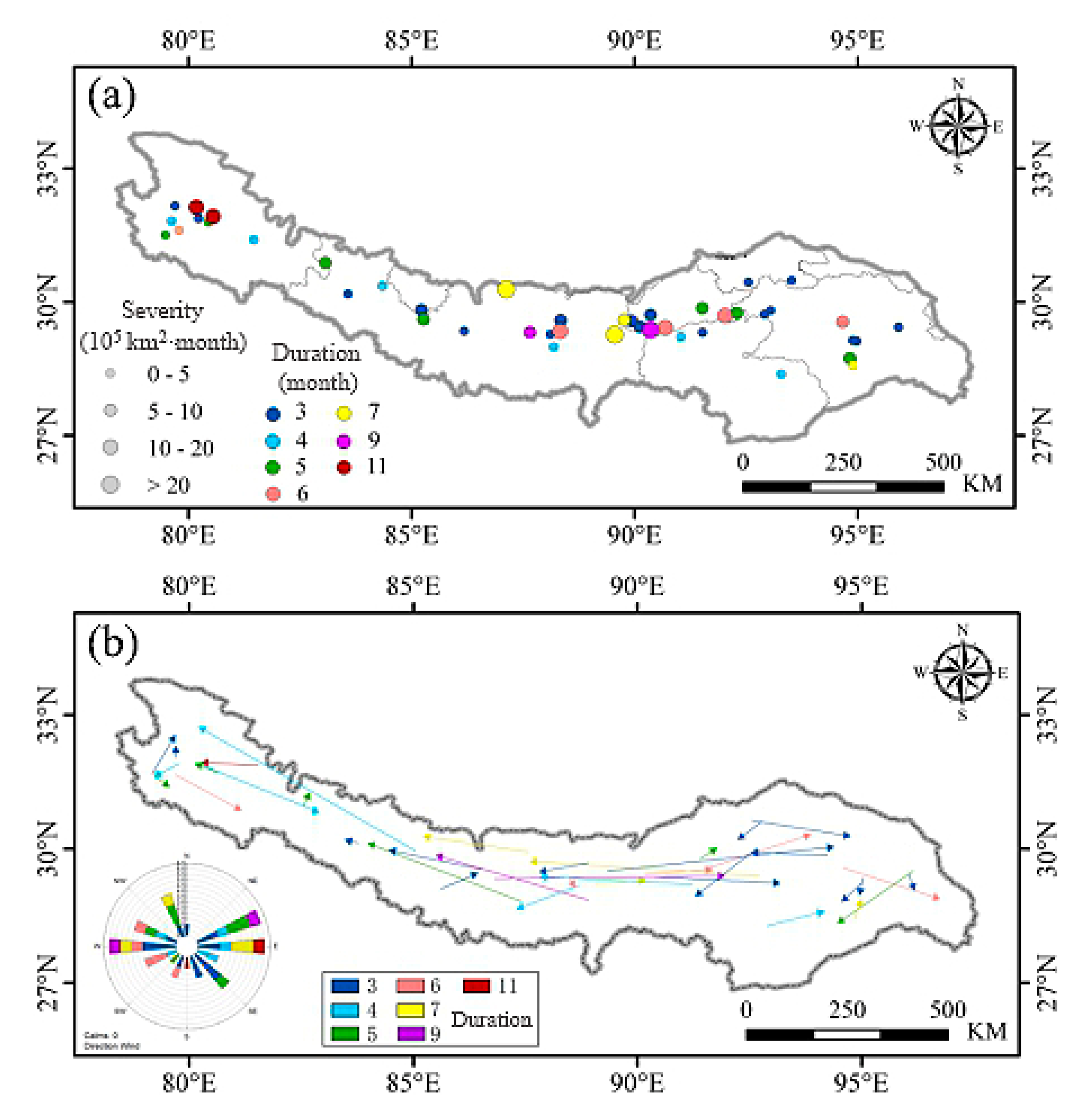
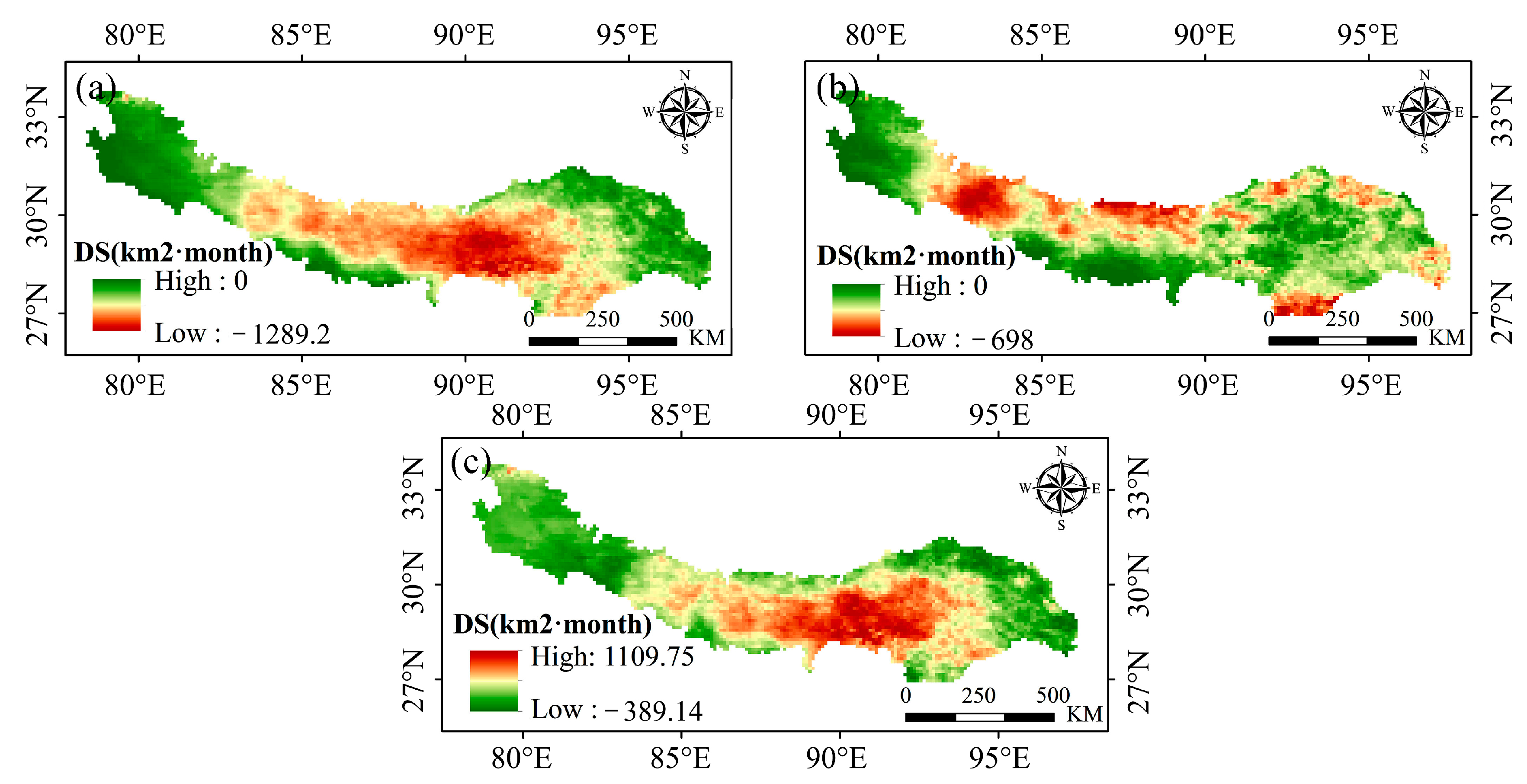
3.2. Spatial Characteristics of Drought Events
3.3. Evaluation of a Single Drought Event
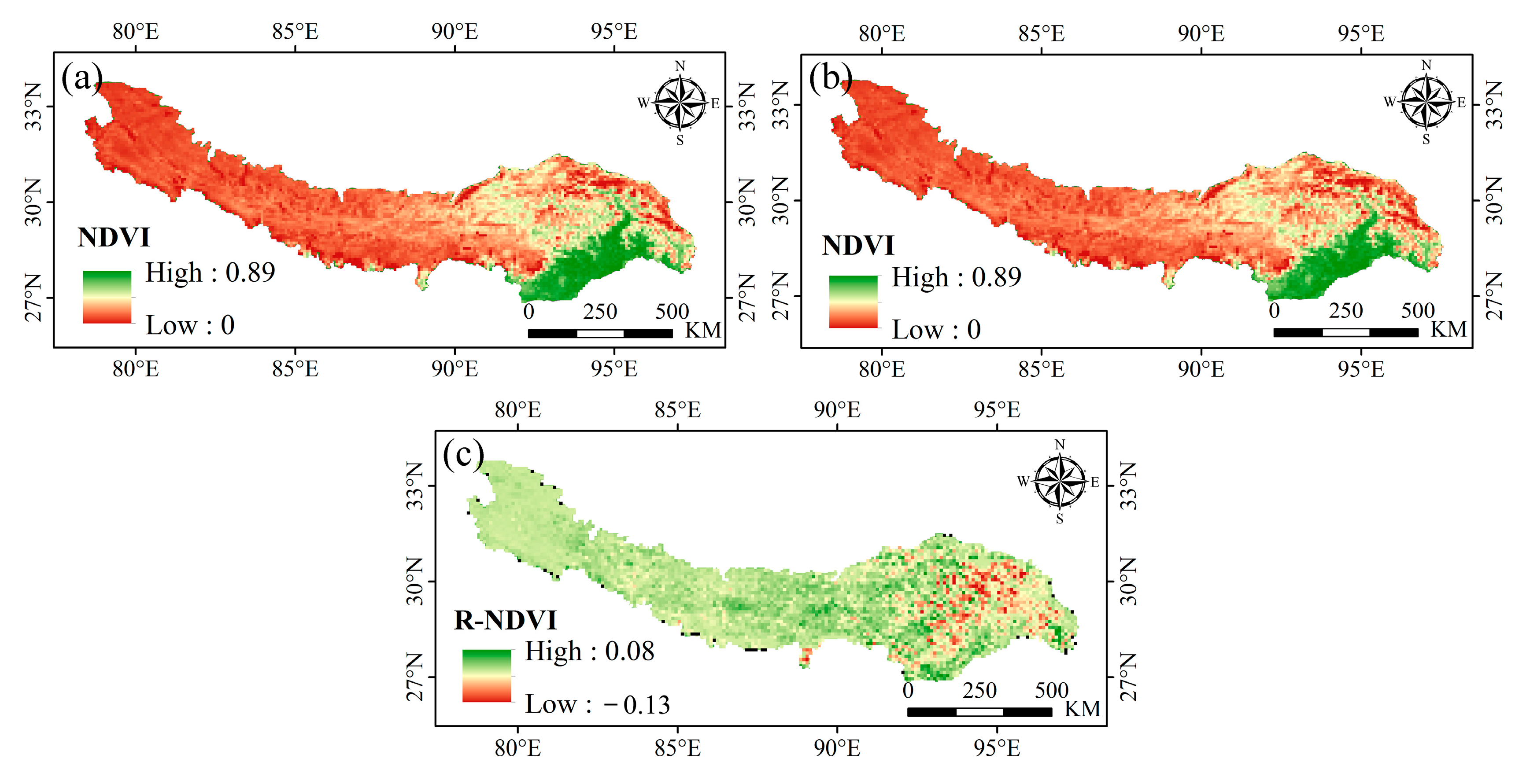
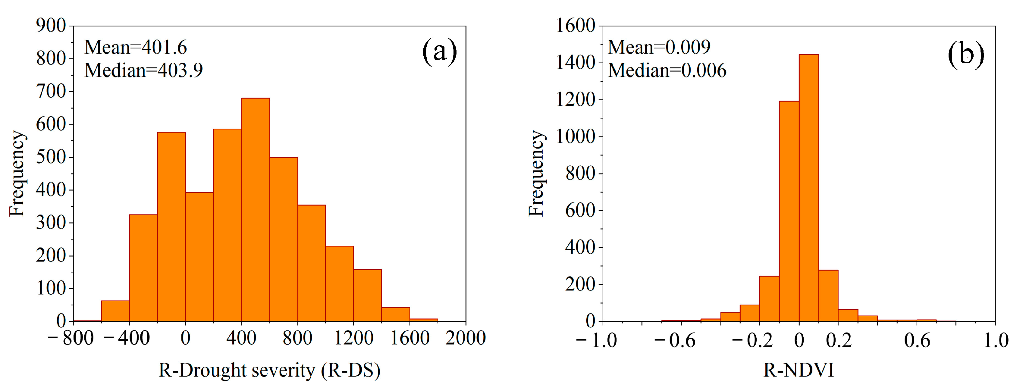
3.3.1. Effects of a Single Drought Event on Vegetation
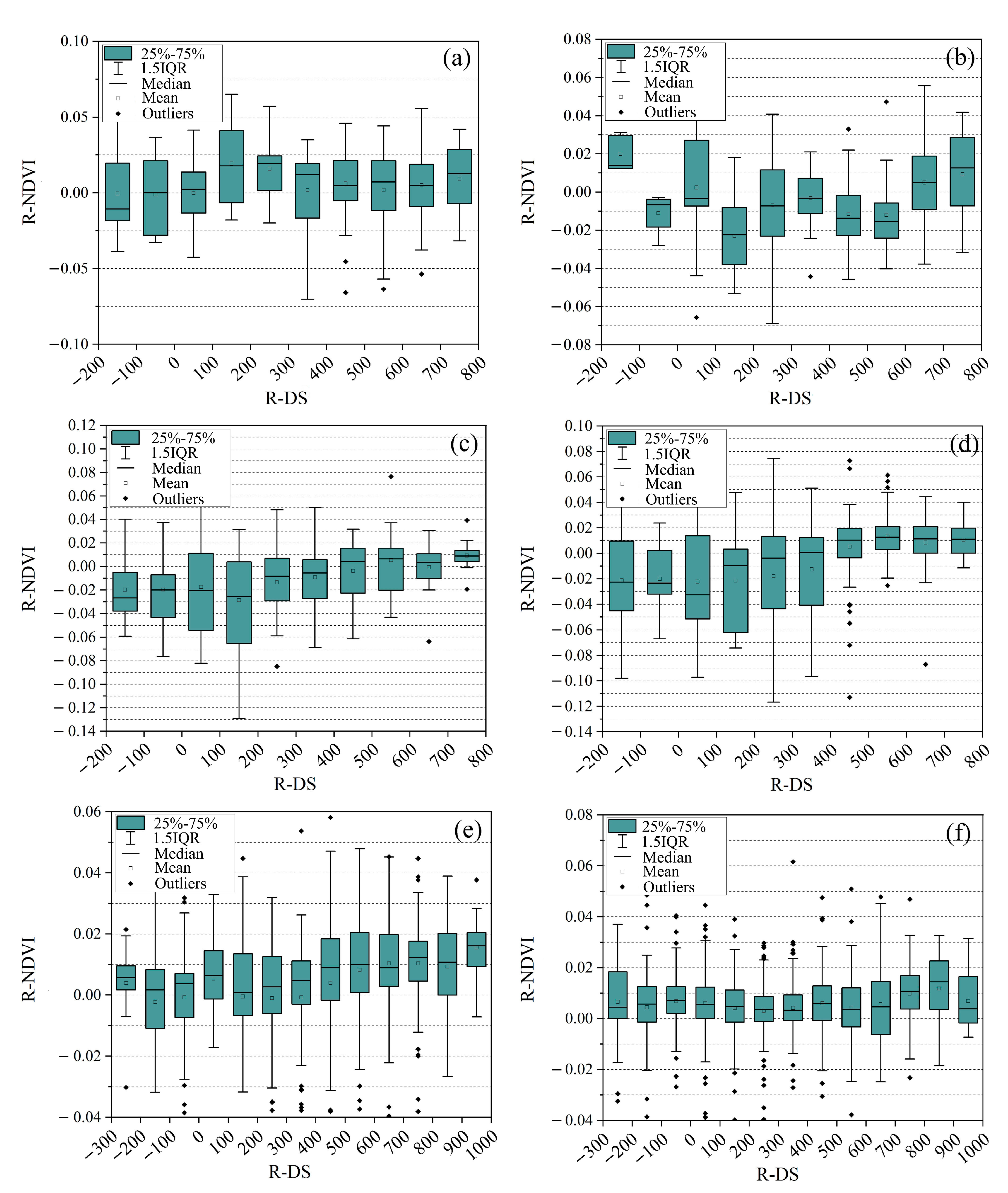
3.3.2. Different Responses of Vegetation Types and Elevation Bands
3.4. Assessment of the Effects of Multiple Drought Events Effects on Vegetation
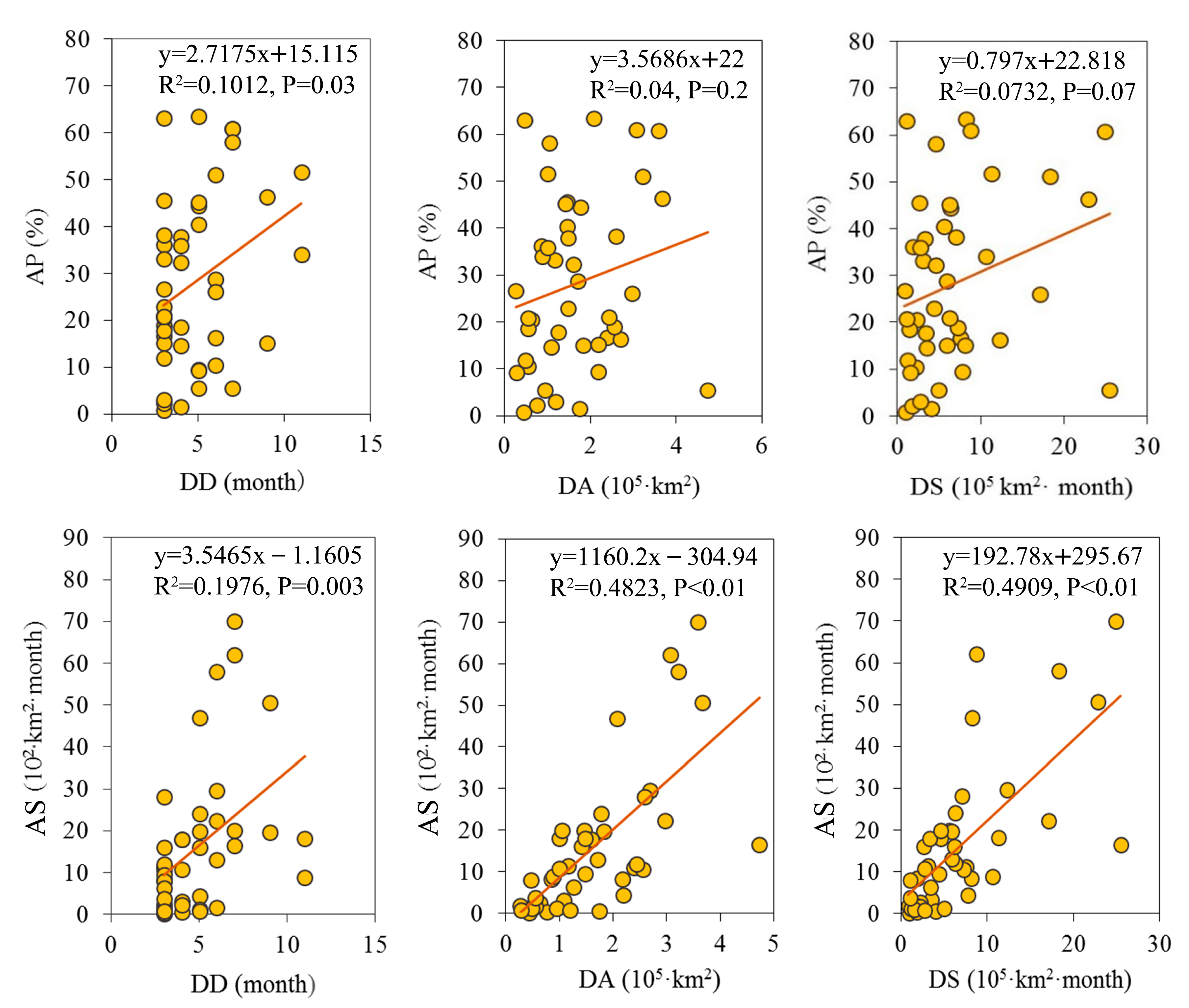
3.4.1. Relationships between Drought and Vegetation Characteristics
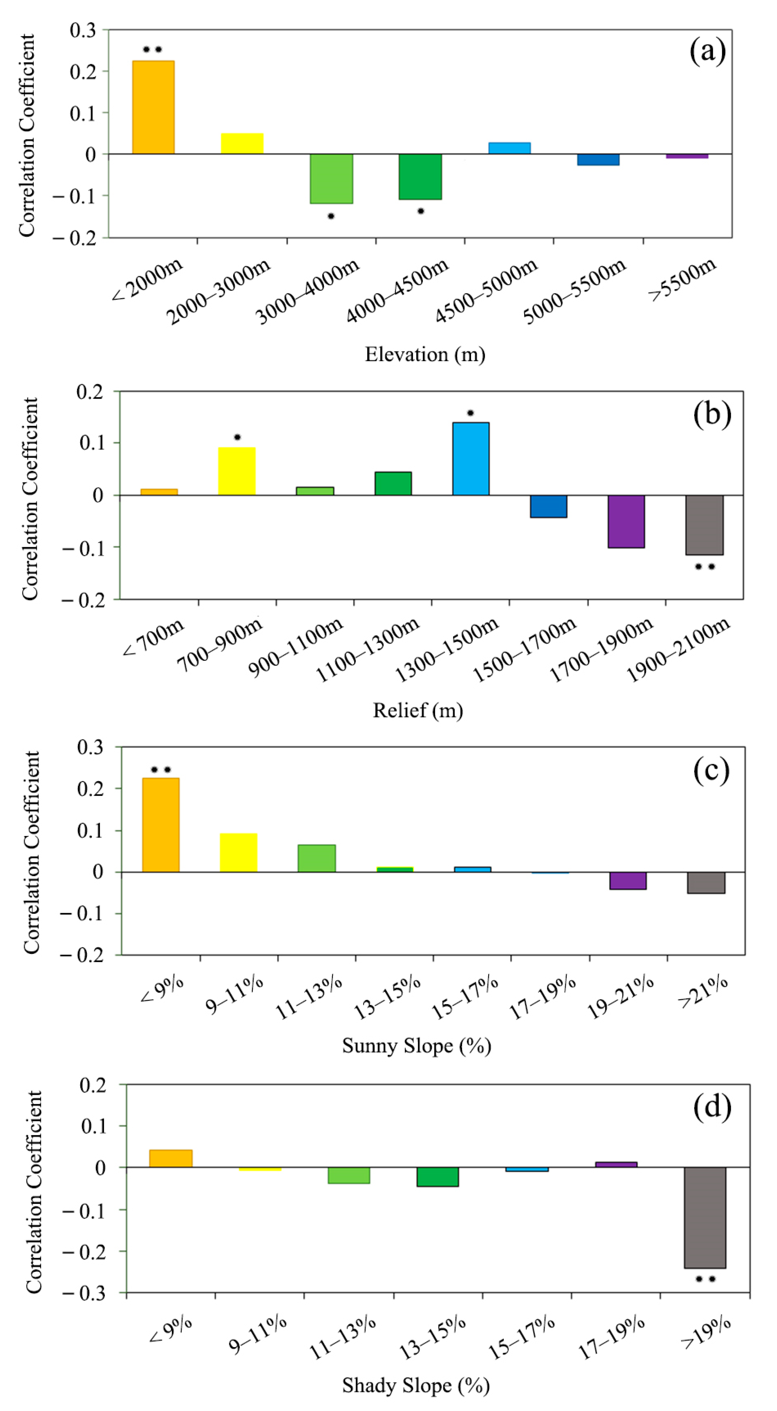
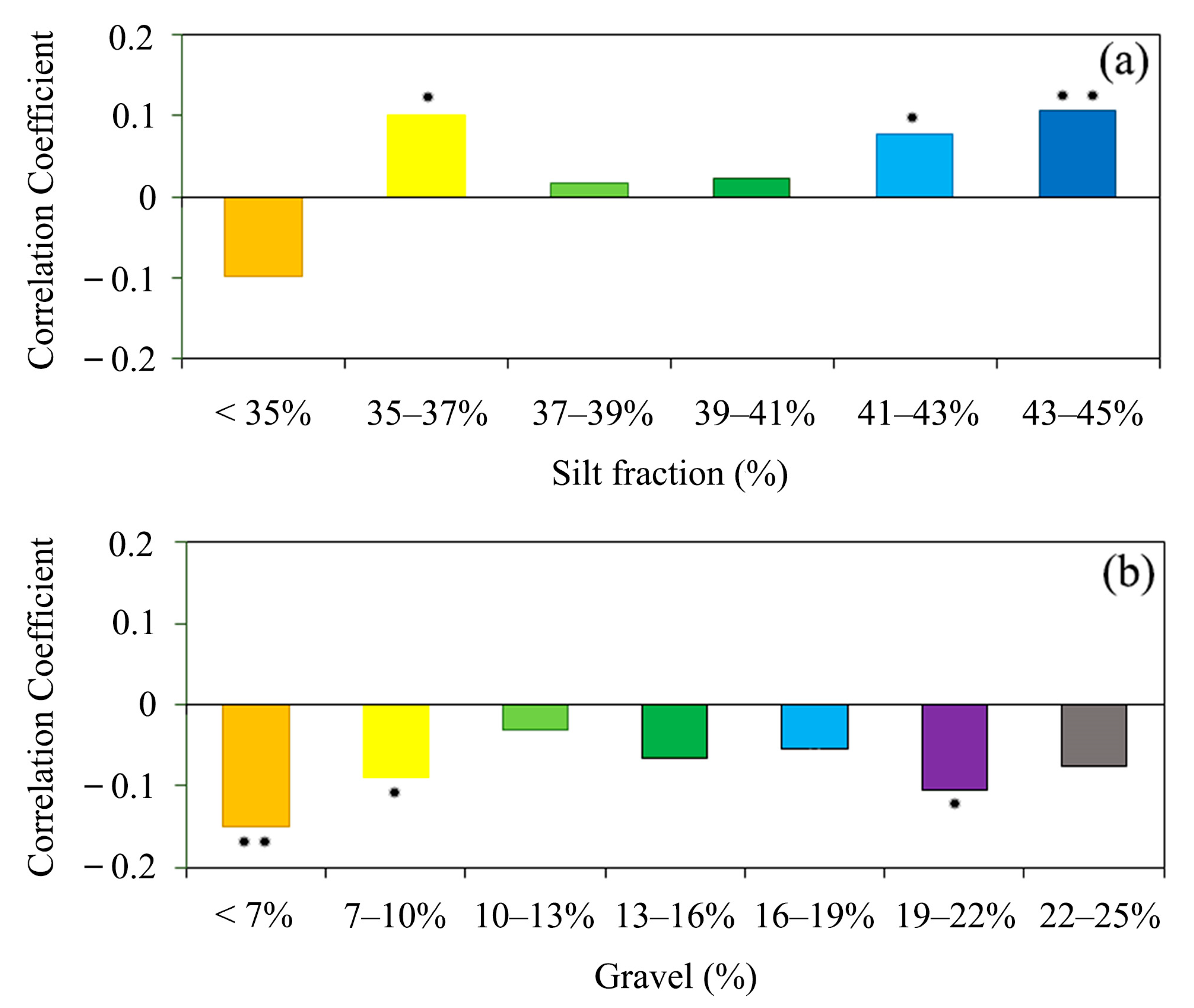
3.4.2. Effects of Environmental Factors on the Vegetation Response to Drought Stress
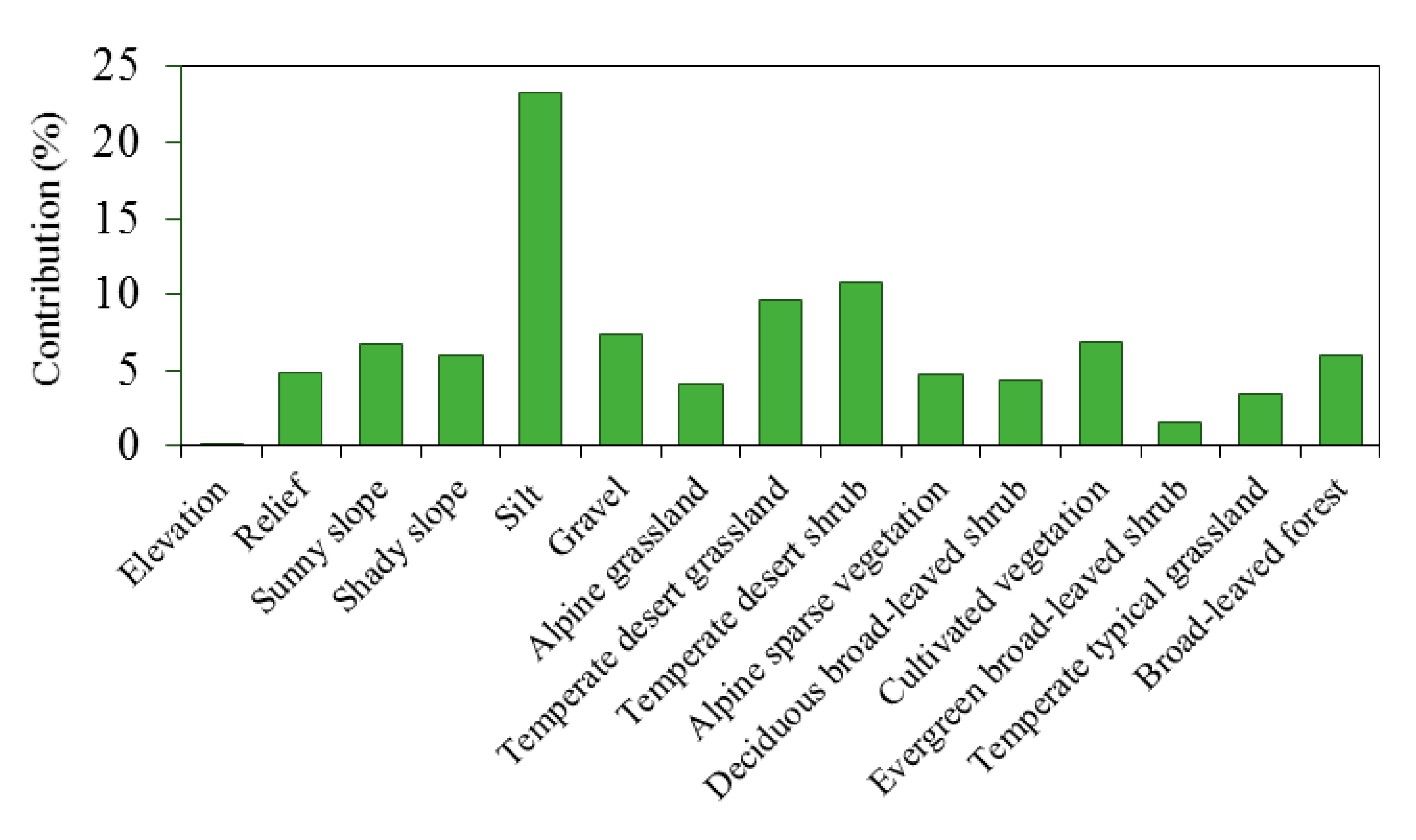
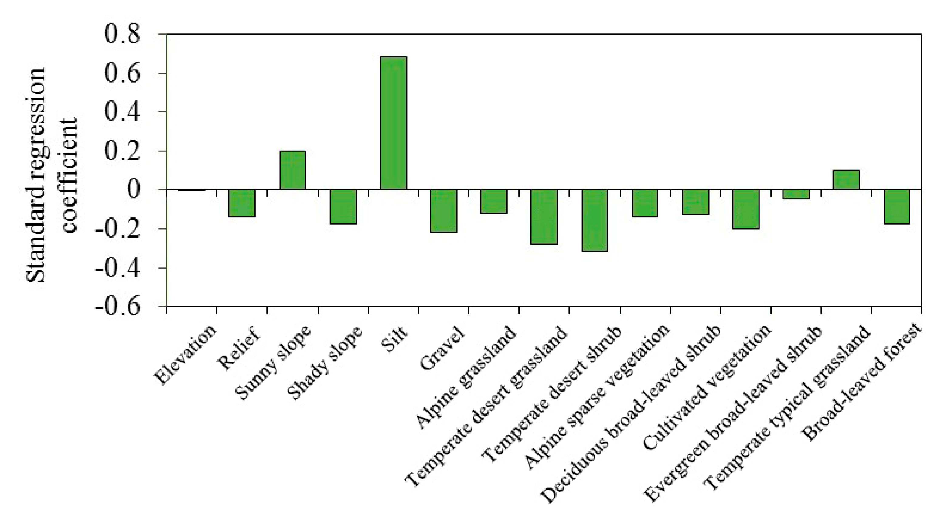
3.4.3. Relative Contributions of Environmental Factors to AI
4. Discussion
4.1. Regional Climate Characteristics
4.2. Effects of Environmental Factors on Vegetation Responses to Drought Stress
5. Conclusions
Author Contributions
Funding
Acknowledgments
Conflicts of Interest
References
- Mishra, A.K.; Singh, V.P. A review of drought concepts. J. Hydrol. 2010, 391, 202–216. [Google Scholar] [CrossRef]
- Li, J.; Wang, Z.; Lai, C. Severe drought events inducing large decrease of net primary productivity in mainland China during 1982. Sci. Total Environ. 2020, 703, 135541. [Google Scholar] [CrossRef] [PubMed]
- Neilson, R.P. A Model for Predicting Continental-Scale Vegetation Distribution and Water Balance. Ecol. Appl. 1995, 5, 362–385. [Google Scholar] [CrossRef]
- Churkina, G.; Running, S.W. Contrasting Climatic Controls on the Estimated Productivity of Global Terrestrial Biomes. Ecosystems 1998, 1, 206–215. [Google Scholar] [CrossRef]
- Zhao, M.; Running, S.W. Drought-Induced Reduction in Global Terrestrial Net Primary Production from 2000 through 2009. Science 2010, 329, 940–943. [Google Scholar] [CrossRef] [PubMed] [Green Version]
- Assal, T.J.; Anderson, P.J.; Sibold, J. Spatial and temporal trends of drought effects in a heterogeneous semi-arid forest ecosystem. For. Ecol. Manag. 2016, 365, 137–151. [Google Scholar] [CrossRef] [Green Version]
- Xu, H.-J.; Wang, X.-P.; Zhao, C.-Y.; Zhang, X.-X. Responses of ecosystem water use efficiency to meteorological drought under different biomes and drought magnitudes in northern China. Agric. For. Meteorol. 2019, 278, 107660. [Google Scholar] [CrossRef]
- Xu, K.; Yang, D.; Yang, H.; Li, Z.; Qin, Y.; Shen, Y. Spatio-temporal variation of drought in China during 1961–2012: A climatic perspective. J. Hydrol. 2015, 526, 253–264. [Google Scholar] [CrossRef]
- Guo, Y.; Huang, S.; Huang, Q.; Leng, G.; Fang, W.; Wang, L.; Wang, H. Propagation thresholds of meteorological drought for triggering hydrological drought at various levels. Sci. Total Environ. 2020, 712, 136502. [Google Scholar] [CrossRef]
- Guo, B.; Chen, Z.; Guo, J.; Liu, F.; Chen, C.; Liu, K. Analysis of the Nonlinear Trends and Non-Stationary Oscillations of Regional Precipitation in Xinjiang, Northwestern China, Using Ensemble Empirical Mode Decomposition. Int. J. Environ. Res. Public Heal. 2016, 13, 345. [Google Scholar] [CrossRef]
- Wu, J.; Chen, X.; Yao, H.; Gao, L.; Chen, Y.; Liu, M. Non-linear relationship of hydrological drought responding to meteorological drought and impact of a large reservoir. J. Hydrol. 2017, 551, 495–507. [Google Scholar] [CrossRef]
- Wang, W.; Zhu, Y.; Xu, R.; Liu, J. Drought severity change in China during 1961–2012 indicated by SPI and SPEI. Nat. Hazards 2015, 75, 2437–2451. [Google Scholar] [CrossRef]
- Tatli, H.; Türkeş, M. Empirical Orthogonal Function analysis of the palmer drought indices. Agric. For. Meteorol. 2011, 151, 981–991. [Google Scholar] [CrossRef]
- Merino, A.; López, L.; Hermida, L.; Sanchez, J.L.; García-Ortega, E.; Gascón, E.; Fernández-González, S. Identification of drought phases in a 110-year record from Western Mediterranean basin: Trends, anomalies and periodicity analysis for Iberian Peninsula. Glob. Planet. Chang. 2015, 133, 96–108. [Google Scholar] [CrossRef]
- Xia, J.; Yang, P.; Zhan, C.; Qiao, Y. Analysis of changes in drought and terrestrial water storage in the Tarim River Basin based on principal component analysis. Hydrol. Res. 2019, 50, 761–777. [Google Scholar] [CrossRef]
- Lloyd-Hughes, B. A spatio-temporal structure-based approach to drought characterisation. Int. J. Clim. 2011, 32, 406–418. [Google Scholar] [CrossRef] [Green Version]
- Andreadis, K.M.; Clark, E.; Wood, A.W.; Hamlet, A.F.; Lettenmaier, D.P. Twentieth-Century Drought in the Conterminous United States. J. Hydrometeorol. 2005, 6, 985–1001. [Google Scholar] [CrossRef]
- Yao, N.; Li, Y.; Lei, T.; Peng, L. Drought evolution, severity and trends in mainland China over 1961–2013. Sci. Total Environ. 2018, 73–89. [Google Scholar] [CrossRef]
- McKee, T.; Doesken, N.; Kleist, J. The Relationship of Drought Frequency and Duration to Time Scales. Proceedings of the 8th Conference on Applied Climatology; American Meteorology Society: Los Angeles, CA, USA, 1993. [Google Scholar]
- Vicente-Serrano, S.M.; Beguería, S.; López-Moreno, J.I. A Multiscalar Drought Index Sensitive to Global Warming: The Standardized Precipitation Evapotranspiration Index. J. Clim. 2010, 23, 1696–1718. [Google Scholar] [CrossRef] [Green Version]
- Zhang, B.; Long, B.; Wu, Z.; Wang, Z. An Evaluation of the Performance and the Contribution of Different Modified Water Demand Estimates in Drought Modeling Over Water-stressed Regions. Land Degrad. Dev. 2017, 28, 1134–1151. [Google Scholar] [CrossRef]
- Tian, L.; Yuan, S.; Quiring, S.M. Evaluation of six indices for monitoring agricultural drought in the south-central United States. Agric. For. Meteorol. 2018, 249, 107–119. [Google Scholar] [CrossRef]
- Nanzad, L.; Zhang, J.; Tuvdendorj, B.; Nabil, M.; Zhang, S.; Bai, Y. NDVI anomaly for drought monitoring and its correlation with climate factors over Mongolia from 2000 to 2016. J. Arid. Environ. 2019, 164, 69–77. [Google Scholar] [CrossRef]
- Tian, F.; Fensholt, R.; Verbesselt, J.; Grogan, K.; Horion, S.; Wang, Y. Evaluating temporal consistency of long-term global NDVI datasets for trend analysis. Remote Sens. Environ. 2015, 163, 326–340. [Google Scholar] [CrossRef]
- Zhao, Z.; Zhang, Y.; Liu, L.-S.; Hu, Z. The impact of drought on vegetation conditions within the Damqu River Basin, Yangtze River Source Region, China. PLoS ONE 2018, 13, e0202966. [Google Scholar] [CrossRef] [PubMed]
- Vicente-Serrano, S.M.; Gouveia, C.; Camarero, J.J.; Beguería, S.; Trigo, R.M.; López-Moreno, J.I.; Azorín-Molina, C.; Pasho, E.; Lorenzo-Lacruz, J.; Revuelto, J.; et al. Response of vegetation to drought time-scales across global land biomes. Proc. Natl. Acad. Sci. USA 2013, 110, 52–57. [Google Scholar] [CrossRef] [Green Version]
- Ji, L.; Peters, A.J. Assessing vegetation response to drought in the northern Great Plains using vegetation and drought indices. Remote Sens. Environ. 2003, 87, 85–98. [Google Scholar] [CrossRef]
- Meroni, M.; Fasbender, D.; Rembold, F.; Atzberger, C.; Klisch, A. Near real-time vegetation anomaly detection with MODIS NDVI: Timeliness vs. accuracy and effect of anomaly computation options. Remote Sens. Environ. 2019, 221, 508–521. [Google Scholar] [CrossRef]
- Zhao, Y.-Z.; Zou, X.-Y.; Cheng, H.; Jia, H.-K.; Wu, Y.-Q.; Wang, G.-Y.; Zhang, C.; Gao, S.-Y. Assessing the ecological security of the Tibetan plateau: Methodology and a case study for Lhaze County. J. Environ. Manag. 2006, 80, 120–131. [Google Scholar] [CrossRef]
- Li, B.; Zhou, W.; Zhao, Y.; Ju, Q.; Yu, Z.; Liang, Z.; Acharya, K. Using the SPEI to Assess Recent Climate Change in the Yarlung Zangbo River Basin, South Tibet. Water 2015, 7, 5474–5486. [Google Scholar] [CrossRef] [Green Version]
- Li, X.; Liu, L.; Shan, B.; Xu, Z.; Niu, Q.; Cheng, L.; Liu, X.; Xu, Z. Spatiotemporal Variation of Drought and Associated Multi-Scale Response to Climate Change over the Yarlung Zangbo River Basin of Qinghai–Tibet Plateau, China. Remote Sens. 2019, 11, 1596. [Google Scholar] [CrossRef] [Green Version]
- Liu, D.; Wang, T.; Yang, T.; Yan, Z.; Liu, Y.; Zhao, Y.; Piao, S. Deciphering impacts of climate extremes on Tibetan grasslands in the last fifteen years. Sci. Bull. 2019, 64, 446–454. [Google Scholar] [CrossRef] [Green Version]
- Lu, D. Runoff Prediction and Research in Middle Reaches of Yarlung Zangbo River. Master’s Thesis, Sichuan University, Chengdu, China, 2006. [Google Scholar]
- Zheng, Y.; Zhang, L.; Xiao, J.; Yuan, W.; Yan, M.; Li, T.; Zhang, Z. Sources of uncertainty in gross primary productivity simulated by light use efficiency models: Model structure, parameters, input data, and spatial resolution. Agric. For. Meteorol. 2018, 263, 242–257. [Google Scholar] [CrossRef]
- Wang, Y.; Wesche, K. Vegetation and soil responses to livestock grazing in Central Asian grasslands: A review of Chinese literature. Biodivers. Conserv. 2016, 25, 2401–2420. [Google Scholar] [CrossRef]
- Wang, X.; Chai, K.; Liu, S.; Wei, J.; Jiang, Z.; Liu, Q. Changes of glaciers and glacial lakes implying corridor-barrier effects and climate change in the Hengduan Shan, southeastern Tibetan Plateau. J. Glaciol. 2017, 63, 535–542. [Google Scholar] [CrossRef] [Green Version]
- Sims, D.A.; Gamon, J.A. Relationships between leaf pigment content and spectral reflectance across a wide range of species, leaf structures and developmental stages. Remote Sens. Environ. 2002, 81, 337–354. [Google Scholar] [CrossRef]
- Grace, J.; Nichol, C.; Disney, M.; Lewis, P.; Quaife, T.; Bowyer, P. Can we measure terrestrial photosynthesis from space directly, using spectral reflectance and fluorescence? Glob. Chang. Biol. 2007, 13, 1484–1497. [Google Scholar] [CrossRef]
- Mänd, P.; Hallik, L.; Peñuelas, J.; Nilson, T.; Duce, P.; Emmett, B.A.; Beier, C.; Estiarte, M.; Garadnai, J.; Kalapos, T.; et al. Responses of the reflectance indices PRI and NDVI to experimental warming and drought in European shrublands along a north–south climatic gradient. Remote Sens. Environ. 2010, 114, 626–636. [Google Scholar] [CrossRef]
- Pinzon, J.E.; Brown, M.E.; Tucker, C.J.; Huang, N.E.; Shen, S.S.P. EMD Correction of Orbital Drift Artifacts in Satellite Data Stream. Hilbert-Huang Transform. Appl. 2014, 8, 241–260. [Google Scholar] [CrossRef]
- Tucker, C.J.; Slayback, D.A.; Pinzon, J.E.; Los, S.O.; Myneni, R.B.; Taylor, M.G. Higher northern latitude normalized difference vegetation index and growing season trends from 1982 to 1999. Int. J. Biometeorol. 2001, 45, 184–190. [Google Scholar] [CrossRef]
- Jiang, B.; Liang, S.; Yuan, W. Observational evidence for impacts of vegetation change on local surface climate over northern China using the Granger causality test. J. Geophys. Res. Biogeosci. 2015, 120, 1–12. [Google Scholar] [CrossRef]
- Ng, E.; Miller, P.C. Soil Moisture Relations in the Southern California Chaparral. Ecology 1980, 61, 98–107. [Google Scholar] [CrossRef]
- Gómez-Plaza, A.; Martínez-Mena, M.; Albaladejo, J.; Castillo, V.M. Factors regulating spatial distribution of soil water content in small semiarid catchments. J. Hydrol. 2001, 253, 211–226. [Google Scholar] [CrossRef]
- Fernandez-Illescas, C.P.; Porporato, A.; Laio, F.; Rodriguez-Iturbe, I. The ecohydrological role of soil texture in a water-limited ecosystem. Water Resour. Res. 2001, 37, 2863–2872. [Google Scholar] [CrossRef]
- Okin, G.S.; Dong, C.; Willis, K.S.; Gillespie, T.W.; Macdonald, G. The Impact of Drought on Native Southern California Vegetation: Remote Sensing Analysis Using MODIS-Derived Time Series. J. Geophys. Res. Biogeosci. 2018, 123, 1927–1939. [Google Scholar] [CrossRef]
- Zhang, B.; He, C. A modified water demand estimation method for drought identification over arid and semiarid regions. Agric. For. Meteorol. 2016, 58–66. [Google Scholar] [CrossRef]
- Wang, X.; Zhuo, L.; Li, C.A.; Engel, B.; Sun, S.; Wang, Y. Temporal and spatial evolution trends of drought in northern Shaanxi of China: 1960–2100. Theor. Appl. Clim. 2020, 139, 965–979. [Google Scholar] [CrossRef]
- Das, P.K.; Chandra, S.; Das, D.K.; Midya, S.K.; Paul, A.; Bandyopadhyay, S.; Dadhwal, V.K. Understanding the interactions between meteorological and soil moisture drought over Indian region. J. Earth Syst. Sci. 2020, 129, 1–17. [Google Scholar] [CrossRef]
- Wang, H.; He, B.; Zhang, Y.; Huang, L.; Chen, Z.; Liu, J. Response of ecosystem productivity to dry/wet conditions indicated by different drought indices. Sci. Total. Environ. 2018, 612, 347–357. [Google Scholar] [CrossRef]
- Fung, K.F.; Huang, Y.F.; Koo, C.H. Assessing drought conditions through temporal pattern, spatial characteristic and operational accuracy indicated by SPI and SPEI: Case analysis for Peninsular Malaysia. Nat. Hazards 2020, 103, 2071–2101. [Google Scholar] [CrossRef]
- R Core Team. A Language and Environment for Statistical Computing; R Foundation for Statistical Computing: Vienna, Austria, 2016; Available online: https://www.gbif.org/tool/81287/r-a-language-and-environment-for-statistical-computing (accessed on 18 December 2020).
- Herrera-Estrada, J.E.; Satoh, Y.; Sheffield, J. Spatiotemporal dynamics of global drought. Geophys. Res. Lett. 2017, 44, 2254–2263. [Google Scholar] [CrossRef] [Green Version]
- Guo, H.; Bao, A.; Ndayisaba, F.; Liu, T.; Jiapaer, G.; El-Tantawi, A.M.; De Maeyer, P. Space-time characterization of drought events and their impacts on vegetation in Central Asia. J. Hydrol. 2018, 564, 1165–1178. [Google Scholar] [CrossRef]
- Chen, H.; Sun, J. Changes in Drought Characteristics over China Using the Standardized Precipitation Evapotranspiration Index. J. Clim. 2015, 28, 5430–5447. [Google Scholar] [CrossRef]
- Li, J.; Wang, Z.; Wu, X.; Chen, J.; Guo, S.; Zhang, Z. A new framework for tracking flash drought events in space and time. Catena 2020, 194, 104763. [Google Scholar] [CrossRef]
- Xu, K.; Yang, D.; Xu, X.; Lei, H. Copula based drought frequency analysis considering the spatio-temporal variability in Southwest China. J. Hydrol. 2015, 527, 630–640. [Google Scholar] [CrossRef]
- Zhou, H.; Liu, Y.; Liu, Y. An Approach to Tracking Meteorological Drought Migration. Water Resour. Res. 2019, 55, 3266–3284. [Google Scholar] [CrossRef]
- Wang, A.; Lettenmaier, D.P.; Sheffield, J. Soil Moisture Drought in China, 1950–2006. J. Clim. 2011, 24, 3257–3271. [Google Scholar] [CrossRef]
- Zhu, Z.; Piao, S.; Myneni, R.B.; Huang, M.; Zeng, Z.; Canadell, J.G.; Ciais, P.; Sitch, S.; Friedlingstein, P.; Arneth, A.; et al. Greening of the Earth and its drivers. Nat. Clim. Chang. 2016, 6, 791–795. [Google Scholar] [CrossRef]
- Seddon, A.W.R.; Macias-Fauria, M.; Long, P.R.; Benz, D.; Willis, K.J. Sensitivity of global terrestrial ecosystems to climate variability. Nat. Cell Biol. 2016, 531, 229–232. [Google Scholar] [CrossRef] [Green Version]
- Chen, W.; Huang, C.; Wang, L.; Li, D. Climate Extremes and Their Impacts on Interannual Vegetation Variabilities: A Case Study in Hubei Province of Central China. Remote Sens. 2018, 10, 477. [Google Scholar] [CrossRef] [Green Version]
- Wang, Y.; Yang, K.; Pan, Z.; Qin, J.; Chen, D.; Lin, C.; Chen, Y.; Tang, W.; Han, M.; Lu, N.; et al. Evaluation of Precipitable Water Vapor from Four Satellite Products and Four Reanalysis Datasets against GPS Measurements on the Southern Tibetan Plateau. J. Clim. 2017, 30, 5699–5713. [Google Scholar] [CrossRef]
- Knapp, A.K.; Beier, C.; Briske, D.D.; Classen, A.T.; Luo, Y.; Reichstein, M.; Smith, M.D.; Smith, S.D.; Bell, J.E.; Fay, P.A.; et al. Consequences of More Extreme Precipitation Regimes for Terrestrial Ecosystems. Bioscience 2008, 58, 811–821. [Google Scholar] [CrossRef]
- Chaves, M.; Maroco, J.P.; Pereira, J.S. Understanding plant responses to drought—From genes to the whole plant. Funct. Plant Biol. 2003, 30, 239–264. [Google Scholar] [CrossRef] [PubMed]
- Tao, J.; Zhang, Y.; Dong, J.; Fu, Y.; Zhu, J.; Zhang, G.; Jiang, Y.; Tian, L.; Zhang, X.; Zhang, T.; et al. Elevation-dependent relationships between climate change and grassland vegetation variation across the Qinghai-Xizang Plateau. Int. J. Clim. 2014, 35, 1638–1647. [Google Scholar] [CrossRef] [Green Version]
- Li, P.; Zhu, D.; Wang, Y.; Liu, D. Elevation dependence of drought legacy effects on vegetation greenness over the Tibetan Plateau. Agric. For. Meteorol. 2020, 295, 108190. [Google Scholar] [CrossRef]
- Walters, J.T.; McNider, R.T.; Shi, X.; Norris, W.B.; Christy, J.R. Positive surface temperature feedback in the stable nocturnal boundary layer. Geophys. Res. Lett. 2007, 34, 237–254. [Google Scholar] [CrossRef]
- Noymeir, I. Desert Ecosystems: Environment and Producers. Annu. Rev. Ecol. Syst. 1973, 4, 25–51. [Google Scholar] [CrossRef]
- Zhu, X.; Bothe, O.; Fraedrich, K. Summer atmospheric bridging between Europe and East Asia: Influences on drought and wetness on the Tibetan Plateau. Quat. Int. 2011, 236, 151–157. [Google Scholar] [CrossRef]
- Wang, Z.; Li, J.; Lai, C.; Zeng, Z.; Zhong, R.; Chen, X.; Zhou, X.; Wang, M. Does drought in China show a significant decreasing trend from 1961 to 2009? Sci. Total Environ. 2017, 579, 314–324. [Google Scholar] [CrossRef]
- Krishnan, R.; Sugi, M. Pacific decadal oscillation and variability of the Indian summer monsoon rainfall. Clim. Dyn. 2003, 21, 233–242. [Google Scholar] [CrossRef]
- Liu, X.; Yin, Z.-Y. Spatial and Temporal Variation of Summer Precipitation over the Eastern Tibetan Plateau and the North Atlantic Oscillation. J. Clim. 2001, 14, 2896–2909. [Google Scholar] [CrossRef] [Green Version]
- Lechuga, V.; Carraro, V.; Viñegla, B.; Carreira, J.A.; Linares, J.C. Carbon Limitation and Drought Sensitivity at Contrasting Elevation and Competition of Abies pinsapo Forests. Does Experimental Thinning Enhance Water Supply and Carbohydrates? Forests 2019, 10, 1132. [Google Scholar] [CrossRef] [Green Version]
- De Keersmaecker, W.; Lhermitte, S.; Tits, L.; Honnay, O.; Somers, B.; Coppin, P. A model quantifying global vegetation resistance and resilience to short-term climate anomalies and their relationship with vegetation cover. Glob. Ecol. Biogeogr. 2015, 24, 539–548. [Google Scholar] [CrossRef]
- Jiang, Y.; Wang, R.; Peng, Q.; Wu, X.; Ning, H.; Li, C. The relationship between drought activity and vegetation cover in Northwest China from 1982 to 2013. Nat. Hazards 2018, 92, 145–163. [Google Scholar] [CrossRef]
- Ponce-Campos, G.E.; Moran, M.S.; Huete, A.; Zhang, Y.; Bresloff, C.; Huxman, T.E.; Eamus, D.; Bosch, D.D.; Buda, A.R.; Gunter, S.A.; et al. Ecosystem resilience despite large-scale altered hydroclimatic conditions. Nat. Cell Biol. 2013, 494, 349–352. [Google Scholar] [CrossRef] [PubMed]
- Wu, J.; Zhang, X.; Shen, Z.; Shi, P.; Xu, X.; Li, X. Grazing-Exclusion Effects on Aboveground Biomass and Water-Use Efficiency of Alpine Grasslands on the Northern Tibetan Plateau. Rangel. Ecol. Manag. 2013, 66, 454–461. [Google Scholar] [CrossRef]
- Trifilò, P.; Casolo, V.; Raimondo, F.; Petrussa, E.; Boscutti, F.; Gullo, M.A.L.; Nardini, A. Effects of prolonged drought on stem non-structural carbohydrates content and post-drought hydraulic recovery in Laurus nobilis L.: The possible link between carbon starvation and hydraulic failure. Plant Physiol. Biochem. 2017, 120, 232–241. [Google Scholar] [CrossRef]
- Li, Q.; Zhao, M.; Wang, N.; Liu, S.; Wang, J.; Zhang, W.; Yang, N.; Fan, P.; Wang, R.; Wang, H.; et al. Water use strategies and drought intensity define the relative contributions of hydraulic failure and carbohydrate depletion during seedling mortality. Plant Physiol. Biochem. 2020, 153, 106–118. [Google Scholar] [CrossRef]
- Dodd, M.B.; Lauenroth, W.; Burke, I.; Chapman, P. Associations between vegetation patterns and soil texture in the shortgrass steppe. Plant Ecol. 2002, 158, 127–137. [Google Scholar] [CrossRef]
- Duan, D.-Y.; Ouyang, H.; Song, M.-H.; Hu, Q.-W. Water Sources of Dominant Species in Three Alpine Ecosystems on the Tibetan Plateau, China. J. Integr. Plant Biol. 2008, 50, 257–264. [Google Scholar] [CrossRef]
- Li, Z.; Zhou, T.; Zhao, X.; Huang, K.; Gao, S.; Wu, H.; Luo, H. Assessments of Drought Impacts on Vegetation in China with the Optimal Time Scales of the Climatic Drought Index. Int. J. Environ. Res. Public Health 2015, 12, 7615–7634. [Google Scholar] [CrossRef] [Green Version]
- Zhao, A.; Zhang, A.; Cao, S.; Liu, X.; Liu, J.; Cheng, D. Responses of vegetation productivity to multi-scale drought in Loess Plateau, China. Catena 2018, 163, 165–171. [Google Scholar] [CrossRef]
- Zhang, Q.; Kong, D.; Singh, V.P.; Shi, P. Response of vegetation to different time-scales drought across China: Spatiotemporal patterns, causes and implications. Glob. Planet. Chang. 2017, 152, 1–11. [Google Scholar] [CrossRef] [Green Version]
- Baldocchi, D.D.; Xu, L.; Kiang, N. How plant functional-type, weather, seasonal drought, and soil physical properties alter water and energy fluxes of an oak–grass savanna and an annual grassland. Agric. For. Meteorol. 2004, 123, 13–39. [Google Scholar] [CrossRef] [Green Version]
- Wolf, S.; Eugster, W.; Ammann, C.; Häni, M.; Zielis, S.; Hiller, R.; Stieger, J.; Imer, D.; Merbold, L.; Buchmann, N. Contrasting response of grassland versus forest carbon and water fluxes to spring drought in Switzerland. Environ. Res. Lett. 2013, 8, 035007. [Google Scholar] [CrossRef] [Green Version]
- Stuart-Haëntjens, E.; De Boeck, H.J.; Lemoine, N.P.; Mänd, P.; Kröel-Dulay, G.; Schmidt, I.K.; Jentsch, A.; Stampfli, A.; Anderegg, W.R.; Bahn, M.; et al. Mean annual precipitation predicts primary production resistance and resilience to extreme drought. Sci. Total Environ. 2018, 636, 360–366. [Google Scholar] [CrossRef] [PubMed]


| Classification and Data Source | Temporal Resolution | Spatial Resolution | Description |
|---|---|---|---|
| Climate variables westdc.westgis.ac.cn/data | 3 h | 9 km | Precipitation |
| Vegetation indexes http://ecocast.arc.nasa.gov/data/pub/ | 15 d | 8 km | NDVI (normalized difference vegetation index) |
| Soil variables https://data.tpdc.ac.cn/zh-hans/ | - | 1 km | Soil texture (i.e., sandy soil, silt soil, clay soil and gravel) |
| Topographic variables http://www.gscloud.cn | - | 90 m | Altitude, relief, and aspect |
| Vegetation types http://www.resdc.cn | - (vector) | - (vector) | Basic vegetation types |
| SPI Intervals | SPI Classes |
|---|---|
| SPI > 2 | Extremely wet |
| 2 > SPI > 1.5 | Severely wet |
| 1.5 > SPI > 1 | Moderately wet |
| 1 > SPI > −1 | Normal |
| −1 > SPI > −1.5 | Moderately dry |
| −1.5 > SPI > −2 | Severity dry |
| SPI < −2 | Extremely dry |
| Model | Coefficients | t-Test | p-Value | VIF | |
|---|---|---|---|---|---|
| B | SE | ||||
| Constant | 37 | 4.098 | 9.249 | 3.36 × 10⁻²⁰ | |
| Elevation | −0.005 | 0.000 | −11.808 | 9.85 × 10⁻³² | 5.772 |
| Relief | −0.142 | 0.022 | −6.464 | 1.12 × 10⁻¹⁰ | 2.732 |
| Sunny slope | 0.198 | 0.042 | 4.694 | 2.75 × 10⁻⁶ | 1.354 |
| Shady slope | −0.175 | 0.053 | −3.28 | 1.00 × 10⁻³ | 1.4 |
| Silt | 0.68 | 0.08 | 8.397 | 6.00 × 10⁻¹⁷ | 2.035 |
| Gravel | −0.216 | 0.045 | −4.845 | 1.30 × 10⁻⁶ | 1.768 |
| Alpine grassland | −0.118 | 0.01 | −12.27 | 4.15 × 10⁻³⁴ | 1.94 |
| Temperate desert grassland | −0.28 | 0.016 | −18.05 | 1.73 × 10−70 | 1.239 |
| Temperate desert shrub | −0.316 | 0.024 | −13.4 | 3.00 × 10−40 | 1.17 |
| Alpine sparse vegetation | −0.139 | 0.011 | −12.65 | 4.03 × 10−36 | 2.45 |
| Deciduous broad-leaved shrub | −0.128 | 0.023 | −5.55 | 3.00 × 10⁻⁸ | 1.085 |
| Cultivated vegetation | −0.202 | 0.038 | −5.327 | 1.04 × 10⁻⁷ | 1.41 |
| Evergreen broad-leaved shrub | −0.044 | 0.011 | −3.95 | 8.00 × 10⁻⁵ | 1.457 |
| Temperate typical grassland | 0.1 | 0.024 | 4.14 | 3.49 × 10⁻⁵ | 1.19 |
| Broad-leaved forest | −0.176 | 0.027 | −6.55 | 6.23 × 10⁻¹¹ | 2.206 |
Publisher’s Note: MDPI stays neutral with regard to jurisdictional claims in published maps and institutional affiliations. |
© 2020 by the authors. Licensee MDPI, Basel, Switzerland. This article is an open access article distributed under the terms and conditions of the Creative Commons Attribution (CC BY) license (http://creativecommons.org/licenses/by/4.0/).
Share and Cite
Ye, Z.-X.; Cheng, W.-M.; Zhao, Z.-Q.; Guo, J.-Y.; Yang, Z.-X.; Wang, R.-B.; Wang, N. Spatio-Temporal Characteristics of Drought Events and Their Effects on Vegetation: A Case Study in Southern Tibet, China. Remote Sens. 2020, 12, 4174. https://0-doi-org.brum.beds.ac.uk/10.3390/rs12244174
Ye Z-X, Cheng W-M, Zhao Z-Q, Guo J-Y, Yang Z-X, Wang R-B, Wang N. Spatio-Temporal Characteristics of Drought Events and Their Effects on Vegetation: A Case Study in Southern Tibet, China. Remote Sensing. 2020; 12(24):4174. https://0-doi-org.brum.beds.ac.uk/10.3390/rs12244174
Chicago/Turabian StyleYe, Zu-Xin, Wei-Ming Cheng, Zhi-Qi Zhao, Jian-Yang Guo, Ze-Xian Yang, Rui-Bo Wang, and Nan Wang. 2020. "Spatio-Temporal Characteristics of Drought Events and Their Effects on Vegetation: A Case Study in Southern Tibet, China" Remote Sensing 12, no. 24: 4174. https://0-doi-org.brum.beds.ac.uk/10.3390/rs12244174