Retrieving Surface Soil Water Content Using a Soil Texture Adjusted Vegetation Index and Unmanned Aerial System Images


1
Department of Plant and Soil Science, Texas Tech University, Lubbock, TX 79409, USA
2
Department of Soil and Crop Sciences, Texas A&M AgriLife Research, Lubbock, TX 79403, USA
*
Author to whom correspondence should be addressed.
Remote Sens. 2021, 13(1), 145; https://0-doi-org.brum.beds.ac.uk/10.3390/rs13010145
Submission received: 1 December 2020
/
Revised: 28 December 2020
/
Accepted: 30 December 2020
/
Published: 4 January 2021
(This article belongs to the Special Issue Drones for Precision Agriculture: Remote Sensing Applications)
Abstract
:Surface soil water content (SWC) is a major determinant of crop production, and accurately retrieving SWC plays a crucial role in effective water management. Unmanned aerial systems (UAS) can acquire images with high temporal and spatial resolutions for SWC monitoring at the field scale. The objective of this study was to develop an algorithm to retrieve SWC by integrating soil texture into a vegetation index derived from UAS multispectral and thermal images. The normalized difference vegetation index (NDVI) and surface temperature (Ts) derived from the UAS multispectral and thermal images were employed to construct the temperature vegetation dryness index (TVDI) using the trapezoid model. Soil texture was incorporated into the trapezoid model based on the relationship between soil texture and the lower and upper limits of SWC to form the texture temperature vegetation dryness index (TTVDI). For validation, 128 surface soil samples, 84 in 2019 and 44 in 2020, were collected to determine soil texture and gravimetric SWC. Based on the linear regression models, the TTVDI had better performance in estimating SWC compared to the TVDI, with an increase in R2 (coefficient of determination) by 14.5% and 14.9%, and a decrease in RMSE (root mean square error) by 46.1% and 10.8%, for the 2019 and 2020 samples, respectively. The application of the TTVDI model based on high-resolution multispectral and thermal UAS images has the potential to accurately and timely retrieve SWC at the field scale.
1. Introduction
The surface soil water content (SWC) constitutes a small portion of the agroecosystem, but it plays a critical role in agricultural production [1,2]. Accurate estimation of surface SWC is indispensable in ecology, hydrology, climatology, and environmental and agricultural water management [3,4,5,6,7]. Different methods have been used to measure or estimate SWC, including field measurements, remote sensing, and soil water balance simulation models [8,9,10,11]. Compared with the cost-prohibitive, labor-intensive, and time-consuming in-situ measurements and complex model predictions, remote sensing technology has demonstrated great potential for estimating and monitoring surface SWC for its timeliness and convenience at larger spatial scales [12]. For instance, studies have reported that satellite data, such as those from MODIS, Landsat, and Sentinel l/2, in the wavelengths of near-infrared, thermal infrared, and microwave, can be applied to monitor SWC at different scales [1,6,13].
Based on various satellite data, a wide variety of models for estimating surface SWC have been developed over the past decades [14,15,16,17]. For instance, Nemani et al. (1993) developed the temperature vegetation dryness index (TVDI) based on the relationship between the surface temperature (Ts) and the normalized difference vegetation index (NDVI) by plotting NDVI against Ts values [16]. In the TVDI model, temperature changes are mainly explained by the variation in land SWC, i.e., for a given NDVI value, temperature varies mainly as a function of surface SWC change [18,19]. The TVDI model has various applications, such as the estimation of crop water stress, drought, and evapotranspiration [20,21,22,23].
Studies have demonstrated the potential of using the TVDI for SWC estimation at large scales, such as river valley, state, regional, or worldwide [24,25,26,27]. Nevertheless, information on the feasibility of using the TVDI for monitoring surface SWC on the size of a typical agricultural field is very limited [28,29]. This is because the TVDI model requires a large number of pixels with wide ranges of NDVI and Ts values to build the trapezoid model and determine the dry and wet boundary conditions [30]. Satellite data of medium resolutions, such as Landsat (30 m) and Sentinel (20 m) data, and coarse resolutions, such as MODIS data (250–1000 m), cannot provide a sufficiently large number of pixels to build the NDVI and temperature trapezoid model at the field scale [31,32,33]. Although some remote sensing data have high resolutions, they do not contain the thermal bands required for the TVDI calculation. Image re-sampling and down-scaling methods can be employed to improve the applicability of traditional remote sensing images at the field scale [34,35,36]. However, calibrated data based on low-resolution images are often not consistent with the scale of SWC distribution due to the strong spatial variability. Besides, the long revisit time and weather limitation of traditional satellite platforms limit accurate and dynamic monitoring of SWC at the field scale [37,38].
The emergence and development of the unmanned aerial systems (UAS) provide a potential solution to the challenges encountered by traditional remote sensing in real-time and efficient monitoring, especially at the field scale [39,40]. UAS remote sensing systems not only provide high-resolution data at the field scale, but also reduce the limitation of revisit time, weather factors, and operating costs [41,42]. Agricultural managers can use the real-time information obtained from the UAS and combine ground measurements to accomplish more reliable techniques for agricultural monitoring. UAS remote sensing has been applied in agriculture to monitor or predict SWC [43], plant population [44,45], crop water stress [46], crop nutrient deficiency [47,48], plant biomass, leaf area [49,50], and crop yield [51,52].
Although the TVDI model has been used to estimate SWC using UAS images in recent years, its application in estimating SWC only incorporates the spectral characteristics of surface objects without considering the soil properties that affect SWC [27,43,53,54,55]. For instance, soil texture, an important soil parameter affecting SWC, is not considered in the TVDI model [4,56]. Soil texture is a stable soil physical property, and its variation results in large spatial and temporal variability in SWC distribution [57,58]. Besides, soil surface temperature used to estimate SWC in remote sensing studies is also governed by the variation in soil texture [59]. Several authors have found that the upper and lower limits of SWC are a function of soil clay and sand content [43,60,61]. More importantly, the interaction between soil texture and SWC is highly correlated with electromagnetic radiation at various wavelengths, from the visible to the thermal infrared spectral regions [62,63,64]. Amazirh et al. (2018) integrated soil texture in the Sentinel-1 radar and Landsat thermal imagery to improve SWC retrieval accuracy on a large scale [65]. Thus, incorporating the effect of soil texture in the TVDI model has the potential to enhance the SWC retrieval accuracy. To date, no studies have reported the integration of soil texture and the TVDI model in SWC retrieval. At the field scale, the lack of information is equally true for SWC’s timely and accurate retrieval and hinders the development of precision agriculture. Therefore, the objective of this study was to develop a new model that integrates soil texture, Ts, and the NDVI from high-resolution multispectral and thermal UAS images to retrieve SWC at the field scale.
2. Materials and Methods
2.1. Study Area
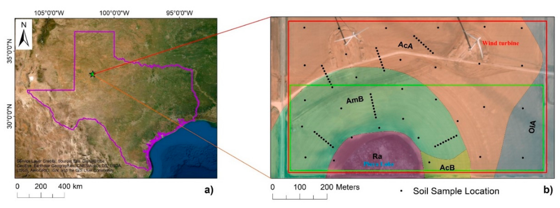
The study was conducted in a dryland field (~40 ha) located 15 km southeast of Slaton (33°19′28.33″ N, 101°33′13.40″ W), Garza County, Texas (Figure 1). The local climate is semiarid, characterized by large diurnal temperature variations and day-to-day variability. The average annual rainfall is 487 mm and the mean annual temperature is 16 °C [66]. The elevation of this field varies from 914 m at the northwest corner to 908 m at the playa lake on the south side. A terrace was constructed in the middle of the field for soil and water conservation. As indicated by the soil map units (Figure 1) from the National Resources Conservation Service (NRCS) Soil Survey Geographic Database (SSURGO), soil types varied from fine sandy loam and loam in the main part of the field, to clay at the playa lake in the south. The study was conducted in the entire field in 2019 (red polygon, ~40 ha), and in the south half in 2020 (green polygon, ~21 ha) due to the construction of wind turbines.
2.2. UAS Platform and Sensors
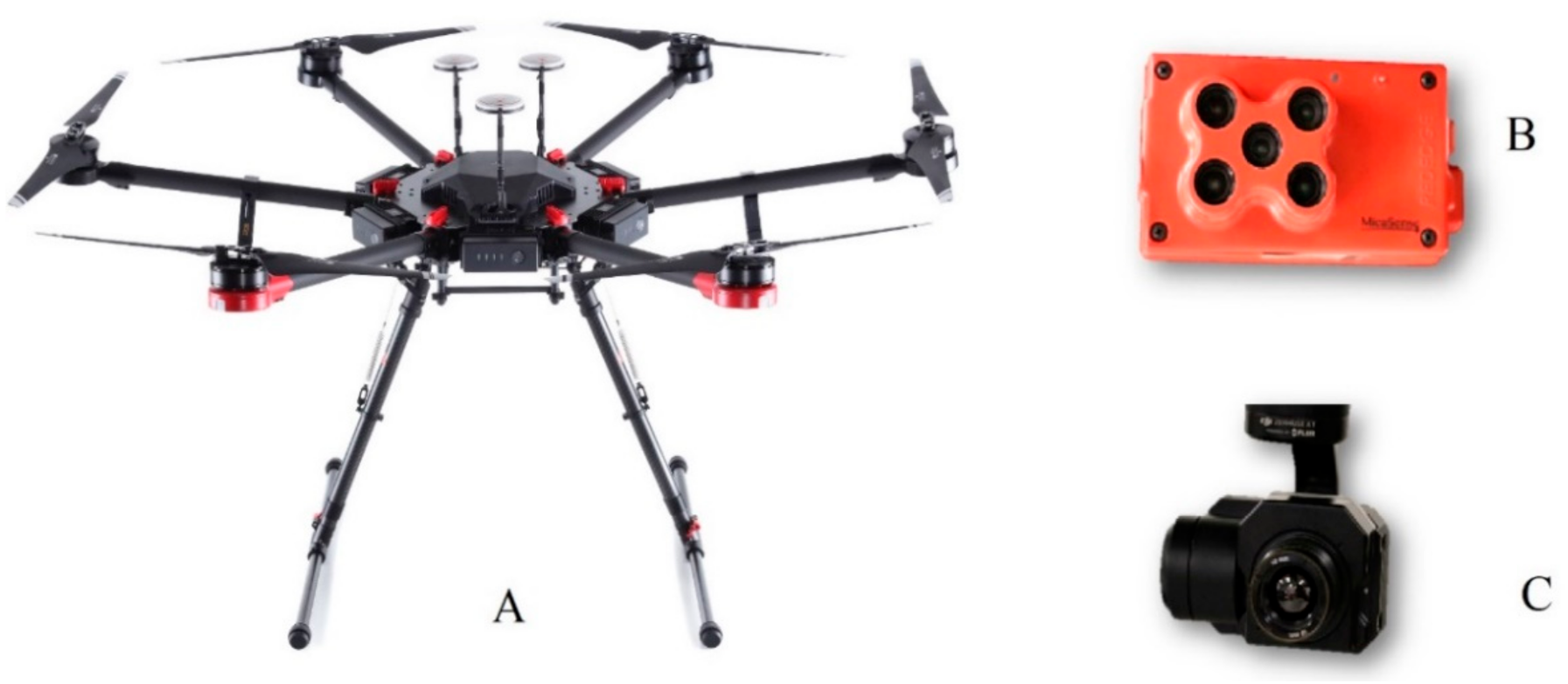
A DJI Matrice 600 UAS (DJI, Shenzhen, China) was applied as a platform for sensors to acquire images (Figure 2). A RedEdge sensor (MicaSense, Seattle, WA, USA) was used to collect multispectral images, with central wavelengths of 475, 560, 668, 717, and 840 nm for the blue, green, red, red edge, and NIR, respectively. A thermal infrared (TIR) sensor (Zenmuse XT, FLIR System, Shenzhen, China) was used to acquire thermal images. This sensor has a dimension of 103 mm × 74 mm × 102 mm, and a weight of 270 g. It is capable of capturing the wavelength range of 7.5 to 13.5 µm with 30 Hz full frame rates. This sensor is sensitive to the temperature range of −25 to 135 °C. The focal length of the sensor is 19 mm, with a digital image format at 640 × 512 pixels in radiometric JPEG, JPEG (8-bit), and TIFF (14-bit) (FLIR, 2016). These two commercial sensors have been proven to be particularly suitable for UAS remote sensing research in agriculture [67,68,69].
2.3. UAS Image Acquisition
The image acquisitions were conducted on 28 April 2019, and 19 May 2020. Both days were sunny with light wind (<5 m/s). The air temperature was 11.6–31.7 °C and 20.6 –37.8 °C on 28 April 2019, and 19 May 2020, respectively. The flight plan for image collection was designed and executed using the Pix4D Planner software (Pix4D S.A., Switzerland). The RedEdge sensor and TIR sensor were flown separately with a gap of 30 min. For both sensors, forward and side overlaps were assigned 75% and 80%. Flight height was 80 m for both sensors, resulting in 15 cm and 10 cm image resolutions for the thermal and multispectral images. These image acquisitions were completed approximately one hour around the local solar noon (12:00–1:00 p.m.).
To aid in acquiring imagery with accurate reflectance in changing illumination conditions, a Downwelling Light Sensor (DLS) was mounted on the top of the drone for the RedEdge sensor to measure incoming irradiance in the five individual bands [70]. Before and after each UAS flight, spectral calibration was conducted by acquiring an image of a Calibrated Reflectance Panel (CRP) by Micasense. The CRP has known reflectance values across the visible and near-infrared light spectrum, and it can provide an accurate representation of light conditions during the flight [39,71]. To calibrate the thermal infrared images, the temperatures of soil, plant canopy, and calibration panels were measured simultaneously using a hand-held MI-220 thermal infrared sensor (Apogee Electronics, Santa Monica, CA) during the collection of thermal infrared images with the UAS. The accuracy of this sensor is ±0.1 °C. The UAS TIR-derived temperature was consistent with the in-situ temperature measurement (R2 = 0.93 and RMSE = 2.09 °C). This was in line with previous research [65], in which errors in the land surface temperature of less than 3 °C had a relatively small effect on the accuracy of the SWC estimation.
2.4. Soil Sampling and SWC Measurements
To ensure that the soil had enough water content early in the growing season, each data collection was carried out about five days after a rainfall had occurred. The precipitation was ~1.3 cm and ~2.0 cm on 23 April 2019, and 11 May 2020, respectively. To capture the spatial variability pattern of the SWC, a soil sampling method was implemented to incorporate sparse and dense sampling schemes (Figure 1b). The sparse sampling scheme contained 30 sampling locations spaced at ~100 m across the field, while the dense sampling scheme contained six sampling strips, each with nine samples spaced ~10 m along an elevation gradient. As a result, 84 and 44 surface soil samples (0–15 cm) were taken on 28 April 2019, and 19 May 2020, respectively, with a push probe (2.5 cm diameter). A composite sample with three cores was collected within a 1 m radius at each sampling location, which was determined using a Mesa 2 Geo differential GPS receiver (Juniper Systems, Logon, Utah) with sub-meter accuracy. Gravimetric SWC was determined using a 100 g sub-sample taken from each soil sample. Each sub-soil sample was oven-dried at 105 °C for 72 h until a constant dry weight was recorded. Gravimetric SWC was calculated by dividing the weight of water by the weight of dry soil. A portion of each soil sample was air-dried and sieved to pass a 2 mm sieve. For each sample, ~50 g of air-dried sub-sample was used to determine soil particle distribution, including the percentages of clay, sand, and silt particles using the sedimentation (hydrometer) method [72].
2.5. Image Processing
The thermal images were stitched using the Structure from Motion (SfM) workflow in the Agisoft PhotoScan Professional software (Agisoft LLC, St. Petersburg, Russia). The stitched thermal images were converted to digital temperatures using the calibration curve derived from the ground temperature data. The multispectral images were calibrated using the reflectance values of the Micasense calibration panel. The Pix4D was applied to stitch and calibrate the multispectral images. The georeferencing process of the thermal and multispectral imagery was performed in ArcGIS (Version 10.5, Esri, Redlands, CA, USA), using the positional information of the ground control panels. These images were aligned and aggregated to the same spatial context. NDVI and Ts values were derived and extracted from these images using the Spatial Analyst extension in ArcGIS.
2.6. Surface SWC Retrieval
2.6.1. Temperature Vegetation Dryness Index (TVDI)
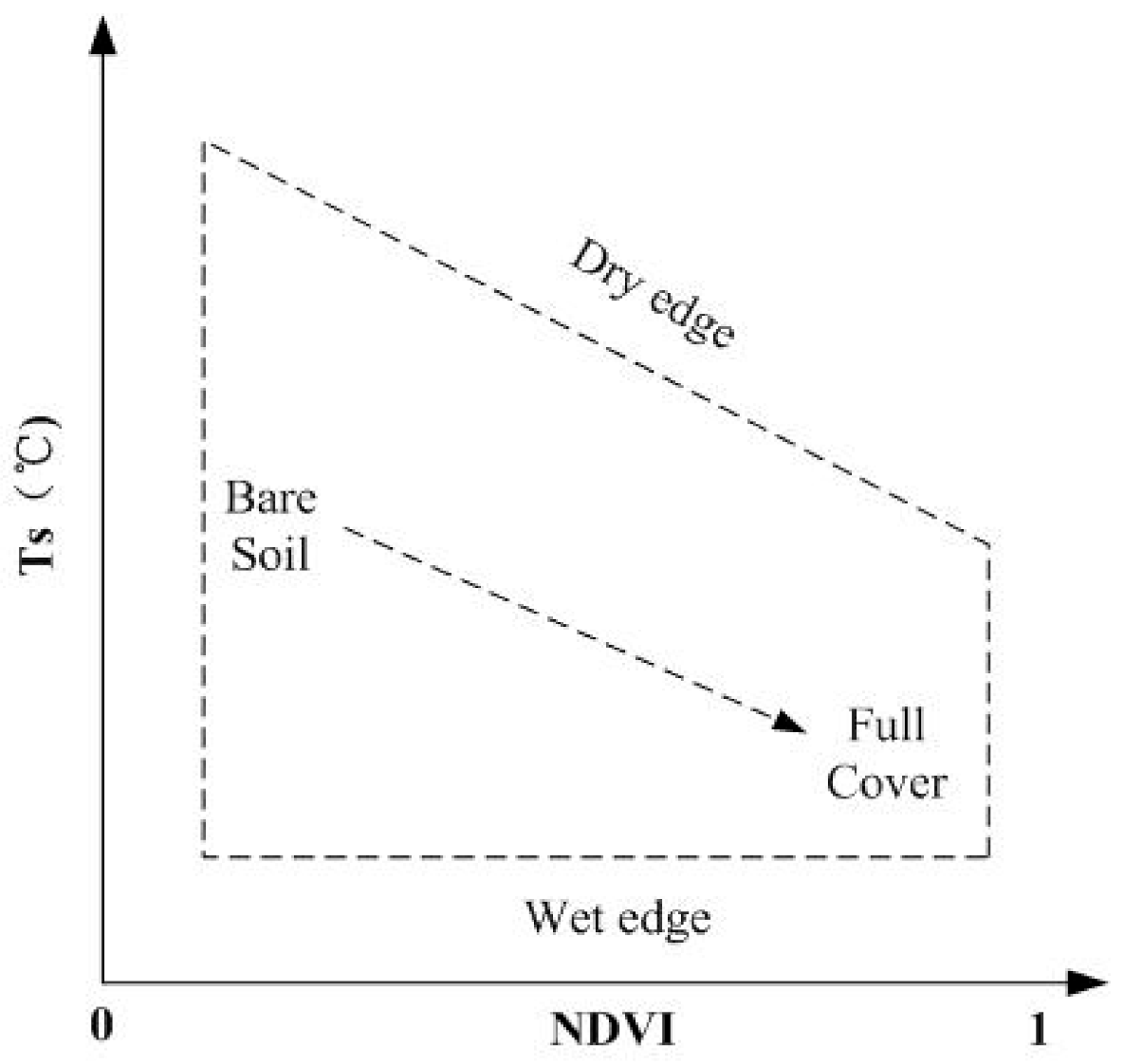
The TVDI model is a dryness index derived from the NDVI–Ts relationship. Figure 3 shows the TVDI trapezoid model that relates SWC to Ts and the NDVI. The left edge of the trapezoid represents bare soil from dry to wet (top-down) conditions. As the ground cover represented by the NDVI increases along the x-axis, the surface temperature (Ts) on the y-axis decreases. For dry conditions, a negative relation is defined by the upper edge, which is the upper limit to surface temperatures for a given surface type [73]. The wet edge of this trapezoid was computed from the mean of all minimum surface temperature (Tmin) values corresponding to 1% NDVI increments (NDVI bin) [27,74]. The TVDI is defined as:
where Ts is the surface temperature derived from the thermal image; Ts,wet is the wet edge y-intercept, i.e., the mean value of minimum Ts for an NDVI value for the model; a is the slope of the dry edge linear regression function; and b is the y-intercept of the dry edge, calculated from linear regression of maximum Ts value for an NDVI value within the model. The NDVI was computed using the reflectance of the red (R) and near-infrared (NIR) bands of the UAS images as:
2.6.2. Theory and Algorithm for the Texture Temperature Vegetation Dryness Index (TTVDI)
Research in soil physics shows that the minimum and maximum SWC (SWCmin and SWCmax, respectively) values depend mainly on the soil texture [75,76]. As in Amazirh et al. [65] and Tomer et al. [77], the SWCmin value could be set to the wilting point, which is related to clay fraction (fclay) by the formula [61]:
and the SWCmax value is calculated from the sand fraction (fsand) as in Cosby et al. [60], which can be set to the SWC at field capacity [65,77]:
SWCmin = 0.15 × fclay
SWCmax = 0.489 − 0.126 × fsand
Based on SWCmin and SWCmax values, SWC at a specific site can be estimated as:
where soil water content percentage (SWCPT) is a percentage parameter based on surface soil temperature, soil temperature on theoretical dry and wet conditions [65,78], which can be estimated as:
SWC = SWCmin + (SWCmax−SWCmin) × SWCPT
After combining Equation (1) to Equation (6), SWCPT can be derived from the trapezoid model and replaced with TVDI:
where Ts is soil surface temperature extracted from the thermal image. Ts, dry and Ts, wet are the highest and lowest soil temperatures in fully dry and wet conditions, respectively. The traditional trapezoid method (Figure 3) was used to estimate the Ts, dry and Ts, wet values based on thermal and multispectral images [79,80].
Combining Equations (1)–(7), soil texture, surface temperature, and the NDVI are incorporated into the texture temperature vegetation dryness index (TTVDI) as:
TTVDI = SWCmin + (SWCmax − SWCmin) × (1-TVDI)
3. Results
3.1. Summary Statistics of Soil Texture and in-situ SWC
The summary statistics of soil texture and in-situ SWC in the 15 cm soil depth are shown in Table 1. Soil sand content in the field ranged from 37.8% to 70.5%. Clay and silt contents ranged from 8.1% to 33.1%, and from 9.0% to 41.2%, respectively. The high variability of soil texture was likely due to the variation in topography over the study area, leading to greater spatial variability in soil water holding capacity. Mean SWC was 18.7%, ranging from 8.0% to 25.9% for the soil samples on 28 April 2019, and mean SWC was 19.6%, ranging from 8.2% to 33.4% for the samples on 19 May 2020.
3.2. Multispectral and Thermal Imagery
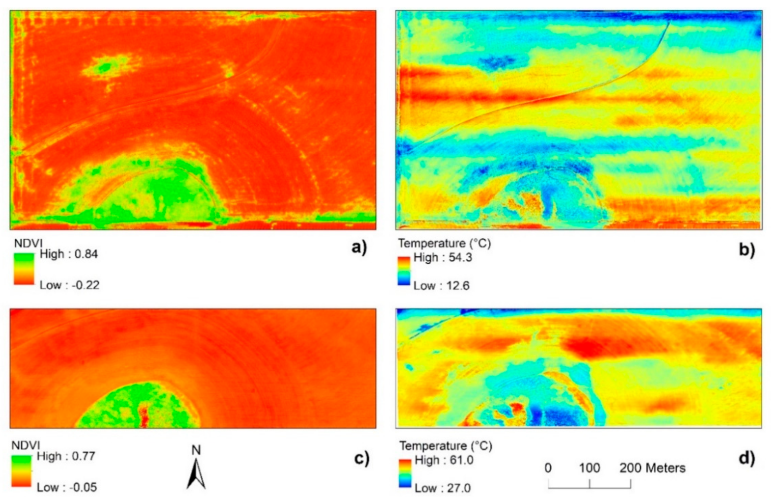
The maps of the NDVI and surface temperature derived from the UAS multispectral and thermal images are shown in Figure 4. Plant cover had an impact on surface temperature (Ts) as low Ts values were associated with high NDVI values. Plant cover was mainly triticum aestivum in the cultivated part or native vegetation in the playa lake. Conversely, the areas with a low NDVI and high Ts indicated bare soil and sparse plant cover.
3.3. SWC Retrieval Using the TVDI and TTVDI
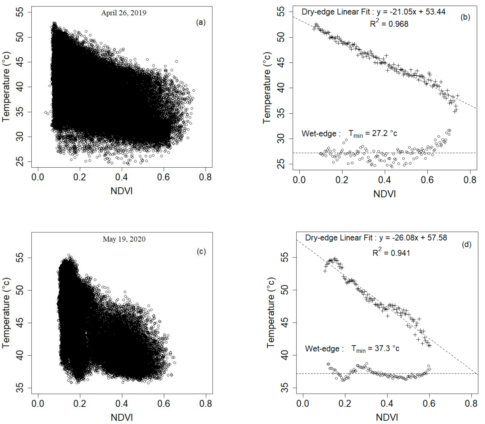
Figure 5 shows the scatter plots of the NDVI against Ts values and their corresponding TVDI parameters derived from the UAS multispectral and thermal images. The TVDI trapezoid models well fit the image data with clear boundaries defined by the wet and dry edges, as indicated by the high R2 values of the linear model for the dry edges (R2 = 0.968 for the images on 28 April 2019, and R2 = 0.941 for the images on 19 May 2020). The wet edge for each date was calculated from the mean of Tmin values. The left edge of the trapezoid model indicated the dry and wet conditions, meaning that temperature changes are mainly explained by changes in water content over the bare soil. The NDVI values increased with vegetation cover.
As shown in Figure 5, compared to the 2019 model, the 2020 model had an overall higher Tmin value due to higher air temperature (Tmin = 37.3 °C in 2020, and Tmin = 27.2 °C in 2019), and fewer high NDVI values greater than 0.6 due to the lower green wheat cover crop in 2020. The high NDVI values for the 2019 model corresponded to the green wheat crop in the south around the playa lake of the field in April, while in 2020, the wheat crop had matured with little green plant material, resulting in low NDVI values in the same area of the field. As shown in Figure 4, the high temperatures corresponding to bare soil appeared in the south part of the field. Therefore, the model differences were mainly in the south part of the field, and the change in the sampling area in 2020 had minimal impact on the model construction.
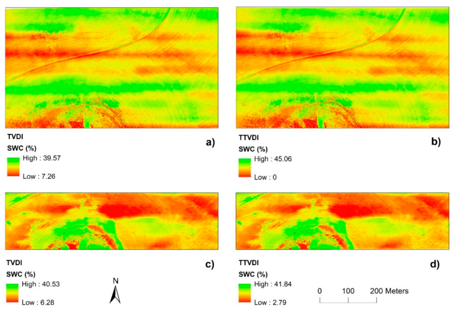
Figure 6 presents the maps of SWC estimated by the TVDI and TTVDI. The SWC calculated by the TVDI was 7.26%~39.57% and 6.28%~40.53% for the 2019 and 2020 surveys, respectively. The SWC calculated by the TTVDI was 0~45.06% for the samples in 2019 and 2.78%~41.84% for those in 2020. An important aspect is that SWC varied significantly across the field, which could be attributed to environmental factors, including topography, vegetation and ground cover, and soil properties, especially soil texture in the 0–15 cm depth.
The summary statistics of SWC retrieved using the TVDI and TTVDI on all sampling points are shown in Table 2. For the sampling point on 28 April 2019, the mean SWCTTVDI was 20.1%, ranging from 8.0% to 29.1%, while the SWCTVDI had a mean of 23.0%, ranging from 3.3% to 44.3%. It indicated the TTVDI performs better than the TVDI. The mean SWCTTVDI was 19.7%, ranging from 8.9% to 35.3%, compared to SWCTVDI with a mean of 20.2%, ranging from 10.3% to 34.3% for the sampling point on 19 May 2020.
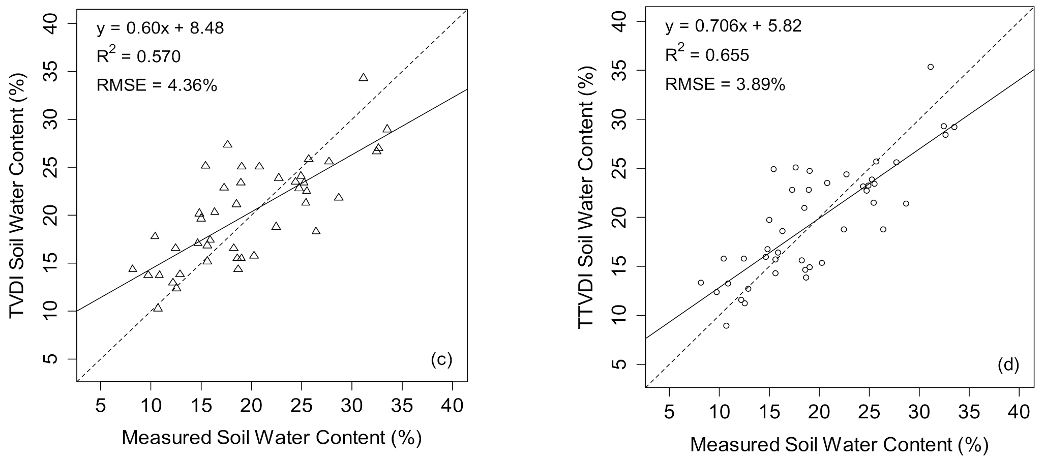
The linear relationships between the in-situ SWC measurements and SWC derived from the TVDI and TTVDI are shown in Figure 7. The TTVDI had a better performance in estimating SWC than the TVDI, as suggested by higher R2 and lower RMSE values for the regression models. The R2 value increased by 14.5%, from 0.588 for the TVDI model to 0.673 for the TTVDI model for the 2019 survey, and it increased by 14.9%, from 0.57 for the TVDI model to 0.655 for the TTVDI model for the 2020 survey. The RMSE decreased by 46.1%, from 5.68% to 3.06% for the 2019 survey, and it decreased by 10.8%, from 4.36% to 3.89 % for the 2020 survey. The SWC values calculated by the TVDI were overestimated in 2019, while they were overestimated when SWC was less than 20%, and underestimated when SWC was greater than 20% for the 2020 survey. The TTVDI presented a systematic overestimation when SWC was less than 20%, and underestimated when SWC was greater than 20% for both the 2019 and 2020 surveys. This may be caused by the difference in thermodynamic characteristics of different soil textures. Some studies have found that thermal diffusivity for sandy soil was small at low SWC and increased with SWC to a maximum value and decreased as SWC continued to increase towards saturation [81,82]. This may cause an overestimation of SWC when retrieved under low water content conditions in sandy soils. On the other hand, Abu-Hamdeh and Reeder (2000) reported that beyond a certain bulk density, higher values of moisture content increased thermal conductivity less rapidly in the case of clayey soils in comparison to sandy soils [83]. So there is no obvious difference in the soil surface temperature when SWC changes within a higher range [84]. That may be the cause of the underestimation of SWC in some clay and high water content areas.
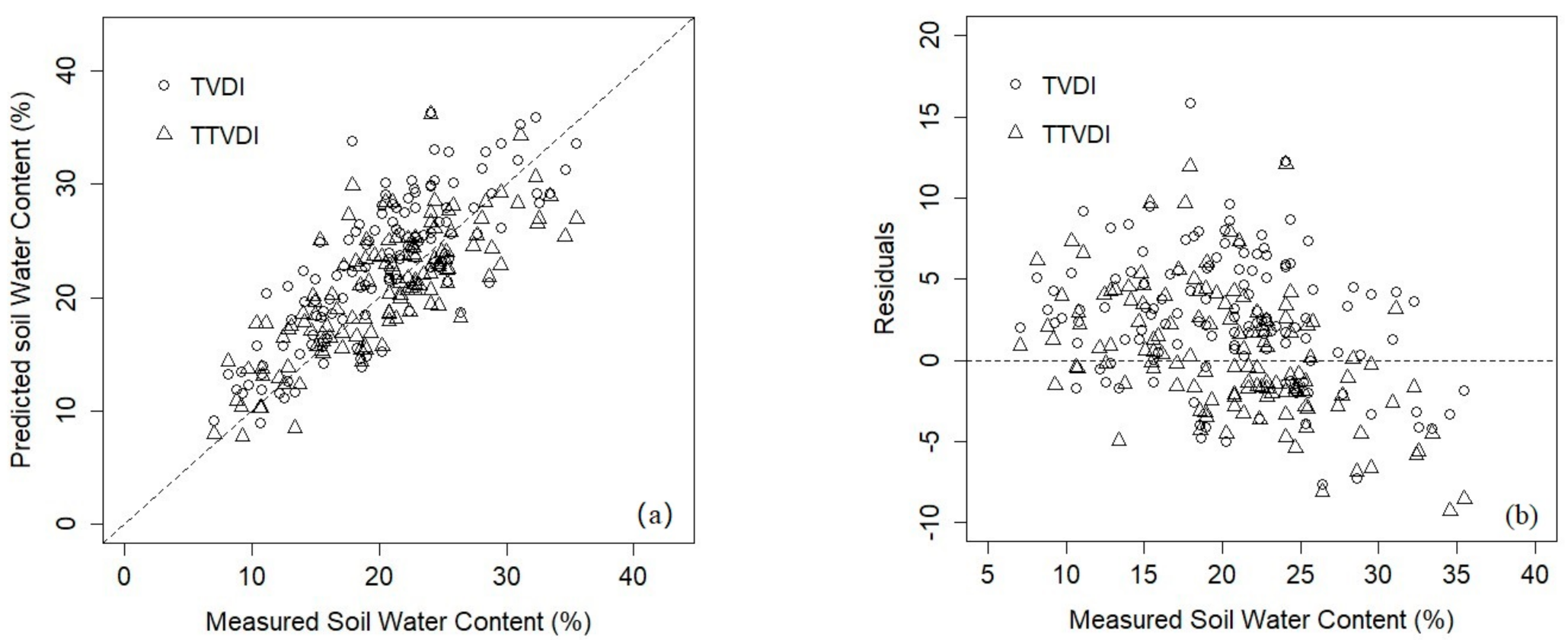
Figure 8 shows the comparison of the TVDI and TTVDI in SWC estimation results for 2019 and 2020. Integrating the relationship of soil texture and SWC, the TTVDI adjusted the calculation results of most points closer to the identity line (1:1 line), which reduced the model residuals. The TTVDI improved the SWC retrieval accuracy; it also increased the prediction errors in some areas. For example, when the SWC was about 30%, the TTVDI underestimated SWC while adjusting the overestimation of the TVDI. This error was likely due to the fact that high-resolution images obtained by UAS are more susceptible to the mixture of vegetation cover, shade, and other surface features (e.g., plant residue, stone), which might affect the model calculation.
4. Discussions
The results of this study showed that the TTVDI generally performed better in estimating SWC as compared to the TVDI for the 2019 and 2020 UAS surveys. The estimation of SWC using the TVDI has a strong dependence on surface temperature. However, the soil temperature is dependent on the interactions between soil thermal properties (e.g., thermal conductivity, thermal diffusivity, volumetric heat capacity, and emissivity characteristics) and SWC, which are also influenced by soil texture [82,83,84,85,86]. Studies have shown that under the same SWC, sandy soils have a higher emissivity and lower thermal resistivity (i.e., reciprocal of thermal conductivity) than clayey soils, resulting in a higher temperature for sandy soils than clayey soils [87,88]. Therefore, SWC based on Ts will be underestimated for sandy soils and overestimated for clayey soils. On the other hand, with the same soil texture, emissivity increases with SWC, especially for sandy soils [89,90]. This may result in underestimation of SWC when SWC increases, particularly for sandy soils with high SWC.
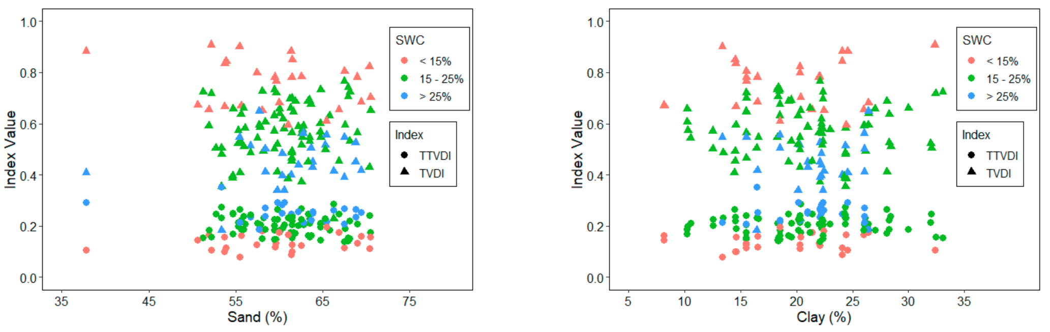
For the same soil sand/clay content, the TTVDI could effectively reduce the estimation error compared to the TVDI. Studies have shown that, in the natural state, the range of SWC mainly depends on the soil porosity, which has a strong relationship with soil sand/clay contents [60,61,75,76]. In this study, soil texture was incorporated in the process of determining the SWCmin and SWCmax. Within this range, SWC has a strong relationship with soil thermal emissivity, which can be monitored dynamically by temperature [89,91]. Figure 9 shows that TTVDI-estimated SWC within a certain range had less variability than that estimated by TVDI. For example, for measured SWC in the range of 15%–25%, the TVDI was between 0.23 and 0.77, while TTVDI ranged from 0.14 to 0.29.
SWC has strong temporal and spatial variability. Research has shown that the application of traditional remote sensing is greatly restricted in the typical agricultural field [27,92]. UAS remote sensing has the advantage of flexibility in acquisition time and resolution, which makes it possible to dynamically monitor SWC at the field scale. The ultimate goal of this new model was to accurately estimate field-level SWC by incorporating soil texture. The derived SWC using the TTVDI had a greater range than the measured SWC, indicating that the soil samples could not represent the whole area with different levels of SWC of the entire field. The extremes of wet (near the playa lake area) and dry areas were not sampled. In addition, soil texture involved in the TTVDI computation for the whole field was interpolated, which could cause errors. Direct inclusion of soil texture information for all pixels would improve the accuracy and efficiency of the TTVDI for SWC estimation. Studies have shown the feasibility of using remote sensing imagery to derive soil texture [93,94,95]. Further research is needed to develop algorithms to derive soil texture from UAS images and integrate that into the TTVDI model. This study was conducted in the early growing season without high ground cover at a dryland field. The model is expected to perform similarly in irrigated fields as the estimation of surface SWC does not depend on dryland or irrigated conditions. However, further research is needed to evaluate the performance of the model under irrigated conditions. In addition, data collection covering the growing season is necessary to assess the applicability of the model under various plant cover conditions.
5. Conclusions
We proposed a new model, the TTVDI, to retrieve surface SWC by incorporating soil texture and Ts and the NDVI derived from high-resolution UAS imagery. The algorithm was based on the relationship between theoretical upper and lower limits of SWC and soil particle sizes. Compared with the TVDI, the R2 of the TTVDI prediction and in situ measurement increased by 14.5% and 14.9%, while the RMSE decreased by 46.1% and 10.8% for the 2019 and 2020 surveys, respectively. The test results show the integration of soil texture data and high spatial resolution images has strong potential in retrieving SWC. However, the relationship established between soil texture and SWC limits in a specific study field, rather than the reference to the empirical model, may further improve the accuracy of the TTVDI model. In the future, incorporating digital soil mapping technology and soil texture spectral characteristics into the model can improve the applicability and accuracy of the model at different scales. At larger scales, the TTVDI model can be constructed to incorporate soil texture information available in soil databases, such as the SSURGO Database, to improve SWC estimation. Further studies are needed to assess the feasibility of incorporating soil databases in the TTVDI for SWC estimation at regional scales.
Author Contributions
Conceptualization, H.G. and W.G.; methodology, H.G. and W.G.; software, H.G.; validation, W.G. and S.D.; formal analysis, H.G.; investigation, H.G., Z.L., W.G. and S.D.; resources, W.G.; data curation, H.G. and Z.L.; writing—original draft preparation, H.G.; writing—review and editing, W.G. and S.D.; visualization, H.G.; supervision, W.G.; project administration, W.G.; funding acquisition, W.G. All authors have read and agreed to the published version of the manuscript.
Funding
This research was funded by Cotton Incorporated and Texas Tech University.
Institutional Review Board Statement
Not applicable for studies not involving humans or animals.
Informed Consent Statement
Not applicable for studies not involving humans.
Data Availability Statement
The data that support the findings of this study are available from the corresponding author upon reasonable request.
Conflicts of Interest
The authors declare no conflict of interest.
References
- Battista, P.; Chiesi, M.; Rapi, B.; Romani, M.; Cantini, C.; Giovannelli, A.; Cocozza, C.; Tognetti, R.; Maselli, F. Integration of ground and multi-resolution satellite data for predicting the water balance of a Mediterranean two-layer agro-ecosystem. Remote Sens. 2016, 8, 731. [Google Scholar] [CrossRef] [Green Version]
- Plaza-Bonilla, D.; Álvaro-Fuentes, J.; Bareche, J.; Pareja-Sánchez, E.; Justes, Éric; Cantero-Martínez, C. No-tillage reduces long-term yield-scaled soil nitrous oxide emissions in rainfed Mediterranean agroecosystems: A field and modelling approach. Agric. Ecosyst. Environ. 2018, 262, 36–47. [Google Scholar] [CrossRef]
- Bond, B.J. Hydrology and ecology meet—and the meeting is good. Hydrol. Process. 2003, 17, 2087–2089. [Google Scholar] [CrossRef]
- Heathman, G.C.; Starks, P.J.; Ahuja, L.R.; Jackson, T.J. Assimilation of surface soil moisture to estimate profile soil water content. J. Hydrol. 2003, 279, 1–17. [Google Scholar] [CrossRef]
- Loik, M.; Breshears, D.D.; Lauenroth, W.K.; Belnap, J. A multi-scale perspective of water pulses in dryland ecosystems: Climatology and ecohydrology of the western USA. Oecologia 2004, 141, 269–281. [Google Scholar] [CrossRef]
- Yu, X.; Guo, X.; Wu, Z. Land surface temperature retrieval from Landsat 8 TIRS—Comparison between radiative transfer equation-based method, split window algorithm and single channel method. Remote Sens. 2014, 6, 9829–9852. [Google Scholar] [CrossRef] [Green Version]
- Zhu, W.; Lv, A.; Jia, S.; Yan, J. A new contextual parameterization of evaporative fraction to reduce the reliance of the Ts—VI triangle method on the dry edge. Remote Sens. 2017, 9, 26. [Google Scholar] [CrossRef] [Green Version]
- Ali, I.; Greifeneder, F.; Stamenkovic, J.; Neumann, M.; Notarnicola, C. Review of machine learning approaches for biomass and soil moisture retrievals from remote sensing data. Remote Sens. 2015, 7, 16398–16421. [Google Scholar] [CrossRef] [Green Version]
- Chew, C.C.; Small, E.E. Soil moisture sensing using spaceborne GNSS reflections: Comparison of CYGNSS reflectivity to SMAP soil moisture. Geophys. Res. Lett. 2018, 45, 4049–4057. [Google Scholar] [CrossRef] [Green Version]
- Lobell, D.B.; Asner, G.P. Moisture Effects on Soil Reflectance. Soil Sci. Soc. Am. J. 2002, 66, 722–727. [Google Scholar] [CrossRef]
- Thorp, K.R.; Thompson, A.L.; Harders, S.J.; French, A.; Ward, R. High-throughput phenotyping of crop water use efficiency via multispectral drone imagery and a daily soil water balance model. Remote Sens. 2018, 10, 1682. [Google Scholar] [CrossRef] [Green Version]
- Chiesi, M.; Battista, P.; Fibbi, L.; Gardin, L.; Pieri, M.; Rapi, B.; Romani, M.; Sabatini, F.; Maselli, F. Spatio-temporal fusion of NDVI data for simulating soil water content in heterogeneous Mediterranean areas. Eur. J. Remote Sens. 2018, 52, 88–95. [Google Scholar] [CrossRef] [Green Version]
- Sadeghi, M.; Babaeian, E.; Tuller, M.; Jones, S.B. The optical trapezoid model: A novel approach to remote sensing of soil moisture applied to Sentinel-2 and Landsat-8 observations. Remote Sens. Environ. 2017, 198, 52–68. [Google Scholar] [CrossRef] [Green Version]
- Fang, L.; Hain, C.R.; Zhan, X.; Anderson, M. An inter-comparison of soil moisture data products from satellite remote sensing and a land surface model. Int. J. Appl. Earth Obs. Geoinf. 2016, 48, 37–50. [Google Scholar] [CrossRef]
- He, M.; Kimball, J.S.; Running, S.; Ballantyne, A.; Guan, K.; Huemmrich, F. Satellite detection of soil moisture related water stress impacts on ecosystem productivity using the MODIS-based photochemical reflectance index. Remote Sens. Environ. 2016, 186, 173–183. [Google Scholar] [CrossRef] [Green Version]
- Nemani, R.; Pierce, L.; Running, S.; Goward, S. Developing satellite-derived estimates of surface moisture status. J. Appl. Meteorol. 1993, 32, 548–557. [Google Scholar] [CrossRef] [Green Version]
- Sadeghi, M.; Jones, S.B.; Philpot, W.D. A linear physically-based model for remote sensing of soil moisture using short wave infrared bands. Remote Sens. Environ. 2015, 164, 66–76. [Google Scholar] [CrossRef]
- Aubert, M.; Baghdadi, N.; Zribi, M.; Douaoui, A.; Loumagne, C.; Baup, F.; El Hajj, M.; Garrigues, S. Analysis of TerraSAR-X data sensitivity to bare soil moisture, roughness, composition and soil crust. Remote Sens. Environ. 2011, 115, 1801–1810. [Google Scholar] [CrossRef] [Green Version]
- Dube, T.; Onisimo, M.; Sibanda, M.; Shoko, C.; Chemura, A. Evaluating the influence of the Red Edge band from RapidEye sensor in quantifying leaf area index for hydrological applications specifically focussing on plant canopy interception. Phys. Chem. Earth Parts A/B/C 2017, 100, 73–80. [Google Scholar] [CrossRef]
- Du, L.; Song, N.; Liu, K.; Hou, J.; Hu, Y.; Zhu, Y.; Wang, X.; Wang, L.; Guo, Y. Comparison of two simulation methods of the Temperature Vegetation Dryness Index (TVDI) for drought monitoring in semi-arid regions of China. Remote Sens. 2017, 9, 177. [Google Scholar] [CrossRef] [Green Version]
- Gao, Z.; Gao, W.; Chang, N.-B. Integrating temperature vegetation dryness index (TVDI) and regional water stress index (RWSI) for drought assessment with the aid of LANDSAT TM/ETM+ images. Int. J. Appl. Earth Obs. Geoinf. 2011, 13, 495–503. [Google Scholar] [CrossRef]
- Park, S.; Feddema, J.J.; Egbert, S.L. Impacts of hydrologic soil properties on drought detection with MODIS thermal data. Remote Sens. Environ. 2004, 89, 53–62. [Google Scholar] [CrossRef]
- Rahimzadeh-Bajgiran, P.; Berg, A.A.; Champagne, C.; Omasa, K. Estimation of soil moisture using optical/thermal infrared remote sensing in the Canadian Prairies. ISPRS J. Photogramm. Remote Sens. 2013, 83, 94–103. [Google Scholar] [CrossRef]
- Amani, M.; Salehi, B.; Mahdavi, S.; Masjedi, A.; Dehnavi, S. Temperature-Vegetation-soil Moisture Dryness Index (TVMDI). Remote Sens. Environ. 2017, 197, 1–14. [Google Scholar] [CrossRef]
- Patel, N.; Anapashsha, R.; Kumar, S.; Saha, S.K.; Dadhwal, V.K. Assessing potential of MODIS derived temperature/vegetation condition index (TVDI) to infer soil moisture status. Int. J. Remote Sens. 2008, 30, 23–39. [Google Scholar] [CrossRef]
- Wang, C.; Qi, S.; Niu, Z.; Wang, J. Evaluating soil moisture status in China using the temperature–vegetation dryness index (TVDI). Can. J. Remote Sens. 2004, 30, 671–679. [Google Scholar] [CrossRef]
- Wigmore, O.; Mark, B.; McKenzie, J.; Baraer, M.; Lautz, L. Sub-metre mapping of surface soil moisture in proglacial valleys of the tropical Andes using a multispectral unmanned aerial vehicle. Remote Sens. Environ. 2019, 222, 104–118. [Google Scholar] [CrossRef]
- Yan, H.; Zhou, G.; Yang, F.; Lu, X. DEM correction to the TVDI method on drought monitoring in karst areas. Int. J. Remote Sens. 2019, 40, 2166–2189. [Google Scholar] [CrossRef]
- Zhang, T.; Cai, G.; Liu, S.; Puppala, A.J. Investigation on thermal characteristics and prediction models of soils. Int. J. Heat Mass Transf. 2017, 106, 1074–1086. [Google Scholar] [CrossRef]
- Leng, P.; Song, X.; Duan, S.-B.; Li, Z.-L. A practical algorithm for estimating surface soil moisture using combined optical and thermal infrared data. Int. J. Appl. Earth Obs. Geoinf. 2016, 52, 338–348. [Google Scholar] [CrossRef]
- Kaplan, G.; Avdan, U. Evaluating the utilization of the red edge and radar bands from sentinel sensors for wetland classification. Catena 2019, 178, 109–119. [Google Scholar] [CrossRef]
- Nutini, F.; Stroppiana, D.; Busetto, L.; Bellingeri, D.; Corbari, C.; Mancini, M.; Zini, E.; Brivio, P.A.; Boschetti, M. A weekly indicator of surface moisture status from satellite data for operational monitoring of crop conditions. Sensors 2017, 17, 1338. [Google Scholar] [CrossRef] [PubMed] [Green Version]
- Shwetha, H.R.; Kumar, D.N. Estimation of daily vegetation coefficients using MODIS data for clear and cloudy sky conditions. Int. J. Remote Sens. 2018, 39, 3776–3800. [Google Scholar] [CrossRef]
- Holzman, M.; Rivas, R.; Piccolo, M.C. Estimating soil moisture and the relationship with crop yield using surface temperature and vegetation index. Int. J. Appl. Earth Obs. Geoinf. 2014, 28, 181–192. [Google Scholar] [CrossRef]
- Rahimzadeh-Bajgiran, P.; Omasa, K.; Shimizu, Y. Comparative evaluation of the Vegetation Dryness Index (VDI), the Temperature Vegetation Dryness Index (TVDI) and the improved TVDI (iTVDI) for water stress detection in semi-arid regions of Iran. ISPRS J. Photogramm. Remote Sens. 2012, 68, 1–12. [Google Scholar] [CrossRef]
- Zhao, J.; Zhang, X.; Bao, H. Soil moisture retrieval from remote sensing data in arid areas using a multiple models strategy. In Advances in Intelligent and Soft Computing; Springer: Berlin/Heidelberg, Germany, 2011; pp. 635–643. [Google Scholar]
- Brisco, B.; Brown, R.; Hirose, T.; McNairn, H.; Staenz, K. Precision agriculture and the role of remote sensing: A review. Can. J. Remote Sens. 1998, 24, 315–327. [Google Scholar] [CrossRef]
- Gago, J.; Douthe, C.; Coopman, R.; Gallego, P.; Ribascarbo, M.; Flexas, J.; Escalona, J.M.; Medrano, H. UAVs challenge to assess water stress for sustainable agriculture. Agric. Water Manag. 2015, 153, 9–19. [Google Scholar] [CrossRef]
- Aasen, H.; Honkavaara, E.; Lucieer, A.; Zarco-Tejada, P.J. Quantitative remote sensing at ultra-high resolution with UAV spectroscopy: A review of sensor technology, measurement procedures, and data correction workflows. Remote Sens. 2018, 10, 1091. [Google Scholar] [CrossRef] [Green Version]
- Santesteban, L.; Di Gennaro, S.; Herrero-Langreo, A.; Miranda, C.; Royo, J.; Matese, A. High-resolution UAV-based thermal imaging to estimate the instantaneous and seasonal variability of plant water status within a vineyard. Agric. Water Manag. 2017, 183, 49–59. [Google Scholar] [CrossRef]
- Holah, N.; Baghdadi, N.; Zribi, M.; Bruand, A.; King, C. Potential of ASAR/ENVISAT for the characterization of soil surface parameters over bare agricultural fields. Remote Sens. Environ. 2005, 96, 78–86. [Google Scholar] [CrossRef] [Green Version]
- Mogili, U.R.; Deepak, B.B.V.L. Review on application of drone systems in precision agriculture. Procedia Comput. Sci. 2018, 133, 502–509. [Google Scholar] [CrossRef]
- Hassan-Esfahani, L.; Torres-Rua, A.; Jensen, A.M.; McKee, M. Assessment of surface soil moisture using high-resolution multi-spectral imagery and artificial neural networks. Remote Sens. 2015, 7, 2627–2646. [Google Scholar] [CrossRef] [Green Version]
- Gnädinger, F.; Schmidhalter, U. Digital Counts of Maize Plants by Unmanned Aerial Vehicles (UAVs). Remote Sens. 2017, 9, 544. [Google Scholar] [CrossRef] [Green Version]
- Wu, J.; Yang, G.; Yang, X.; Xu, B.; Han, L.; Zhu, Y. Automatic counting of in situ rice seedlings from UAV images based on a deep fully convolutional neural network. Remote Sens. 2019, 11, 691. [Google Scholar] [CrossRef] [Green Version]
- Malambo, L.; Popescu, S.; Murray, S.; Putman, E.; Pugh, N.; Horne, D.; Richardson, G.; Sheridan, R.; Rooney, W.; Avant, R.; et al. Multitemporal field-based plant height estimation using 3D point clouds generated from small unmanned aerial systems high-resolution imagery. Int. J. Appl. Earth Obs. Geoinf. 2018, 64, 31–42. [Google Scholar] [CrossRef]
- Osco, L.P.; Ramos, A.P.M.; Moriya, Érika, A.S.; De Souza, M.; Junior, J.M.; Matsubara, E.T.; Imai, N.N.; Creste, J.E. Improvement of leaf nitrogen content inference in Valencia-orange trees applying spectral analysis algorithms in UAV mounted-sensor images. Int. J. Appl. Earth Obs. Geoinf. 2019, 83, 101907. [Google Scholar] [CrossRef]
- Walshe, D.; McInerney, D.; Van De Kerchove, R.; Goyens, C.; Balaji, P.; Byrne, K.A. Detecting nutrient deficiency in spruce forests using multispectral satellite imagery. Int. J. Appl. Earth Obs. Geoinf. 2020, 86, 101975. [Google Scholar] [CrossRef]
- Ballesteros, R.; Ortega, J.F.; Hernandez, D.; Moreno, M.A. Onion biomass monitoring using UAV-based RGB imaging. Precis. Agric. 2018, 19, 840–857. [Google Scholar] [CrossRef]
- Yao, X.; Wang, N.; Liu, Y.; Cheng, T.; Tian, Y.; Chen, Q.; Zhu, Y. Estimation of wheat LAI at middle to high levels using unmanned aerial vehicle narrowband multispectral imagery. Remote Sens. 2017, 9, 1304. [Google Scholar] [CrossRef] [Green Version]
- Sanches, G.M.; Duft, D.G.; Kölln, O.T.; Luciano, A.C.D.S.; De Castro, S.G.Q.; Okuno, F.M.; Franco, H.C.J. The potential for RGB images obtained using unmanned aerial vehicle to assess and predict yield in sugarcane fields. Int. J. Remote Sens. 2018, 39, 5402–5414. [Google Scholar] [CrossRef]
- Schut, A.G.T.; Traore, P.C.S.; Blaes, X.; De By, R.A. Assessing yield and fertilizer response in heterogeneous smallholder fields with UAVs and satellites. Field Crop. Res. 2018, 221, 98–107. [Google Scholar] [CrossRef]
- Acevo-Herrera, R.; Aguasca, A.; Bosch-Lluis, X.; Camps, A.; Martínez-Fernández, J.; Sanchez, N.; Pérez-Gutiérrez, C. Design and first results of an UAV-norne L-Band radiometer for multiple monitoring purposes. Remote Sens. 2010, 2, 1662–1679. [Google Scholar] [CrossRef] [Green Version]
- Hsu, W.-L.; Chang, K.-T. Cross-estimation of soil moisture using thermal infrared images with different resolutions. Sens. Mater. 2019, 31, 387. [Google Scholar] [CrossRef]
- Raihan, A. Surface Soil Moisture Estimation Using Unmanned Aerial System and Satellite Images. Master’s Thesis, Texas Tech University, Lubbock, TX, USA, 2018. [Google Scholar]
- Gorrab, A.; Zribi, M.; Baghdadi, N.; Mougenot, B.; Fanise, P.; Lili-Chabaane, Z. Retrieval of both soil moisture and texture using terraSAR-X images. Remote Sens. 2015, 7, 10098–10116. [Google Scholar] [CrossRef] [Green Version]
- Baroni, G.; Ortuani, B.; Facchi, A.; Gandolfi, C. The role of vegetation and soil properties on the spatio-temporal variability of the surface soil moisture in a maize-cropped field. J. Hydrol. 2013, 489, 148–159. [Google Scholar] [CrossRef]
- Dari, J.; Morbidelli, R.; Saltalippi, C.; Massari, C.; Brocca, L. Spatial-temporal variability of soil moisture: Addressing the monitoring at the catchment scale. J. Hydrol. 2019, 570, 436–444. [Google Scholar] [CrossRef]
- Lu, Y.; Horton, R.; Zhang, X.; Ren, T. Accounting for soil porosity improves a thermal inertia model for estimating surface soil water content. Remote Sens. Environ. 2018, 212, 79–89. [Google Scholar] [CrossRef]
- Cosby, B.J.; Hornberger, G.M.; Clapp, R.B.; Ginn, T.R. A statistical exploration of the relationships of soil moisture characteristics to the physical properties of soils. Water Resour. Res. 1984, 20, 682–690. [Google Scholar] [CrossRef] [Green Version]
- Brisson, N.; Perrier, A. A semiempirical model of bare soil evaporation for crop simulation models. Water Resour. Res. 1991, 27, 719–727. [Google Scholar] [CrossRef]
- Escadafal, R. Soil spectral properties and their relationships with environmental parameters—Examples from arid regions. In Eurocourses: Remote Sensing; Springer: Berlin/Heidelberg, Germany, 1994; pp. 71–87. [Google Scholar]
- Gholizadeh, A.; Žižala, D.; Saberioon, M.; Borůvka, L. Soil organic carbon and texture retrieving and mapping using proximal, airborne and Sentinel-2 spectral imaging. Remote Sens. Environ. 2018, 218, 89–103. [Google Scholar] [CrossRef]
- Whiting, M.L.; Li, L.; Ustin, S.L. Predicting water content using Gaussian model on soil spectra. Remote Sens. Environ. 2004, 89, 535–552. [Google Scholar] [CrossRef]
- Amazirh, A.; Merlin, O.; Er-Raki, S.; Gao, Q.; Rivalland, V.; Malbeteau, Y.; Khabba, S.; Escorihuela, M.J. Retrieving surface soil moisture at high spatio-temporal resolution from a synergy between Sentinel-1 radar and Landsat thermal data: A study case over bare soil. Remote Sens. Environ. 2018, 211, 321–337. [Google Scholar] [CrossRef]
- United States Climate Data (USCD). Lubbock, Texas Climate Data. Available online: https://www.usclimatedata.com/climate/lubbock/texas/united-states/ustx2745 (accessed on 11 August 2020).
- Long, D.; Rehm, P.; Ferguson, S. Benefits and challenges of using unmanned aerial systems in the monitoring of electrical distribution systems. Electr. J. 2018, 31, 26–32. [Google Scholar] [CrossRef]
- Dugdale, S.J.; Kelleher, C.; Malcolm, I.A.; Caldwell, S.; Hannah, D.M. Assessing the potential of drone-based thermal infrared imagery for quantifying river temperature heterogeneity. Hydrol. Process. 2019, 33, 1152–1163. [Google Scholar] [CrossRef]
- Sharma, L.K.; Bu, H.; Denton, A.; Franzen, D.W. Active-optical sensors using red NDVI compared to red edge NDVI for prediction of corn grain yield in North Dakota, U.S.A. Sensors 2015, 15, 27832–27853. [Google Scholar] [CrossRef]
- MicaSense. Downwelling Light Sensor (DLS) Integration Guide and User Manual. Available online: https://support.micasense.com/hc/en-us/articles/218233618-Downwelling-Light-Sensor-DLS-Integration-Guide-PDF-Download (accessed on 17 December 2020).
- Honkavaara, E.; Eskelinen, M.A.; Pölönen, I.; Saari, H.; Ojanen, H.; Mannila, R.; Holmlund, C.; Hakala, T.; Litkey, P.; Rosnell, T.; et al. Remote sensing of 3-D geometry and surface moisture of a peat production area using hyperspectral frame cameras in visible to short-wave infrared spectral ranges onboard a small unmanned airborne vehicle (UAV). IEEE Trans. Geosci. Remote Sens. 2016, 54, 5440–5454. [Google Scholar] [CrossRef] [Green Version]
- Klute, A. Methods of Soil Analysis. Part 1, 2nd ed.; American Society of Agronomy: Madison, WI, USA, 1986; pp. 383–411. [Google Scholar]
- Liu, Y.; Yue, H. The temperature vegetation dryness index (TVDI) based on Bi-Parabolic NDVI-Ts space and gradient-based structural similarity (GSSIM) for long-term drought assessment across Shaanxi Province, China (2000–2016). Remote Sens. 2018, 10, 959. [Google Scholar] [CrossRef] [Green Version]
- Ezzine, H.; Bouziane, A.; Ouazar, D. Seasonal comparisons of meteorological and agricultural drought indices in Morocco using open short time-series data. Int. J. Appl. Earth Obs. Geoinf. 2014, 26, 36–48. [Google Scholar] [CrossRef]
- Dexter, A.; Bird, N. Methods for predicting the optimum and the range of soil water contents for tillage based on the water retention curve. Soil Tillage Res. 2001, 57, 203–212. [Google Scholar] [CrossRef]
- Carsel, R.F.; Parrish, R.S. Developing joint probability distributions of soil water retention characteristics. Water Resour. Res. 1988, 24, 755–769. [Google Scholar] [CrossRef] [Green Version]
- Tomer, S.K.; Al Bitar, A.; Muddu, S.; Zribi, M.; Bandyopadhyay, S.; Sreelash, K.; Sharma, A.; Corgne, S.; Kerr, Y. Retrieval and multi-scale validation of soil moisture from multi-temporal SAR data in a semi-arid tropical region. Remote Sens. 2015, 7, 8128–8153. [Google Scholar] [CrossRef] [Green Version]
- Lakshmi, V.; Jackson, T.J.; Zehrfuhs, D. Soil moisture-temperature relationships: Results from two field experiments. Hydrol. Process. 2003, 17, 3041–3057. [Google Scholar] [CrossRef]
- Zhu, W.; Zhu, W.; Lv, A. A time domain solution of the modified temperature vegetation dryness index (MTVDI) for continuous soil moisture monitoring. Remote Sens. Environ. 2017, 200, 1–17. [Google Scholar] [CrossRef]
- Shafian, S.; Maas, S.J. Improvement of the trapezoid method using raw Landsat image digital count data for soil moisture estimation in the Texas (USA) high plains. Sensors 2015, 15, 1925–1944. [Google Scholar] [CrossRef] [Green Version]
- Abu-Hamdeh, N.H. Thermal properties of soils as affected by density and water content. Biosyst. Eng. 2003, 86, 97–102. [Google Scholar] [CrossRef]
- Nikoosokhan, S.; Nowamooz, H.; Chazallon, C. Effect of dry density, soil texture and time-spatial variable water content on the soil thermal conductivity. Géoméch. Geoengin. 2015, 11, 149–158. [Google Scholar] [CrossRef]
- Abu-Hamdeh, N.H.; Reeder, R.C. Soil thermal conductivity effects of density, moisture, salt concentration, and organic matter. Soil Sci. Soc. Am. J. 2000, 64, 1285–1290. [Google Scholar] [CrossRef]
- Van De Griend, A.A.; Camillo, P.J.; Gurney, R.J. Discrimination of soil physical parameters, thermal inertia, and soil moisture from diurnal surface temperature fluctuations. Water Resour. Res. 1985, 21, 997–1009. [Google Scholar] [CrossRef]
- Huang, P.M.; Li, Y.; Sumner, M.E. Handbook of Soil Sciences: Properties and Processes, 2nd ed.; CRC Press: Boca Raton, FL, USA, 2011; pp. 1440–1445. [Google Scholar]
- Barry-Macaulay, D.; Bouazza, A.; Wang, B.; Singh, R. Evaluation of soil thermal conductivity models. Can. Geotech. J. 2015, 52, 1892–1900. [Google Scholar] [CrossRef]
- Salisbury, J.W.; D’Aria, D.M. Infrared (8–14 μm) remote sensing of soil particle size. Remote Sens. Environ. 1992, 42, 157–165. [Google Scholar] [CrossRef]
- Singh, D.N.; Devid, K. Generalized relationships for estimating soil thermal resistivity. Exp. Therm. Fluid Sci. 2000, 22, 133–143. [Google Scholar] [CrossRef]
- Miralles, V.C.; Valor, E.; Boluda, R.; Caselles, V.; Coll, C. Influence of soil water content on the thermal infrared emissivity of bare soils: Implication for land surface temperature determination. J. Geophys. Res. Space Phys. 2007, 112. [Google Scholar] [CrossRef] [Green Version]
- Mira, M.; Valor, E.; Caselles, V.; Rubio, E.; Coll, C.; Galve, J.M.; Niclos, R.; Sanchez, J.M.; Boluda, R. Soil moisture effect on thermal infrared (8–13 μm) emissivity. IEEE Trans. Geosci. Remote Sens. 2010, 48, 2251–2260. [Google Scholar] [CrossRef]
- Sanchez, J.M.; French, A.N.; Mira, M.; Hunsaker, D.; Thorp, K.R.; Valor, E.; Caselles, V. Thermal infrared emissivity dependence on soil moisture in field conditions. IEEE Trans. Geosci. Remote Sens. 2011, 49, 4652–4659. [Google Scholar] [CrossRef]
- Zhang, L.; Jiao, W.; Zhang, H.; Huang, C.; Tong, Q. Studying drought phenomena in the Continental United States in 2011 and 2012 using various drought indices. Remote Sens. Environ. 2017, 190, 96–106. [Google Scholar] [CrossRef]
- Castaldi, F.; Palombo, A.; Santini, F.; Pascucci, S.; Pignatti, S.; Casa, R. Evaluation of the potential of the current and forthcoming multispectral and hyperspectral imagers to estimate soil texture and organic carbon. Remote Sens. Environ. 2016, 179, 54–65. [Google Scholar] [CrossRef]
- Liao, K.; Xu, S.; Wu, J.; Zhu, Q. Spatial estimation of surface soil texture using remote sensing data. Soil Sci. Plant Nutr. 2013, 59, 488–500. [Google Scholar] [CrossRef]
- Shahriari, M.; Delbari, M.; Afrasiab, P.; Pahlavan-Rad, M.R. Predicting regional spatial distribution of soil texture in floodplains using remote sensing data: A case of southeastern Iran. Catena 2019, 182, 104149. [Google Scholar] [CrossRef]
Figure 1.
Study field with soil sampling locations and soil map units in Garza County, Texas. AcA: Acuff loam, 0 to 1% slopes (fine-loamy, mixed, superactive, thermic Aridic Paleustolls); AmB: Amarillo fine sandy loam, 1 to 3% slopes (fine-loamy, mixed, superactive, thermic Aridic Paleustalfs); Ra: Randall clay, 0 to 1% slopes, occasionally ponded (fine, smectitic, thermic Ustic Epiaquerts); OIA: Olton loam, 0 to 1% slopes (fine-loamy, mixed, superactive, thermic Aridic Paleustolls); and AcB: Acuff loam, 1 to 3% slopes (fine-loamy, mixed, superactive, thermic Aridic Paleustolls).

Figure 2.
UAS platform and sensors applied in acquiring multispectral and thermal images for retrieval of surface SWC. (A) DJI Matrice 600 Pro UAS platform; (B) MicaSense RedEdge multispectral sensor; and (C) DJI Zenmuse XT thermal sensor.
Figure 2.
UAS platform and sensors applied in acquiring multispectral and thermal images for retrieval of surface SWC. (A) DJI Matrice 600 Pro UAS platform; (B) MicaSense RedEdge multispectral sensor; and (C) DJI Zenmuse XT thermal sensor.

Figure 3.
The temperature vegetation dryness index (TVDI) model showing the relationship between the NDVI and surface temperature Ts [16].
Figure 3.
The temperature vegetation dryness index (TVDI) model showing the relationship between the NDVI and surface temperature Ts [16].

Figure 4.
The NDVI and temperature are derived from UAS multispectral and thermal infrared images for an agricultural field in Garza County, Texas. (a) and (b) were derived from images acquired on 28 April 2019; (c) and (d) were derived from images acquired on 19 May 2020.
Figure 4.
The NDVI and temperature are derived from UAS multispectral and thermal infrared images for an agricultural field in Garza County, Texas. (a) and (b) were derived from images acquired on 28 April 2019; (c) and (d) were derived from images acquired on 19 May 2020.

Figure 5.
Scatterplots and boundary condition functions of dry and wet edges for the TVDI trapezoid models consisting of the NDVI and Ts values derived from UAS images for an agricultural field in Garza County, Texas.
Figure 5.
Scatterplots and boundary condition functions of dry and wet edges for the TVDI trapezoid models consisting of the NDVI and Ts values derived from UAS images for an agricultural field in Garza County, Texas.

Figure 6.
SWC distribution derived from the TVDI and TTVDI models. (a) and (b) are the SWC estimation results for the UAS survey on 28 April 2019; (c) and (d) are the SWC estimation results for the UAS survey on 19 May 2020.
Figure 6.
SWC distribution derived from the TVDI and TTVDI models. (a) and (b) are the SWC estimation results for the UAS survey on 28 April 2019; (c) and (d) are the SWC estimation results for the UAS survey on 19 May 2020.

Figure 7.
SWC estimation using the TVDI and TTVDI compared to in-situ SWC measurements for a field in Garza County, Texas. (a) and (b) for the UAS survey on 28 April 2019; (c) and (d) for the UAS survey on 19 May 2020.
Figure 7.
SWC estimation using the TVDI and TTVDI compared to in-situ SWC measurements for a field in Garza County, Texas. (a) and (b) for the UAS survey on 28 April 2019; (c) and (d) for the UAS survey on 19 May 2020.


Figure 8.
Comparison of the TVDI and TTVDI in estimating SWC using UAS multispectral and thermal images in 2019 and 2020. (a) SWC retrieval results by the TVDI and TTVDI vs. SWC measurements. (b) Estimation residuals of the TVDI and TTVDI.
Figure 8.
Comparison of the TVDI and TTVDI in estimating SWC using UAS multispectral and thermal images in 2019 and 2020. (a) SWC retrieval results by the TVDI and TTVDI vs. SWC measurements. (b) Estimation residuals of the TVDI and TTVDI.

Figure 9.
Comparison of TVDI and TTVDI values in estimating surface SWC as a function of soil sand and clay contents.
Figure 9.
Comparison of TVDI and TTVDI values in estimating surface SWC as a function of soil sand and clay contents.


Table 1.
Summary statistics of soil texture and SWC of 84 soil samples collected on 28 April 2019, and 44 samples on 19 May 2020, from a field near Slaton, Texas.
Table 1.
Summary statistics of soil texture and SWC of 84 soil samples collected on 28 April 2019, and 44 samples on 19 May 2020, from a field near Slaton, Texas.
| Soil Property | Minimum | Maximum | Mean | Std. Deviation | Median |
|---|---|---|---|---|---|
| Clay (%) | 8.1 | 33.1 | 20.9 | 5.8 | 21.3 |
| Silt (%) | 9.0 | 41.2 | 19.0 | 7.2 | 17.0 |
| Sand (%) | 37.8 | 70.5 | 60.1 | 5.5 | 60.4 |
| SWC (%) (2019) | 8.0 | 25.9 | 18.7 | 4.7 | 21.4 |
| SWC (%) (2020) | 8.2 | 33.4 | 19.6 | 6.7 | 18.6 |
Table 2.
Summary statistics of SWC retrieved using the TVDI and TTVDI on 84 sampling points on 28 April 2019, and 44 sampling points on 19 May 2020.
Table 2.
Summary statistics of SWC retrieved using the TVDI and TTVDI on 84 sampling points on 28 April 2019, and 44 sampling points on 19 May 2020.
| Date | SWC (%) | Minimum | Maximum | Mean | Std. Deviation | Median |
|---|---|---|---|---|---|---|
| 28 April 2019 | SWCMeasured | 8.0 | 25.9 | 18.7 | 4.7 | 21.4 |
| SWCTVDI | 3.3 | 44.3 | 23.0 | 8.2 | 23.3 | |
| SWCTTVDI | 8.0 | 29.1 | 20.1 | 4.6 | 20.7 | |
| May 17, 2020 | SWCMeasured | 8.2 | 33.4 | 19.6 | 6.7 | 18.6 |
| SWCTVDI | 10.3 | 34.3 | 20.2 | 5.3 | 20.2 | |
| SWCTTVDI | 8.9 | 35.3 | 19.7 | 5.8 | 19.2 |
Publisher’s Note: MDPI stays neutral with regard to jurisdictional claims in published maps and institutional affiliations. |
© 2021 by the authors. Licensee MDPI, Basel, Switzerland. This article is an open access article distributed under the terms and conditions of the Creative Commons Attribution (CC BY) license (http://creativecommons.org/licenses/by/4.0/).
Share and Cite
MDPI and ACS Style
Gu, H.; Lin, Z.; Guo, W.; Deb, S. Retrieving Surface Soil Water Content Using a Soil Texture Adjusted Vegetation Index and Unmanned Aerial System Images. Remote Sens. 2021, 13, 145. https://0-doi-org.brum.beds.ac.uk/10.3390/rs13010145
AMA Style
Gu H, Lin Z, Guo W, Deb S. Retrieving Surface Soil Water Content Using a Soil Texture Adjusted Vegetation Index and Unmanned Aerial System Images. Remote Sensing. 2021; 13(1):145. https://0-doi-org.brum.beds.ac.uk/10.3390/rs13010145
Chicago/Turabian StyleGu, Haibin, Zhe Lin, Wenxuan Guo, and Sanjit Deb. 2021. "Retrieving Surface Soil Water Content Using a Soil Texture Adjusted Vegetation Index and Unmanned Aerial System Images" Remote Sensing 13, no. 1: 145. https://0-doi-org.brum.beds.ac.uk/10.3390/rs13010145
Note that from the first issue of 2016, this journal uses article numbers instead of page numbers. See further details here.