Intra-Annual Sentinel-2 Time-Series Supporting Grassland Habitat Discrimination

 ,
,  , ,
, ,  and
and
Abstract
:
1. Introduction
2. Materials and Methods
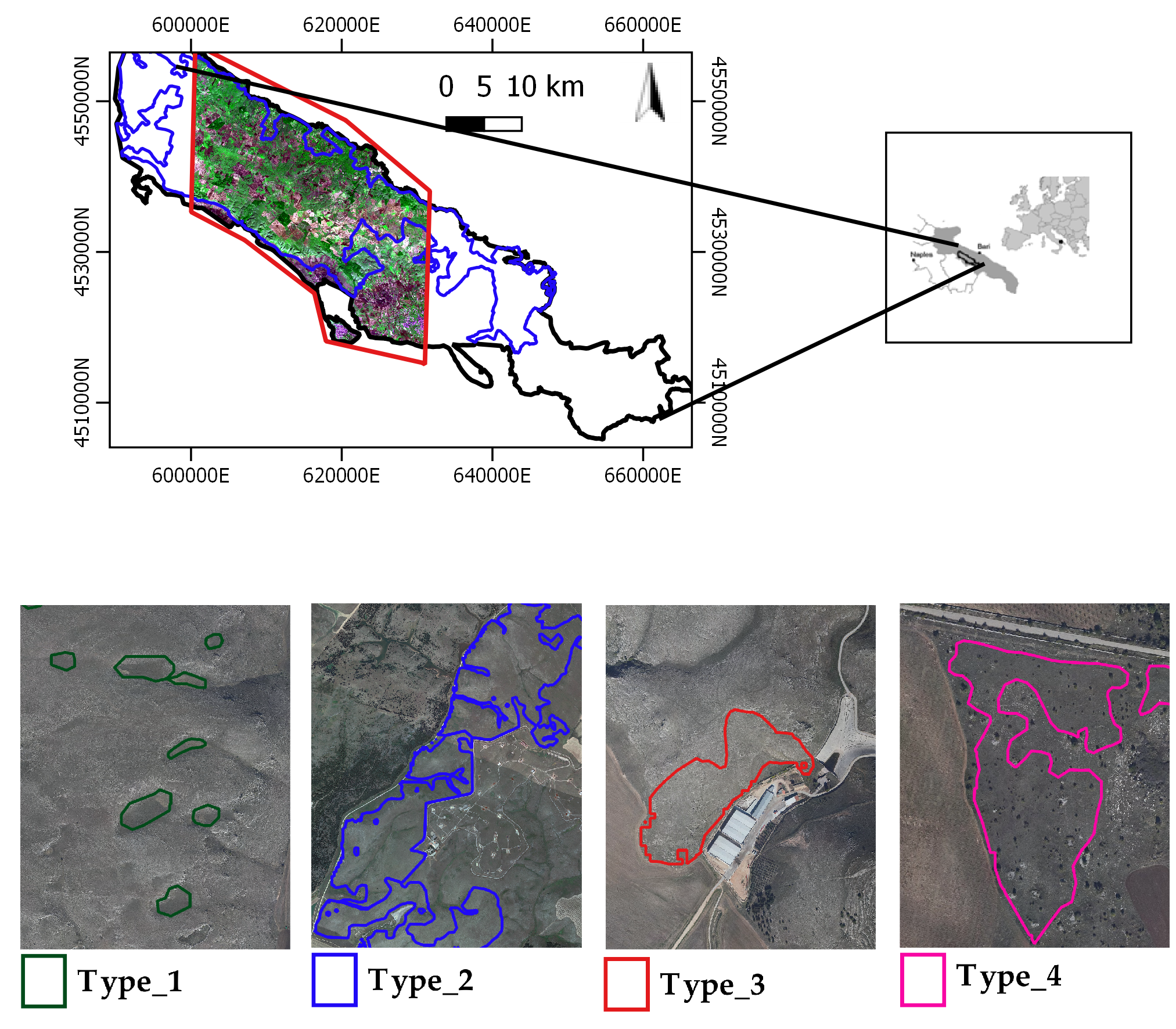
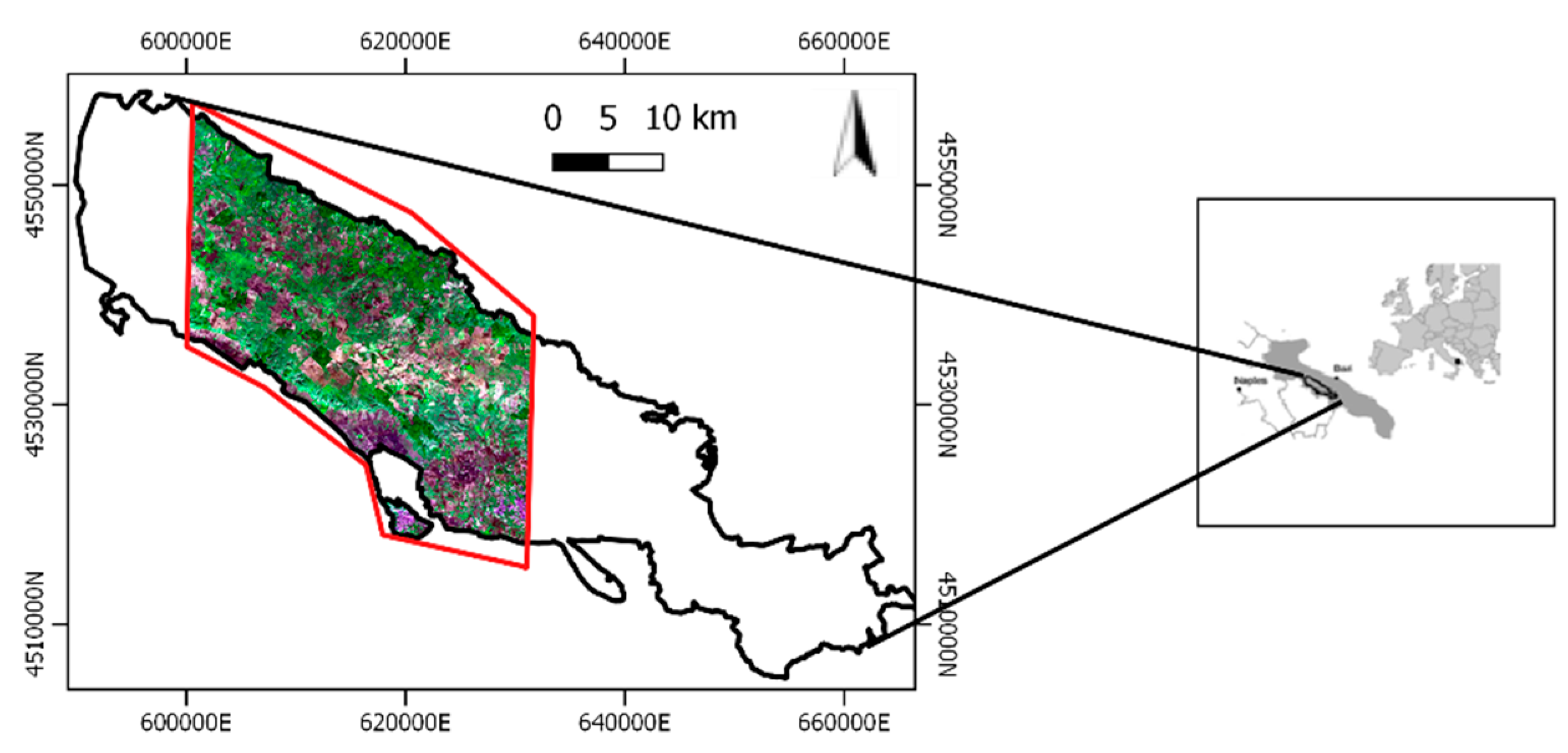
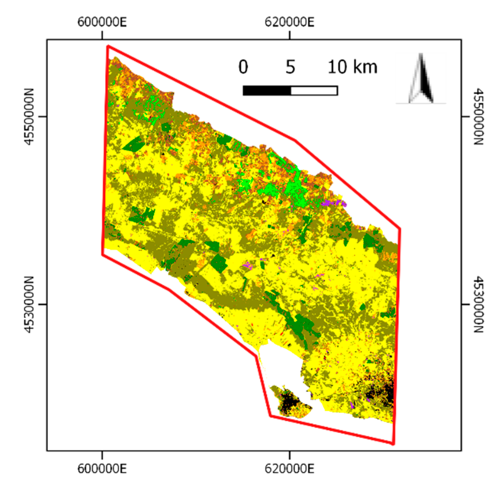
2.1. Study Area and Grassland Habitats Characterization
- the Common Agricultural Policy (CAP) which has driven the transformation of grassland pastures into agricultural (cereal crops intensification) areas by stone (rock) graining (clearance) that has induced soil erosion and sediment deposition in the aquifer system;
- the illegal waste and toxic mud dumping on transformed areas has caused heavy metal contamination of soils and aquifers;
- the below long-term average rainfall as a result of climate change;
2.2. Data Availability
2.2.1. Ground Truth Data
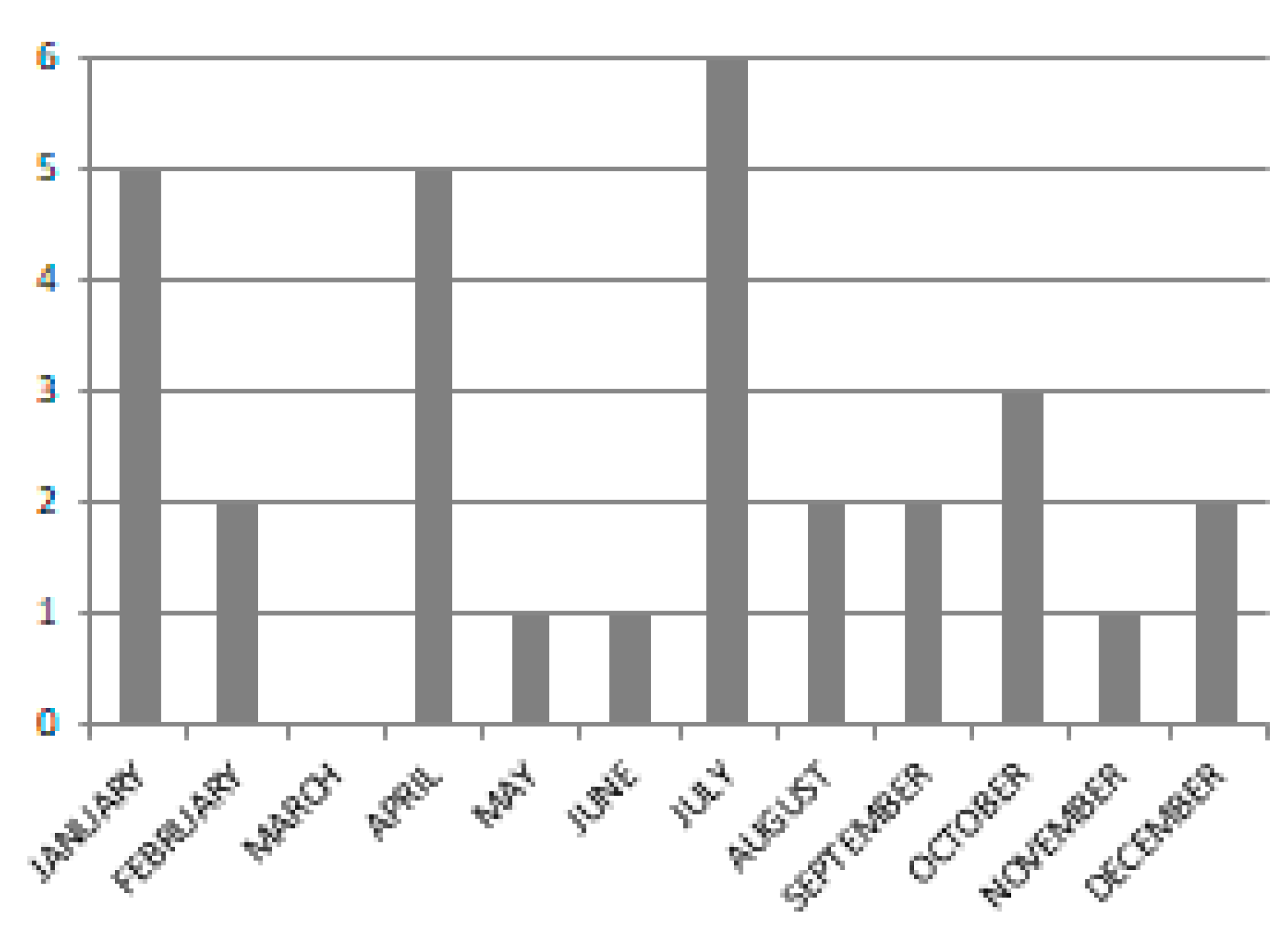
2.2.2. Satellite Data
2.2.3. Satellite Data Pre-Processing
- cropping according to the area of interest;
- spectral index extraction at the native spatial bands resolution;
- bilinear resampling to 10 m, when necessary. Indeed, 10 m was the final resolution adopted in our work. Different resampling approaches were tested. The bilinear one resulted the right compromise between minimization of artifacts and distortions introduced in the image as well as in the computational complexity.
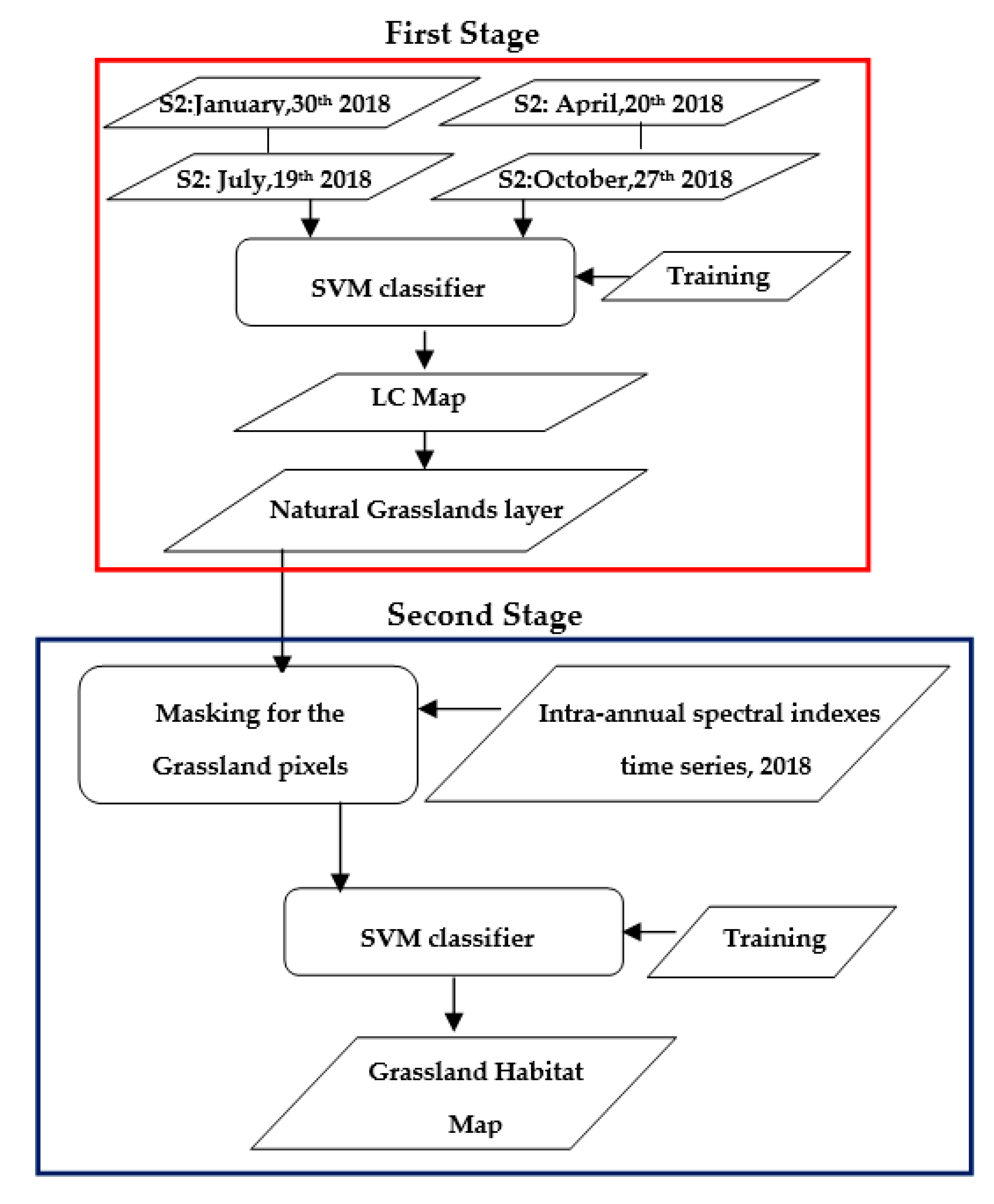
2.3. Two-Stage Algorithm for Habitat Mapping
2.3.1. First Stage
2.3.2. Second Stage
2.4. Accuracy Asssessment
3. Results
3.1. First Stage: Grassland Layer Extraction
3.2. Second Stage: Habitat Discrimination
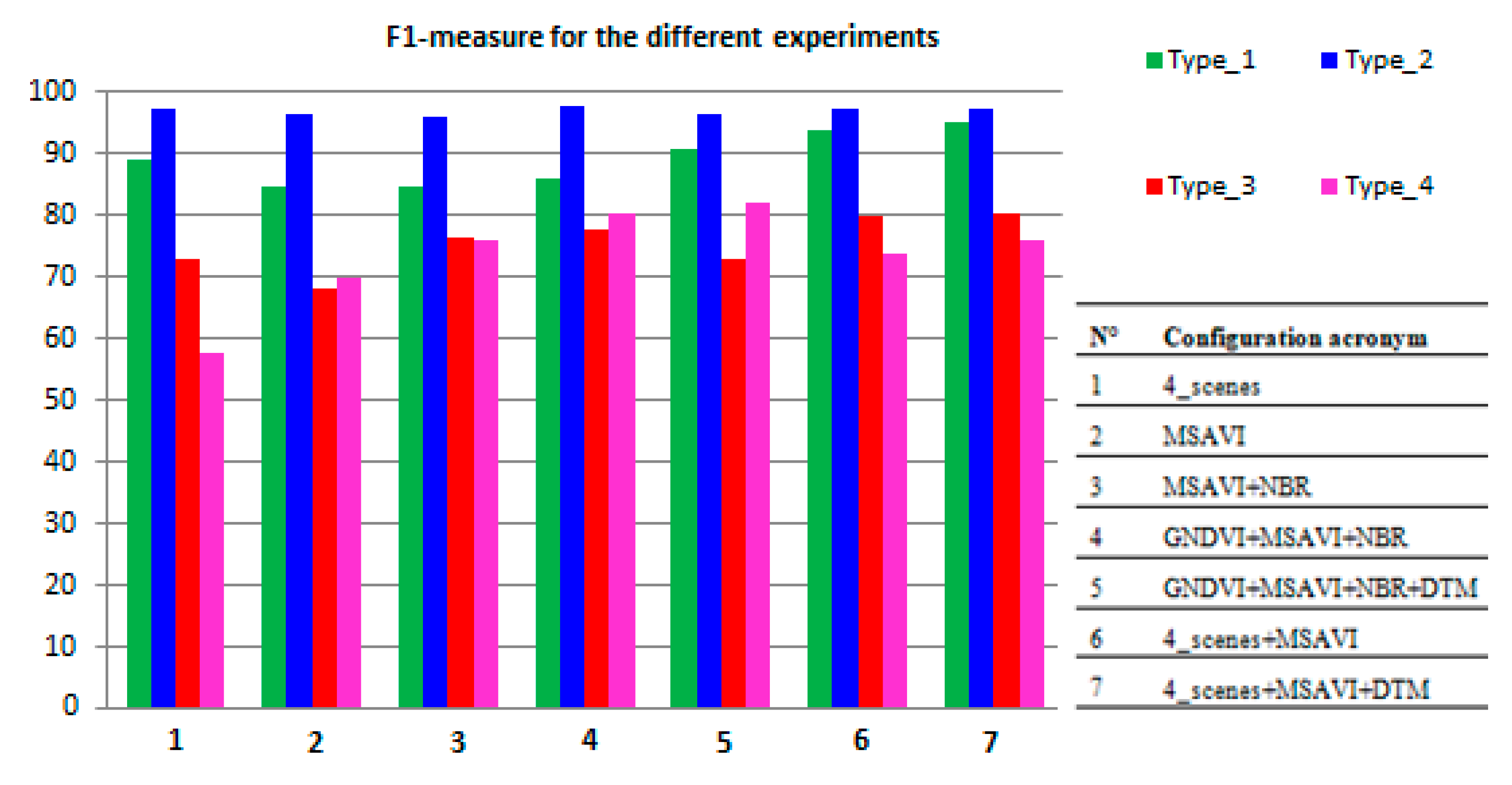
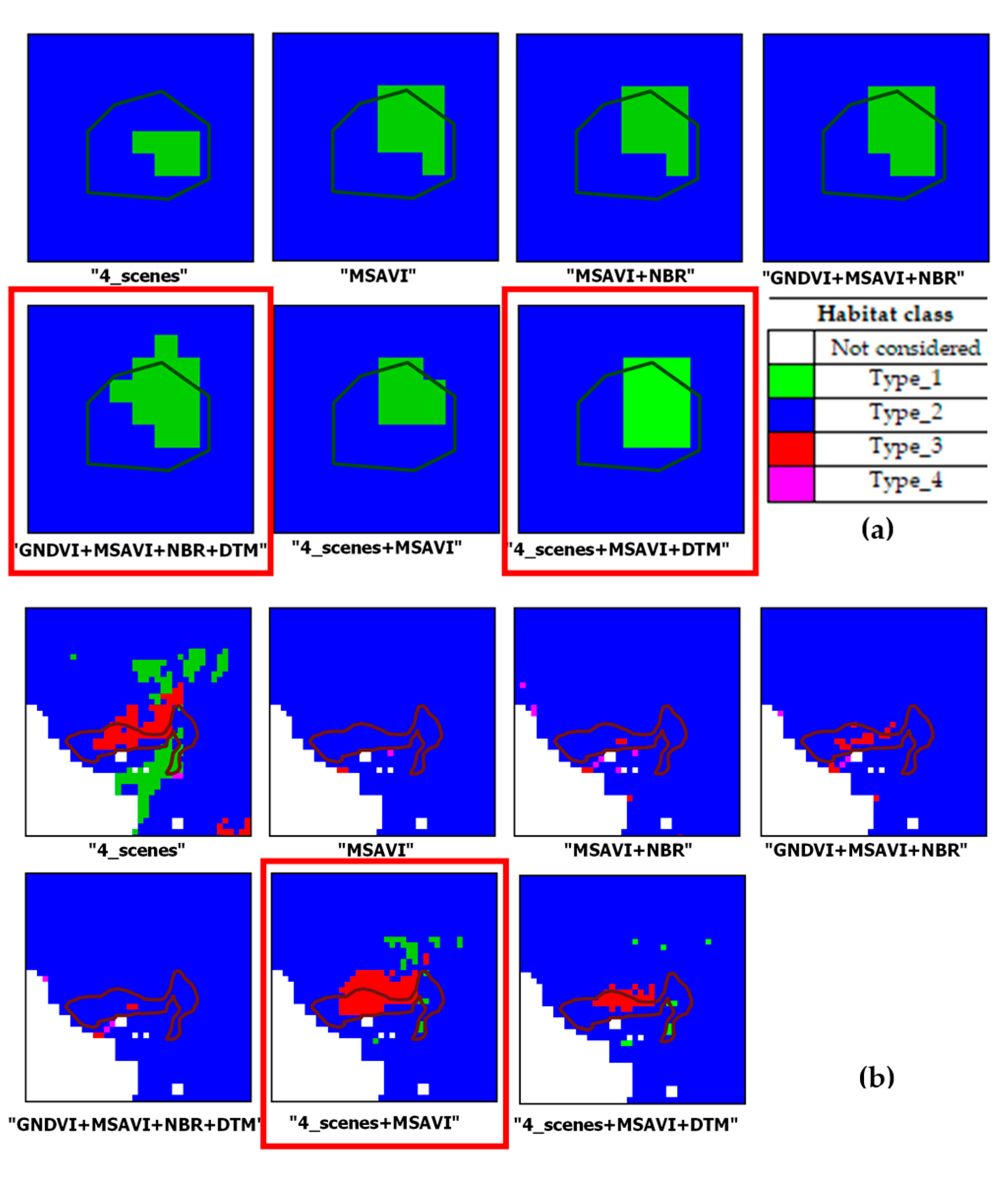
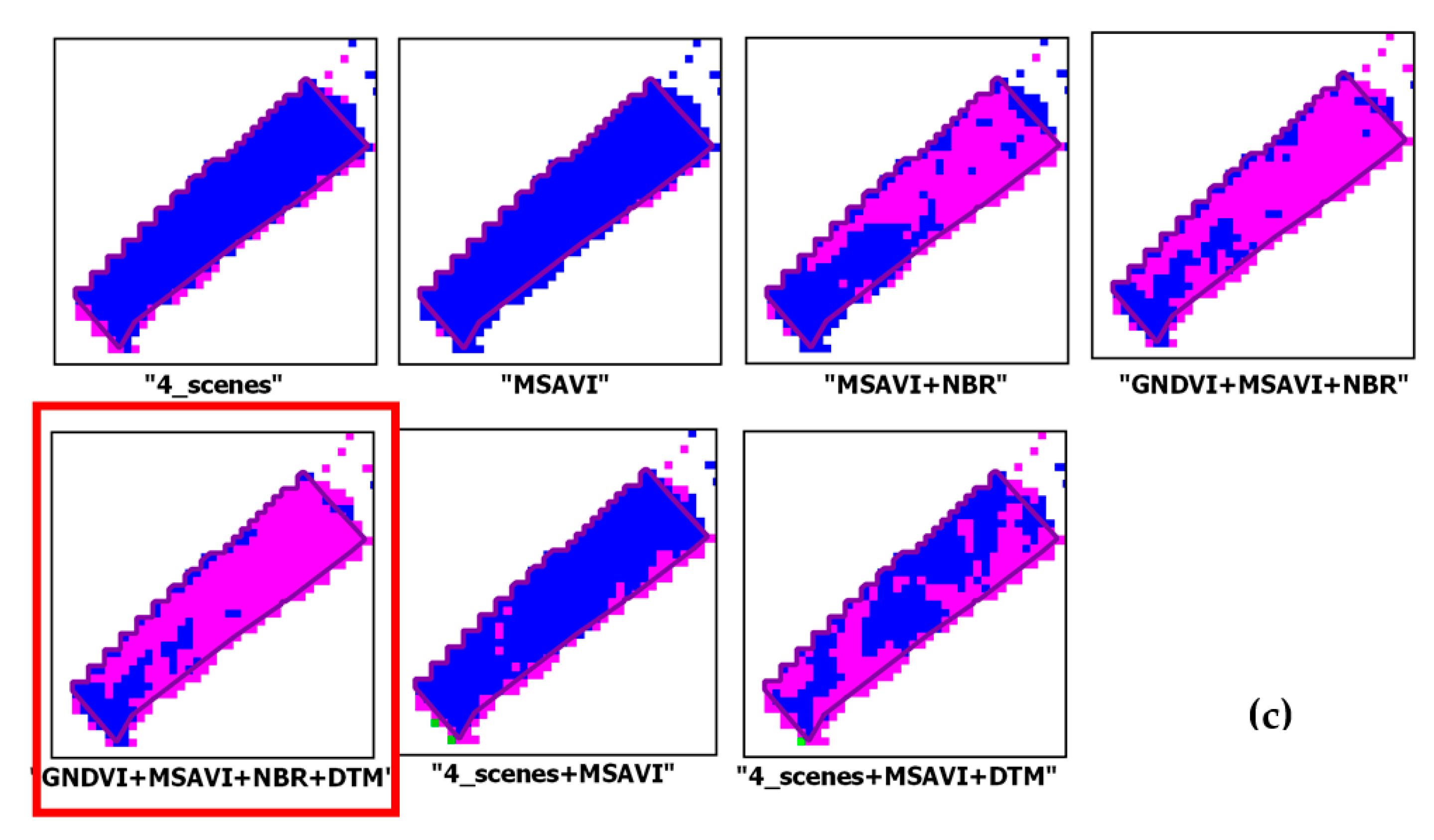
Combination of Different Configurations
4. Discussion
5. Conclusions
Author Contributions
Funding
Institutional Review Board Statement
Informed Consent Statement
Data Availability Statement
Acknowledgments
Conflicts of Interest
Appendix A

| Acquisition Date | Sensor |
|---|---|
| 2018-01-03 | S2A |
| 2018-01-05 | S2B |
| 2018-01-18 | S2B |
| 2018-01-25 | S2B |
| 2018-01-30° | S2A |
| 2018-02-12 | S2A |
| 2018-02-14 | S2B |
| No cloud free images in March | |
| 2018-04-08 | S2B |
| 2018-04-13 | S2A |
| 2018-04-20° | S2A |
| 2018-04-23 | S2A |
| 2018-04-30 | S2A |
| 2018-05-25 | S2B |
| 2018-06-12 | S2A |
| 2018-07-02 | S2A |
| 2018-07-09 | S2A |
| 2018-07-12 | S2A |
| 2018-07-14 | S2B |
| 2018-07-19° | S2A |
| 2018-07-22 | S2A |
| 2018-08-01 | S2A |
| 2018-08-28 | S2A |
| 2018-09-12 | S2B |
| 2018-09-22 | S2B |
| 2018-10-20 | S2A |
| 2018-10-25 | S2B |
| 2018-10-27° | S2A |
| 2018-11-09 | S2A |
| 2018-12-04 | S2B |
| 2018-12-09 | S2A |
References
- Schuster, C.; Schmidt, T.; Conrad, C.; Kleinschmit, B.; Forster, M. Grassland habitat mapping by intra-annual time-series analysis-Comparison of RapidEye and TerraSAR-X satellite data. Int. J. Appl. Earth Obs. GeoInf. 2015, 34, 25–34. [Google Scholar] [CrossRef]
- Hector, A.; Schmid, B.; Beierkuhnlein, C.; Caldeira, M.C.; Diemer, M.; Dimitrakopoulos, P.G.; Finn, J.A.; Freitas, H.; Giller, P.S.; Good, J.; et al. Plant diversity and productivity of European grasslands. Science 1999, 286, 1123–1127. [Google Scholar] [CrossRef] [PubMed] [Green Version]
- Fraser, L.H.; Pither, J.; Jentsch, A.; Sternberg, M.; Zobel, M.; Askarizadeh, D.; Bartha, S.; Beierkuhnlein, C.; Bennett, J.; Bittel, A.; et al. Worldwide evidence of a unimodal relationship between productivity and plant species richness. Science 2015, 349, 302–305. [Google Scholar] [CrossRef] [PubMed] [Green Version]
- Dengler, J.; Janišová, M.; Török, P.; Wellstein, C. Biodiversity of Palaearctic grasslands: A synthesis. Agric. Ecosyst. Environ. 2014, 182, 1–14. [Google Scholar] [CrossRef] [Green Version]
- O’Mara, F. The role of grasslands in food security and climate change. Ann. Bot. 2012, 110, 1263–1270. [Google Scholar] [CrossRef] [PubMed] [Green Version]
- Habel, J.C.; Dengler, J.; Janišová, M.; Török, P.; Wellstein, C.; Wiezik, M. European grassland ecosystems: Threatened hotspots of biodiversity. Biodivers. Conserv. 2013, 22, 2131–2138. [Google Scholar] [CrossRef] [Green Version]
- Newbold, T.; Hudson, L.N.; Arnell, A.P.; Contu, S.; De Palma, A.; Ferrier, S.; Hill, S.L.L.; Hoskins, A.J.; Lysenko, I.; Phillips, H.R.P.; et al. Has land use pushed terrestrial biodiversity beyond the planetary boundary? A global assessment. Science 2016, 353, 288–291. [Google Scholar] [CrossRef]
- Wellstein, C.; Poschlod, P.; Gohlke, A.; Chelli, S.; Campetella, G.; Rosbakh, S.; Canullo, R.; Kreyling, J.; Jentsch, A.; Beierkuhnlein, C. Effects of extreme drought on specific leaf area of grassland species: A meta-analysis of experimental studies in temperate and sub-Mediterranean systems. Glob. Chang. Biol. 2017, 23, 2473–2481. [Google Scholar] [CrossRef]
- Council Directive 92/43/EEC. Available online: https://eur-lex.europa.eu/legal-content/EN/TXT/?uri=celex%3A31992L0043 (accessed on 1 July 2013).
- Council Directive 2009/147/EEC. Available online: https://eur-lex.europa.eu/legal-content/EN/TXT/?uri=CELEX%3A32009L0147 (accessed on 26 June 2019).
- CBD. Available online: https://www.cbd.int/convention/articles/?a=cbd-01 (accessed on 11 February 2006).
- Natura 2000, EU. Available online: https://ec.europa.eu/environment/nature/natura2000/index_en.htm (accessed on 11 November 2008).
- Buck, O.; Garcia Millàn, V.E.; Klink, A.; Pakzad, K. Using information layers for mapping grassland habitat distribution at local to regional scales. Int. J. Appl. Earth Obs. Geoinf. 2015, 37, 83–89. [Google Scholar] [CrossRef]
- Mehner, H.; Cutler, M.; Fairbairn, D.; Thompson, G. Remote sensing of upland vegetation: The potential of high spatial resolution satellite sensors. Glob. Ecol. Biogeogr. 2004, 13, 359–369. [Google Scholar] [CrossRef]
- Hill, M.J.; Ticehurst, C.J.; Lee, J.; Fellow, L.; Grunes, M.R.; Donald, G.E.; Henry, D. Integration of optical and radar classifications for mapping pasture type in Western Australia. IEEE Trans. Geosci. Remote Sens. 2005, 43, 1665–1681. [Google Scholar] [CrossRef]
- Schmidtlein, S.; Zimmermann, P.; Schüpferling, R.; Weiß, C. Mapping the floristic continuum: Ordination space position estimated from imaging spectroscopy. J. Veg. Sci. 2007, 18, 131–140. [Google Scholar] [CrossRef]
- Schuster, C.; Ali, I.; Lohmann, P.; Frick, A.; Förster, M.; Kleinschmit, B. Towards detecting swath events in TerraSAR-X time-series to establish Natura 2000 grassland habitat swath management as monitoring parameter. Remote Sens. 2011, 3, 1308–1322. [Google Scholar] [CrossRef] [Green Version]
- Wright, C.K.; Wimberly, M.C. Recent land use change in the Western Corn Belt threatens grasslands and wetlands. Proc. Natl. Acad. Sci. USA 2013. [Google Scholar] [CrossRef] [PubMed] [Green Version]
- Feilhauer, H.; Thonfeld, F.; Faude, U.; He, K.S.; Rocchini, D.; Schmidtlein, S. Assessing floristic composition with multispectral sensors—A comparison based on monotemporal and multiseasonal field spectra. Int. J. Appl. Earth Observ. Geoinf. 2013, 21, 218–229. [Google Scholar] [CrossRef]
- Nagendra, H.; Lucas, R.M.; Honrado, J.P.; Jongman, R.; Tarantino, C.; Adamo, P.; Mairota, P. Remote sensing for conservation monitoring: Assessing protected areas, habitat extent, habitat condition, species diversity and threats. Ecol. Indic. 2013, 33, 45–59. [Google Scholar] [CrossRef]
- Turner, W.; Spector, S.; Gardiner, N.; Fladeland, M.; Sterling, E.; Steininger, M. Remote sensing for biodiversity science and conservation. Trends Ecol. Evol. 2003, 18, 306–314. [Google Scholar] [CrossRef]
- Strand, H.; Höft, R.; Strittholt, J.; Horning, N.; Miles, L.; Fosnight, E.; Turner, W. Sourcebook on Remote Sensing and Biodiversity Indicators; Technical Series; Secretariat of the Convention on Biological Diversity: Montreal, QC, Canada, 2007. [Google Scholar]
- Wang, K.; Franklin, S.E.; Guo, X.; Cattet, M. Remote sensing of ecology, bio-diversity and conservation: A review from the perspective of remote sensing specialists. Sensors 2010, 10, 9647–9667. [Google Scholar] [CrossRef]
- Franke, J.; Keuck, V.; Siegert, F. Assessment of grassland use intensity by remote sensing to support conservation schemes. J. Nat. Conserv. 2012, 20, 125–134. [Google Scholar] [CrossRef]
- Corbane, C.; Alleaume, S.; Deshayes, M. Mapping natural habitats using remote sensing and sparse partial least square discriminant analysis. Int. J. Remote Sens. 2013, 34, 7625–7647. [Google Scholar] [CrossRef] [Green Version]
- Zlinszky, A.; Schroiff, A.; Kania, A.; Deák, B.; Mücke, W.; Vári, A.; Székely, B.; Pfeifer, N. Categorizing Grassland Vegetation with Full-Waveform Airborne Laser Scanning: A Feasibility Study for Detecting Natura 2000 Habitat Types. Remote Sens. 2014, 6, 8056–8087. [Google Scholar] [CrossRef] [Green Version]
- Landmann, T.; Piiroinen, R.; Makori, D.M.; Abdel-Rahman, E.M.; Makau, S.; Pellikka, P.; Raina, S.K. Application of hyperspectral remote sensing for flower mapping in African savannas. Remote Sens. Environ. 2015, 166, 50–60. [Google Scholar] [CrossRef]
- Möckel, T.; Dalmayne, J.; Schmid, B.C.; Prentice, H.C.; Hall, K. Airborne hyperspectral data predict fine-scale plant species diversity in grazed dry grasslands. Remote Sens. 2016, 8, 133. [Google Scholar] [CrossRef] [Green Version]
- Gholizadeh, H.; Gamon, J.A.; Townsend, P.A.; Zygielbaum, A.I.; Helzer, C.J.; Hmimina, G.Y.; Yu, R.; Moore, R.M.; Schweiger, A.K.; Cavender-Bares, J. Detecting prairie biodiversity with airborne remote sensing. Remote Sens. Environ. 2019, 221, 38–49. [Google Scholar] [CrossRef]
- Oldeland, J.; Wesuls, D.; Rocchini, D.; Schmidt, M.; Jürgens, N. Does using species abundance data improve estimates of species diversity from remotely sensed spectral heterogeneity? Ecol. Indic. 2010, 10, 390–396. [Google Scholar] [CrossRef]
- Marcinkowska-Ochtyra, A.; Gryguc, K.; Ochtyra, A.; Kopeć, D.; Jarocinska, A.; Sławik, L. Multitemporal Hyperspectral Data Fusion with Topographic Indices—Improving Classification of Natura 2000 Grassland Habitats. Remote Sens. 2019, 11, 2264. [Google Scholar] [CrossRef] [Green Version]
- Wen, Q.; Zhang, Z.; Liu, S.; Wang, X.; Wang, C. Classification of grassland types by MODIS time-series images in Tibet, China. IEEE J. Sel. Top. Appl. Earth Obs. Rem. Sens. 2010, 3, 3. [Google Scholar] [CrossRef]
- Copernicus ESA Program. Available online: https://www.esa.int/Applications/Observing_the_Earth/Copernicus (accessed on 22 June 2018).
- Drusch, M.; Bello, U.D.; Carlier, S.; Colin, O.; Fernandez, V.; Gascon, F.; Hoersch, B.; Isola, C.; Laberinti, P.; Martimort, P.; et al. Sentinel-2: ESA’s optical high-resolution mission for GMES operational services. Remote Sens. Environ. 2012, 120, 25–36. [Google Scholar] [CrossRef]
- Fauvel, M.; Lopes, M.; Dubo, T.; Rivers-Moore, J.; Frison, P.; Gross, N.; Ouin, A. Prediction of plant diversity in grasslands using Sentinel-1 and -2 satellite image time-series. Remote Sens. Environ. 2020, 237, 111536. [Google Scholar] [CrossRef]
- Rapinel, S.; Mony, C.; Lecoq, L.; Clément, B.; Thomas, A.; Hubert-Moy, L. Evaluation of Sentinel-2 time-series for mapping floodplain grassland plant communities. Remote Sens. Environ. 2019, 223, 115–129. [Google Scholar] [CrossRef]
- Groβe-Stoltenbeg, A.; Hellmann, C.; Werner, C.; Oldeland, J.; Thiele, J. Evaluation of continuous VNIR-SWIR pectra versus narrowband hyperspectral indices to discriminate the invasive Acacia longifolia within a Mediterranean dune ecosystem. Remote Sens. 2016, 8, 334. [Google Scholar] [CrossRef] [Green Version]
- Vapnik, V.N. The Nature of Statistical Learning Theory; Springer: New York, NY, USA, 1995. [Google Scholar]
- Vapnik, V.N. Statistical Learning Theory; Wiley: New York, NY, USA, 1998. [Google Scholar]
- Rabe, A.; van der Linden, S.; Hostert, P. Simplifying Support Vector Machines for classification of hyperspectral imagery and selection of relevant features. In Proceedings of the 2nd Workshop of Hyperspectral Image and Signal Processing: Evolution in Remote Sensing (WHISPERS), Reykjavik, Iceland, 14–16 June 2010. [Google Scholar] [CrossRef]
- Grabska, E.; Frantz, D.; Ostapowicz, K. Evaluation of machine learning algorithms for forest stand species mapping using Sentinel-2 imagery and environmental data in the Polish Carpathians. Remote Sens. Environ. 2020, 251, 112103. [Google Scholar] [CrossRef]
- Maxwell, A.E.; Warner, T.A.; Fang, F. Implementation of machine-learning classification in remote sensing: An applied review. Int. J. Remote Sens. 2018, 39, 2784–2817. [Google Scholar] [CrossRef] [Green Version]
- Forte, L.; Perrino, E.V.; Terzi, M. Le praterie a Stipa austroitalica Martinovsky ssp. austroitalica dell’Alta Murgia (Puglia) e della Murgia Materana (Basilicata). Fitosociologia 2005, 42, 83–103. [Google Scholar]
- Mairota, P.; Leronni, V.; Xi, W.; Mladenoff, D.; Nagendra, H. Using spatial simulations of habitat modification for adaptive management of protected areas: Mediterranean grassland modification by woody plant encroachment. Environ. Conserv. 2013, 41, 144–146. [Google Scholar] [CrossRef]
- Mairota, P.; Cafarelli, B.; Labadessa, R.; Lovergine, F.; Tarantino, C.; Lucas, R.M.; Nagendra, H.; Didham, R.K. Very high resolution Earth observation features for monitoring plant and animal community structure across multiple spatial scales in protected areas. Int. J. Appl. Earth Obs. Geoinf. 2015, 37, 100–105. [Google Scholar] [CrossRef]
- Sutter, G.C.; Brigham, R.M. Avifaunal and habitat changes resulting from conversion of native prairie tocrested wheat grass: Patterns at songbird community and species levels. Can. J. Zool. 1998, 76, 869–875. [Google Scholar] [CrossRef]
- Brotons, L.; Pons, P.; Herrando, S. Colonization of dynamic Mediterranean landscapes: Where do birds come from after fire? J. Biogeogr. 2005, 32, 789–798. [Google Scholar] [CrossRef]
- Tarantino, C.; Casella, F.; Adamo, M.; Lucas, R.; Beierkuhnlein, C.; Blonda, P. Ailanthus altissima mapping from multi-temporal very high resolution satellite images. ISPRS J. Photogram. Remote Sens. 2019, 147, 90–103. [Google Scholar] [CrossRef]
- Davies, C.E.; Moss, D. EUNIS Habitat Classification. In Final Report to the European Topic Centre of Nature Protection and Biodiversity; European Environment Agency: Swindon, UK, 2002. [Google Scholar]
- Bartolucci, F.; Peruzzi, L.; Galasso, G.; Albano, A.; Alessandrini, A.; Ardenghi, N.M.G.; Astuti, G.; Bacchetta, G.; Ballelli, S.; Banfi, E.; et al. An updated checklist of the vascular flora native to Italy. Plant Biosyst. 2018, 152, 179–303. [Google Scholar] [CrossRef]
- Biondi, E.; Blasi, C. Prodromo della Vegetazione Italiana 2015. Ministero dell’Ambiente e della Tutela del Territorio e del Mare. Available online: http://www.prodromo-vegetazione-italia.org/ (accessed on 1 March 2015).
- Perrino, E.V.; Brunetti, G.; Farrag, K. Plant Communities in Multi-Metal Contaminated Soils: A Case Study in the National Park of Alta Murgia (Apulia Region—Southern Italy). Int. J. Phytoremediat. 2014, 16, 871–888. [Google Scholar] [CrossRef]
- Congalton, R.G.; Gu, J.; Yadav, K.; Thenkabail, P.; Ozdogan, M. Global Land Cover Mapping: A Review and Uncertainty Analysis. Remote Sens. 2014, 6, 12070–12093. [Google Scholar] [CrossRef] [Green Version]
- Di Gregorio, A.; Jansen, L.J.M. Land Cover Classification System (LCCS): Classification Concepts and User Manual; Food and Agriculture Organization of the United Nations: Rome, Italy, 2005. [Google Scholar]
- Lucas, R.; Tomaselli, V.; Mitchell, A. Deliverable 4.2 (EO Biophysical Parameters, Land Use and Habitats Extraction Modules) of the Horizon2020 Project “ECOPOTENTIAL: Improving Future Ecosystem Benefits through Earth Observations” (G.A. 641762). Available online: http://www.ECOPOTENTIAL-project.eu (accessed on 5 March 2020).
- Masò, J.; Domingo-Marimon, C.; Lucas, R. Deliverable 10.3 of the Horizon2020 Project “ECOPOTENTIAL: Improving Future Ecosystem Benefits through Earth Observations” (G.A. 641762). Implementation of Apps. Research Report. 2018. Available online: http://www.ECOPOTENTIAL-project.eu (accessed on 5 March 2020).
- Tomaselli, V.; Dimopoulos, P.; Marangi, C.; Kallimanis, A.S.; Adamo, M.; Tarantino, C.; Panitsa, M.; Terzi, M.; Veronico, G.; Lovergine, F.; et al. Translating land cover/land use classifications to habitat taxonomies for landscape monitoring: A Mediterranean assessment. Landsc. Ecol. 2013, 28, 905–930. [Google Scholar] [CrossRef] [Green Version]
- Adamo, M.; Tarantino, C.; Tomaselli, V.; Kosmidou, V.; Petrou, Z.; Manakos, I.; Lucas, R.M.; Mücher, C.A.; Veronico, G.; Marangi, C.; et al. Expert knowledge for translating land cover/use maps to general habitat categories (GHC). Landsc. Ecol. 2014, 29, 1045–1067. [Google Scholar] [CrossRef] [Green Version]
- Lucas, R.M.; Blonda, P.; Bunting, P.F.; Jones, G.; Inglada, J.; Arias, M.; Kosmidou, V.; Petrou, Z.; Manakos, I.; Adamo, M.; et al. The Earth observation data for habitat monitoring (EODHaM) system. Int. J. Appl. Earth Obs. Geoinf. 2015, 37, 17–28. [Google Scholar] [CrossRef]
- Adamo, M.; Tarantino, C.; Tomaselli, V.; Veronico, G.; Nagendra, H.; Blonda, P. Habitat mapping of coastal wetlands using expert knowledge and Earth observation data. J. Appl. Ecol. 2016, 53, 1521–1532. [Google Scholar] [CrossRef]
- Gavish, Y.; O’Connel, J.; Marsh, C.J.; Tarantino, C.; Blonda, P.; Tomaselli, V.; Kunin, W.E. Comparing the performance of flat and hierarchical Habitat/Land-Cover classification models in a NATURA 2000 site. ISPRS J. Photogram. Remote Sens. 2018, 136, 1–12. [Google Scholar] [CrossRef]
- Adamo, M.; Tomaselli, V.; Tarantino, C.; Vicario, S.; Veronico, G.; Lucas, R.; Blonda, P. Knowledge-based classification of grassland ecosystem based on multi-temporal WorldView-2 data and FAO-LCCS taxonomy. Remote Sens. 2020, 12, 1447. [Google Scholar] [CrossRef]
- Braun-Blanquet, J. Pflanzensoziologie: Grundzüge der Vegetationskunde; Plant Sociology Basics of Vegetation Science; Springer: Berlin/Heidelberg, Germany, 1964; pp. 287–399. [Google Scholar]
- Westhoff, V.; van der Maarel, E. The Braun-Blanquet Approach. In Classification of Plant Communities; Whittaker, R.H., Ed.; Junk: The Hague, The Netherlands, 1978; pp. 287–399. [Google Scholar]
- EU. Habitats Manual, Interpretation Manual of European Union habitats: 1–144. 2013. Available online: http://ec.europa.eu/environment/nature/legislation/habitatsdirective/docs/Int_Manual_EU28.pdf (accessed on 1 April 2013).
- Biondi, E.; Blasi, C.; Burrascano, S.; Casavecchia, S.; Copiz, R.; Del Vico, E.; Galdenzi, D.; Gigante, D.; Lasen, C.; Spampinato, G.; et al. Manuale Italiano di Interpretazione Degli Habitat della Direttiva 92/43/CEE. MATTM-DPN, SBI. 2010. Available online: http://vnr.unipg.it/habitat/index.jsp (accessed on 1 December 2007).
- Van der Maarel, E. Transformation of cover-abundance values in phytosociology and its effects on community similarity. Vegetation 1979, 39, 97–114. [Google Scholar]
- Sokal, R.R.; Michener, C.D. A Statistical Method for Evaluating Systematic Relationships. Univ. Kansas Sci. Bull. 1958, 38, 1409–1438. [Google Scholar]
- Biondi, E.; Burrascano, S.; Casavecchia, S.; Copiz, R.; Del Vico, E.; Galdenzi, D.; Gigante, D.; Lasen, C.; Spampinato, G.; Venanzoni, R.; et al. Diagnosis and syntaxonomic interpretation of Annex I Habitats (Dir. 92/43/ EEC) in Italy at the alliance level. Plant Sociol. 2012, 49, 5–37. [Google Scholar]
- USGS Portal. Available online: https://earthexplorer.usgs.gov/ (accessed on 9 May 2018).
- ESA Technical Guide. Available online: https://sentinel.esa.int/web/sentinel/technical-guides/sentinel-2-msi/level-2a-processing (accessed on 26 March 2018).
- Puglia Region Portal. Available online: www.sit.puglia.it (accessed on 1 February 2014).
- Gitelson, A.; Kaufman, Y.; Merzlyak, M.N. Use of green channel in remote sensing of global vegetation from EOS-MODIS. Remote Sens. Environ. 1996, 58, 289–298. [Google Scholar] [CrossRef]
- Barati, S.; Rayegani, B.; Saati, M.; Sharifi, A.; Nasri, M. Comparison the accuracies of different spectral indices for estimation of vegetation cover fraction in sparse vegetated areas. Egypt. J. Remote Sens. Space Sci. 2011, 14, 49–56. [Google Scholar] [CrossRef] [Green Version]
- Qi, J.; Chehbouni, A.; Huete, A.R.; Kerr, Y.H. Modified Soil Adjusted Vegetation Index (MSAVI). Remote Sens. Environ. 1994, 48, 119–126. [Google Scholar] [CrossRef]
- Lopez-Garcia, M.; Caselles, V. Mapping burns and natural reforestation using Thematic Mapper data. Geocarto Int. 1991, 6, 31–37. [Google Scholar] [CrossRef]
- Lutes, D.C.; Keane, R.E.; Caratti, J.F.; Key, C.H.; Benson, N.C.; Sutherland, S.; Gangi, L.J. General Technical Report RMRS-GTR-164-CD; FIREMON: Fire Effects Monitoring and Inventory System, Ed.; Department of Agriculture, Forest Service, Rocky Mountains Research Station: Fort Collins, CO, USA, 2006. [CrossRef]
- Vicario, S.; Adamo, M.; Alcaraz-Segura, D.; Tarantino, C. Bayesian Harmonic Modelling of Sparse and Irregular Satellite Remote Sensing Time-series of Vegetation Indexes: A Story of Clouds and Fires. Remote Sens. 2020, 12, 83. [Google Scholar] [CrossRef] [Green Version]
- Asner, G.P.; David, B. Lobell. A Biogeophysical Approach for Automated SWIR Unmixing of Soils and Vegetation. Remote Sens. Environ. 2000, 74.1, 99–112. [Google Scholar] [CrossRef]
- Zhang, K.; Ge, X.; Shen, P.; Li, W.; Liu, X.; Cao, Q.; Zhu, Y.; Cao, W.; Tian, Y. Predicting Rice Grain Yield Based on Dynamic Changes in Vegetation Indexes during Early to Mid-Growth Stages. Remote Sens. 2019, 11, 387. [Google Scholar] [CrossRef] [Green Version]
- Main, R.; Cho, M.A.; Mathieu, R.; O’Kennedy, M.M.; Ramoelo, A.; Koch, S. An investigation into robust spectral indices for leaf chlorophyll estimation. ISPRS J. Photogramm. Remote Sens. 2011, 66, 751–761. [Google Scholar] [CrossRef]
- Harris Geospatial Solutions. Available online: www.harris.com/solution/envi (accessed on 5 March 2015).
- Huang, C.; Davis, L.S.; Townshend, J.R.G. An assessment of support vector machines for land cover classification. Int. J. Remote Sens. 2002, 23, 725–749. [Google Scholar] [CrossRef]
- Mountrakis, G.; Im, J.; Ogole, C. Support vector machines in remote sensing: A review. ISPRS J. Photogramm. Remote Sens. 2011, 66, 247–259. [Google Scholar] [CrossRef]
- Foody, G.M.; Mathur, A. A relative evaluation of multiclass image classification by support vector machines. IEEE Trans. Geosci. Remote Sens. 2004, 6, 1335–1343. [Google Scholar] [CrossRef] [Green Version]
- Waske, B.; Van der Linden, S. Classifying multilevel imagery from SAR and optical sensors by decision fusion. IEEE Trans. Geosci. Remote Sens. 2008, 46, 1457–1466. [Google Scholar] [CrossRef]
- Othman, A.A.; Al-Maamar, A.F.; Al-Manmi, D.A.; Liesenberg, V.; Hasan, S.E.; Obaid, A.K.; Al-Quraishi, A.M. GIS-based modeling for selection of Dam sites in the Kurdistan region, Iraq. Int. J. Geo-Inf. 2020, 9, 244. [Google Scholar] [CrossRef] [Green Version]
- Othman, A.A.; Gloaguen, R. Improving lithological mapping by SVM classification of spectral and morphological features: The discovery of a new chromite body in the Mawat ophiolite complex (Kurdistan, NE Iraq). Remote Sens. 2014, 6, 6867–6896. [Google Scholar] [CrossRef] [Green Version]
- Yang, X. Parameterizing support vector machines for land cover classification. Photogramm. Eng. Remote Sens. 2011, 77, 27–38. [Google Scholar] [CrossRef]
- Othman, A.; Al-Saady, Y.; Al-Khafaji, A.; Gloaguen, R. Environmental change detection in the central part of Iraq using remote sensing data and GIS. Arab. J. Geosci. 2014, 7, 1017–1028. [Google Scholar] [CrossRef]
- Olofsson, P.; Foody, G.M.; Stehman, S.V.; Woodcock, C.E. Making better use of accuracy data in land change studies: Estimating accuracy and area and quantifying uncertainty using stratified estimation. Remote Sens. Environ. 2013, 129, 122–131. [Google Scholar] [CrossRef]
- Olofsson, P.; Foody, G.M.; Herold, M.; Stehman, S.V.; Woodcock, C.E.; Wulder, M.A. Good practices for estimating area and assessing accuracy of land change. Remote Sens. Environ. 2014, 148, 42–57. [Google Scholar] [CrossRef]
- Tarantino, C.; Adamo, M.; Lucas, R.; Blonda, P. Detection of changes in semi-natural grasslands by cross correlation analysis with WorldView-2 images and new Landsat 8 data. Remote Sens. Environ. 2016, 175, 65–72. [Google Scholar] [CrossRef]
- Congalton, R.G.; Kass, G. Assessing the Accuracy of Remotely Sensed Data: Principle and Practices, 2nd ed.; Taylor & Francis Group: Abingdon, UK, 2009; ISBN 9781420055122. [Google Scholar]
- Sasaki, Y. The Truth of the F-Measure; 2007. Available online: https://www.toyota-ti.ac.jp/Lab/Denshi/COIN/people/yutaka.sasaki/F-measure-YS-26Oct07.pdf (accessed on 26 October 2007).
- Halder, A.; Ghosh, A.; Ghosh, S. Aggregation pheromone density based pattern classification. Fundam. Inform. 2009, 92, 345–362. [Google Scholar]
- Schuster, C.; Förster, M.; Kleinschmit, B. Testing the red edge channel for improving land-use classifications based on high-resolution multi-spectral satellite data. Int. J. Remote Sens. 2012, 33, 5583–5599. [Google Scholar] [CrossRef]
- Baumann, M.; Ozdogan, M.; Kuemmerle, T.; Wendland, K.J.; Esipova, E.; Radeloff, V.C. Using the Landsat record to detect forest-cover changes during and after the collapse of the Soviet Union in the temperate zone of European Russia. Remote Sens. Environ. 2012, 124, 174–184. [Google Scholar] [CrossRef]
- Tulyakov, S.; Jaeger, S.; Govindaraju, V.; Doermann, D. Review of classifier combination methods. Mach. Learn. Doc. Anal. Recognit. 2008, 90, 361–386. [Google Scholar]
- Xiaoshuang, M.; Huanfeng, S.; Jie, Y.; Liangpei, Z.; Pingxiang, L. Polarimetric-Spatial Classification of SAR Images Based on the Fusion of Multiple Classifiers. IEEE J. Sel. Top. Appl. Earth Obs. Remote Sens. 2014, 7, 961–971. [Google Scholar] [CrossRef]
- Xue, Y. An overview of Overfitting and its solutions. J. Phys. Conf. Ser. 2019. [Google Scholar] [CrossRef]
- Clerici, N.; Weissteiner, C.J.; Halabuk, A.; Hazeu, G.; Roerink, G.; Mücher, S. Phenology Related Measures and Indicators at Varying Spatial Scales; Alterra Report; 2012; p. 2259. ISSN 1566-7197. Available online: https://edepot.wur.nl/199907 (accessed on 1 January 2012).
- Jönsson, P.; Cai, Z.; Melaas, E.; Friedl, M.A.; Eklundh, L. A Method for Robust Estimation of Vegetation Seasonality from Landsat and Sentinel-2 Time Series Data. Remote Sens. 2018, 10, 635. [Google Scholar] [CrossRef] [Green Version]
- Griffiths, P.; Nendel, C.; Hostert, P. Intra-annual reflectance composites from Sentinel-2 and Landsat for national-scale crop and land cover mapping. Remote Sens. Environ. 2019, 220, 135–151. [Google Scholar] [CrossRef]
- Foody, G.M.; Boyd, D.S.; Sanchez-Hernandez, C. Mapping a specific class with an ensemble of classifiers. Int. J. Remote Sens. 2007, 28, 1733–1746. [Google Scholar] [CrossRef]


| Types | Description | Code in Annex I to the Habitat Directive and (/) Eunis Taxonomies |
|---|---|---|
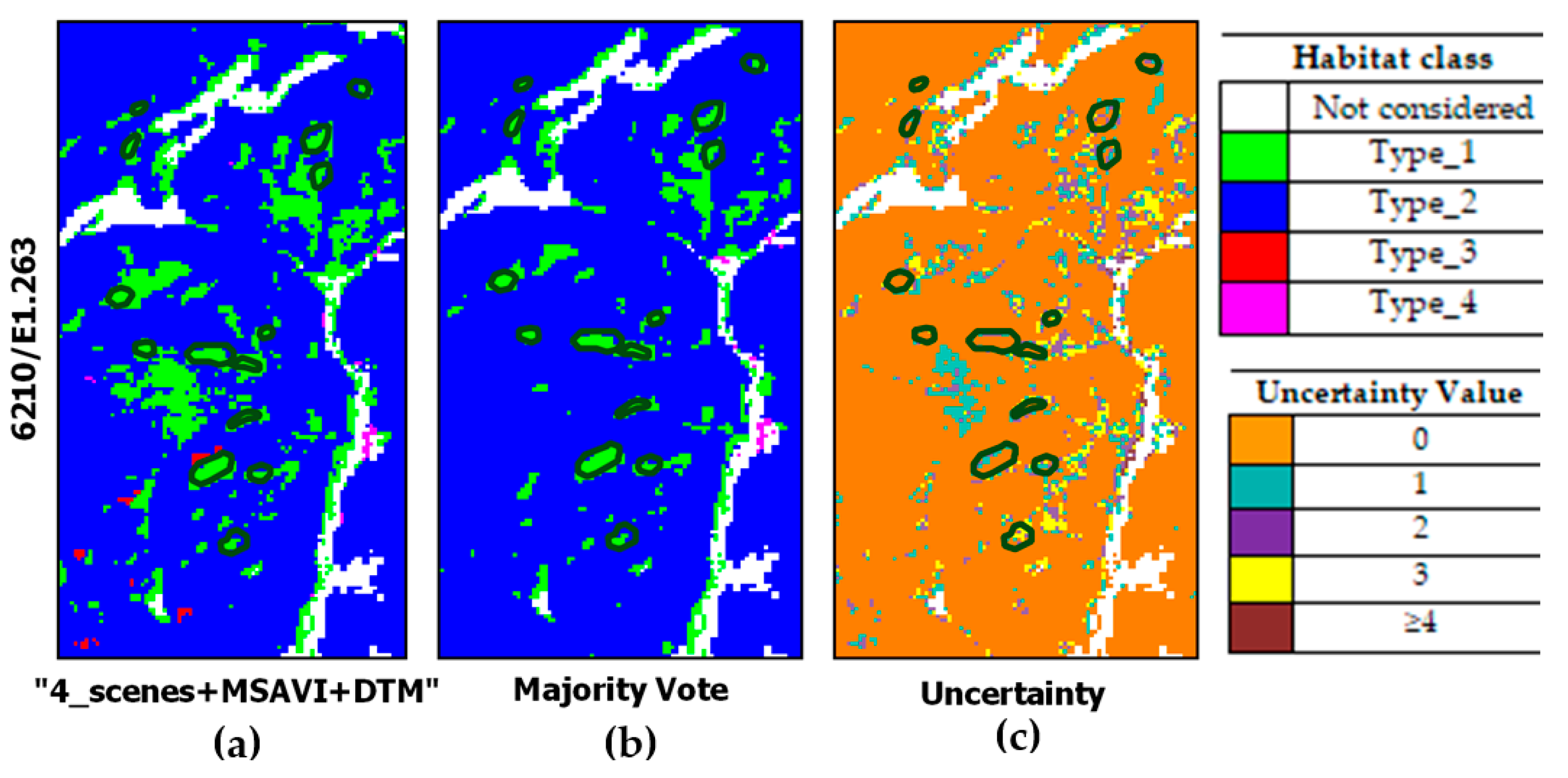
| type_1 | Semi-natural and natural dry grasslands and scrubland facies on calcareous substrates (Festuco-Brometalia). In Murgia Alta, this habitat type is represented by Brachypodium rupestre communities which are attributable both to the Brometalia erecti order and to the Festuco valesiacae-Brometea erecti class. This habitat has been reduced to little patches that can be located in areas found at higher quotas, where agriculture and pasture have been abandoned. BP_1 between late May and first half of June. | 6210 (*)/E1.263 where (*) means (important orchid sites) |
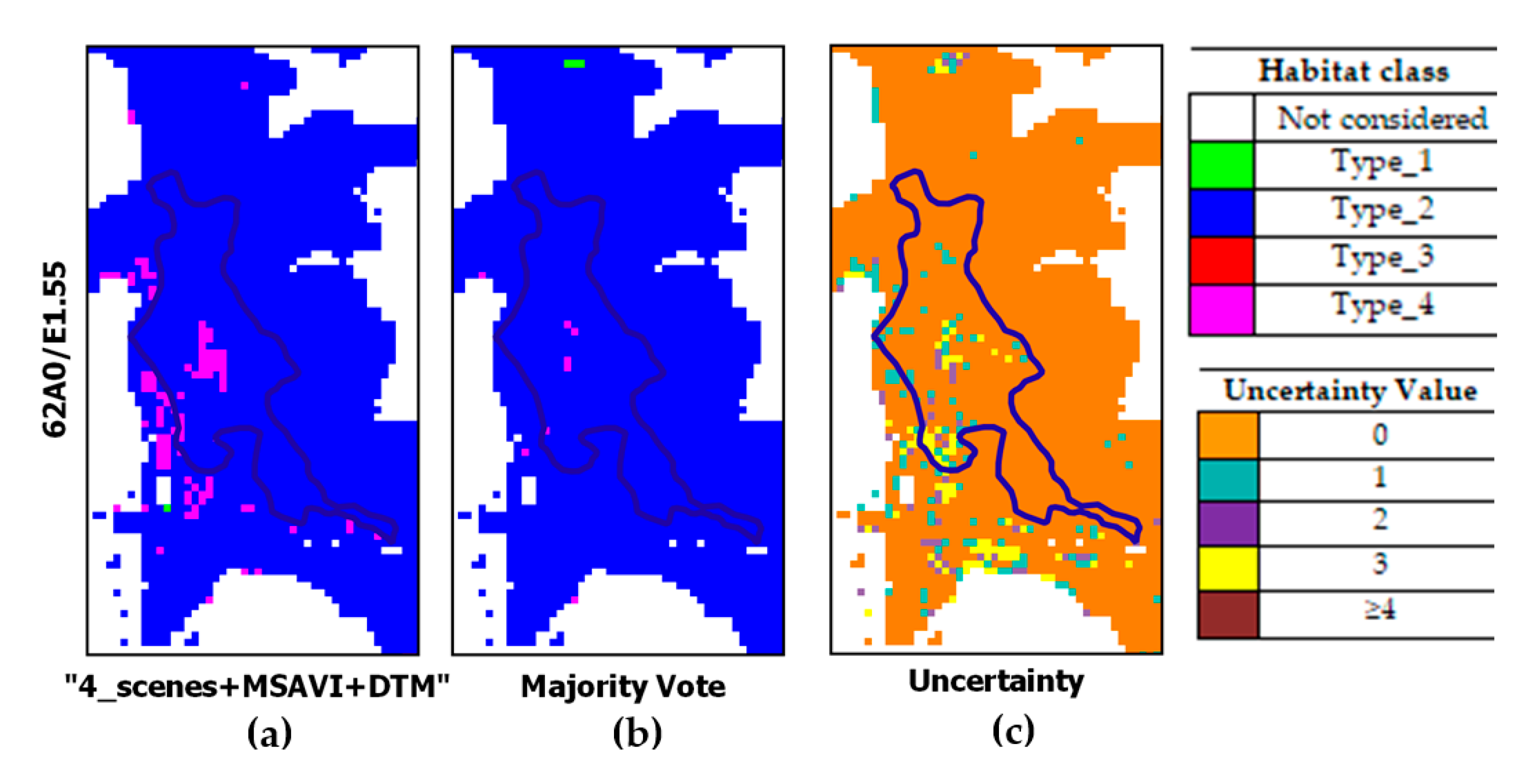
| type_2 | Eastern sub-mediterranean dry grasslands (Scorzoneratalia villosae). This habitat is the most widespread and dominant habitat in the study area and characterized by the endemic feather grass Stipa austroitalica, which constitutes perennial prairies with a rocky nature and relates to the alliance Hippocrepido glaucae-Stipion austroitalicae. BP_2 in May. | 62A0/E1.55 |
| type_3 | Pseudo-steppe with grasses and annuals of the Thero-Brachypodietea. In Murgia Alta, this habitat consists of different types of grasslands, both annual and perennial. Among the annual grasslands are Brachypodium distachyon and Stipellula capensis communities, both referable to the order Brachypodietalia distachyae. Other annual communities resulting aggregated in small patches less than 10 m are not considered in the present study. Among the perennial grasslands are Hyparrhenia hirta and some Ferula communis communities, referable also to the class Lygeo sparti-Stipetea tenacissimae and to the order Hyparrhenietalia hirtae. BP_3 between the second half of April and the beginning of May. | 6220*/E1.434 where * means endemic habitat |
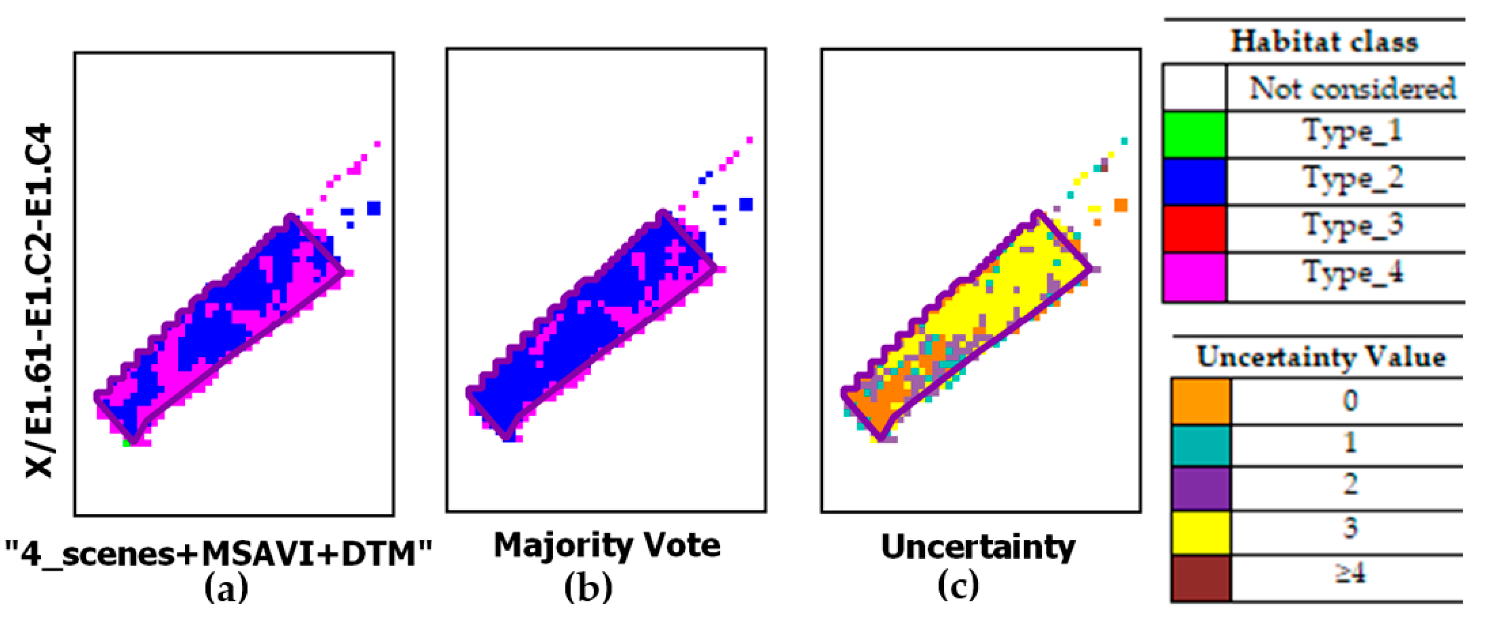
| type_4 | Mediterranean subnitrophilous grass communities, thistle fields and giant fennel (Ferula) stands. In the study area, such grassland type consists of both annual and perennial communities. The annual ones are represented mainly Dasypyrum villosum or Triticum vagans (order Thero-Brometalia; class Stellarietea mediae). The perennial ones, which are both referable to the class Artemisietea vulgaris [52], are represented by Silybum marianum communities (thistle fields) found on overgrazed soils and by Ferula communis communities (giant fennel stands) mostly nitrophilous. These grassland communities can be generally found in lower quota areas. Since these areas are easier to access, they have been cultivated and used for sheep grazing. The listed grassland communities include EUNIS taxonomy codes: E1.61-E1.C2-E1.C4, respectively. BP_4 in the first half of April. | No code in Annex I X/E1.61-E1.C2-E1.C4 |
| Name | Formula | Reference |
|---|---|---|
| GNDVI Green Normalized Difference Vegetation Index | (RNIR(B8) − Rgreen(B3))/(RNIR(B8) + Rgreen(B3)) | [73,74] |
| MSAVI Modified Soil Adjusted Vegetation Index | (2RNIR(B8) + 1 − √(2RNIR(B8) + 1)2 − 8(RNIR(B8) − Rred(B4)))/2 | [74,75] |
| NBR Normalized Burn Ratio | (RNIRnarrow(B8A) − RSWIR(B12))/(RNIRnarrow(B8A) + RSWIR(B12)) | [76,77,78,79] |
| NDRE Normalized Difference Red-Edge | (RNIR(B8A) − Rred-edge1(B5))/(RNIR(B8A) + Rred-edge1(B5)) | [80] |
| REP Red-Edge Position | 705 + 35(((Rred(B4) + Rred-edge3(B7))/2) − Rred − edge1(B5))/(Rred-edge2(B6) + Rred-edge1(B5)) | [81] |
| N° | Input Features Description | Spectral Index | Configuration Acronym |
|---|---|---|---|
| 1 | Stack of 4 multi-season scenes (40 layers): 30 January (biomass pre-peak), 20 April (peak), 19 July (dry season) and 27 October (post-peak), 2018 | “4_scenes” | |
| 2 | Single spectral index time-series (30 layers) | a.MSAVI | “MSAVI” |
| b.GNDVI | “GNDVI” | ||
| c.NBR | “NBR” | ||
| d.NDRE | “NDRE” | ||
| e.REP | “REP” | ||
| 3 | Two spectral indices time-series (60 layers) | a.MSAVI and NBR | “MSAVI+NBR” |
| b.GNDVI and MSAVI | “GNDVI+MSAVI” | ||
| 4 | Three spectral indices time-series (90 layers) | GNDVI, MSAVI and NBR | “GNDVI+MSAVI+NBR” |
| 5 | Three spectral indices time-series with DTM (91 layers) | GNDVI, MSAVI and NBR with DTM | “GNDVI+MSAVI+NBR+DTM” |
| 6 | Stack of 4 multi-season scenes and Single spectral index time-series (70 layers) | Stack of 4 multi-season scenes and MSAVI | “4_scenes+MSAVI” |
| 7 | Stack of 4 multi-season scenes and Single spectral index time-series with DTM (71 layers) | Stack of 4 multi-season scenes and MSAVI with DTM | “4_scenes+MSAVI+DTM” |
| SVM | OA% | UAGRASSLAND% | PAGRASSLAND% | Extension (km2) |
|---|---|---|---|---|
| Binary | 98.16 ± 0.12 | 96.11 ± 0.14 | 98.99 ± 0.07 | 233 |
| Multi-class | 97.79 ± 0.11 | 98.29 ± 0.04 | 99.65 ± 0.03 | 223 |
| N° | Description | FAO-LCCS Code | UA(%) | PA(%) | |
|---|---|---|---|---|---|
| 1 | Cultivated Terrestrial Vegetation/(Trees/Shrubs)Broadleaved.Evergreen | A11/A7.A9 | 89.37 | 84.50 | |
| 2 | Cultivated Terrestrial Vegetation/(Trees/Shrubs)Broadleaved.Deciduous | A11/A7.A10 | 97.86 | 89.46 | |
| 3 | Cultivated Terrestrial Vegetation/Herbaceous | A11/A3 | 98.54 | 96.37 | |
| 4 | C | Natural Terrestrial Vegetation/(Trees/Shrubs)Broadleaved.Deciduous | A12/D1.E2 | 88.03 | 100 |
| 5 | Natural Terrestrial Vegetation/(Trees/Shrubs)Needleleaved.Evergreen | A12/D2.E1 | 99.98 | 99.91 | |
| 6 | Natural Terrestrial Vegetation/Herbaceous (NATURAL GRASSLANDS) | A12/A2 | 98.29 | 99.65 | |
| 7 | Artificial Surfaces/BuiltUp | B15/A1 | 61.51 | 93.37 | |
| 8 | Artificial Surfaces/NonBuiltUp.ExtractionSites | B15/A2.A6 | 96.95 | 100 | |
| 9 | Artificial or Natural Waterbodies/Water | B27-B28/A1.A5 | 100 | 100 | |
| Source | OA% | UAGRASSLAND% | PAGRASSLAND% | Extension (km2) |
|---|---|---|---|---|
| Grassland by SVM | 98.94 ± 0.08 | 98.31 ± 0.07 | 99.60 ± 0.03 | 223 |
| Grassland by CLC | 85.86 ± 2.32 | 87.11 ± 1.70 | 82.44 ± 1.64 | 210 |
| Grassland by Copernicus | 90.59 ± 0.22 | 92.42 ± 0.15 | 88.50 ± 0.16 | 250 |
| Configurations | Habitat | UA% | PA% | F1% | Areamapped (ha) | Areacorrected (ha) |
|---|---|---|---|---|---|---|
| (1) “4_scenes”: OA = 94.80% ± 0.56% | type_1 | 85.46 ± 5.28 | 93.08 ± 3.72 | 89.11 | 2070.89 (+169.43) | 1901.46 ± 136.33 |
| type_2 | 95.68 ± 0.29 | 98.95 ± 0.15 | 97.29 | 19,522.17 (+646.4) | 18,875.77 ± 63.94 | |
| type_3 | 99.28 ± 1.40 | 57.49 ± 3.76 | 72.82 | 289.90 (−210.76) | 500.66 ± 24.39 | |
| type_4 | 96.72 ± 1.76 | 41.23 ± 0.01 | 57.81 | 449.57 (−605.06) | 1054.63 ± 51.49 | |
| (2) “MSAVI”: OA = 94.08% ± 0.48% | type_1 | 79.50 ± 5.61 | 90.39 ± 4.01 | 84.60 | 1418.27 (+170.9) | 1247.37 ± 141.29 |
| type_2 | 95.13 ± 0.31 | 98.14 ± 0.20 | 96.61 | 19,808.83 (+608.10) | 19,200.73 ± 67.35 | |
| type_3 | 94.12 ± 11.53 | 53.65 ± 6.40 | 68.34 | 294.76 (−222.35) | 517.11 ± 76.07 | |
| type_4 | 93.92 ± 2.26 | 55.66 ± 1.48 | 69.90 | 809.66 (−556.65) | 1366.31 ± 71.48 | |
| (3) “MSAVI + NBR”: OA = 93.55% ± 0.56% | type_1 | 77.12 ± 5.37 | 94.02 ± 3.19 | 84.74 | 1893.10 (+340.27) | 1552.83 ± 153.91 |
| type_2 | 96.14 ± 0.28 | 96.17 ± 0.27 | 96.16 | 18,682.38 (+5.12) | 18,677.26 ± 58.41 | |
| type_3 | 84.85 ± 7.10 | 69.73 ± 5.72 | 76.55 | 429.30 (−93.1) | 522.40 ± 103.23 | |
| type_4 | 83.17 ± 2.29 | 69.77 ± 2.36 | 75.88 | 1313.55 (−252.29) | 1565.84 ± 110.23 | |
| (4)“GNDVI + MSAVI + NBR”: OA = 93.97% ± 0.56% | type_1 | 78.60 ± 5.17 | 95.17 ± 2.85 | 86.09 | 2012.46 (+350.32) | 1662.14 ± 152.27 |
| type_2 | 96.72 ± 0.26 | 95.98 ± 0.28 | 97.84 | 18,358.27 (−142.46) | 18,500.73 ± 54.03 | |
| type_3 | 86.11 ± 6.55 | 71.20 ± 5.51 | 77.95 | 422.23 (−88.45) | 510.68 ± 97.79 | |
| type_4 | 83.43 ± 2.73 | 77.42 ± 2.33 | 80.31 | 1539.24 (−119.41) | 1658.65 ± 109.28 | |
| (5)“GNDVI + MSAVI + NBR + DTM”: OA = 94.46% ± 0.53% | type_1 | 86.09 ± 4.48 | 96.15 ± 2.54 | 90.84 | 2085.72 (+218.25) | 1867.46 ± 131.50 |
| type_2 | 96.76 ± 0.26 | 96.41 ± 0.27 | 96.58 | 18,092.50 (−65.64) | 18,158.14 ± 53.79 | |
| type_3 | 80.41 ± 7.94 | 66.88 ± 5.84 | 73.02 | 402.60 (−81.43) | 484.03 ± 110.77 | |
| type_4 | 83.88 ± 2.68 | 80.61 ±2.31 | 82.21 | 1751.57 (−71.19) | 1822.76 ± 108.86 | |
| (6)“4_scenes + MSAVI”: OA = 95.29% ± 0.54% | type_1 | 91.62 ± 3.94 | 95.93 ± 2.76 | 93.73 | 2481.36 (+111.39) | 2369.97 ± 118.17 |
| type_2 | 96.04 ± 0.29 | 98.53 ± 0.18 | 97.27 | 18,514.11 (+467.83) | 18,046.28 ± 60.75 | |
| type_3 | 100 ± 0.01 | 66.63 ± 4.68 | 79.97 | 323.33 (−161.93) | 485.26 ± 0.01 | |
| type_4 | 89.18 ± 2.73 | 63.17 ± 2.09 | 73.95 | 1013.73 (−417.28) | 1431.01 ± 88.80 | |
| (7)“4_scenes + MSAVI + DTM”: OA = 95.45% ± 0.40% | type_1 | 95.21 ± 3.06 | 95.30 ± 2.88 | 95.25 | 1995.18 (+1.89) | 1993.29 ± 78.22 |
| type_2 | 96.31 ± 0.28 | 98.38 ± 0.18 | 97.33 | 18,673.33 (+393.93) | 18,279.40 ± 58.22 | |
| type_3 | 95.93 ± 3.50 | 69.02 ± 4.92 | 80.27 | 350.02 (−136.48) | 486.50 ± 55.61 | |
| type_4 | 83.47 ± 2.98 | 69.71 ± 2.36 | 75.97 | 1314.00 (−259.37) | 1573.37 ± 109.27 |
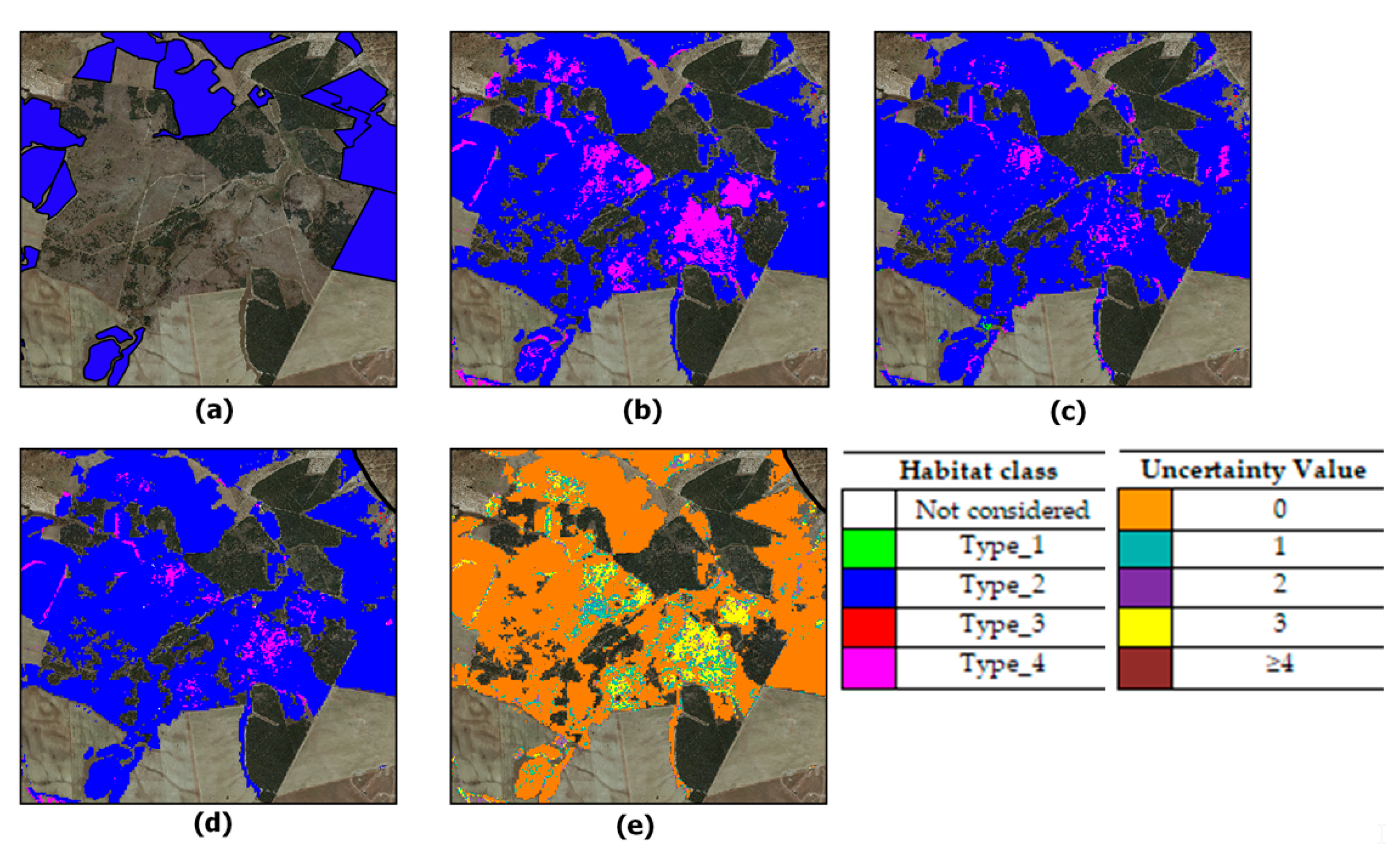
| N° Classifiers Considered | Uncertainty | N° Validation Pixels | OA% |
|---|---|---|---|
| ≤3 | ≥4 | 12 | - |
| 4 | 3 | 304 | 47.70 |
| 5 | 2 | 264 | 59.85 |
| 6 | 1 | 353 | 77.05 |
| 7 | 0 | 18,007 | 97.43 |
| Area (ha) | ||||
|---|---|---|---|---|
| Type_1 | Type_2 | Type_3 | Type_4 | |
| MV | 1718.76 | 19185.56 | 322.27 | 902.06 |
| “4_scenes+MSAVI+DTM” | 1995.18 | 18673.33 | 350.02 | 1314.00 |
Publisher’s Note: MDPI stays neutral with regard to jurisdictional claims in published maps and institutional affiliations. |
© 2021 by the authors. Licensee MDPI, Basel, Switzerland. This article is an open access article distributed under the terms and conditions of the Creative Commons Attribution (CC BY) license (http://creativecommons.org/licenses/by/4.0/).
Share and Cite
Tarantino, C.; Forte, L.; Blonda, P.; Vicario, S.; Tomaselli, V.; Beierkuhnlein, C.; Adamo, M. Intra-Annual Sentinel-2 Time-Series Supporting Grassland Habitat Discrimination. Remote Sens. 2021, 13, 277. https://0-doi-org.brum.beds.ac.uk/10.3390/rs13020277
Tarantino C, Forte L, Blonda P, Vicario S, Tomaselli V, Beierkuhnlein C, Adamo M. Intra-Annual Sentinel-2 Time-Series Supporting Grassland Habitat Discrimination. Remote Sensing. 2021; 13(2):277. https://0-doi-org.brum.beds.ac.uk/10.3390/rs13020277
Chicago/Turabian StyleTarantino, Cristina, Luigi Forte, Palma Blonda, Saverio Vicario, Valeria Tomaselli, Carl Beierkuhnlein, and Maria Adamo. 2021. "Intra-Annual Sentinel-2 Time-Series Supporting Grassland Habitat Discrimination" Remote Sensing 13, no. 2: 277. https://0-doi-org.brum.beds.ac.uk/10.3390/rs13020277