Mapping Seasonal Agricultural Land Use Types Using Deep Learning on Sentinel-2 Image Time Series


Norwegian Institute of Bioeconomy Research (NIBIO), P.O. Box 115, 1431 Ås, Norway
*
Author to whom correspondence should be addressed.
Remote Sens. 2021, 13(2), 289; https://0-doi-org.brum.beds.ac.uk/10.3390/rs13020289
Submission received: 11 December 2020
/
Revised: 6 January 2021
/
Accepted: 12 January 2021
/
Published: 15 January 2021
(This article belongs to the Collection Sentinel-2: Science and Applications)
Abstract
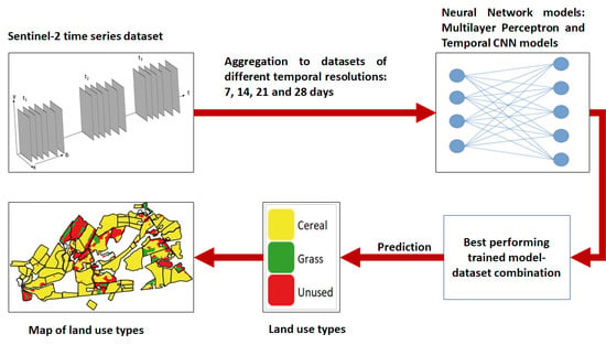
:The size and location of agricultural fields that are in active use and the type of use during the growing season are among the vital information that is needed for the careful planning and forecasting of agricultural production at national and regional scales. In areas where such data are not readily available, an independent seasonal monitoring method is needed. Remote sensing is a widely used tool to map land use types, although there are some limitations that can partly be circumvented by using, among others, multiple observations, careful feature selection and appropriate analysis methods. Here, we used Sentinel-2 satellite image time series (SITS) over the land area of Norway to map three agricultural land use classes: cereal crops, fodder crops (grass) and unused areas. The Multilayer Perceptron (MLP) and two variants of the Convolutional Neural Network (CNN), are implemented on SITS data of four different temporal resolutions. These enabled us to compare twelve model-dataset combinations to identify the model-dataset combination that results in the most accurate predictions. The CNN is implemented in the spectral and temporal dimensions instead of the conventional spatial dimension. Rather than using existing deep learning architectures, an autotuning procedure is implemented so that the model hyperparameters are empirically optimized during the training. The results obtained on held-out test data show that up to 94 % overall accuracy and 90% Cohen’s Kappa can be obtained when the 2D CNN is applied on the SITS data with a temporal resolution of 7 days. This is closely followed by the 1D CNN on the same dataset. However, the latter performs better than the former in predicting data outside the training set. It is further observed that cereal is predicted with the highest accuracy, followed by grass. Predicting the unused areas has been found to be difficult as there is no distinct surface condition that is common for all unused areas.
1. Introduction
There is a consensus that modern agricultural production is expected to happen within the requirements of sustainability and climate change [1,2]. This demands careful planning and precise forecasting of agricultural production, which rely on up-to-date, detailed and accurate information about agricultural land use [3,4]. The size and location of agricultural fields in active use and the type of use they are utilized for during each growing season is among the vital information needed. Equally important is the size and location of agricultural fields that are unused during a growing season. These areas are either temporarily or permanently out of food and fodder production. According to national agricultural policy in Norway, it is a goal to increase food production by 20 percent within 2030. To achieve this goal, it is necessary to maintain agricultural fields for food production.
Monitoring agricultural fields in practice is, however, a demanding task. Some countries have detailed land information system at the level of parcels, for, e.g., The Netherlands [5], where annual monitoring can be conducted through parcel registration. The basic map unit in Norway, on the other hand, is the property map, while detailed maps at parcel level do not exist. Annual uses of agricultural areas are registered only through farmers’ applications for a national agricultural subsidy. Each farmer reports the size of the land in use and for which purpose it is used without linking it to a specific parcel or field. The data that is registered are, therefore, non-spatial. As these data are tied to subsidy benefits, the certainty of the registered data is at least questionable. Ideally, an independent system of permanent parcel delineation and annual monitoring is beneficial to land use planning, production forecasting and subsidy estimation. In the absence of such a system, an independent annual monitoring of agricultural land uses is a feasible alternative.
At the forefront of the list of tools used for agricultural monitoring is remote sensing. Remote sensing has long been used in agriculture for various purposes. Some examples of use cases are mapping agricultural land use and crop types [6,7], monitoring agricultural activities and crop growth [8], forecasting yields [9], and detection of diseases [10]. Although not exhaustive, these application examples demonstrate the use of remote sensing as a tool for inventory, monitoring and forecasting agricultural production. However, there are a few limitations caused by the characteristics of the data and the methods of analysis. The low spatial resolutions of most publicly available remote sensing images often fail to fulfill the required spatial precision in fragmented agricultural fields. Weather conditions, at least for optical images, and low temporal resolution, limit the opportunities to obtain good quality data over a given period. The characteristically large data volume of remote sensing also continues to be a challenge.
The past few years have, however, seen major improvements in the technologies for acquiring, storing and analyzing remote sensing data. The spectral, spatial and temporal characteristics of remote sensing images have generally improved. A few satellites, both commercial and public, with high spatial resolution, have been launched. The Sentinel-2 optical satellites of the European Union’s Earth Observation Program called Copernicus collect data over the entire globe in 13 spectral bands, with a spatial resolution ranging between 10 and 60 m [11]. They repeat the imaging process every 5 days at the equator and on even fewer days towards the poles. The high temporal resolution increases the chances of acquiring data on cloud-free days or mosaicking cloud free images over a relatively short period. It also adds a temporal dimension that can improve pattern recognition problems such as land cover classification.
Image-processing tools and algorithms have also improved over the past years. The improvements in big data and machine learning technologies are among the most important. Artificial Neural Network (ANN), although developed many decades ago, has evolved into a leading practical machine learning tool relatively recently, as a result of the exponential increase in computational capabilities and the availability of training data [12]. Among the many machine learning algorithms developed based on ANN, Multilayer Perceptron (MLP) [13], Convolutional Neural Network (CNN) [14], Recurrent Neural Network (RNN) [15], etc., are the most common examples. There is rich coverage from the literature on each of the algorithms and their numerous variants [16,17]. These ANN-based algorithms have proven to be effective alternatives to traditional statistical methods, especially for complex and nonlinear problems, as they are non-parametric and assume no prior statistical distribution of the data [16]. The algorithms can be built in such a way that they take layer upon layer of variants of neural networks depending on the complexity of the data and the problem they handle. Deep learning is the phrase used to describe these multilayer neural networks [12].
Deep learning is used in remote sensing for various applications [18], image classification being one. Any of the deep learning models can be adapted for image classification depending on the characteristics of the data and the purpose of classification. Often, due to the complexity of the problem and the higher precision needed for the classification result, remotely sensed data from a point in time is not enough, even with the use of deep learning. Data over longer timespans, hence time series, can capture the temporal pattern that manifests differently for different classes of objects. Time series classification deals with assigning a label (class) to unlabeled time series data using a trained model from labeled training samples. Detailed reviews of methods used in time series classification, including deep learning, are available [19] and will not be discussed here. MLP is often used when one chooses to ignore the temporal dimension and treat the time series as independent multivariate data. The MLP has been applied to optical and SAR images to classify seasonal crops in Ukraine [20]. MLP has also been used to estimate sorghum biomass production from image time series acquired by an Unmanned Aerial Vehicle (UAV) [21]. In both cases, the temporal and the spectral orders of the data are not fully utilized. The time dimension is considered in cases where, for example, RNN is used for time series classification [22]. However, [19] state that RNN is more suited to forecasting problems than classification. Among the limitations summarized by [19] are that RNN: 1) suffers from a vanishing gradient problem, 2) is hard to train due to difficulties in parallelizing, 3) is computationally demanding as it relies on the total history as opposed to the CNN which learns from time windows. As a result, CNN is gaining popularity for time series classification. CNN is, in some cases, used with a 1D kernel along the temporal dimension, as demonstrated in [23,24]. 3D CNN is also implemented to include the temporal dimension as a third dimension, as, for example, used by [25] for crop classification using multitemporal satellite images. 3D CNN involves convolution over the spatial dimensions, and the order of the spectral bands is not utilized. As a spatial window is used for the convolution, pixels are not evaluated independently.
Recently a comprehensive contribution proposed a temporal CNN architecture by demonstrating its application on Formosat-2 image time series [26]. In the study, CNN is applied using kernels along the temporal and spectral dimensions turn by turn (1D) and simultaneously (2D) investigating the contribution of each dimension. The proposed temporal CNN architecture opens an interesting methodological option that needs further testing and application on other images and application areas. The spatial and temporal resolutions of the Formsat-2 [27] are different from the currently widely used satellites, for example, Sentinel-2 [11]. In conventional CNN, convolution is carried out in the spatial dimensions to make use of the spatial texture variations. The use of 2D CNN based on spatial dimension alone, as satellite remote sensing has limitations. This is partly due to the fact that the spatial features of land use types are not as distinct as often seen in ordinary object classes such as cats and dogs, widely used as examples in machine learning. Additionally, when spatial kernels are used for convolution, pixels are not evaluated independently of their adjacent pixels. This has implications for large pixels, as in the case of satellite images, and pixels at the boundaries of fields and at image edges. Enhancing a pixel into an image by using the spectral and temporal dimensions instead of the spatial dimension enables independent evaluation of a pixel. Temporal changes in land surface manifest differently for different land use types and indicate the usefulness of the temporal dimension in pattern classification, similar to the spectral dimension.
This paper presents an application of deep learning algorithms and satellite image time series (SITS) data from Sentinel-2 to map and monitor agricultural land use in Norway. The spectral–temporal differences in the different land use types are explored first. The study then investigates the applicability of temporal CNNs for mapping the major agricultural land use types: cereal crops, fodder crops (grasses), and land left out of production. The relatively simple MLP algorithm is tested and used as a baseline to evaluate the more complex CNN algorithms. We have optimized different variants of the deep learning models to identify the most suitable model for mapping land use types. Norway often has cloudy weather and missing observations that need to be addressed with interpolation. The research therefore investigates which temporal resolution of the Sentinel-2 SITS data, aggregated and interpolated for missing data, is most suitable for the objective stated in regions of frequent cloud coverage. The best performing model–dataset combination is then used to map and evaluate seasonal agricultural land uses. The results have implications for the seasonal monitoring of agricultural land uses in the absence of alternative methods.
2. Materials and Methods
2.1. Data
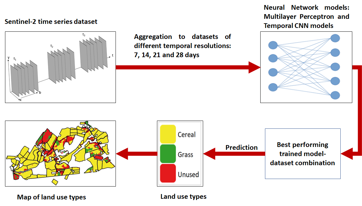
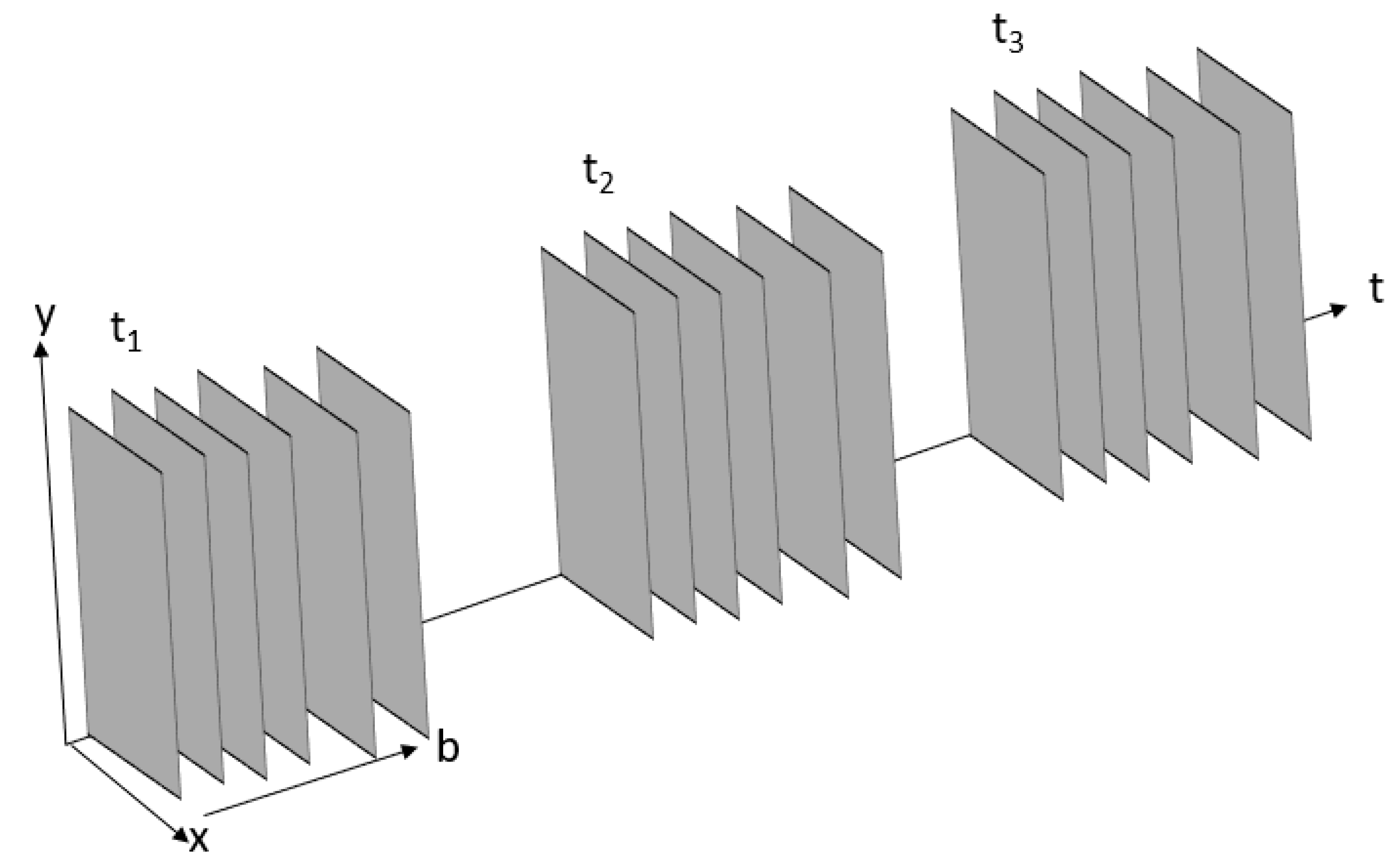
The Sentinel-2 images acquired during the period between the 15th of April and the 15th of October 2019 over the land area of Norway are downloaded and organized as a data cube in a NetCDF-4 format. As the land use types can change from year to year, we decided to use data from a single year, i.e., 2019. The year is selected as it is the most recent year for which training data were accessible. Six bands of the atmospherically corrected images (level 2A), namely the three visible (bands 2, 3 and 4), the near infrared (band 8A), and the two middle infrared bands (bands 11 and 12) are selected. The classification layer created during the atmospheric correction is also included for later masking of clouds and shadows. The bands are resampled to 20 m pixel size to reduce the data volume and the effect of georeferencing error. The satellite image time series (SITS) data are then stored tile by tile for the entire land area of the country in a data model represented in Figure 1.
Three agricultural land use classes are defined, namely: (1) Cereal, representing areas used for cultivation of cereals such as wheat, barley, rye, and oat; (2) Grass, representing areas used for the cultivation of grass-based fodder; (3) Unused, representing agricultural areas without crops, i.e., temporarily or permanently abandoned with activities not qualifying for subsidies.
Training data for each of the three classes are collected manually using the production subsidy (PT) database together with the property map. Some farmers have small farms, and they produce either cereals or grass on their farm. A farmer applies for a subsidy annually, and the production data for each farm are stored in the PT database. In this way, the production subsidy data are linked to the property map. In cases where it is difficult to establish a spatial connection between production reports and property maps, the farms are not represented in the training dataset. Such cases arise where a farmer reports that some part of his/her farm is in use for food and fodder crops while the rest is not, or some part is used for cereal crops while the rest is used for fodder grass. The unused class could not be obtained directly from the PT database. However, a year when a farmer has not applied for subsidy at all is an indication that the farm is not used for crop production, i.e., is unused. The training data used for further analysis are collected by picking three random points from each of the identified polygons.
The training points gathered in the above process contain the location data and the land use status. The values of the SITS data at the training points are extracted from the NetCDF files. After the extraction, every point has values for each band for each timestamp. In some cases, there are missing data due to the masking of clouds and shadows. In such cases, the values are interpolated from the two closest timestamps using linear interpolation. The training data are, thereafter, complete with the spectral data and the land use classes. About 43,000 training points are collected scattered throughout the country. The training data are further aggregated into different time steps, as discussed below.
2.2. Conceptualization of the SITS Data for Machine Learning
Let us assume time series as T = t1, t2, t3, …, tt, where subscripts 1…t stand for timestamps. In SITS, the time intervals are not uniform unless one is collecting data from only one orbital path without any filtering. This means that the time gap between t1 and t2 is not necessarily equal to the time gap between t2 and t3, and so forth. Additionally, optical satellite images are often affected by weather conditions. Therefore, there is a need for feature selection or feature extraction. The SITS data with size t are reduced to SITS data with size n, n being less than t, resulting in T = t1, t2, t3, …, tn. This reduces the data size, makes the time interval uniform and reduces noise (e.g., clouds and shadows). The temporal interval, sometimes called a window, to be used is chosen purposely. For this study, we used 7, 14, 21 and 28 days, respectively, representing from a week to a month. The temporal intervals are chosen for convenience in overlapping with multiples of week, as the temporal resolution of the Sentinel-2 is not constant for the entire country. Due to increasing overlaps between swaths of adjacent orbits with increasing latitude, the temporal frequency is higher over Norway than the nominal 5 days. As a result, the frequency over Norway varies from south to north. We selected a minimum interval of seven days to include multiple acquisitions for each location. The aggregation technique to map from t size data to n size data depends on the type of the time series data. To reduce the effects of shadows (low digital values) and clouds (high digital values), common in raw optical satellite data, the median statistic is preferred in this study. For the time steps lacking image data, the values are interpolated from the nearest time steps using linear interpolation method. Linear interpolation is a commonly known algorithm used for filling missing values in time series images, and is suitable when global smoothing is not attractive [28]. Missing data in satellite images are often related to cloud cover, where adjacent pixels are missing at the same time. Therefore, in this case, temporal interpolation is more practical and preferred over spatial interpolation. The dataset then becomes a 4D array of two spatial dimensions representing the northings and eastings, with one dimension representing the spectral bands of the Sentinel-2 and one dimension representing the time steps chosen.
The analysis of the SITS data is approached based on the following three different conceptualizations:
(1) The image data for each band at each time are treated as an independent predictor variable. The data are not treated as time series but as a multivariate dataset, with multiple independent variables and a dependent variable. The number of the independent variables is equal to the number of bands multiplied by the number of time steps. The goal is then to train a model that relates the predictor variables to the dependent variable, the land use classes in this case, so that the model can be used to classify the scenes;
(2) The image data over the time periods are treated as a one-dimensional time series. That is, a pixel is assumed to be observed using each band alternatively over the time period. The spectral bands are treated as independent, whereas the temporal dimension is treated as a continuous series of temporal data. Temporal features of the spectral data can then be extracted to model the land use classes;
(3) Assigning one dimension to the time variable and another to the spectral bands, the observation at a pixel can be treated as a 2D representation of the pixel over temporal and spectral dimensions. Here, both the time order and the spectral order are important, together giving a 2D perspective of data collected at a point in space, i.e., a pixel. Both temporal, spectral and spectral–temporal features can be extracted by treating these 2D data as an entity, just like an image of a cat or any other object.
2.3. Implementation of the Deep Learning Algorithms
2.3.1. Preprocessing
The training data represent six spectral bands collected over the time period specified above. After aggregating the training data to a defined temporal resolution, the data are rescaled to values between 0 and 1 using the MinMax scaler of Scikit-learn preprocessing Python package (v. 0.23.2., [29]). The data are then split into a training (70%) and a test (30%) set through random selection. The test dataset is kept out of the training process for later evaluation of the trained models.
2.3.2. Model Selection and Training
Python API of the Keras package, built on top of the Google-developed machine learning program called Tensorflow (v. 2.1.0, [30]), is used. To implement a machine learning scheme, one needs to select a model and the model parameters. Variants of two ANN-based machine learning models, namely the MLP and the CNN, are selected based on the conceptualizations discussed above. Model parameters are of two types: trainable parameters that are learned during training, and the hyperparameters that are defined manually or fine-tuned automatically. The trainable parameters are mostly the weights and biases of the model, whereas there is a long list of hyperparameters depending on the type of model used.
The MLP model is widely applied to multivariate data fitting into the first conceptualization, defined above. The MLP models the relationship between predictor variables and a dependent variable by estimating the probability that a pixel or a record belongs to a class. The probability is a weighted sum of the predictor variables converted to probability using a certain function, e.g., SoftMax [31]. The weights and the accompanying biases are estimated through iteration with the objective of minimizing a defined loss function. In search of an accurate model, layer upon layer of the neural net can be used, where the outputs of one layer are fed as input to the next layer. The output of the final layer is fed to the function that translates it into probability values. Mathematical details of deep learning architectures are given in the literature (e.g., [32,33]) and will not be discussed further here.
The MLP has a few hyperparameters whose values need to be set before the training. Optimizing the hyperparameters is not an easy task. Manual trial-and-error approaches are impractical for going through all the value domains. Therefore, an automated method of hyperparameter tuning is implemented using Keras tuner [34]. The Keras tuner is a package that automatically goes through the different value combinations of the hyperparameters, and trains each combination, and evaluates and compares them based on a criterium set by the user, for example, the validation accuracy. The first step in optimizing the hyperparameters is defining the domains of each of the parameters. Traversing through the theoretical domains is practically impossible, as some of the parameters have an infinite domain. The practical domain (parameter space) can, therefore, be defined in a trial-and-error approach to obtain the threshold values beyond which the performances of the algorithm declines. Even after defining the parameter space, a brute-force approach of going through all possible combinations of the values is computationally demanding. Fortunately, the Keras tuner provides a system which selects a defined number of models whose parameter values are combined randomly, i.e., randomized search. Here, the randomized search method is applied with the parameter domains presented in Table 1 below.
Variants of the CNN algorithm are implemented for the second and the third data conceptualization, shown above. Where only the temporal order is considered important, i.e., in the second conceptualization shown above, a CNN architecture that convolves the data with a 1D kernel along the temporal dimension, extraction features that are expressive of the temporal variation of the values, is implemented. Where the data are conceptualized as 2D data, with the spectral and temporal dimensions taking one dimension each, a 2D CNN algorithm is implemented. A 2D (along the spectral and temporal dimensions) kernel is then used to convolve the data to extract various features. This enables the convolution to be performed on a single pixel rather than on a set of adjacent pixels. Each pixel is treated as an image, as opposed to the spatial CNN, where an image is a set of adjacent pixels. A CNN architecture is defined based on the number and size of hyperparameters. The number of trainable parameters is dependent on the hyperparameters. Instead of using one of the available CNN architectures, the architecture is built through autotuning the different hyperparameters for both the 1D and the 2D CNN. Here, the randomized search of the Keras tuner module is also used after defining the search space of the hyperparameters as presented in Table 1.
In Figure 2, an example architecture of the 2D CNN model, based on the spectral and temporal dimensions, is presented. It is a simple architecture with two hidden layers. In most CNN implementations, convolution is followed by other steps (not included in the figure) that help the model to generalize better, for example pooling and dropout. The figure does not propose a new architecture; it is instead used to show how the spectral and temporal dimensions are used in the input layer. The input image depicted in the figure is a single pixel converted to an image using its temporal and spectral dimensions. The size of the spectral dimension is six, whereas the size of the dimensions varies depending on the temporal interval used. The kernel of size three by three refers to length of three in both the temporal and the spectral dimensions. The pixel is then convolved consecutively depending on the number of the hidden layers. The final convolution is flattened, and a fully connected network is then applied. Finally, the SoftMax function converts the final output to probability values for each of the classes. A batch of such pixel images are fed into the model during training and prediction.
2.3.3. Dealing with Overfitting
One of the challenges of machine learning is the tendency of the models to try to perfectly fit the training data, i.e., overfitting, instead of generalizing it. Overfit models fail to predict samples outside the training set with the same level of accuracy. To deal with overfitting of the models, some measures were taken, namely, dropout [35], batch normalization [36], regularization (both L1 and L2) [37], data augmentation [38] and early stopping. The dropout process removes a certain fraction of features, those with the lowest weights, in every layer. This forces the training to adapt more to the features with high weights. Batch normalization is important to rescale the inputs of the hidden layers and speed up the learning process. Although we rescale the input layer, there is a problem of value shift in the resulting features. Weight regularization penalizes the outliers, basically high-weight features, so that the model generalizes better. The dropout rate and the weight regularizations are optimized through the hyperparameter-tuning process. Additionally, to virtually increase the sample size and to generalize better, data augmentation is implemented. As in data orientation, temporal versus spectral is important and must be kept rigid, so no rotation, translation and shearing are implemented. The presence of noise is more realistic in this study. Therefore, in data augmentation, only spectral transformation using a gaussian noise of mean 0 and variance 0.03 is implemented. Early stopping is also implemented in such a way that the trends in the validation loss are monitored, and the training stops when the validation loss keeps on increasing for a certain number of consecutive epochs. Further training beyond this epoch leads to overfitting.
2.3.4. Testing of the Trained Models
As stated above, four temporal datasets were used based on four different temporal resolutions. Their comparison helps understand which temporal interval is suitable for time series analysis of Sentinel-2 images in cloudy regions such as Norway. The four temporal datasets were tested on three different deep learning models, namely MLP, 1D CNN and 2D CNN. As a result, twelve sets of model–dataset combinations were compared. The hyperparameters of the models were tuned using the randomized search method of the Keras tuner by limiting the number of the randomly selected models to 20 for each of the twelve combinations. One optimized model was selected for each of the twelve model–dataset combinations based on the validation accuracy from 20% of the training data. The optimized models were then compared to each other based on the accuracy with which the test classes were predicted, using overall accuracy and Cohen’s Kappa.
2.3.5. Prediction and Evaluation
Machine learning models often fail to predict with the same level of accuracy that they train with. Therefore, before deciding which model is best, a prediction is made for areas that have independent field observations. As the test data are collected under the same conditions as the data used for the training, a totally independent dataset is needed. Such data were obtained from two sources. The first source was the Norwegian Agricultural Environmental Monitoring Programme (JOVA). JOVA is a national monitoring programme for nutrient runoff from agricultural fields which consists of 13 sites across Norway where several environmental variables are monitored together with detailed information on agricultural practice on a parcel level. For this study, only one such site of 43 hectare was available, with data from 2019. The second approach was the manual collection of additional data using the PT database and the property map in a similar approach to the ones collected for the training, but this time using the entire polygons rather than selecting a few points.
We predicted the land use classes using twelve different optimized models for areas that have field-recorded data. To remove salt-and-paper type noise from the predicted maps, we used a majority filter of a three by three window. The field data from JOVA and PT were then compared to the predicted land use maps, and the numbers of agreeing and disagreeing pixels were counted. We computed the accuracies of the predictions based on the overall accuracy, precision, recall and F1 score [39]. The model–dataset combination that produced the highest accuracy was used for the final prediction of the land use classes for the entire county.
3. Results
3.1. Typical Temporal Signatures of the Three Land Use Status
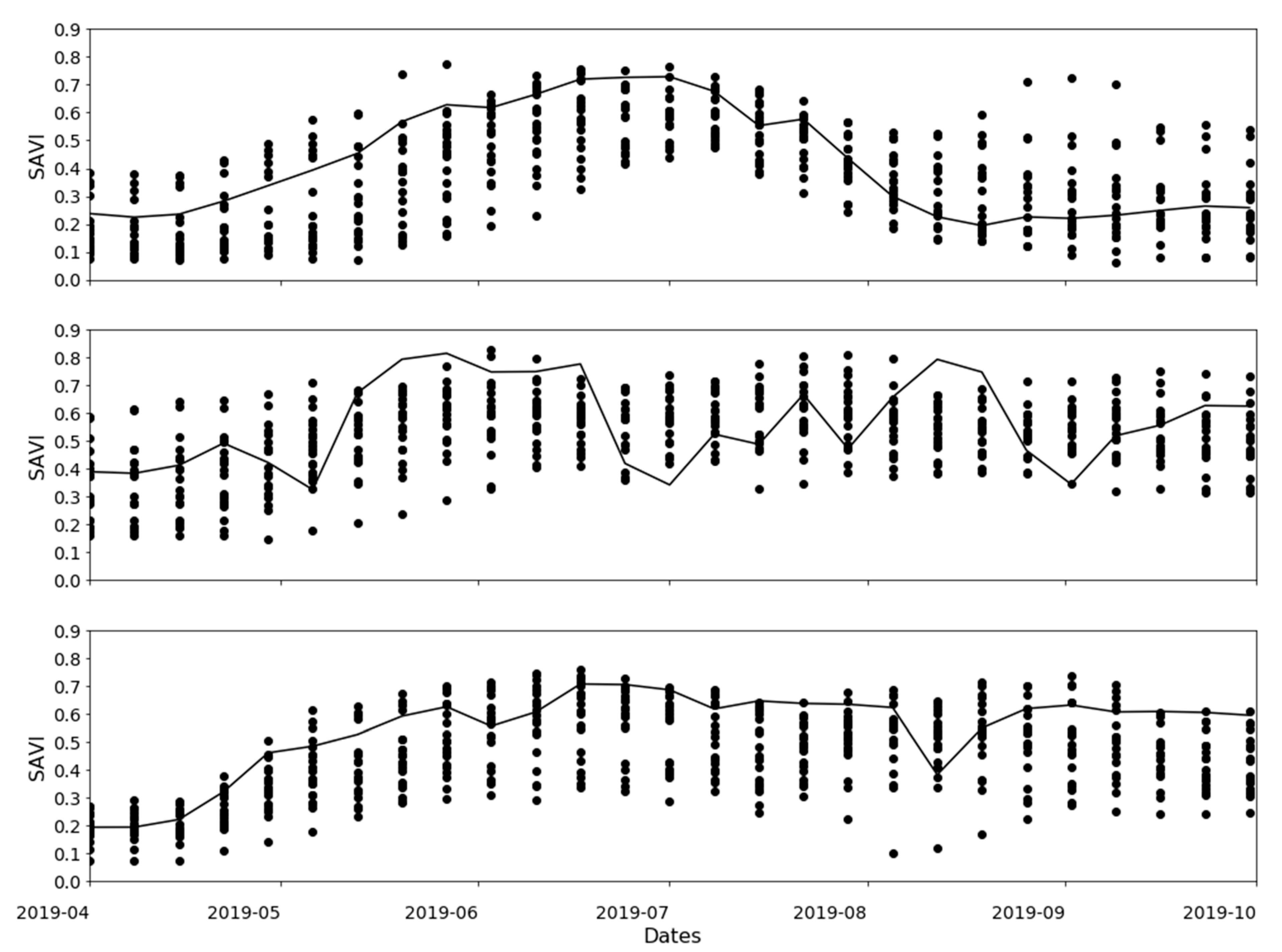
The basis of classifying land uses from remotely sensed data is the spectral differences between the classes. Similarly, the use of SITS entails differences in both spectral and temporal signatures between the different classes. Although there is no need to present the entire exploratory analysis of the spectral–temporal signatures of the different land uses, Figure 3 presents the temporal signatures of the Soil Adjusted Vegetation Index (SAVI [40]) of the three different land use classes as an example. Although SAVI is not used directly as an input in the models, it is useful to visualize the temporal differences between the three classes. Here, the pixels that are considered representative of each class are selected. Cereal shows a typical bell-shaped curve, while grass shows multiple drops starting from the beginning of July. On the other hand, the example for unused is taken from a pasture, and this curve has a high value throughout the growing season. The slight drop in middle of August is probably an artefact caused by an observation affected by a cloud or cloud shadow not being labelled correctly in the L2A product.
3.2. The Optimized Models and Their Hyperparameters
The specifications of the optimized model for each of the twelve model–dataset combinations are presented in Table 2. As can be seen from the table, some hyperparameter values do not have a specific relationship with the model type or the dataset type. However, the highest number of hidden layers that produced a good result is four. Increasing the number of hidden layers does not improve accuracy for the MLP, as two or three hidden layers performed best. For the CNN algorithms, the optimum number of filters and the filter size increases when 1D CNN is used as opposed to the 2D CNN, whereas, the optimum rate of dropout has an opposite trend. The activation function that resulted in the best fitting model was consistently found to be the ReLU function. The table also shows that the optimum values of the parameters change with the model type rather than with the dataset type, i.e., temporal resolution.
3.3. Performances of the Model–Dataset Combinations on the Test Dataset
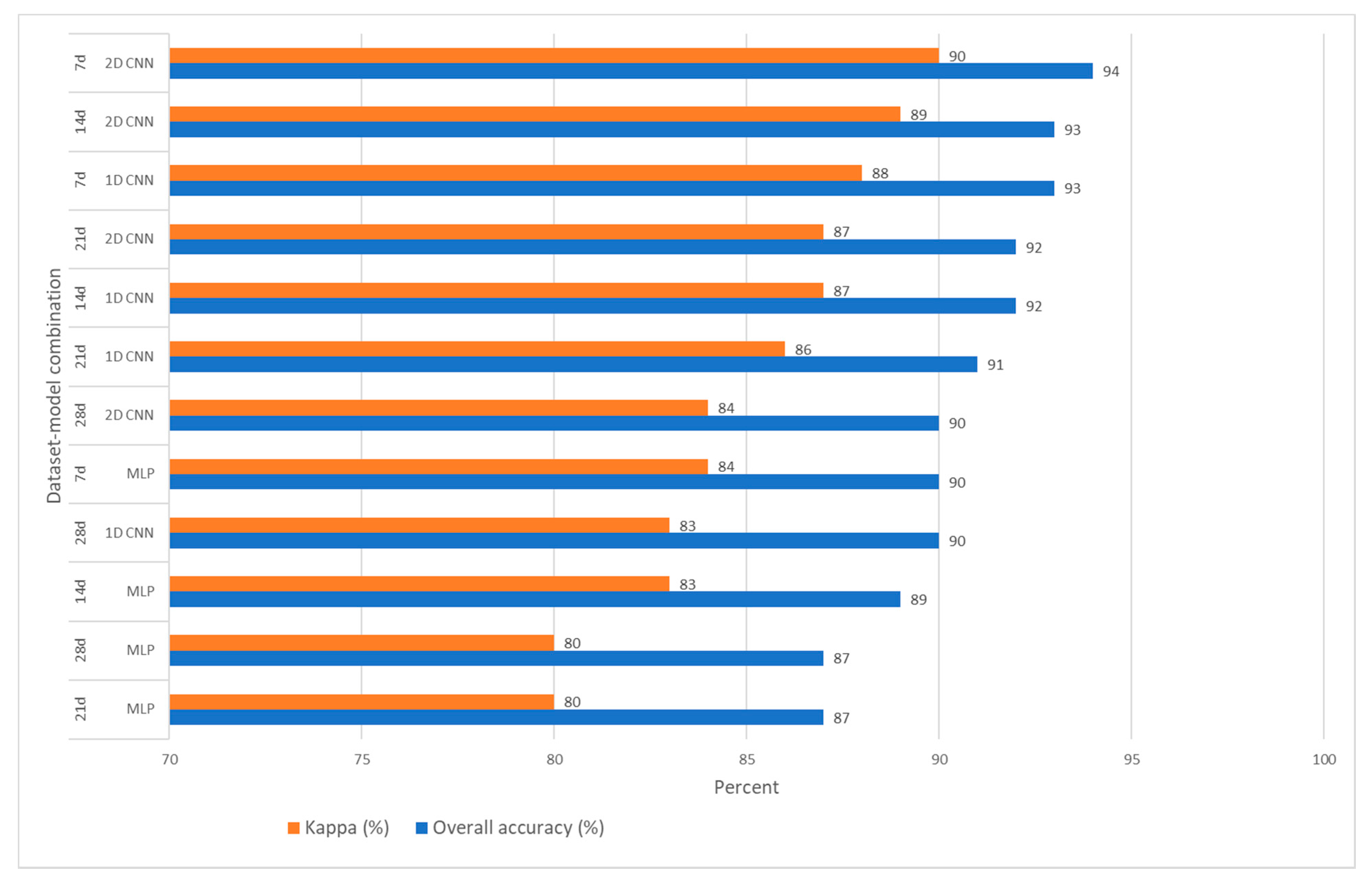
The accuracy measures of the test data for the twelve model–dataset combinations are presented in Figure 4. As can be seen from the figure in all accuracy measures, the 2D CNN model trained on the SITS data with a 7 days temporal interval performed best, with an overall accuracy of 94% and a Cohen’s Kappa of 90%. This is followed by 1D CNN, applied on the SITS data with 7 days temporal interval, and 2D CNN, applied on the SITS data with 14 days temporal interval, performing roughly equally. The worst accuracy was obtained when the MLP algorithm was applied on the SITS data with 28 days temporal interval. The values were obtained based on the optimized model applied on the held-out test datasets.
Overall observation of the performances, i.e., overall accuracy and Cohen’s Kappa, of the models and the datasets, shows that the 2D CNN performs best compared to the other two models, and the 7 days temporal resolution performs best compared to the other temporal resolutions. The overall accuracy gains of using the 7 days data over the 28 days data is about 4%, whereas the overall accuracy gains of using 2D CNN over the 1D CNN and the MLP is roughly 1% and 5%, respectively, as can be deduced from the figure. The detailed accuracy parameters of the 2D CNN implemented on the dataset with a temporal resolution of 7 days is presented in Table 3. The precision, recall, F1 score and other accuracy measures are presented, as an example, to show that the models performed almost similarly on the three different classes, although the sample sizes are unbalanced.
3.4. Prediction and Evaluation of the Model-Dataset Combinations
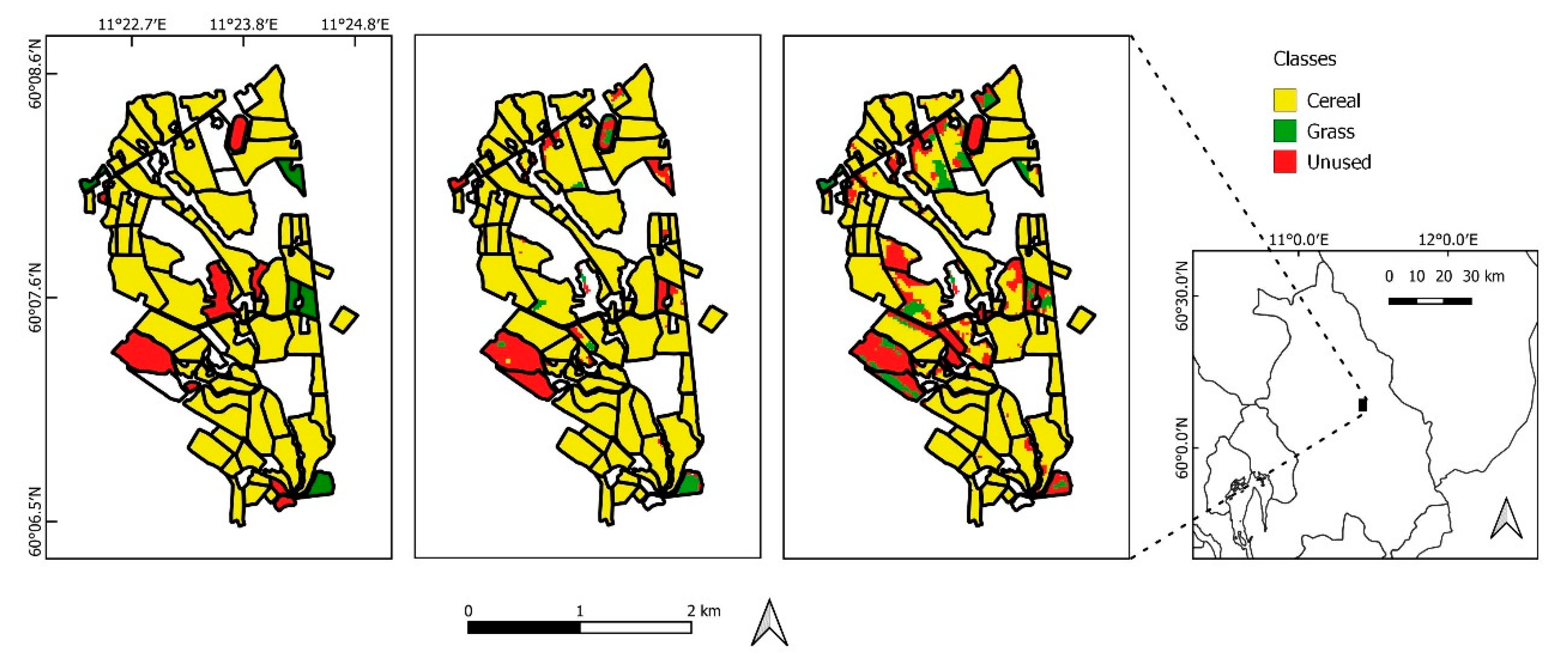
The predictive performances of the twelve different model–dataset combinations, as evaluated based on the JOVA and PT datasets, are presented in Table 4. The accuracy measures including precision, recall, F1 score for the three classes are presented. Although the 2D CNN on 7 days data performed best in training and on the test dataset, it is the 1D CNN implemented on the same dataset that performed best in the predicted dataset outside the training condition. Of the three seasonal land use classes, cereal was predicted most accurately in almost all the cases. The unused areas were predicted with the lowest accuracy in all cases, although they had similar accuracy during the training and the test datasets. For visual comparison, Figure 5 presents example field data from the JOVA dataset and a prediction by the 1D CNN and 2 D CNN using SITS data with a temporal resolution of 7 days.
4. Discussion
Four major results are presented in the above section: namely, temporal signatures of the three different seasonal land use classes, the architectures (hyperparameters) of the optimized models of the twelve model–dataset combinations, the accuracies of the model–dataset combinations as evaluated on held-out test data, and the predictive performances of the selected models. These results will be discussed here.
The spectral differences between the different land use classes are the basis for the use of remote sensing in land use classification. In this work, emphasis is given to the temporal signature, as the central theme of the work is time-series data. As shown in Figure 3, there is a difference in the temporal signature between cereals and the other two classes. Cereals have a distinct SAVI temporal signature that starts to increase from late spring and early summer, attaining its peak during the summer, and decreases again during the autumn. This is expected, as cereals are sown in spring and harvested in autumn. Between those times, the cereals continue changing their vigor, which manifests in the SAVI temporal signature. The SAVI temporal signature of grass, on the other hand, shows some deep drops. Such a decline in SAVI can be explained by the multiple harvests of grass during the growing season. In Norway, grass is harvested and stored for use as fodder during the winter. The frequency of the harvest depends on the growing season and the growing conditions. The unused areas, however, lack a distinct spectral or temporal signature, as they are formed of numerous surface types. The one shown in the figure as an example is close to that of grass, as most unused areas are left alone for natural growth. In most cases, on unused areas, grass establishes first, which is gradually overtaken by bushes and shrubs. They finally give way to forest regeneration if left to the natural succession process. The distinctness of a spectral–temporal signature, or lack thereof, directly affects the success of classification and mapping of the class using either traditional image classification or machine learning algorithms, including the deep learning algorithms used in this work.
The use of the Keras tuner to optimize the hyperparameters gave interesting results, as presented in Table 2. Firstly, one does not need to use very deep layers to obtain good results. The best-performing models have hidden layers ranging from 2 to 4. Deeper layers produce overfit models that do not generalize well and are computationally inefficient. Secondly, the activation function ReLU is selected in all cases, as is theoretically claimed [12]. Thirdly, the number and size of the filters in the CNN algorithms is, interestingly, related to the dimensions. A higher number of filters is found to be optimal for the 1D CNN, rather than for the 2D CNN. This is explained by the fact that the 2D CNN already involves a large number of features, as feature number increases exponentially with dimension. The optimum filter size is also larger for the 1D CNN. The spectral dimension is limited to 6. Therefore, filter sizes larger than 5 are not practical for the 2D CNN. In the case of the 1D CNN, the filters can be larger depending on the size of the temporal dimension. A larger filter along the temporal dimension can extract temporal features over a longer period. Therefore, a filter size of 7 is found to be optimum for the 1D CNN. It appears that the 1D CNN compensates for its lower dimension by increasing the size and number of filters. Fourthly, the optimum dropout rate is higher when the number of features increases, as in the case of 2D CNN. The dropout rate is lower for the 1D CNN and the MLP. A low rate of regularization is considered as optimum, indicating that, as other overfitting measures such as dropout and batch normalization are included, the need for regularization is not as great.
As presented in the results section, the 2D CNN performs best compared to the other models. The 2D CNN extracts a greater number of features than the 1D CNN, but it can also be susceptible to overfitting, as some of these features do not necessarily contribute much. This can explain the higher rate of dropout in the 2D CNN. Additionally, both the temporal and the spectral orders are considered when using 2D kernels. Differences in the spectral characteristics of different land cover classes form the basis of land use/cover mapping using remotely sensed data. Additionally, the seasonal variation in the different land use types is also important. For example, unused areas simply a follow natural growth succession, while cereal and grass fields are susceptible to human interference, which also has different specific time periods. The temporal dimension captures this temporal signature of the different land use classes. The use of both complements each other and increases the performance of the model. The 1D CNN disregards the spectral order; although it is included in the analysis, the orderly signature is not captured by the 1D kernel. Therefore, although its convolutional method outperforms the MLP, its disregard of the spectral order makes its performance lower than that of the 2D CNN. However, one interesting fact is that the 1DCNN performed better than the 2D CNN in terms of prediction, at least for the areas in which we had field data, when using the same temporal resolution. This can be attributed to better generalization by the former, owing to the larger filter, and more overfitting by the later.
Both the 1D and 2D CNN have increased the level of accuracies compared to the baseline algorithm, i.e., the MLP, applied on the same dataset, as can be observed in Figure 4. Even if the MLP is simple and can be used as a baseline, its hyperparameters need optimization to obtain the best performance. Considering the ease of application and efficiency of computation, the accuracies achieved by the MLP are appreciable and make it relevant in practical uses. Although systematic comparison of computational efficiencies is not part of this study, and hence not presented in the results, it is observed that the MLP is at least ten times faster than the 1D CNN, which in turn is about four times faster than the 2D CNN when similar depths are used. If one chooses to use the MLP for computational reasons, there will, consequently, be an accuracy trade-off.
The level of accuracies obtained, which ranges between 87% and 94%, is comparable to that of other studies of similar purpose. For example, [7] applied Random Forest (RF), ensembles of MLP and CNN (both 1D and 2D) to multitemporal and multisource images to classify crop types. Their overall accuracies varied from 88.7 (RF) to 94.6 % (2D CNN). Additionally, [25] applied 3D CNN on multitemporal images to classify crop types, and compared this with 2D CNN and other conventional methods. In agreement with our result, the CNN that involves the temporal dimension (3D CNN) produced the highest accuracy. Their technique uses 3D kernels, where pixels are not evaluated independently of adjacent pixels. Another relevant work is an early attempt at crop type classification by applying the RF classifier to mono-temporal Sentinel-2 images, which produced overall accuracies of 76% and 83% when object-based and pixel-based classification were used, respectively [41]. The overall accuracy improved considerably (reaching 95%) when multi-temporal images were used on the same area in a later study [42]. There is potential for improving the accuracy if the optical SITS data are supplemented with SAR SITS data, as demonstrated in a study by [43]. The studies mentioned, in agreement with the present study, highlight the importance of the temporal dimension in crop-type and land-use mapping using satellite images. The studies use different setups, data and methods to compare their quantitative performances to the results of the present work. Comparison to state-of-the-art benchmark algorithms was also not part of this work. State-of-the-art benchmark algorithms for time series classification are analyzed and compared in [19] and [44]. The approach presented here could be included in future analysis and comparison of state-of-the art algorithms for time series classification.
Regarding the temporal resolutions, the 7 days dataset produced the best accuracy. Obtaining cloud-free images within a 7 days interval is often difficult. Some of the data were obtained by interpolation. The interpolation does not seem to affect the expected high accuracy from the highest temporal resolution, i.e., 7 days. As the temporal resolution gets worse, so does the accuracy. More frequent temporal data capture the minor temporal differences between the different land use classes. Increasing the temporal gaps smoothens out such minor differences, making it harder to accurately classify the land use classes.
The most challenging part of this study was obtaining samples that represent the unused areas accurately. The unused areas are areas that are known to be agricultural fields but that are not used for crop production that qualifies for subsidies. By implication, the surface condition of the area varies considerably. This fact makes it difficult both to manually identify it and to detect it using remote sensing. The lack of uniqueness in its surface condition leads to a lack of uniqueness in its spectral–temporal properties as well. The unused areas represented in the training dataset are fitted well by the deep learning algorithms, as the test accuracy for the class “unused” was not much different from that of grass and cereal. However, when predicted for entirely unknown areas, the unused areas and grass were not well separated, leading to a higher precision but lower recall for grass. Some of the areas wrongly predicted as unused include grass, green houses in the middle of cereal fields and other crop types such as fruits.
5. Conclusions and Outlook
In this study, Sentinel-2 SITS data were used to map three agricultural land use classes by implementing deep learning algorithms. The study has demonstrated that by using time-series data from Sentinel-2, it is possible to discriminate between the major production classes, cereals, grasses, and areas out of production. The last class is the most heterogeneous. It was difficult to obtain a large and representative training dataset for this class, and thus the prediction for the class had a relatively low accuracy. We need to focus on this land use category and improve the accuracy before the procedure is implemented at a national level. One strategy is to split the heterogeneous unused land-use class into several classes and train a model that predicts more than three classes. The difficulty is in obtaining a sufficient amount of reliable data for this class.
The results have also indicated that SITS data of higher temporal resolution produce more accurate maps of land-use classes, as details of the spectral–temporal differences are learned, as opposed to SITS data of lower temporal resolution. Additionally, the results suggest that CNN is superior to MLP in learning such time series data. The 1D and 2D CNN perform similarly: one trains better while the other generalizes better. This similarity in performance might change if the SITS data have numerous spectral bands, for example, in the case of hyperspectral, as the 2D CNN can then use larger filter sizes. This is a question to be investigated in possible future works. Additionally, considering the ease of application and efficiency of computation, the accuracies achieved by the MLP are appreciable and make it relevant in practical uses.
The study has also demonstrated that temporal CNN, i.e., the use of temporal and spectral dimensions, is applicable and useful in Sentinel-2 images. The approach partially circumvents the limitations of using CNN in spatial dimensions on low-resolution satellite images. The results of the work are expected to be applicable to regions with similar topo-climatic conditions to Norway, i.e., similarities in the frequency of cloud coverage and topographic conditions.
Author Contributions
Conceptualization, M.D.-G. and A.K.G.; methodology, M.D.-G. and A.K.G.; analysis, M.D.-G. and A.K.G.; data curation, A.K.G.; writing—original draft preparation, M.D.-G.; writing—review and editing, A.K.G. and M.D.-G. All authors have read and agreed to the published version of the manuscript.
Funding
This research was funded partially by the Norwegian Space Agency, grant number NIT.05.19.5.
Institutional Review Board Statement
Not applicable.
Informed Consent Statement
Not applicable.
Acknowledgments
The authors are very grateful to Karsten Dax for helping prepare the training and validation data and Jonathan Rizzi for final proof reading of the manuscript.
Conflicts of Interest
The authors declare no conflict of interest.
References
- Agovino, M.; Casaccia, M.; Ciommi, M.; Ferrara, M.; Marchesano, K. Agriculture, climate change and sustainability: The case of EU-28. Ecol. Indic. 2019, 105, 525–543. [Google Scholar] [CrossRef]
- Howden, S.M.; Soussana, J.-F.; Tubiello, F.N.; Chhetri, N.; Dunlop, M.; Meinke, H. Adapting agriculture to climate change. Proc. Natl. Acad. Sci. USA 2007, 104, 19691–19696. [Google Scholar] [CrossRef] [Green Version]
- Ren, C.; Liu, S.; van Grinsven, H.; Reis, S.; Jin, S.; Liu, H.; Gu, B. The impact of farm size on agricultural sustainability. J. Clean. Prod. 2019, 220, 357–367. [Google Scholar] [CrossRef]
- Smith, C.; McDonald, G. Assessing the sustainability of agriculture at the planning stage. J. Environ. Manag. 1998, 52, 15–37. [Google Scholar]
- Wakker, W.; van der Molen, P.; Lemmen, C. Land registration and cadastre in the Netherlands, and the role of cadastral boundaries: The application of GPS technology in the survey of cadastral boundaries. J. Geospat. Eng. 2003, 5, 3–10. [Google Scholar]
- Pareeth, S.; Karimi, P.; Shafiei, M.; De Fraiture, C. Mapping agricultural landuse patterns from time series of Landsat 8 using random forest based hierarchial approach. Remote Sens. 2019, 11, 601. [Google Scholar] [CrossRef] [Green Version]
- Kussul, N.; Lavreniuk, M.; Skakun, S.; Shelestov, A. Deep learning classification of land cover and crop types using remote sensing data. IEEE Geosci. Remote Sens. Lett. 2017, 14, 778–782. [Google Scholar]
- Levitan, N.; Gross, B. Developing a Satellite-Based Remote Sensing System for Observing Maize Crop Growth. AGUFM 2018, 2018, GC51H-0885. [Google Scholar]
- Chlingaryan, A.; Sukkarieh, S.; Whelan, B. Machine learning approaches for crop yield prediction and nitrogen status estimation in precision agriculture: A review. Comput. Electron. Agric. 2018, 151, 61–69. [Google Scholar] [CrossRef]
- Mutanga, O.; Dube, T.; Galal, O. Remote sensing of crop health for food security in Africa: Potentials and constraints. Remote Sens. Appl. Soc. Environ. 2017, 8, 231–239. [Google Scholar]
- Gatti, A.; Bertolini, A. Sentinel-2 Products Specification Document. 2013. Available online: https://sentinel.esa.int/documents/247904/685211/Sentinel-2-Products-Specification-Document (accessed on 25 November 2020).
- Chollet, F. Deep Learning with Pyton; Manning Publications, Co.: Shelter Island, NY, USA, 2018. [Google Scholar]
- Panchal, G.; Ganatra, A.; Kosta, Y.; Panchal, D. Behaviour analysis of multilayer perceptrons with multiple hidden neurons and hidden layers. Int. J. Comput. Theory Eng. 2011, 3, 332–337. [Google Scholar] [CrossRef] [Green Version]
- Albawi, S.; Mohammed, T.A.; Al-Zawi, S. Understanding of a Convolutional Neural Network. In Proceedings of the 2017 International Conference on Engineering and Technology (ICET), Antalya, Turkey, 21–23 August 2017; pp. 1–6. [Google Scholar]
- Liang, M.; Hu, X. Recurrent Convolutional Neural Network for Object Recognition. In Proceedings of the IEEE Conference on Computer Vision and Pattern Recognition, Boston, MA, USA, 7–12 June 2015; pp. 3367–3375. [Google Scholar]
- Gardner, M.W.; Dorling, S.R. Artificial neural networks (the multilayer perceptron)—A review of applications in the atmospheric sciences. Atmos. Environ. 1998, 32, 2627–2636. [Google Scholar] [CrossRef]
- Guo, Y.; Liu, Y.; Oerlemans, A.; Lao, S.; Wu, S.; Lew, M.S. Deep learning for visual understanding: A review. Neurocomputing 2016, 187, 27–48. [Google Scholar] [CrossRef]
- Zhu, X.X.; Tuia, D.; Mou, L.; Xia, G.-S.; Zhang, L.; Xu, F.; Fraundorfer, F. Deep learning in remote sensing: A comprehensive review and list of resources. IEEE Geosci. Remote Sens. Mag. 2017, 5, 8–36. [Google Scholar] [CrossRef] [Green Version]
- Fawaz, H.I.; Forestier, G.; Weber, J.; Idoumghar, L.; Muller, P.-A. Deep learning for time series classification: A review. Data Min. Knowl. Discov. 2019, 33, 917–963. [Google Scholar] [CrossRef] [Green Version]
- Kussul, N.; Lavreniuk, M.; Shelestov, A.; Yailymov, B. Along the Season Crop Classification in Ukraine Based on Time Series of Optical and Sar Images Using Ensemble of Neural Network Classifiers. In Proceedings of the 2016 IEEE International Geoscience and Remote Sensing Symposium (IGARSS), Beijing, China, 10–15 July 2016; pp. 7145–7148. [Google Scholar]
- Zhang, Z.; Masjedi, A.; Zhao, J.; Crawford, M.M. Prediction of Sorghum Biomass Based on Image Based Features Derived from Time Series of UAV Images. In Proceedings of the 2017 IEEE International Geoscience and Remote Sensing Symposium (IGARSS), Fort Worth, TX, USA, 23–28 July 2017; pp. 6154–6157. [Google Scholar]
- Mou, L.; Ghamisi, P.; Zhu, X.X. Deep Recurrent Neural Networks for Hyperspectral Image Classification. IEEE Trans. Geosci. Remote Sens. 2017, 55, 3639–3655. [Google Scholar] [CrossRef] [Green Version]
- Wang, Z.; Yan, W.; Oates, T. Time Series Classification from Scratch with Deep Neural Networks: A Strong Baseline. In Proceedings of the 2017 International Joint Conference on Neural Networks (IJCNN), Anchorage, AK, USA, 14–19 May 2017; pp. 1578–1585. [Google Scholar]
- Kuang, D. A 1d convolutional network for leaf and time series classification. arXiv 2019, arXiv:1907.00069. [Google Scholar]
- Ji, S.; Zhang, C.; Xu, A.; Shi, Y.; Duan, Y. 3D convolutional neural networks for crop classification with multi-temporal remote sensing images. Remote Sens. 2018, 10, 75. [Google Scholar] [CrossRef] [Green Version]
- Pelletier, C.; Webb, G.I.; Petitjean, F. Temporal convolutional neural network for the classification of satellite image time series. Remote Sens. 2019, 11, 523. [Google Scholar] [CrossRef] [Green Version]
- Chen, K.; Wu, A.; Chern, J.; Chen, L.; Chang, W. FORMOSAT-2 Mission: Current Status and Contributions to Earth Observations. Proc. IEEE 2010, 98, 878–891. [Google Scholar] [CrossRef]
- Pan, Z.; Hu, Y.; Cao, B. Construction of smooth daily remote sensing time series data: A higher spatiotemporal resolution perspective. Open Geospat. Data Softw. Stand. 2017, 2, 25. [Google Scholar] [CrossRef] [Green Version]
- Buitinck, L.; Louppe, G.; Blondel, M.; Pedregosa, F.; Mueller, A.; Grisel, O.; Niculae, V.; Prettenhofer, P.; Gramfort, A.; Grobler, J. API design for machine learning software: Experiences from the scikit-learn project. arXiv 2013, arXiv:1309.0238. [Google Scholar]
- Abadi, M.; Barham, P.; Chen, J.; Chen, Z.; Davis, A.; Dean, J.; Devin, M.; Ghemawat, S.; Irving, G.; Isard, M. Tensorflow: A System for Large-Scale Machine Learning. In Proceedings of the 12th Symposium on Operating Systems Design and Implementation, Savannah, GA, USA, 2–4 November 2016; pp. 265–283. [Google Scholar]
- Gao, B.; Pavel, L. On the Properties of the Softmax Function with Application in Game Theory and Reinforcement Learning. arXiv 2017, arXiv:1704.00805. [Google Scholar]
- Ramchoun, H.; Idrissi, M.A.J.; Ghanou, Y.; Ettaouil, M. Multilayer Perceptron: Architecture Optimization and Training. IJIMAI 2016, 4, 26–30. [Google Scholar] [CrossRef]
- Alom, M.Z.; Taha, T.M.; Yakopcic, C.; Westberg, S.; Sidike, P.; Nasrin, M.S.; Hasan, M.; Van Essen, B.C.; Awwal, A.A.; Asari, V.K. A state-of-the-art survey on deep learning theory and architectures. Electronics 2019, 8, 292. [Google Scholar] [CrossRef] [Green Version]
- O’Malley, T.; Bursztein, E.; Long, J.; Chollet, F.; Jin, H.; Invernizzi, L. Keras Tuner. 2019. Available online: https://github.com/keras-team/keras-tuner (accessed on 11 December 2020).
- Krizhevsky, A.; Sutskever, I.; Hinton, G.E. Imagenet classification with deep convolutional neural networks. Commun. ACM 2017, 60, 84–90. [Google Scholar] [CrossRef]
- Ioffe, S.; Szegedy, C. Batch normalization: Accelerating deep network training by reducing internal covariate shift. arXiv 2015, arXiv:1502.03167. [Google Scholar]
- Neyshabur, B.; Bhojanapalli, S.; McAllester, D.; Srebro, N. Exploring Generalization in Deep Learning. In Proceedings of the Advances in Neural Information Processing Systems, Long Beach, CA, USA, 4–9 December 2017; pp. 5947–5956. [Google Scholar]
- Shorten, C.; Khoshgoftaar, T.M. A survey on Image Data Augmentation for Deep Learning. J. Big Data 2019, 6, 60. [Google Scholar] [CrossRef]
- Alvarez, S.A. An Exact Analytical Relation among Recall, Precision, and Classification Accuracy in Information Retrieval; Technical Report BCCS-02-01; Department of Computer Science, Boston College: Chestnut Hill, MA, USA, 2002. [Google Scholar]
- Qi, J.; Chehbouni, A.; Huete, A.R.; Kerr, Y.H.; Sorooshian, S. A modified soil adjusted vegetation index. Remote Sens. Environ. 1994, 48, 119–126. [Google Scholar] [CrossRef]
- Immitzer, M.; Vuolo, F.; Atzberger, C. First experience with Sentinel-2 data for crop and tree species classifications in central Europe. Remote Sens. 2016, 8, 166. [Google Scholar] [CrossRef]
- Vuolo, F.; Neuwirth, M.; Immitzer, M.; Atzberger, C.; Ng, W.-T. How much does multi-temporal Sentinel-2 data improve crop type classification? Int. J. Appl. Earth Obs. Geoinf. 2018, 72, 122–130. [Google Scholar] [CrossRef]
- Inglada, J.; Vincent, A.; Arias, M.; Marais-Sicre, C. Improved Early Crop Type Identification by Joint Use of High Temporal Resolution SAR and Optical Image Time Series. Remote Sens. 2016, 8, 362. [Google Scholar] [CrossRef] [Green Version]
- Bagnall, A.; Lines, J.; Bostrom, A.; Large, J.; Keogh, E. The great time series classification bake off: A review and experimental evaluation of recent algorithmic advances. Data Min. Knowl. Discov. 2017, 31, 606–660. [Google Scholar] [CrossRef] [Green Version]
Figure 1.
Spatial data model of the NetCDF data format (x = latitude, y = longitude, b = spectral bands (thematic layers) and t = time).
Figure 1.
Spatial data model of the NetCDF data format (x = latitude, y = longitude, b = spectral bands (thematic layers) and t = time).

Figure 2.
Schematic depiction of the 2D Convolutional Neural Network (CNN) model architecture used.

Figure 3.
The temporal signatures of the Soil Adjusted Vegetation Index (SAVI) of the three land use classes, i.e., cereal (top), grass (middle) and unused (lower), as obtained from their respective typical pixels (dashed lines) and sample pixels (scattered plots).
Figure 3.
The temporal signatures of the Soil Adjusted Vegetation Index (SAVI) of the three land use classes, i.e., cereal (top), grass (middle) and unused (lower), as obtained from their respective typical pixels (dashed lines) and sample pixels (scattered plots).

Figure 4.
Test of overall accuracies and Cohen’s Kapa of the twelve model–dataset combinations, as obtained based on the test datasets.
Figure 4.
Test of overall accuracies and Cohen’s Kapa of the twelve model–dataset combinations, as obtained based on the test datasets.

Figure 5.
Comparison of the land use types as registered in the Norwegian Agricultural Environmental Monitoring Program (JOVA)-dataset (left), with the prediction using the dataset with temporal resolution of 7 days and the 1DCNN model (middle) and the 2DCNN model(right).
Figure 5.
Comparison of the land use types as registered in the Norwegian Agricultural Environmental Monitoring Program (JOVA)-dataset (left), with the prediction using the dataset with temporal resolution of 7 days and the 1DCNN model (middle) and the 2DCNN model(right).


Table 1.
The parameter spaces used in Keras tuner for the deep learning models used in this work.
| No. | Parameter | Value Domain | Steps |
|---|---|---|---|
| 1 | Number of layers | [2, 7] | 1 |
| 2 | Number of neurons (units) | [32, 128] | 32 |
| 3 | Drop-out rate | [0.0, 0.5] | 0.05 |
| 4 | Activation function | [tanh, ReLU, SELU, SGM] | Choice |
| 5 | Learning rate | [1 × 10⁻⁵, 1 × 10⁻⁴, 1 × 10⁻³, 1 × 10⁻²] | Choice |
| 6 | Number of filters * | [32, 128] | 32 |
| 7 | Kernel size * | [3, 7] | 2 |
| 8 | Weight Regularization (L1L2) | [1 × 10⁻⁶, 1 × 10⁻⁵, 1 × 10⁻⁴, 1 × 10⁻³] | Choice |
* not applicable for the Multilayer Perceptron (MLP) model.
Table 2.
The hyperparameter values of the optimized models as obtained by using the randomized search method of Keras tuner.
Table 2.
The hyperparameter values of the optimized models as obtained by using the randomized search method of Keras tuner.
| Model | MLP | MLP | MLP | MLP | 1D CNN | 1D CNN | 1D CNN | 1D CNN | 2D CNN | 2D CNN | 2D CNN | 2D CNN |
|---|---|---|---|---|---|---|---|---|---|---|---|---|
| Temporal resolution | 7d | 14d | 21d | 28d | 7d | 14d | 21d | 28d | 7d | 14d | 21d | 28d |
| Input size | (N,162) | (N,84) | (N,54) | (N,42) | (N,6,27) | (N,6,14) | (N,6,9) | (N,6,7) | (N,6,27,1) | (N,6,14,1) | (N,6,9,1) | (N,6,7,1) |
| Number of hidden layers | 2 | 2 | 3 | 2 | 4 | 4 | 4 | 4 | 4 | 4 | 4 | 4 |
| No. of Units (neurons) | 128 | 128 | 96 | 96 | 96 | 96 | 96 | 96 | 128 | 128 | 128 | 128 |
| No. of filters | NA | NA | NA | NA | 128 | 128 | 128 | 128 | 64 | 64 | 64 | 64 |
| Drop-out rate | 0 | 0 | 0 | 0.05 | 0.15 | 0.15 | 0.15 | 0.15 | 0.25 | 0.25 | 0.25 | 0.25 |
| Activation | ReLU | ReLU | ReLU | ReLU | ReLU | ReLU | ReLU | ReLU | ReLU | ReLU | ReLU | ReLU |
| Learning rate | 1 × 10⁻³ | 1 × 10⁻³ | 1 × 10⁻³ | 1 × 10⁻³ | 1 × 10⁻⁴ | 1 × 10⁻⁴ | 1 × 10⁻⁴ | 1 × 10⁻⁴ | 1 × 10⁻³ | 1 × 10⁻³ | 1 × 10⁻³ | 1 × 10⁻³ |
| Kernel size | NA * | NA | NA | NA | 7 | 7 | 7 | 7 | 3 | 3 | 3 | 3 |
| Weight Regularization (L1L2) | 1 × 10⁻⁶ | 1 × 10⁻⁶ | 1 × 10⁻⁵ | 1 × 10⁻⁵ | 1 × 10⁻⁶ | 1 × 10⁻⁶ | 1 × 10⁻⁶ | 1 × 10⁻⁶ | 1 × 10⁻⁶ | 1 × 10⁻⁶ | 1 × 10⁻⁶ | 1 × 10⁻⁶ |
* Not Applicable.
Table 3.
Classification accuracies of the 2D CNN applied to the Sentinal-2 satellite image time series (SITS) data with 7 days temporal interval.
Table 3.
Classification accuracies of the 2D CNN applied to the Sentinal-2 satellite image time series (SITS) data with 7 days temporal interval.
| Class | Precision | Recall | f1-Score | Support |
|---|---|---|---|---|
| Cereal | 0.94 | 0.92 | 0.93 | 3266 |
| Grass | 0.95 | 0.92 | 0.93 | 3081 |
| Unused | 0.93 | 0.96 | 0.95 | 6273 |
| Overall accuracy | 0.94 | 12,620 | ||
| Macro average | 0.94 | 0.93 | 0.94 | 12,705 |
| Weighted average | 0.94 | 0.94 | 0.94 | 12,705 |
Table 4.
Prediction accuracies of the twelve optimized model–dataset combinations as evaluated using the JOVA and PT data.
Table 4.
Prediction accuracies of the twelve optimized model–dataset combinations as evaluated using the JOVA and PT data.
| Model-Dataset/Class | MLP_7d | MLP_14d | MLP_21d | MLP_28d | 1DCNN_7d | 1DCNN_14d | 1DCNN_21d | 1DCNN_28d | 2DCNN_7d | 2DCNN_14d | 2DCNN_21d | 2DCNN_28d |
|---|---|---|---|---|---|---|---|---|---|---|---|---|
| Cereal P | 1.00 | 1.00 | 1.00 | 1.00 | 1.00 | 1.00 | 1.00 | 1.00 | 1.00 | 1.00 | 1.00 | 1.00 |
| Cereal R | 0.96 | 0.94 | 0.89 | 0.87 | 0.98 | 0.98 | 0.84 | 0.90 | 0.93 | 0.93 | 0.89 | 0.95 |
| Cereal F1 | 0.98 | 0.97 | 0.94 | 0.93 | 0.99 | 0.99 | 0.91 | 0.95 | 0.96 | 0.96 | 0.94 | 0.97 |
| Cereal Support | 76,422 | 76,422 | 76,422 | 76,422 | 76,422 | 76,422 | 76,422 | 76,422 | 76,422 | 76,422 | 76,422 | 76,422 |
| Grass P | 0.81 | 0.83 | 0.84 | 0.84 | 0.82 | 0.82 | 0.83 | 0.85 | 0.80 | 0.84 | 0.84 | 0.84 |
| Grass R | 0.82 | 0.80 | 0.75 | 0.76 | 0.83 | 0.84 | 0.76 | 0.77 | 0.86 | 0.81 | 0.75 | 0.78 |
| Grass F1 | 0.82 | 0.82 | 0.79 | 0.80 | 0.82 | 0.83 | 0.79 | 0.81 | 0.83 | 0.83 | 0.79 | 0.81 |
| Grass Support | 25,852 | 25,852 | 25,852 | 25,852 | 25,852 | 25,852 | 25,852 | 25,850 | 25,852 | 25,852 | 25,852 | 25,851 |
| Unused P | 0.43 | 0.39 | 0.30 | 0.29 | 0.48 | 0.48 | 0.25 | 0.33 | 0.36 | 0.38 | 0.30 | 0.41 |
| Unused R | 0.52 | 0.60 | 0.65 | 0.65 | 0.55 | 0.53 | 0.61 | 0.67 | 0.50 | 0.61 | 0.65 | 0.64 |
| Unused F1 | 0.47 | 0.47 | 0.41 | 0.40 | 0.51 | 0.51 | 0.35 | 0.44 | 0.42 | 0.47 | 0.42 | 0.50 |
| Unused Support | 9923 | 9923 | 9923 | 9923 | 9923 | 9923 | 9923 | 9923 | 9923 | 9923 | 9923 | 9923 |
| Overall Accuracy | 0.89 | 0.88 | 0.83 | 0.82 | 0.91 | 0.91 | 0.80 | 0.85 | 0.87 | 0.88 | 0.83 | 0.88 |
Publisher’s Note: MDPI stays neutral with regard to jurisdictional claims in published maps and institutional affiliations. |
© 2021 by the authors. Licensee MDPI, Basel, Switzerland. This article is an open access article distributed under the terms and conditions of the Creative Commons Attribution (CC BY) license (http://creativecommons.org/licenses/by/4.0/).
Share and Cite
MDPI and ACS Style
Debella-Gilo, M.; Gjertsen, A.K. Mapping Seasonal Agricultural Land Use Types Using Deep Learning on Sentinel-2 Image Time Series. Remote Sens. 2021, 13, 289. https://0-doi-org.brum.beds.ac.uk/10.3390/rs13020289
AMA Style
Debella-Gilo M, Gjertsen AK. Mapping Seasonal Agricultural Land Use Types Using Deep Learning on Sentinel-2 Image Time Series. Remote Sensing. 2021; 13(2):289. https://0-doi-org.brum.beds.ac.uk/10.3390/rs13020289
Chicago/Turabian StyleDebella-Gilo, Misganu, and Arnt Kristian Gjertsen. 2021. "Mapping Seasonal Agricultural Land Use Types Using Deep Learning on Sentinel-2 Image Time Series" Remote Sensing 13, no. 2: 289. https://0-doi-org.brum.beds.ac.uk/10.3390/rs13020289
Note that from the first issue of 2016, this journal uses article numbers instead of page numbers. See further details here.