Aerial Imagery Feature Engineering Using Bidirectional Generative Adversarial Networks: A Case Study of the Pilica River Region, Poland

Abstract

Generative adversarial networks (GANs) are a type of neural network that are characterized by their unique construction and training process. Utilizing the concept of the latent space and exploiting the results of a duel between different GAN components opens up interesting opportunities for computer vision (CV) activities, such as image inpainting, style transfer, or even generative art. GANs have great potential to support aerial and satellite image interpretation activities. Carefully crafting a GAN and applying it to a high-quality dataset can result in nontrivial feature enrichment. In this study, we have designed and tested an unsupervised procedure capable of engineering new features by shifting real orthophotos into the GAN’s underlying latent space. Latent vectors are a low-dimensional representation of the orthophoto patches that hold information about the strength, occurrence, and interaction between spatial features discovered during the network training. Latent vectors were combined with geographical coordinates to bind them to their original location in the orthophoto. In consequence, it was possible to describe the whole research area as a set of latent vectors and perform further spatial analysis not on RGB images but on their lower-dimensional representation. To accomplish this goal, a modified version of the big bidirectional generative adversarial network (BigBiGAN) has been trained on a fine-tailored orthophoto imagery dataset covering the area of the Pilica River region in Poland. Trained models, precisely the generator and encoder, have been utilized during the processes of model quality assurance and feature engineering, respectively. Quality assurance was performed by measuring model reconstruction capabilities and by manually verifying artificial images produced by the generator. The feature engineering use case, on the other hand, has been presented in a real research scenario that involved splitting the orthophoto into a set of patches, encoding the patch set into the GAN latent space, grouping similar patches latent codes by utilizing hierarchical clustering, and producing a segmentation map of the orthophoto.

1. Introduction

There is no doubt that aerial imagery is a source of valuable information about geographical space. The rapid development of remote sensing technology supported by a significant improvement in access to remote sensing imagery [1] led to an increased interest in the potential use of the collected material among academia, government, and private sector representatives in areas such as urban planning, agriculture, transport, etc. Substantial quantities of image data have become available in recent years thanks to opening public access to images acquired by satellites such as Landsat 8 [2], Sentinel-2 A/B [3], and Pléiades [4]. Furthermore, due to the epidemiological situation in Poland, the government decided to open access to national orthophoto resources [5]. Access to high-quality and properly curated image repositories undoubtedly promotes the development of new ideas and contributes to the emergence of various methods and techniques for analyzing collected data.

The use of aerial and satellite images in the basic task of remote sensing that deals with land cover and land use classification is indisputable. At an early stage of remote sensing development, the possibility of distinguishing certain spatial units by interpreting the spectral, textural, and structural features of the image was indicated. Olędzki postulated extracting homogenous fragments of satellite images called photomorphic units. These units were similar in terms of structure and texture and originated from natural processes and man-made transformations of the environment [6,7]. Descriptive definitions of image features were soon replaced by mathematical formulas [8]. Further development has led to the introduction of object classification procedures, in which, in addition to the brightness parameters of the image pixels, their neighborhood and the shape and size of the distinguished objects were taken into account [9]. Object-oriented analysis is based on databases and fuzzy logic. Probably the most popular implementation of this paradigm in remote sensing applications is in the one originally developed in eCognition [10]. These techniques have been successfully applied to research on landscape structure and forestry [11]. Referring to division units used in physico-geographic regionalization [12,13], Corine Land Cover [14,15], or for the purposes of ecological research [16,17], an additional meaning and hierarchical structure [18,19] can be also given to units distinguished from the landscape. At the same time, it is important to properly take care of the appropriate adjustments of the scale of the study and data relevant for the analyzed problem, so as not to overlook important features of the area that may affect the reliability of the analysis, i.e., to mitigate the issues connected with spatial object scaling and the scale problem [20]. What is important is that the separation of landscape units cannot be based only on image data [21]. It is also necessary to take into account data on lithology, morphogenesis, terrain, geodiversity [22], water, and vegetation. The latter is interesting due to the fact that vegetation is represented in remote sensing imagery to the greatest extent both in terms of properties and structure. Therefore, it has great potential for being utilized in landscape quantification [23]. It should be mentioned that the process of identifying landscape units is also affected by human activity and created by the cultural landscape. Another major achievement in remote sensing image classification is the introduction of algorithms based on neural networks [24].

The influence of machine learning and deep learning on contemporary remote sensing techniques and their support in geographical space analysis is undeniable [25]. There are multiple fascinating applications of machine learning (ML) and deep learning (DL) in the remote sensing domain like land use classification [26], forest area semantic segmentation [27], species detection [28], recognition of patches of alpine vegetation [29,30], classification of urban areas [31], roads detection [32], etc.

What a significant part of these studies have in common is the focus on utilizing convolutional neural network (CNN) architectures capable of solving problems that can be brought down to traditional computer vision (CV) tasks like semantic segmentation, instance segmentation, or classification. This is directly associated with the underlying mechanism that enables the network to encode complex image features. CNN’s convolutional filters are gradually trained to gain the ability to detect the presence of specific patterns. Frequently, the training routine is performed in a supervised manner. The model is presented with target data and uses it to learn the solution. Supervised learning is capable of achieving extraordinary results but at the same time relies on access to manually labeled data. Another incredibly interesting approach is to train the neural network without any pre-existing labels to let it discover the patterns on its own. Although unsupervised learning algorithms like clustering are well-known among remote sensing researchers, utilizing convolutional neural networks is still to gain trust. The way of training a neural network can be even more intriguing when you exchange human supervision with machine supervision, and let multiple neural networks control their learning progress and work like adversaries.

Generative adversarial networks (GANs) are constructed from at least one discriminator and one generator network. The main goal of these two networks is to compete with each other in the form of a two-player minimax game [33]. The generator tries to deceive the discriminator by producing artificial samples, and the discriminator assesses whether it is dealing with real or generator-originating samples. The generator network is producing samples from a specified data distribution by transforming vectors of noise [34]. This technique was successfully applied in multiple remote sensing activities from upsampling satellite imagery [35], deblurring [36] to artificial sample generation [37]. GANs’ artificial data creation capabilities are not the only aspect that makes them interesting for remote sensing. When exploring the theory behind GANs, one should observe that, to perform its work, the generator retains all the information needed to produce a complex sample using only a much simpler representation called the latent code [33]. In terms of spatial analysis, this means that the network is able to produce a realistic image of an area using only a handful of configuration parameters as input. In the classic approach to GANs, this image recipe is reserved only for artificially generated samples. It was the introduction of bidirectional GANs and adversarial feature learning [38] that allowed to extract the latent code from ground truth (real) samples. The novelty of this approach when applied to aerial imagery is that it allows performing advanced spatial analysis using lower-dimensional representations of the orthophoto computed by a state-of-the-art neural network rather than utilizing raw image data. This method resembles algorithms like principal component analysis (PCA) but, instead of treating the image on the pixel level, it operates on the spatial features level and, therefore, offers a richer analysis context. The projection, a latent vector, serves as a lightweight representation of the image and holds information about the strength, occurrence, and interaction between spatial features discovered during the network training. This interesting capability opens up new possibilities for geographical space interpretation such as

• extracting features to fit in a variety of machine learning and spatial analysis algorithms like geographically weighted regression, support vector machines, etc.;
• minimizing resource consumption when processing large areas;
• discovering new features of analyzed areas by carefully exploring the network latent space.

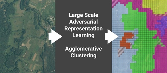
The principal goal of our study is to evaluate the potential of bidirectional generative adversarial networks in remote sensing feature engineering activities and unsupervised segmentation. Therefore, the following hypotheses have been defined:

• The image reconstruction process is strong enough to produce artificial images that closely resemble the original;
• Similar orthophoto patches can produce latent space codes that are close to each other in the network latent space, therefore, preserving the similarity after encoding;
• Latent codes enhanced by geographical coordinates can serve as artificial features used during geographical space interpretation by classical algorithms such as agglomerative clustering.

2. Materials and Methods

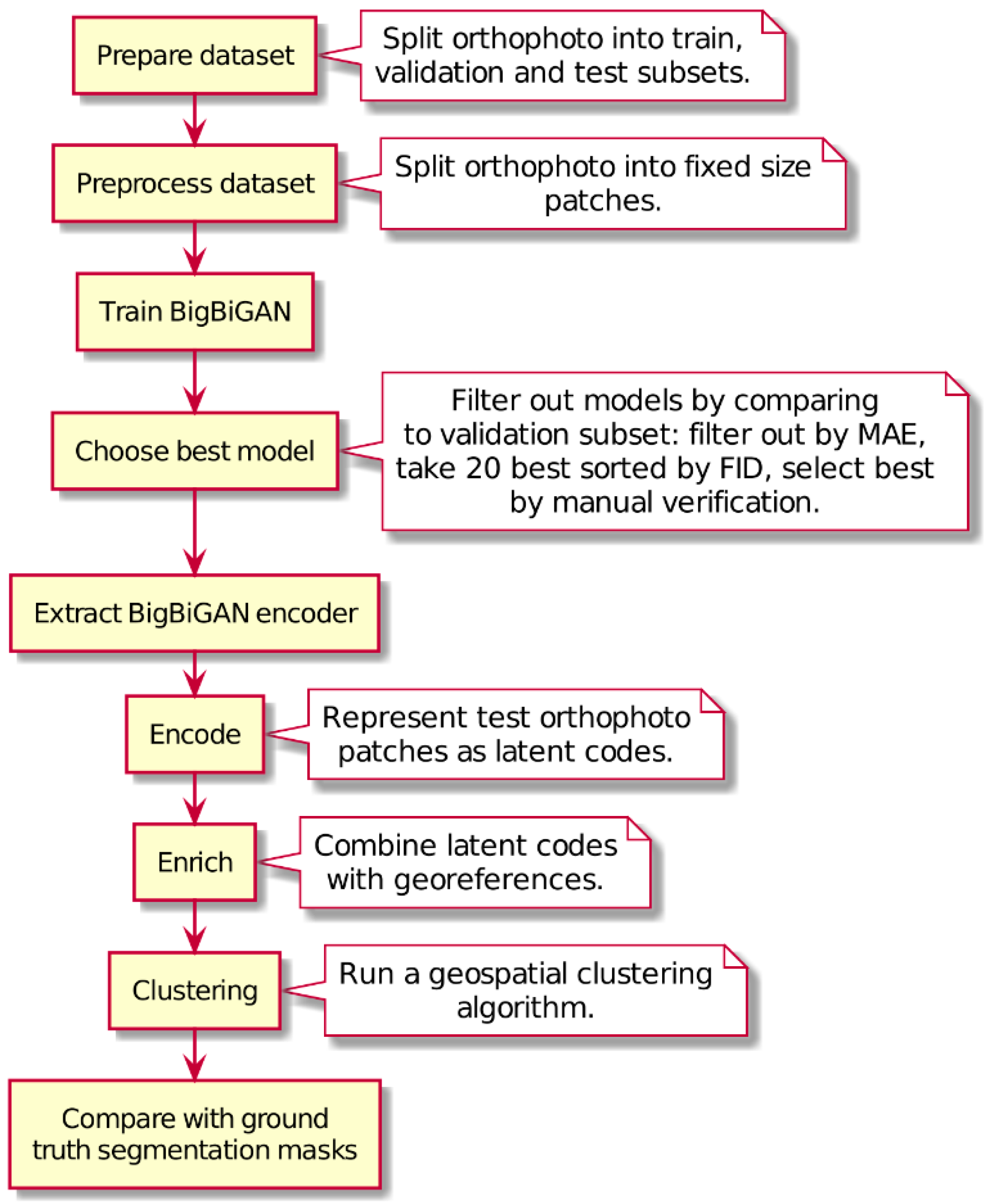
Figure 1 presents an overview of the proposed procedure composed of the following steps: preparing an orthophoto patches dataset, training the big bidirectional generative adversarial network (BigBiGAN), utilizing the network encoding module to convert orthophoto patches to their latent codes, enriching the data with geographical coordinates, and performing geospatial clustering on enriched latent codes.

2.1. Research Area

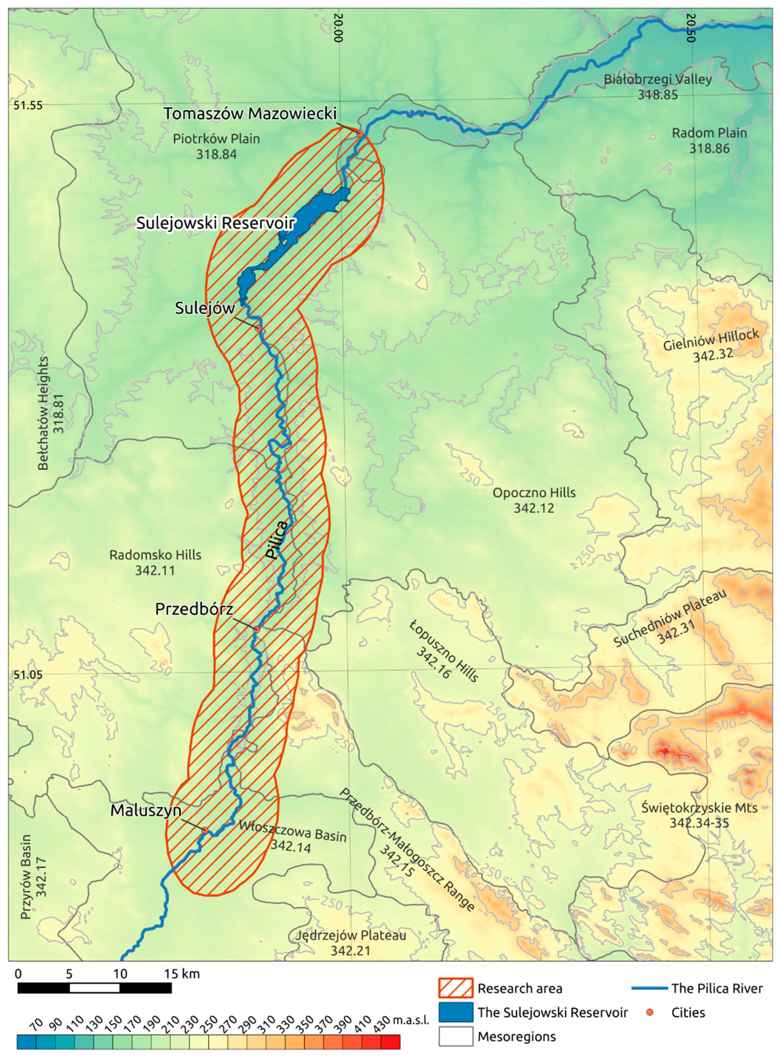
To be able to produce precise results, generative models need to be trained on high-quality datasets. The dataset needs to be large enough to cover the variety of spatial features that the encoder will be able to utilize when interpreting the input image. The authors decided to utilize RGB orthophotos of the Pilica River and Sulejowski Reservoir regions in Poland. The area from which the samples have been obtained includes the Plica River valley between Maluszyn and Tomaszów Mazowiecki together with adjacent areas (see Figure 2).

According to the physico-geographical regionalization of Poland [13], the southern and eastern parts of the area are located in the province of Polish Uplands, the macroregion of the Przedbórz Upland, the mesoregions of Włoszczowa Basin, Radomsko Hills, Przedbórz-Małogoszcz Range, and Opoczno Hills. The northwestern part is located in the mesoregions of the Piotrków Plain and the Białobrzegi Valley, which are part of the South Mazovian Hills macroregion in the Central European Lowland Province. The consequence of the location in the border zone of the Polish Uplands and the Central European Lowland is the interpenetration of features characteristic of both provinces and the relative diversification of the natural environment of the area.

According to the tectonic regionalization [39], a fragment of the area located south of Przedbórz includes the Szczecin–Miechów Synclinorium, constructed mainly from Cretaceous rock formations. The rest of the area belongs to the Mid-Polish Anticlinorium, dominated by Jurassic carbonate rocks.

The axis of the selected area is the Pilica River valley. The chosen section of the valley is in a natural condition. The Pilica River flows in an unregulated, sinuous to a meandering channel that is not embanked along its entire length from Maluszyn to the vicinity of Sulejów. There, it reaches the Smardzewice dam waters of the Sulejowski Reservoir. The valley floor descends from 211 m above sea level in the south to 154 m above sea level in the north, and the stream gradient equals 0.51%. The width of the valley varies from about 300 m in the vicinity of Sulejów and Przedbórz to over 3 km near Łęg Ręczyński. It reaches its greatest width in places of well-formed levels of over-flood terraces occurring on both sides of the floodplain.

The valley cuts down the adjacent plain and undulating moraine uplands to about 20–25 m. These landforms were formed in the Quaternary, mainly during the Pleistocene glaciations of the Middle Polish Complex. Within the uplands on both sides of the Pilica River, the thickness of Quaternary sediments decreases from the north to the south. The surface area of Mesozoic outcrops increases, which is a result of the weakening of the landforming capacity of the ice sheets as they entered the uplands. Absolute heights of culminations, in the form of isolated hills built of Mesozoic Jurassic and Cretaceous rocks within the Radomsko and Opoczno Hills, are also increasing, e.g., Diabla Góra 272 m, Czartoria Range 267 m, Bąkowa Góra 282 m, the form of ridges in the Przedbórz–Małogoszcz Range exceeding 300 m above sea level, or Bukowa Góra 336 m.

The varied topography and the near-surface geological structures, in addition to the humidity conditions, shape the mosaic of land cover types. The area is poorly urbanized. The ground moraine plateaus are dominated by arable land, fluvioglacial plains, and other sandy areas largely occupied by forests and abandoned arable lands. In the valley, the over-flood terraces are characterized by complex systems of arable land, fallow land, forests, and meadows. The floodplain is dominated by meadows and pastures, in many places overgrown with shrubs and trees after their agricultural use ceased [41].

2.2. Dataset

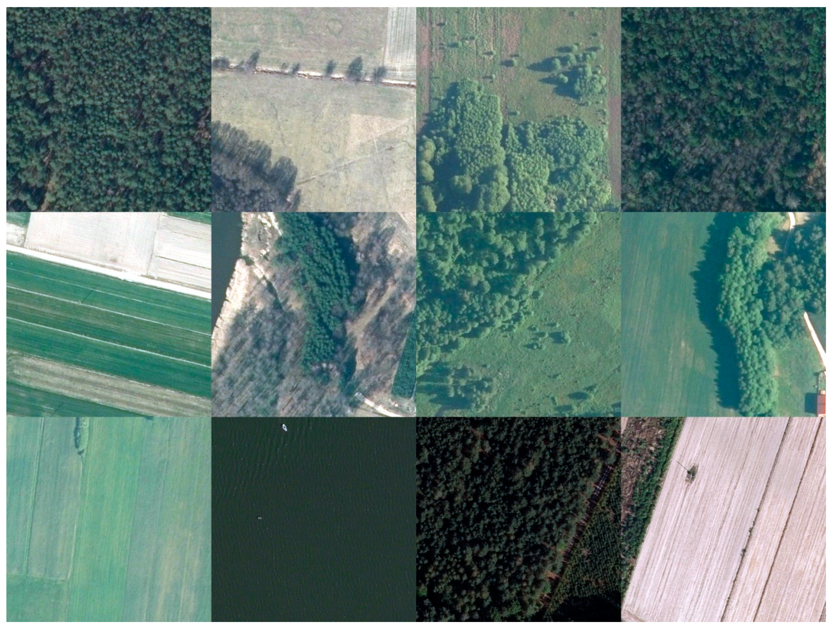
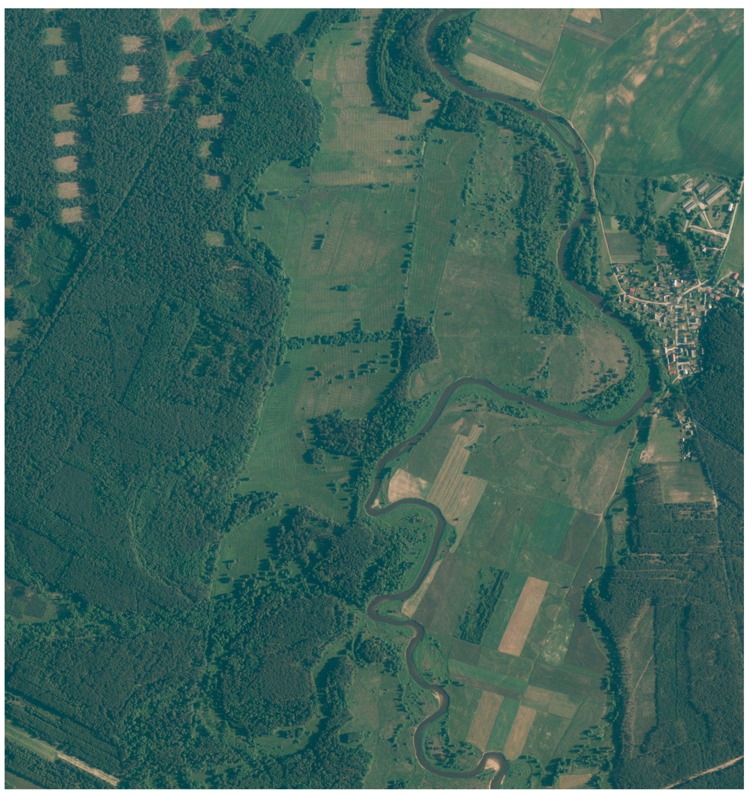
The Pilica River region dataset covers the area of 691.86 km² and was generated using 138 orthophoto sheets that intersect with a 4 km buffer around the Pilica River from Sulejów to Maluszyn and Sulejowski Reservoir in Łódź Voivodeship in Poland. All orthophotos were acquired using GEOPORTAL2 [42] and possess three channels—R-red, G-green, and B-blue with 25 cm pixel ground sample distance (see Figure 3).

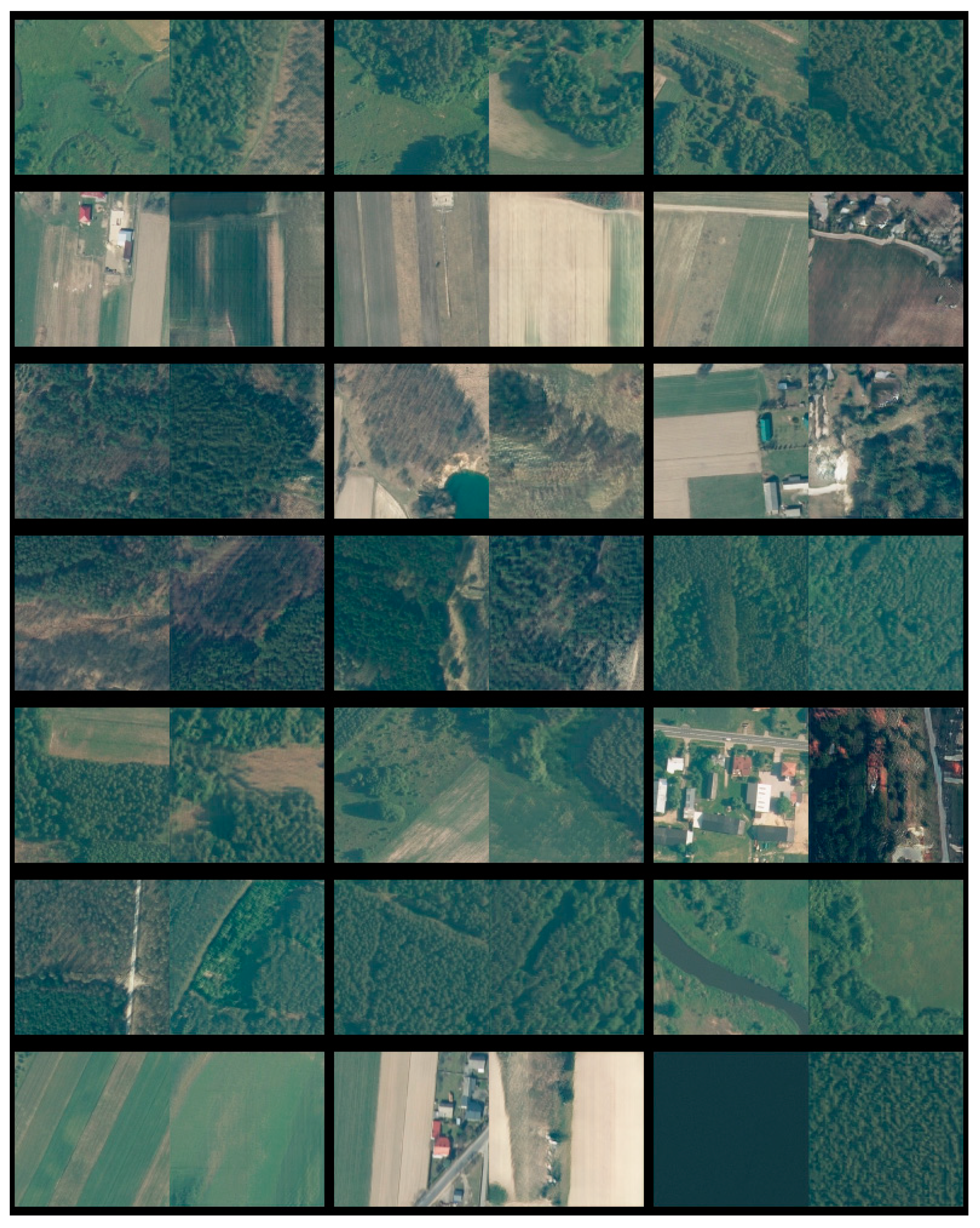
During the preprocessing phase each image was split into 128 px × 128 px, 256 px × 256 px, 512 px × 512 px, and 1024 px × 1024 px patches. This step was crucial for electing the optimal image size and resizing approach to satisfy the requirements of the chosen neural network architecture and its internal complexity. The choice of image size directly influences hardware requirements, the ability of the neural network to learn image features needed during the assessment of the reconstruction process, and, important from a GAN perspective, overall dataset size. It was highly important to utilize the patches large enough to be described by complete and interpretable spatial features. Image size also affects the size of the input and output tensors and the handful of technical parameters that a processing unit can handle. The authors decided that, during the research, a single GPU (Nvidia Titan RTX in US) and CPU (AMD Threadripper 1950 in US) will be used, and all computations have to fit their representative capacity. This is due to ensuring that the results can be reproduced without using a multi-GPU cluster. In consequence, the authors decided to utilize:

• A series of 256 px × 256 px patches for encoder input, which were resized from 512 px × 512 px patches using bilinear interpolation. Although 256 px × 256 px is either the network nor hardware limit, it gives the opportunity to choose a larger batch, which significantly affects BigBiGAN performance. Furthermore, 512 px × 512 px (128 m × 128 m) patch is richer in spatial information;
• A series of 128 px × 128 px patches for image discriminator input, explicitly defined by BigBiGAN architecture for 256 px × 256 px encoder input;
• A series of 128 px × 128 px patches for generator output, which were the minimal interpretable patch size.

Geographical references of each patch and source image metadata have been preserved to enable reprojecting the results back to their original location. Patches acquired from 137 images were divided, in accordance with the established practice of machine learning, into two subsets of 512 px × 512 px images in the following proportions 0.95 and 0.05, forming a training set (39826 patches) and validation set (2096 patches). Remaining images were also processed and formed two test sets—one containing 1224 (256 px × 256 px) patches and another containing 306 (512 px × 512 px) patches. The authors introduced an additional test set of 256 px × 256 px patches that were smaller than the defined training size to verify whether the solution is capable of handling input material potentially containing less spatial information than it was trained on.

Afterward, a data augmentation procedure was defined to increase the diversity of managed datasets by applying specified image transformations in a random manner. Augmentation of the dataset is important from the point of view of GAN because the network has a higher chance to adapt to different conditions such as lighting or spatial feature shape changes, and at the same time, less data is needed for the network to converge. The authors decided to utilize basic post-processing computer vision techniques, such as adding or subtracting a random value to all pixels in an image, blurring the image using gaussian kernels, applying random four-point perspective transformations, rotating with clipping, or flipping the image. What is important, each transformation was applied only during the training phase and the decision of whether to apply it was random. Finally, a TensorFlow data processing pipeline(US; Mountain View; California) was implemented to ensure that reading and augmenting the data would efficiently utilize all computational resources. The main goal was to support the GPU with constant data flow orchestrated by the CPU and enable shuffling across batches, which turned out to be crucial when working with complex network architectures and utilizing a relatively small batch size, i.e., below 128 samples.

2.3. Generative Adversarial Network

The authors decided to use the bidirectional generative neural network (BiGAN) [38] architecture as a starting point and gradually updated its elements to end up with the final solution closely resembling BigBiGAN. An interesting, proven property of these architectures is the ability to perform the inverse mapping from input data to the latent representation. This makes BiGAN and BigBiGAN great candidates to address the research problem, i.e., finding a transformation capable of mapping a multichannel image to a fixed size vector representation. BigBiGAN can be used to shift a real image to the latent space using the encoder network.

The resulting latent space code can be then utilized as generator input to reconstruct an image similar to the original encoder input. Achieving the same input and output is hard or even impossible due to the fact that the pixel-wise reconstruction quality is not even a task for bidirectional GANs, and therefore, there is no loss function assigned to assess it. One can think of reconstruction as a process of enabling a mechanism of lossy image compression and decompression that operates—not on pixel level—but feature level. The similarity measure can be chosen arbitrarily but has to have sufficient power to reliably score the resemblance of the input and output images passed through the encoder and generator. A high-quality encoder is powerful enough to store information regarding crucial spatial features of the input image, thus making it a great candidate for the main module in an automatic feature engineering mechanism to automatically generate large numbers of candidate properties and selecting the best by their information gain [43].

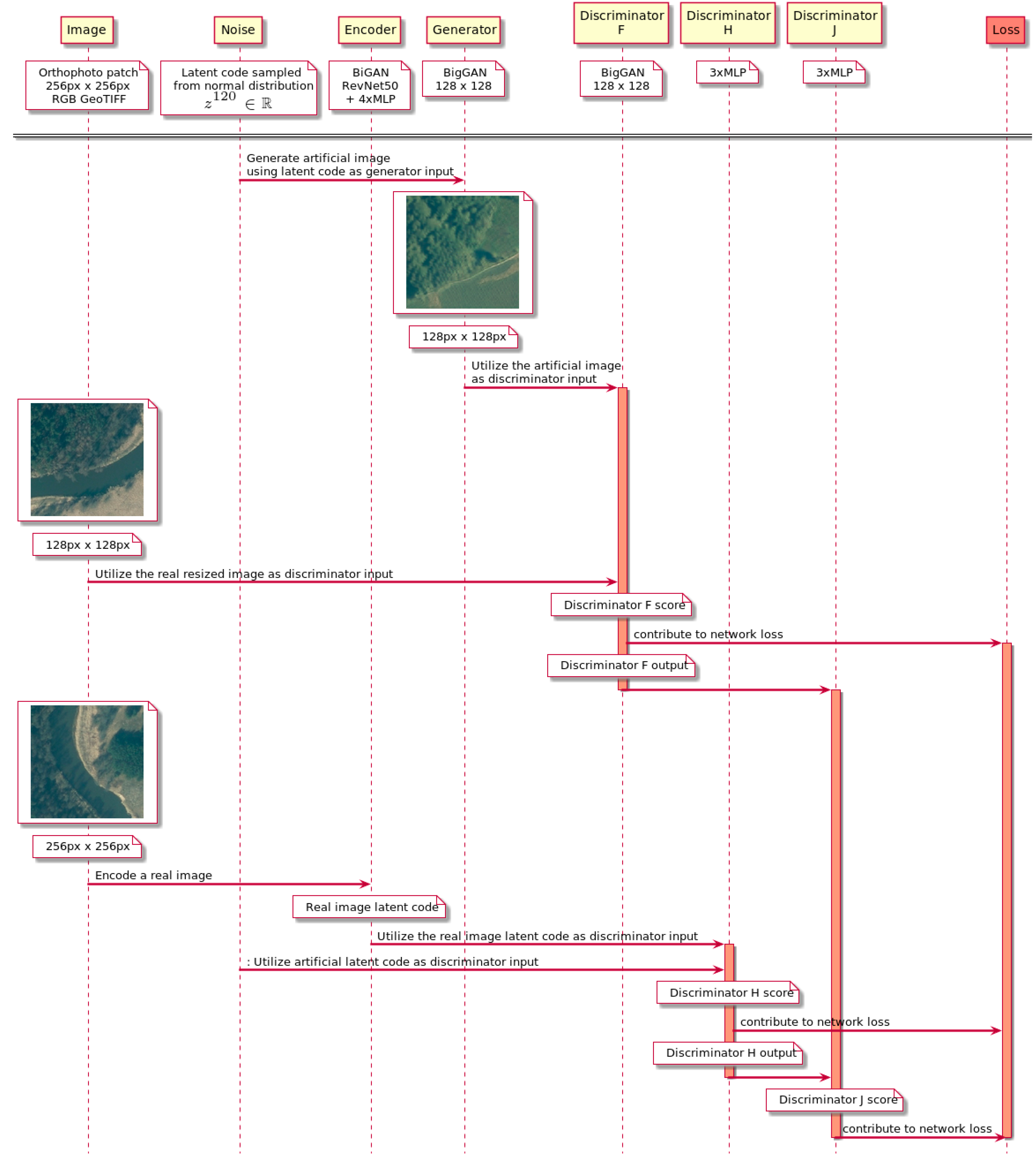
To avoid recreating an existing solution, the authors decided to focus on reusing the BigBiGAN design and adjusting it to processing orthophoto images (see Figure 4). BigBiGAN consists of five neural networks—a generator and an encoder, which are accompanied by discriminators that assess their performance in producing respectively artificial images and latent codes. Results from both intermediate discriminators are then combined by the main discriminator. In the research, a modification of BigBiGAN was utilized to tackle the problem of encoding orthophoto patches to the network underlying latent space. Although the generator and main discriminator architectures have been preserved, the encoder and intermediate discriminators went through a minor modification. As suggested in a study on the BigBiGAN [44], the RevNet model was simplified to reduce the number of parameters needed to train the encoder. Intermediate discriminators contained fewer multilayer perceptron modules (MLP), which were composed of smaller numbers of neurons. In consequence, this enabled the use of slightly bigger batches and, therefore, yielded better results at the cost of a training time increase. The final architecture was implemented in TensorFlow 2 and Keras. Figure 4 presents the final model training sequence blueprint.

2.4. Hierarchical Clustering

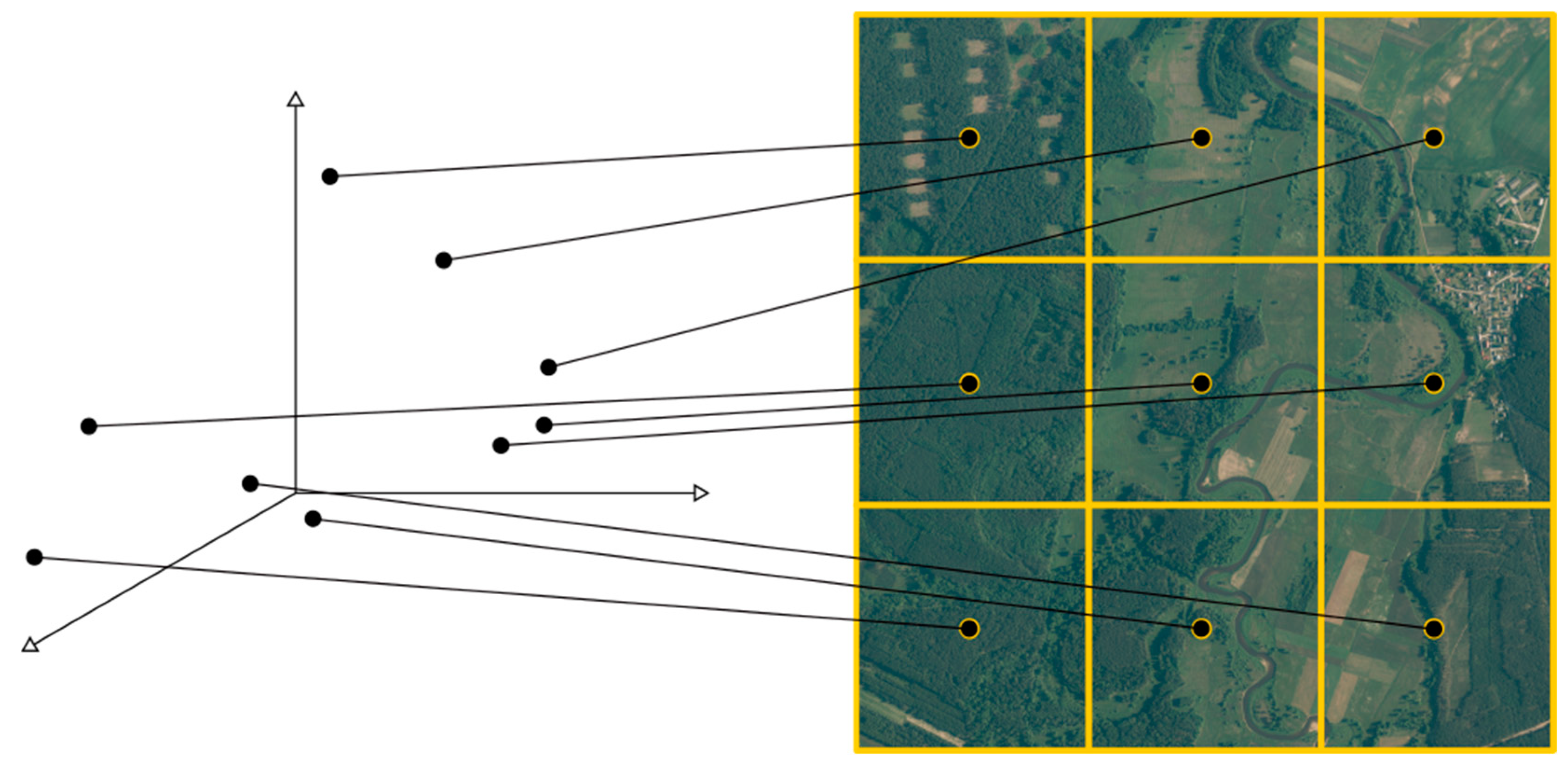
Latent space code is a 120-dimensional vector of real numbers produced by applying a GAN encoder on an orthophoto patch. Such code contains information regarding spatial features present in the scope of the encoded patch. Each part of the code controls the strength and occurrence of one or more spatial features discovered during the neural network training. One of the important features of the latent space is that codes that are closer to each other in terms of the Euclidean distance (L2 norm) are more similar in terms of the represented features, i.e., two forest area patches will be closer in the latent space than a forest area and farmland patches [45].

Furthermore, each patch holds information regarding its georeferences. To simplify further analyses, georeferences were expressed as the location of the patch center. Patch center geographical coordinates were preserved during the computation and combined with corresponding latent codes. This opened the possibility to describe a larger area, composed of multiple patches, in the form of a 120-dimensional point cloud where each point holds the information regarding its original location. The combination of georeferences and latent space code is called a georeferenced latent space for the purpose of this research (see Figure 5).

The similarity between patches, precisely between their encodings, and information regarding geographical location can serve as input for methods and techniques of geospatial clustering. During their research, the authors focused on utilizing hierarchical clustering to discover a predefined number of clusters in a patch dataset describing a single test orthophoto. Hierarchical clustering is a general family of clustering algorithms that build nested clusters by successively merging or splitting them [46]. The metric used for the merge strategy is determined by the linkage strategy. For the purpose of clustering the georeferenced latent space, Ward’s linkage method [47] was used. Ward’s method minimizes the sum of squared differences within all clusters. It is a variance-minimizing approach and, in this sense, is similar to the k-means objective function but tackled with an agglomerative hierarchical approach. The connectivity matrix has been calculated using the k-nearest neighbors algorithm (k-NN).

3. Results

3.1. Model Training

Multiple model training session revealed that tackling the objective of training an orthophoto patch encoder is inseparably related to preparing generator and discriminator neural networks that are complex enough to learn all the features present in the input orthophoto. The networks have to be able to produce high-quality artificial images and determine whether the image is artificially generated or not, respectively. This directly influences the following:

• The overall size of the neural network, which is crucial due to GPU memory limitations and affects training duration;
• Maximum patch size that can be used as input during training and inference phases and is related to the level of detail offered in the processed dataset;
• Batch size, which has a significant influence on the stability and quality of generative adversarial models [44].

Initially chosen BiGAN architecture utilizes many concepts from previously designed networks such as deep convolutional GAN (DCGAN) [48] that, due to their simplicity, are not suitable for processing complex or large images. Therefore, their usefulness in the analysis of aerial imagery is limited. Although BiGAN offered all of the required earlier features, it was not capable of processing an orthophoto patch of size exceeding 32 pixels in both dimensions. This was a huge limitation due to the fact that, with a given 25 cm pixel ground sample distance, this method covered roughly the area of 64 m². In consequence, the processed patch did not carry enough details to allow a reliable assessment of the similarity between real and artificial images. Attempts to increase the maximum processed input size led to swapping default BiGAN generator and discriminator models with other network types based on deep residual blocks [49] and inception modules [50]. The overall architecture of the generator and discriminator pair resembled BigGAN [51].

After multiple experiments, the authors confirmed that, despite the ability to generate images up to 512 px × 512 px, the network was not capable of learning a reliable bidirectional mapping between the image and the latent space. This was due to the fact that the encoder architecture was lacking in comparison with its powerful counterparts. This problem has been addressed and mitigated in the paper describing large adversarial features learning and the big bidirectional generative adversarial network (BigBiGAN) [44] by introducing intermediate discriminators and proposing a stronger encoder model (Supplementary Materials).

3.2. Reconstruction

BigBiGAN neural network was trained for 200,000 steps with a batch containing 32 randomly picked patches from the training set. The trained model was saved during each reconstruction period that occurred every 1000 steps. During this period, patches from the validation set were fed, in inference time, to the encoder and generator to measure their power in creating artificial samples and close to the inversible encoding in terms of spatial features. Three types of metrics were calculated for each saved model to evaluate the reconstruction quality—pixel-wise mean absolute error (MAE) of image values normalized between –1 and 1, Fréchet inception distance (FID) [52] on a pre-trained InceptionV3 model, and by performing perceptual evaluation similar to that presented in the Human Eye Perceptual Evaluation (HYPE) paper [53]. MAE above 0.5 was used to discard low-quality models that were not able to effectively reconstruct input images in the early stages of the training. Then, FID values of all preserved models were compared and 20 with the highest score were selected. The average FID score was equal to 86.36 ± 7.28 in contrast to the state-of-the-art BigBiGAN baseline FID, which was equal to 31.19 ± 0.37.

The final model was selected by comparing the results of human evaluation of 21 arbitrarily chosen samples from the validation dataset with their reconstructed counterparts created by the network for each model. The human reader had an objective to assess whether each of the 42 images is real or artificial. The last verification phase resulted in selecting the model from the 170th reconstruction period, which yielded the least accuracy during human perceptual evaluation (accuracy: 59.5%, f-score: 0.6663). Samples and their reconstruction results are presented in Figure 6.

The overall quality of the reconstruction was assessed as sufficient during both quantitative and qualitative verification. For the selected model evaluated on non-scaled images (pixel values between 0 and 255), MAE was 27.213, structural similarity index (SSIM) [54] was 0.942, and peak signal-to-noise ratio (PSNR) [55] was equal to 42.731. From the analysis of human reader’ misclassifications, it was clear that the chosen model is exceptionally good in reproducing areas like forests, land abandonment, and farmlands. The characteristic spatial features are preserved after encoding. Shadows cast by trees are consistent and natural. In the majority of cases, artificial and real images are indistinguishable. Mediocre results were achieved for urbanized areas. Reconstructed roads keep their linear character and surface type information. Although the model is capable of generating buildings, due to the high variety of housing types present in the research area and possible undersampling, the results are far from realistic. It is interesting that the link between residential areas and roads was maintained in multiple samples. Unfortunately, the generator is not capable of serving samples that contain water areas such as rivers or lakes. From all analyzed images from the training and validation set only a few presented water, which indicates weak encoding capabilities. Furthermore, all were significantly disrupted. The authors confirmed that this is related to undersampling and the insufficient information present in the RGB orthophoto. To tackle this issue, access to rich, multispectral imagery or digital terrain model (DTM) is required, or the model itself needs to be enriched to utilize additional class embeddings that could be derived from existing thematic maps or projects like Geoportal TBD [56].

3.3. Feature Engineering

BigBiGAN encoder possesses an interesting capability that enables it to shift the input image into the latent space constructed during network training. The encoding, a 120-dimensional vector, should be considered simultaneously a compressed version of the input orthophoto and a recipe for generating a similar artificial image in terms of spatial features. The latter phenomenon is called representation learning. What is important, due to the nature of latent space, similar data points, i.e., those that were encoded from similar images, are closer to each other. This opens an interesting possibility to understand the structural similarity between images by performing the analysis not on the raw image input but only using latent codes.

In the research, the authors utilized the trained encoder to perform inference on a set of 256 px × 256 px test patches (see Figure 7). The 1224 test patches were converted into their latent space codes and represented as a geopandas [57] data frame containing 1224 rows, 120 encoding value columns, identifier, and a geometry column. Afterward, distance weights between patch centroids were calculated utilizing the k-NN algorithm [58]. The data frame and distance weights served as input parameters to the agglomerative clustering algorithm. Figure 8 represents the results for a specified number of clusters.

Simultaneously, ground truth segmentation masks were prepared by manually dividing the test image into a fixed number of regions. For the number of clusters between 2 and 10, there was an average of 17.97% ± 8.7% patch-wise difference between ground truth and the unsupervised approach results. The more clusters were predicted the difference was larger. Figure 9 represents the best result, which was acquired for six clusters where the unsupervised approach misclassified 6% of patches.

4. Discussion

Utilizing a neural network as a key element of a feature engineering pipeline is a promising idea. The concept of learning the internal representation of data is not new and was extensively studied after the introduction of autoencoders (AE) [59]. Unlike regular autoencoders, bidirectional GANs do not make assumptions about the structure or distribution of the data making them agnostic to the domain of the data [38]. This makes them perfectly suited for use beyond working with RGB images and opens the opportunity to apply them in remote sensing where processing hyperspectral imagery is a standard use case.

One of the main challenges when utilizing a GAN is determining how big a research dataset is needed to feed the network to obtain the required result. The performance of the generator and, therefore, the overall quality of the reconstruction process and network encoding capabilities are tightly coupled with the input data. To be able to properly encode an image, BigBiGAN needs to learn different types of spatial features and discover how they interact with each other. In the early stages of the research, we identified that the size of the dataset had a positive influence on reconstruction quality. We initially worked with around 10% of the final dataset in order to rapidly prototype the solution. The results were not satisfying, i.e., we were not able to produce artificial samples that resembled ground truth data. This prompted us to gradually increase the dataset’s size. Authors are far from estimating the correct size of the dataset that could yield the best possible result for a specific research area. We are sure that addressing this issue will be important in the future development of this method.

The method of measuring the training progression of generative models still remains a problematic issue. The standard approach of monitoring the loss value during training and validation is not applicable due to the fact that all GAN components interact with each other, and the loss value is calculated against a specific point in time during the training process and, therefore, is ephemeral and incomparable with previous epochs. There are multiple ways of controlling how the training should progress, e.g., by using Wasserstein loss [60], applying gradient penalty [61], or spectral normalization [62]. Nevertheless, it is difficult to make a clear statement of what loss value identifies a perfectly trained network. Furthermore, applying GAN to tackle the problems within the remote sensing domain is still a novelty. It is difficult to find references in the scientific literature or open-source projects that could be helpful in determining the proper course of model training.

Although nontrivial, measuring the quality of bidirectional GAN image reconstruction capabilities seems to be a valid approach to the task of model quality assurance. An encoder, by design, always yields a result. It is just as true for a state-of-the-art model and its poorly trained counterparts. Encoder output cannot be directly interpreted, which makes it hard to evaluate its quality. The generator, on the other hand, produces a visible result that can be measured. According to the assumptions of bidirectional models, the encoding and decoding process should to some extent be reversible [38]. Hence, the artificially produced image should resemble, in terms of features, its reconstruction origin, i.e., the real image in which latent code was used to create an artificial sample. In other words, checking generator results operating on strictly defined latent codes determines the quality of the entire GAN.

A naive method of verification of the degree to which an orthophoto generated image looks realistic would be to directly compare it to its reconstruction origin. Pixel-wise mean absolute error (MAE) or a similar metric can give the researchers insight, to a limited extent, regarding the quality of produced samples. Unfortunately, this technique only allows getting rid of obvious errors such as a significant mistake in the overall color of the land cover. This is due to MAE not promoting textural and structural correctness, which may lead to poor diagnostic quality in some conditions [63]. One can approach a similar problem when using PNSR. To some extent, SSIM addresses the issue of measuring absolute errors by analyzing structural information. On the other hand, this method is not taking into account the location of spatial features. BigBiGAN reconstruction process only preserves features and their interaction not their specific placement in the analyzed image. Inception score (IS) and Fréchet inception distance (FID) address this problem by measuring the quality of the artificial sample by scoring the GAN capability to produce realistic features [34]. The main drawback of the IS is that it can be misinterpreted in case of mode collapse [64], i.e., the generator is able to produce only a single sample despite the latent code used as input. FID is much stronger in terms of assessing the quality of the generator. What is important, both metrics utilize a pre-trained Inception classifier [50] to capture relevant image features and therefore are dependent on its quality. There are multiple pre-trained models of Inception available. Many of them were created using large datasets such as ImageNet [65]. The authors are not aware of whether a similar dataset for aerial imagery exists. The use of FID is advisable and, as confirmed during the research, it is valuable in proving the capabilities of the generator, but it needs an Inception network trained on a dedicated aerial imagery dataset to be reliable. This way, the score calculated would depend on real spatial features existing in the geographical space. What is more, this approach is only applicable to RGB images. To perform FID calculation for hyperspectral images, a fine-tailored classifier should be trained. Not surprisingly, one of the most effective ways of verifying the quality of artificial images is through human judgment. This takes on even greater importance when approaching the research subject requires specialized knowledge and skills, as exemplified by the analysis of aerial or satellite imagery. Unfortunately, qualitative verification is time-consuming and has to be supported by a quantitative method, which can aid in preselecting potentially good samples.

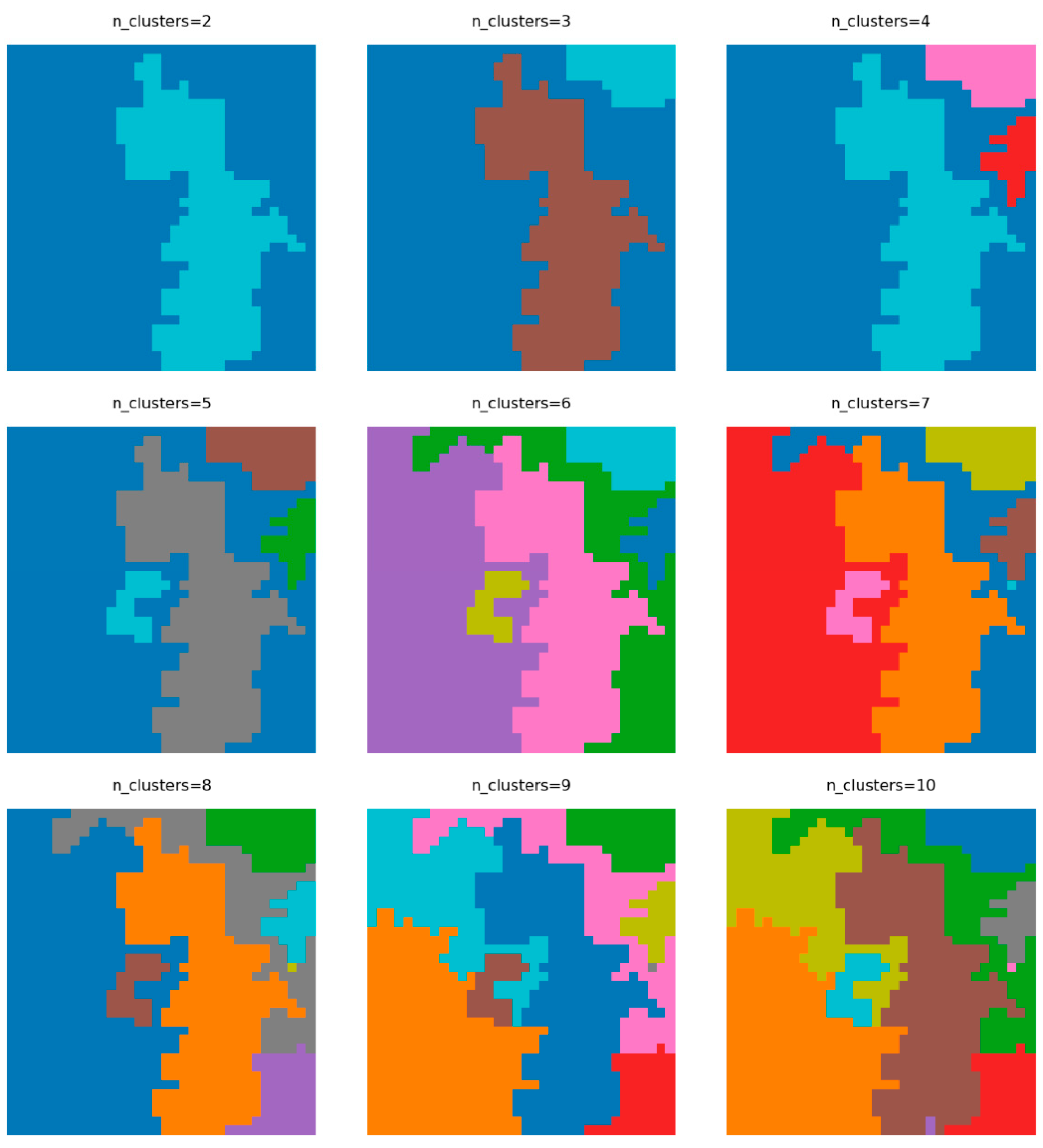
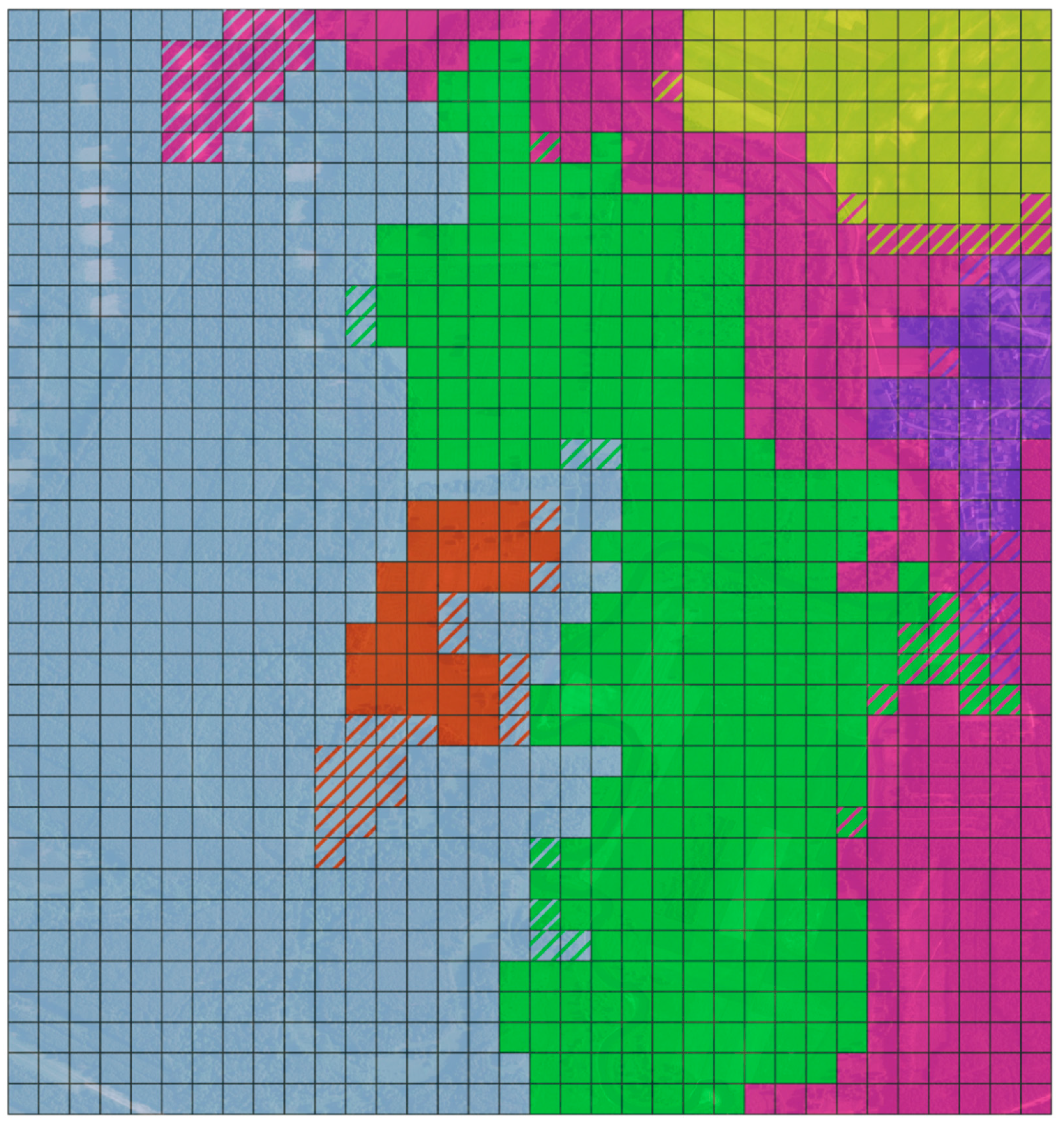
BigBiGAN accompanied by hierarchical clustering can be effectively used as a building block of an unsupervised orthophoto segmentation pipeline. The results of performing this procedure on a test orthophoto (see Figure 9) proves that the solution is powerful enough to divide the area into a meaningful predefined number of regions. Particularly noteworthy is the precise separation of forests, arable lands, and build-up areas. There is also room for improvement. Currently, the network is not capable of segmenting out tree felling areas located in the northwest and the river channel, which would be very beneficial from the point of view of landscape analysis. Furthermore, it also incorrectly combined pastures and arable lands. The main drawback of this method is the need to predefine the number of clusters. What is more, when increasing the number of clusters, artifacts started to occur, and the algorithm predicted small areas that were not identified as distinct regions in the ground truth image (Figure 8, n clusters = 7–10). Further analysis of latent codes and features that they represent is needed to understand the origin of this issue.

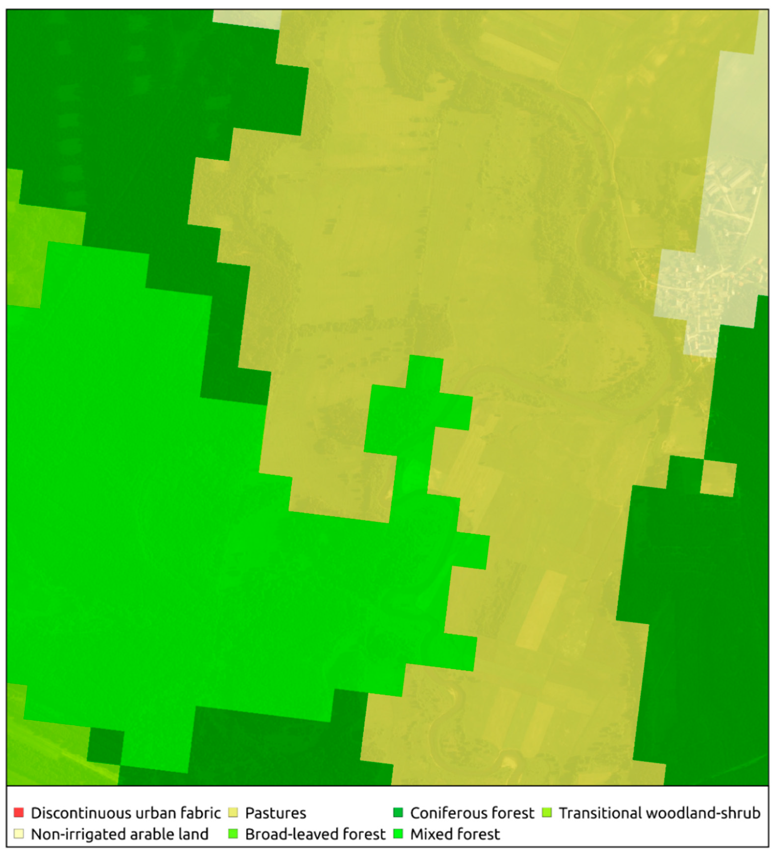
BigBiGAN clustering procedure results resemble, to some extent, the segmentation of the area performed during the Corine Land Cover project in 2018 (Figure 10). It is interesting that the proposed GAN procedure shows a better fit with the boundaries of individual areas than CLC. Nevertheless, CLC has a great advantage over the result generated using GAN, i.e., each tile possesses information about the land cover types that it represents. CLC land cover codes are consistent across all areas involved in the study, which makes this dataset very useful in terms of even sophisticated analysis. This does not mean, however, that the GAN cannot be rearmed to carry information about the land cover types. In the initial BigGAN paper, the authors proposed a solution to enrich each part of the neural network with a mechanism that would enable working with class embeddings [44]. The authors did not use the aforementioned solution to maintain the unsupervised nature of the procedure. An interesting solution would be to compare the latent codes of patches located within different regions to check how similar they are and use this information to join similar, distant regions. To achieve this, a more advanced dataset is needed to cover a larger area and prevent undersampling of occurring less frequently but spatially significant features. Comparison with CLC is also interesting due to the differences in the creation of both sets. CLC is prepared using a semi-supervised procedure that involves multiple different information sources. In contrast, the GAN approach utilizes only orthophotos and is fully unsupervised. Another interesting approach would be to utilize Corine Land Cover (CLC) as the source of model labels and retrain the network to also possess the notion of land cover types. This way, we would gain an interesting solution that would offer a way of producing CLC-like annotations in different precision levels and using different data sources.

5. Conclusions

Generative adversarial networks are a powerful tool that definitely found their place in both geographical information systems (GIS) and machine learning toolboxes. In the case of remote sensing imagery processing, they provide a data augmentation mechanism of creating decent quality artificial data samples, enhancing, or even fixing existing images, and also can actively participate in feature extraction. The latter gives the researchers access to new information encoded in the latent space. During the research, authors confirmed that the bidirectional generative adversarial network (BigBiGAN) encoder module can be successfully used to compress RGB orthophoto patches to lower-dimensional latent vectors.

The encoder performance was assessed indirectly by evaluating the network reconstruction capabilities. Pixel-wise comparison between ground truth and reconstruction output yielded the following results: mean absolute error (MAE) 27.213, structural similarity index (SSIM) 0.942, peak signal-to-noise ratio (PSNR) 42.731, and Fréchet inception distance (FID) 86.36 ± 7.28. Furthermore, the encoder was tested by utilizing output latent vectors to perform geospatial clustering of a chosen area from the Pilica River region (94% patch-wise accuracy against manually prepared segmentation mask). The case study proved that orthophoto latent vectors, combined with georeferences, can be used during spatial analysis, e.g., in region delimitation or by producing reliable segmentation masks.

The main advantage of the proposed procedure is that the whole training process is unsupervised. The utilized neural network is capable of discovering even complex spatial features and code them in the network underlying latent space. In addition, handling relatively lightweight latent vectors during analysis rather than raw orthophoto proved to significantly facilitate the study. During processing and analysis, there was no need to possess a real image (37MB) but only a recipe to compute in on the fly (3MB). The authors think this feature has great potential in the commercial application of the procedure to lower disk space and network transfer requirements when processing large remote sensing datasets.

On the other hand, the presented method is substantially difficult to implement, configure, and train; it is prone to errors and is demanding in terms of computation costs. To achieve a decent result, one must be ready for a long run of trials and errors mainly related to tuning the model and estimating the required dataset size. Regarding latent vectors, authors have identified a major flaw related to the lack of possibility to precisely describe the meaning of each dimension. The main disadvantage of the proposed procedure is that the majority of steps during the evaluation of the model involves human engagement.

The authors are certain that utilizing BigBiGAN on a more robust and rich dataset, like multispectral imagery, backed by digital terrain model (DTM) and at the same time working on reducing the internal complexity of the network to enable processing larger patches will result in a handful of valuable discoveries. The main focus of the research team in the future will be the verification of the proposed method on a greater scale. Future work will involve performing geospatial clustering of latent codes acquired for all Polish geographic regions and presenting the comparison between classically distinguished regions and their automatically generated counterparts.