Exploring the Suitability of UAS-Based Multispectral Images for Estimating Soil Organic Carbon: Comparison with Proximal Soil Sensing and Spaceborne Imagery

Abstract

Soil organic carbon (SOC) is a variable of vital environmental significance in terms of soil quality and function, global food security, and climate change mitigation. Estimation of its content and prediction accuracy on a broader scale remain crucial. Although, spectroscopy under proximal sensing remains one of the best approaches to accurately predict SOC, however, spectroscopy limitation to estimate SOC on a larger spatial scale remains a concern. Therefore, for an efficient quantification of SOC content, faster and less costly techniques are needed, recent studies have suggested the use of remote sensing approaches. The primary aim of this research was to evaluate and compare the capabilities of small Unmanned Aircraft Systems (UAS) for monitoring and estimation of SOC with those obtained from spaceborne (Sentinel-2) and proximal soil sensing (field spectroscopy measurements) on an agricultural field low in SOC content. Nine calculated spectral indices were added to the remote sensing approaches (UAS and Sentinel-2) to enhance their predictive accuracy. Modeling was carried out using various bands/wavelength (UAS (6), Sentinel-2 (9)) and the calculated spectral indices were used as independent variables to generate soil prediction models using five-fold cross-validation built using random forest (RF) and support vector machine regression (SVMR). The correlation regarding SOC and the selected indices and bands/wavelengths was determined prior to the prediction. Our results revealed that the selected spectral indices slightly influenced the output of UAS compared to Sentinel-2 dataset as the latter had only one index correlated with SOC. For prediction, the models built on UAS data had a better accuracy with RF than the two other data used. However, using SVMR, the field spectral prediction models achieved a better overall result for the entire study (log(1/R), RPD = 1.40; R²_CV = 0.48; RPIQ = 1.65; RMSEPCV = 0.24), followed by UAS and then Sentinel-2, respectively. This study has shown that UAS imagery can be exploited efficiently using spectral indices.

1. Introduction

Soil organic carbon (SOC) content is one of the leading indicators for soil state assessment. Therefore, a thorough and timely observation of SOC content with effective techniques is needed to better understand the function of soil within the carbon cycle universally [1,2]. However, numerous drawbacks, including complex and unpredictable environmental conditions, and numerous soil-forming conditions, limit the efficiency and performance of their estimation. Due to these unfavorable factors, the mapping of SOC and its attributes requires time and money [2,3]. Therefore, there is a global surge toward the need for fast and less costly techniques for efficient quantification of SOC content.

In response to these challenges, the emersion of proximal soil sensing (PSS) and remote sensing (RS) approaches is described as a useful detection tool for evaluating and analyzing several soil parameters including SOC [4,5,6]. For proximal sensing, a physical contact is needed to obtain signal from the target using the spectrometer sensor (within 2m apart) [7]. Whereas, for remote sensing (RS), electromagnetic radiation is used to obtain, without physical contact data or occurrence [8]. Spectroscopy (visible near-infrared (vis-NIR)) under PSS is also classified as a useful tool for the accurate quantification, in laboratory [2,9,10], and in the field [11,12,13] of SOC content with limited resources. Its approach for soil assessment started in the years 1960 to 1980 [14] and intensified between 1990–2000s [15]. Research into vis-NIR spectroscopy approaches within soil science has also increased rapidly in the last couple of decades [16,17]. For example, with infrared spectroscopy, a sole spectrum can allow the identification of contrasting soil constituents concurrently [5]. Nevertheless, when using spectroscopy, one of the suggestions is that the accumulation of an established soil component is linear to a mixture of absorption properties within the spectral range, also the issue where organic and inorganic molecules can absorb at wavelengths beyond 2000 nm cannot be ignored [18,19]. According to Mulder et al. [20], qualitative and quantitative information on soil variables and soil classification can be collected in a cost-effective approach using RS. For example, it is difficult to disregard the short revisit duration of the Sentinel-2 imagery and the large quantity of the data set generated that is available and can also be freely downloaded [21]. In addition, the spectral composition of the soil can be calculated affordably and conveniently, thus providing a trade-off between cost and precision [22]. Nevertheless, in terms of detailed large-scale site monitoring, enhanced results classification, and data reduction, remote sensing has an advantage over PSS [23]. For measurement, RS methods can be categorized into two main types, namely spaceborne (e.g., use of satellites) and airborne (either aircraft or drone). However, aerial surveillance, employing imagery collected by satellites, manned aircraft and unmanned aerial vehicles (UAVs)(actual aircraft (Drone) itself), is one of the most commonly used RS techniques [24]. Airborne imaging can provide a more precise mapping of the variability found in agricultural fields. Even from a single flight mission, the information produced can cover wide areas because the aircraft has adequate flight duration [25]. Moreover, airborne sensors can also provide site segmentation data based on soil heterogeneity, while expanding existing soil property datasets to support digital soil mapping [20]. Spaceborne remotely sensed imagery, on the other hand, has an enormous potential as an enabling instrument for generating soil profile maps, due to the relation that can be created between the soil’s complex chemical bonds and electromagnetic radiation. For example, with the introduction of the first satellites in the 1980s, optical satellite (multispectral) imagery was widely utilized for a comprehensive SOC assessment [26]. However, the traditional airborne and satellite remote sensing frameworks where most sensors (e.g., multispectral, hyperspectral, etc.,) are mounted, have not always satisfied the researchers’ and environmental demands [27]. In case of environmental applications, some of these platforms are prone to several issues like high cost and especially poor spatial and temporal resolution. Satellite data can be very appealing because of its broad spatial coverage including inaccessible areas that were historically too remote or too harmful to reach while using traditional aerial photography [28,29]. Nevertheless, issues such as low resolution and excessive noise while using Hyperion satellites [11] and the 16-day Landsat-8 revisit period suggest that the available options for time series research and bare soil observation may be minimal [30,31]. According to Crucil et al. [32], some of the above-mentioned issues with spaceborne still remain unresolved even with the emersion of new satellites, especially Sentinel-2. Moreover, Sentinel-2 data may even have to undergo several pre-processing steps which could affect its prediction capability of soil properties.

Although remote sensing imagery (e.g., hyperspectral images) offers detailed bare soil spectral data, the effects posed by some RS factors, especially the soil water content and dissolved organic material within the soil, cannot be ignored [33,34]. Consequently, one or more appropriate spectral indices could be necessary to help limiting the effect posed by the above listed factors on RS imagery [33,35,36]. For examples, Jin et al. [37], reported improved results by using several indices to predict soil organic matter.

Over the past decade, the development of UAS, also known as unmanned aircraft system, has made it possible to obtain valuable data that have been beneficial to determine spatial variability within soil properties [27], especially SOC [38] that would have been difficult to identify utilizing conventional frameworks for RS. UAS can be categorized depending on the nature of its wings either as non-movable (non-mobile) or movable (mobile), with the non-mobile wings typically having higher speed and greater duration, while the mobile wings can offer greater maneuverability. UAS appear as versatile platforms with the potential to augment RS survey collected from spaceborne or manned aircraft [27]. Although UAS cannot compete based on the spatial coverage with satellite imagery, they offer unparalleled spatial and temporal resolutions unrivalled by satellite alternatives [39]. Because of its spatial-temporal advantage, the UAS-based approach can provide greater return time by providing high performance rates for many flights throughout the day and monitoring processes at a very high spatial and temporal resolution [40]. UAS technology is now mainstream and cost-effective and is being utilized for a broad variety of environmental applications, for example, estimating evapotranspiration, or assessing water stress for sustainable agriculture and precision agriculture [41,42,43,44,45]. For monitoring/quantifying of SOC in agricultural or arable lands, UAS borne imagery has received attention from some researchers [32,38,46], but most of these studies were focused on fields with rather high SOC concentration. This implies that a field low in SOC has not yet been explored. Although UAS has numerous advantages, it is also prone to problems such as restricted payload, short flight endurance, and difficulties in maintaining flight speed and stability during heavy winds and turbulence [47]. However, in terms of new technological advancement, most of the technical problems of the UAS could be solved by collaboration involving environmental experts and UAS engineers [48].

Nevertheless, it is worth mentioning that the Association for Unmanned Vehicle Systems International (AUVSI) has estimated that in the coming years, about 80% of UASs will be used for agricultural activities [43]. UAS sales in Germany, for example, approached 400,000 units in 2017 and were projected to grow to over a million by the end of 2020. Moreover, UAS sales doubled in the US in the same year, with an increase of 117 percent compared to the previous year [49]. Finally, as reported by Kriehn [45], in 2019, there were 900,000 registered UAS drones in the United States, with about 17 percent being used for agriculture.

Clearly, the use of UAS is increasing rapidly, which calls for further studies to assess and enhance its prediction capability for soil properties, especially SOC. Although there have been some studies on both Sentinel–2 and UAS imagery for exploring SOC content, the focus has mainly been on fields with high SOC content. This study aims to focus on a field that is poor in SOC and, importantly, to verify the effect of spectral indices from UAS data (which is rarely used by researchers), as remote sensing data are vulnerable to many disturbing external environmental parameters. To the best of our knowledge, no studies have evaluated the capability of UAS for the agriculture fields with a low amount of SOC when coupled with spectral indices. Therefore, this study’s primary objective is to evaluate and compare UAS monitoring capabilities and estimation of SOC with those obtained from spaceborne (Sentinel-2) and proximal soil sensing (field spectroscopy measurements) on an agricultural field low in SOC content as well as verifying the effect of soil and vegetation indices. The spatial SOC distribution map will also be computed for the various sensors used in reference to the laboratory SOC measured values.

2. Materials and Methods

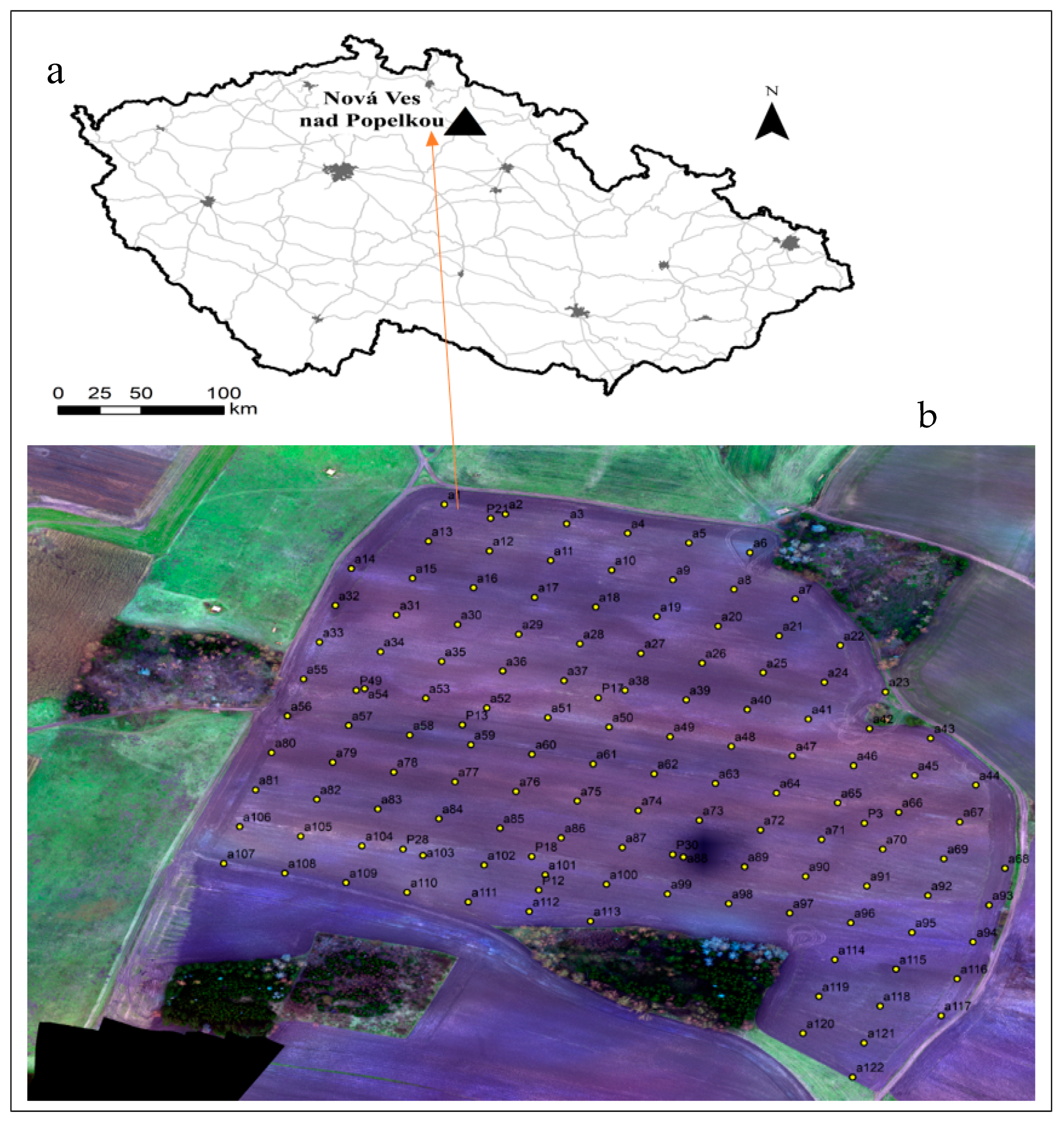
2.1. Study Area

The site used for this study is a 22 ha agricultural land situated at Nová Ves nad Popelkou (50.310° N, 15.240° E), in the Liberec Region (Figure 1), in the Czech Republic. The region has consistent mean windspeeds of 6 km/h, a humidity of 74% with an average altitude of 185 m a.s.l. The region is predominantly agricultural and is dedicated to winter and spring cereals and is dominated by dissected relief with side valleys and toe-slopes. Local prevalent soils types are mainly Cambisols and Stagnosols on crystalline and sedimentary rocks according to the World Reference Base for Soil Resources (IUSS Working Group WRB, 2014).

2.2. Soil Sampling and Field Spectral Measurement

A sampling grid method comprising 130 sampling points spread across the whole field was used, as shown in Figure 1. Prior to the actual site survey, those sampling points (130) were generated and identified in the field employing GeoXMM. (Trimble Inc., Sunnyvale, CA, USA) receiver with an accuracy of 1 m. The field spectra were measured instantly in the field on 6 May 2019 using an ASD Field Spec III Pro FR spectroradiometer (ASD Inc., Denver, CO, USA) across the 350–2500 nm wavelength range. The spectroradiometer spectral resolution was 2 nm for the region of 350–1050 nm and 10 nm for the region of 1050–2500 nm. Measurements from four different positions around each of the 130 sampling points were taken, and the average value was used as the field spectral dataset. The spectroradiometer was calibrated before the first scan and after every six measurements, using a white Spectralon TM (Lab-sphere, North Sutton, NH, USA) [50]. Soil samples were also collected from each of those positions (depth 0–20 cm) while the field measurement was underway. Composite samples (approximately 150 to 200 g of soil) were placed into well-labelled bags and transported to the laboratory for further analysis. These samples were then air-dried, gently crushed, and sieved (≤2 mm) and SOC was measured as total oxidized carbon using wet oxidation approach [51]. This process utilized the dichromate redox titration approach and was accomplished in two different sub-steps [52]. That is, the samples were first oxidized with K₂Cr₂O₇ and the solution was then potentiometrically titrated with ferrous ammonium sulphate.

2.3. Remote Sensing Imagery

The remote sensing data used were the Sentinel-2 and UAS imagery at different resolution.

Table 1. Key radiometric features of multi-spectral sensors shown in this analysis.

Features of the Sensor	Sentinel-2	Trinity F90 Fixed-Wing Drone
	[53]
Mission	Spaceborne	UAS
Sensor type	Push-broom	MicaSense Altum dual sensor
Spectral bands	13	9
Used spectral bands	10	6
Spectral range	9 vis-NIR	9VNIR
	3 SWIR
FWHM (nm)	20–200
SNR	129 (444) nm	32 (475) nm
(typical)	154 (497) nm	14 (531) nm
	168 (560) nm	27 (560) nm
	142 (664) nm	16 (650) nm
	117(704) nm	14 (668) nm
	89 (740) nm	10 (705) nm
	10 (783) nm	12 (717) nm
	174 (843) nm	57 (842) nm
	72 (865) nm	thermal infrared 8–14 um
	114 (943) nm
	50 (1377) nm
	100 (1613) nm
	100 (2200) nm
GSD	10/20/60 m	Variable
(spatial resolution)		(8.8 cm)
Positional accuracy	12 m	3 m
Acquisition date	10 June 2019	25 November 2019

UAS: unmanned aircraft system; vis-NIR: visible and near-infrared; FWHM: full width at half maximum; SNR: signal-to-noise ratio (Wavelength mentioned); SWIR: short-wave infrared; GSD: ground sampling distance.

provides an overview of their individual missions’ characteristics.

2.3.1. UAS Multispectral Imagery

Multispectral data were acquired using a Trinity F90 fixed-wing drone with a MicaSense Altum dual sensor mounted onboard with two cameras (RGB + Multispectral). The MicaSense Altum dual sensor captures images in six independent spectral bands (multispectral) with the last band being a thermal infrared sensor (Blue 475 nm (B4), Green 560 nm (B5), Red 668 nm (B6), Red edge 717 nm (B7), Near-infrared 840 nm (B8), and Thermal 11 μm (B9)). The RGB sensor also captures images in three bands (red-green-blue) (400–700 nm). This is a high-resolution digital camera that is separated from the multispectral sensor. This implies that the total bands captured by the Trinity F90 were nine. The location of the on-board Global Navigation Satellite System (GNSS) and Inertial Navigation Unit has been saved in the metadata files using the Exchangeable Image File Format (EXIF). The camera is equipped with a sun sensor that gathers information about the light conditions and saves the radiant flux data produced in the EXIF format. The image was acquired on 25 November 2019 at Nová Ves nad Popelkou in a clear sky condition. The flight plan was prepared using a QBase 3D mobile app (mission planning software), this served as the primary interface between the user and the UAS device. QBase 3D offers real-time information, such as altitude, distance, battery life about the UAS, and mission telemetry data that provide the operator with updated information about the flight at all times. The flight height was 190 m and the spatial resolution was 8.8 cm, covering an area of 31 ha. We also ensured that we had sufficient batteries for the total flight duration over the entire study field. The images were captured automatically, and the calculated position was consistent with 85% front and 75% side overlap. The images were accurately oriented, 3D model was extracted, the digital elevation model (DEM) was calculated based on the generated cloud point (during the flying period), and orthorectified images were calculated and then exported as one mosaic in GeoTIFF file in EPGS 4326—Geographic coordinates on WGS-84 ellipsoid. Before generating this orthophoto, calibration is performed. The obtained image (before calibration) is already in the reflectance format, however, the actual reflectance values are obtained by dividing each band by 32,768 to get the values normalized in the interval between 0 and 1. The 32,768 is the band center value which represents 100 percent of reflectance. For geometrical correction, the ground-based points and the Differential Global Positioning System (DGPS) were used while for both radiation correction and transformation of reflectance, the Gray Scale Correction method was utilized. AgiSoft Metashape Professional 1.5.0 (AgiSoftLLC, St. Petersburg, Russia), photogrammetric processing was used. The software’s consistent performance in photogrammetric processing has been demonstrated in previous studies [54]. In order to differentiate bare soil areas, the Normalized Difference Vegetation Index (NDVI) was employed to mask a threshold of 0.2. The R software (R Development Core Team, Vienna, Austria) was used for all other data processing. For this study, it was only the multispectral section (Trinity F90) with six bands that was used for further analysis.

2.3.2. Sentinel-2 Imagery

The extracted cloud-free Sentinel-2B imagery used for this study was carried out at the European Space Agency’s Copernicus Open Access Hub on 10 June 2019. The Sentinel-2 mission consists of two similar satellites: Sentinel-2A, and Sentinel-2B, respectively. Each satellite has a Multi-Spectral Instrument (MSI) that generates images of the earth. The Sentinel-2 images are processed to Level-1C, which implies that they have been ortho-corrected, map-projected images containing top-of-the-air reflectance data. This image will need further pre-processing by the user, but the level 2A Sentinel-2 imagery can be used instantly because its dataset has been processed by the suppliers using Sen2Cor processor. These processes include geometric, radiometric, and atmospheric corrections. For this study the level 2A Sentinel-2 imagery was used. The Sentinel-2 image consists of 13 spectral bands. These spectral bands range from the visible and near infrared (vis-NIR) to the short-wave infrared (SWIR). They include four bands at 10 m resolution ((B2, 490 nm), (B3, 560 nm), (B4, 665 nm), (B8, 842 nm)); six bands at 20 m resolution ((B5, 705 nm), (B6, 740 nm), (B7, 775 nm), and (B8A, 865 nm); 2 SWIR large bands, (B11, 1610 nm) and (B12, 2190 nm). Finally, three bands at 60 m resolution ((B1, 443 nm), (B9, 940 nm), and (B10, 1380 nm)). Before downloading, all the 13 band were resampled to 10 nm using the SNAP software (by pixel resolution). With the exception of B1, B9, and B10 that were omitted, all the remaining bands were used for this study. The Sentinel-2 user handbook [55] describes the whole protocol.

Soil optical properties can be influenced by certain factors such as soil water content, mineral composition, and organic matter content [37]. Therefore, nine calculated spectral indices have been applied to both Sentinel-2 and UAS datasets as independent variables, anticipated to enhance the prediction capability of the datasets. The added spectral indices were Colour Index (CI), Normalized Differences Vegetation Index (NDVI), Infrared Percentage Vegetation Index (IPVI), Normalized Difference Red Edge (NDRE), Soil Adjusted Vegetation Index (SAVI), Vegetation (V), Normalized Difference Vegetation Index (GNDVI), Difference Vegetation Index (DVI), and Brightness Index (BI). The equations used to determine these indices are shown in

Table 2. Indices derived from Sentinel-2 and UAS spectra.

Index	Definition Based on Sentinel-2	Definition Based on UAS	References
CI	$\frac{B4-B3}{B4+B3}$	$\frac{B6-B5}{B6+B5}$	Pouget et al. [56]
NDVI	$\frac{B8-B4}{B8+B4}$	$\frac{B8-B6}{B8+B6}$	Rouse et al. [57]
IPVI	$\frac{1}{2}\left(NDVI+1\right)$	$\frac{1}{2}\left(NDVI+1\right)$	Crippen [58]
NDRE	$\frac{B8-B5}{B8+B5}$	$\frac{B8-B7}{B8+B7}$	Barnes et al. [59]
SAVI	$\frac{\left(B8-B4\right)\ast \left(1+L\right)}{B8-B4+L}$ L = 0.5	$\frac{\left(B8-B6\right)\ast \left(1+L\right)}{B8-B6+L}$ L = 0.5	Huete [60]
GNDVI	$\frac{B8-B3}{B8+B3}$	$\frac{B8-B5}{B8+B5}$	Gitelson et al. [61]
DVI	B8-B4	B8-B6	Richardson and Wiegand [62]
BI	$\frac{\sqrt{\left(B4\ast B4\right)+\left(B3\ast B3\right)}}{2}$	$\frac{\sqrt{\left(B6\ast B6\right)+\left(B5\ast B5\right)}}{2}$	Escadafal [63]
V	$\frac{B8}{B4}$	$\frac{B8}{B6}$	Jordan [64]

Sentinel-2 (B3: Green, B4: Red, B5: Red Edge, B8: NIR); UAS (B5: Green, B6: Red, B7: Red Edge, B8: NIR).

. SNAP was used to obtain bare soil pixel values at sampling locations.

2.4. Data Pre-Processing Approaches

The initial field spectral range was 350–2500 nm; however, the noisy segments of 350–399 nm were removed prior to spectra treatment, retaining only 400–2500 nm range. The field spectra and the other two dataset (UAS and Sentinel-2) were then subjected to the following set of pre-processing techniques: discrete wavelet transformation (DWT), standard normal variate (SNV), logarithmic transformation (log(1/R)), as well as the combination of DWT with SNV (DWT + SNV) and with log(1/R) (DWT + log(1/R)). The DWT is a known technique for signal smoothing and/or noise reduction. This function was determined using the wavelet package in the R software [65]. Also, all other pre-treatment algorithms have been computed using the R software.

2.5. Modelling and Prediction Assessment

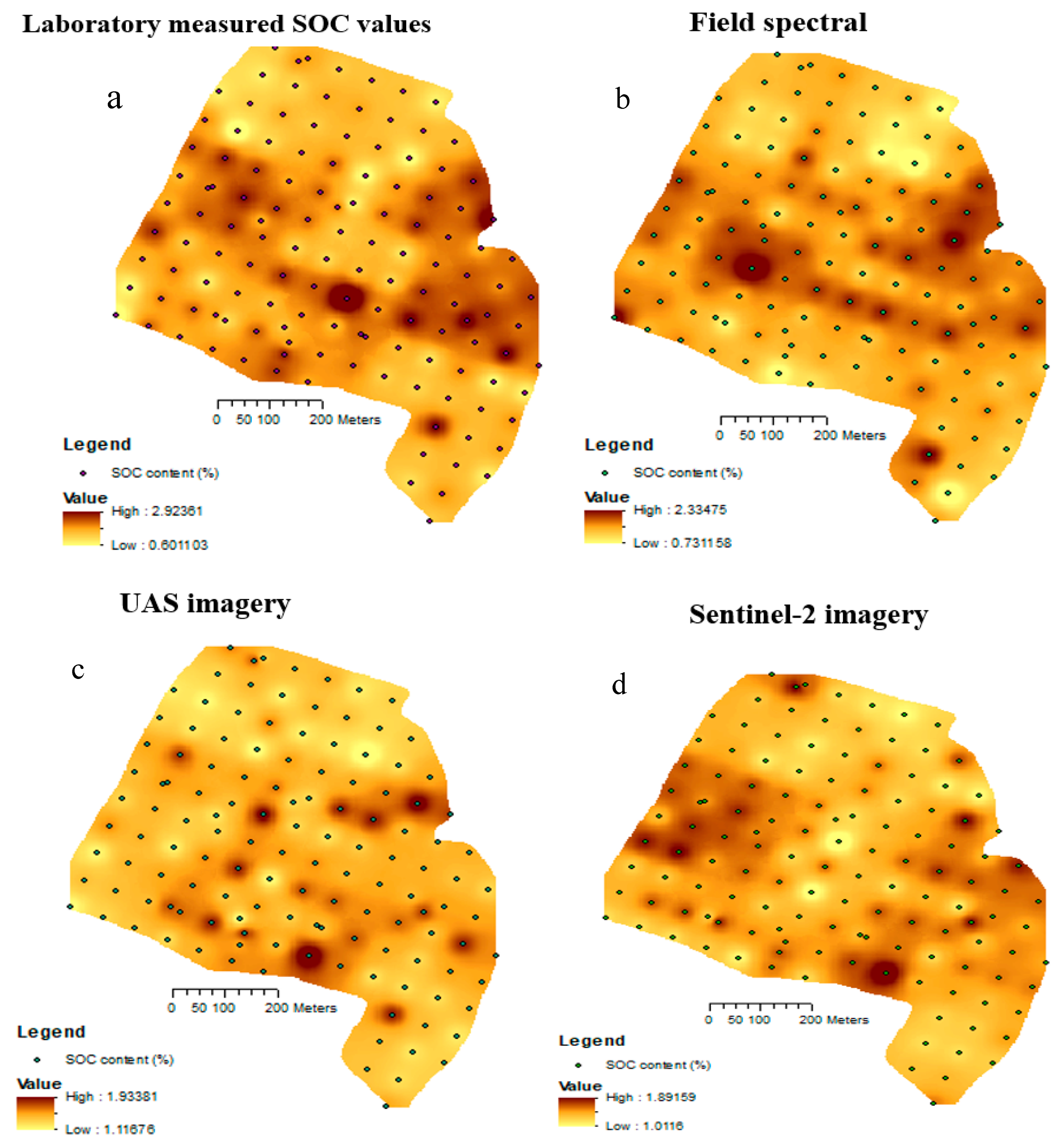
The spectra obtained from Sentinel-2 and UAS sensors, including the determined spectral indices, were each linked to the SOC determined in the laboratory using collected soil samples from the field. For the field data, the spectral measurement in the field was used. The above-mentioned datasets were used to build SOC predictive models. The spatial resolution for the UAS remains the same (8.8 cm). Two separate multivariate models were evaluated for all spectral data, namely random forest (RF) and support vector machine regression (SVMR). SVMR is a nonlinear algorithm used for regression and classification processes with a set of related supervised learning algorithms, which has an excellent ability to be a universal predictor of any multivariate function to any defined degree of accuracy. Even if the discriminant feature gathered is based on minimal data, the independent test set’s prediction error can still be small. RF is also a technique for classification and regression. RF belongs to the ensemble machine learning algorithm family that predicts a soil parameter response from a set of predictors that could be a training data matrix. This is done by creating and aggregating multiple decision trees. RF also adjusts splitting by picking the best split from a randomly chosen subset of predictors [66]. In multivariate regression models, spectral reflectance data were used as predictor variables and selected soil parameters data as output responses. The model output was evaluated for each regression procedure by five-fold cross-validation of the training set (75%) and the testing set of 25% of the samples using SVMR and RF modelling techniques. The prediction accuracy was evaluated by index of determination (R²_CV), the ratio of performance to interquartile range (RPIQ), the root mean square error of prediction (RMSEPcv) of the 5-folds cross-validation, and the ratio of performance to deviation (RPD). The RPD was determined as an auxiliary indicator of model reliability as the ratio of the RMSEPcv to the standard data deviation. The larger the RPD, the better the model for prediction. Prior to evaluating the predictive models, the normality of the distribution of the SOC contents was examined (skewness <1).

A correlation matrix was also calculated to visualize the relationships between the three datasets and their parameters (indices) with SOC (examine which dataset is more correlated or significantly correlated). For the remote sensing data set (UAS and Sentinel-2), this was done between SOC and their bands and indices. However, for the field spectra, the correlation was made with SOC using only selected wavelengths (based on UAS and Sentinel-2 wavelengths) due to the enormous amount of spectral data available (350–2500 nm).

For a visual comparison of SOC spatial distribution predicted by models based on different data and laboratory measurement, SOC maps were created using the inverse distance weighting (IDW) interpolation method.

3. Results

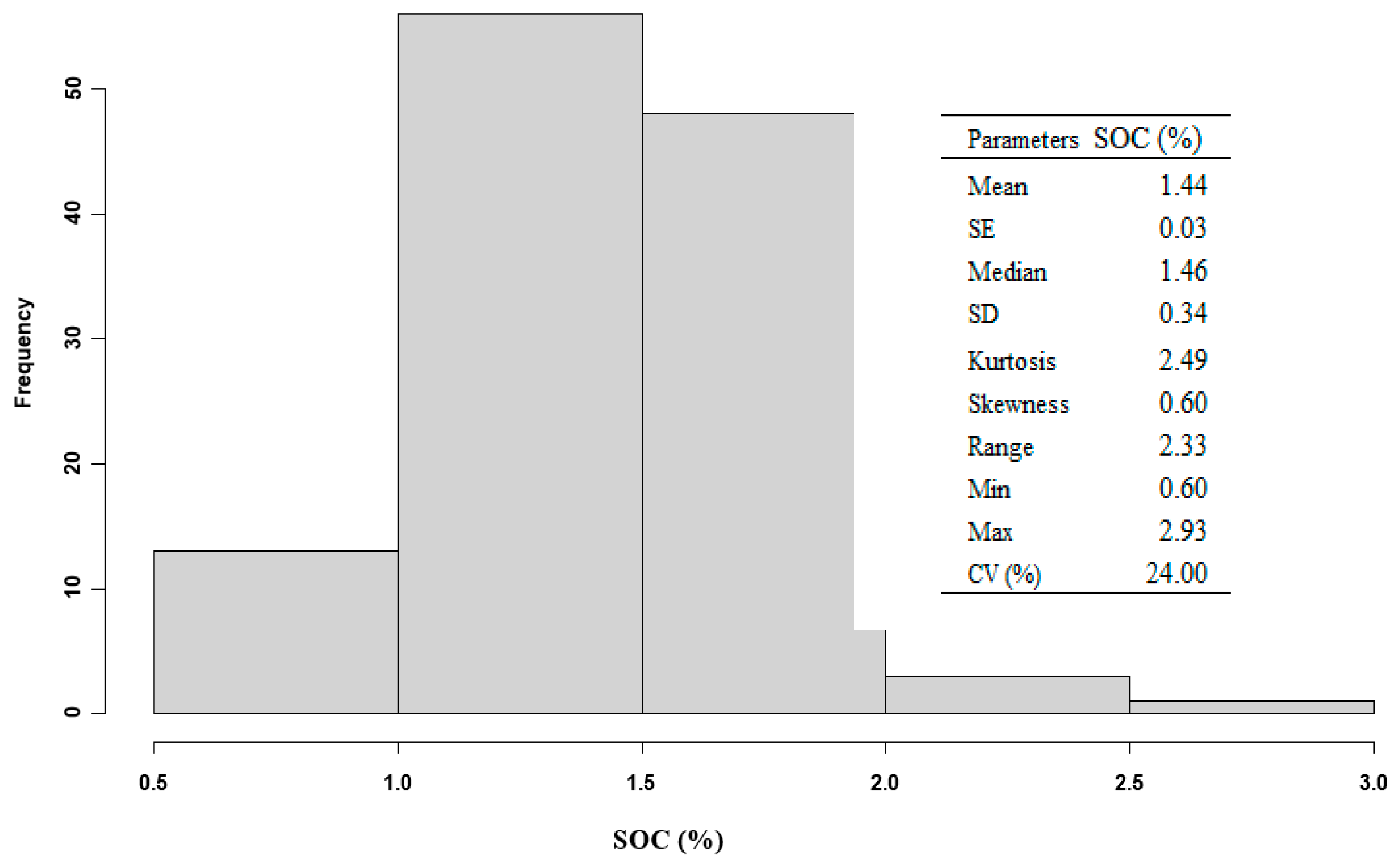
3.1. Soil Organic Carbon (SOC) Frequency Histogram and Descriptive Statistics

Figure 2 is a frequency histogram and a statistics summary of SOC characteristics in soil samples within the study area comprising standard deviation (SD), coefficient of variation (CV), minimum, maximum, mean value, skewness, and standard error (SE). The statistical distribution of the SOC within the sample site was positively skewed. A visual inspection of the SOC histogram showed that the value distribution (tail region) has shifted to the left side. Generally, the overall result signifies a low to medium SOC content of the area.

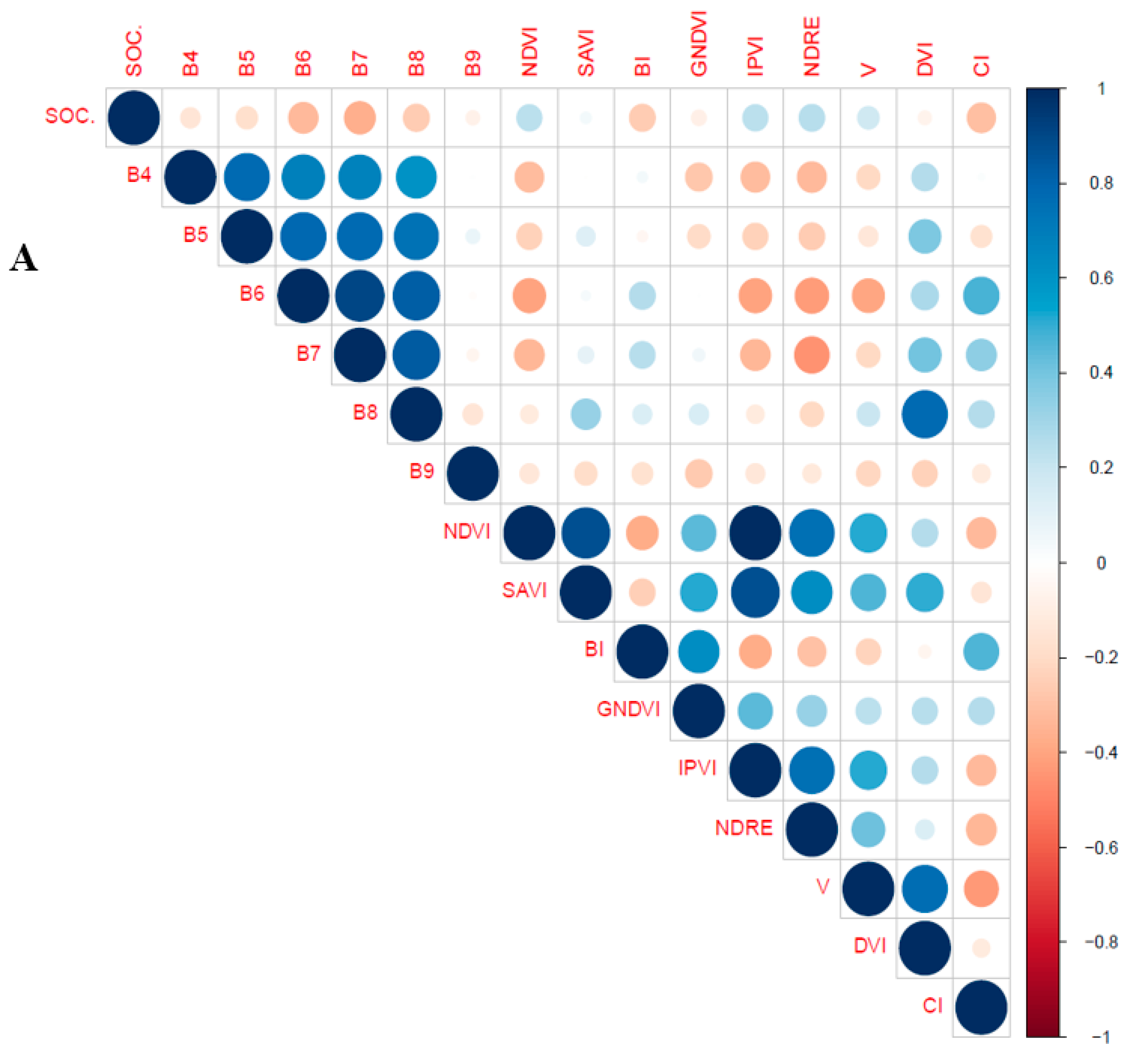
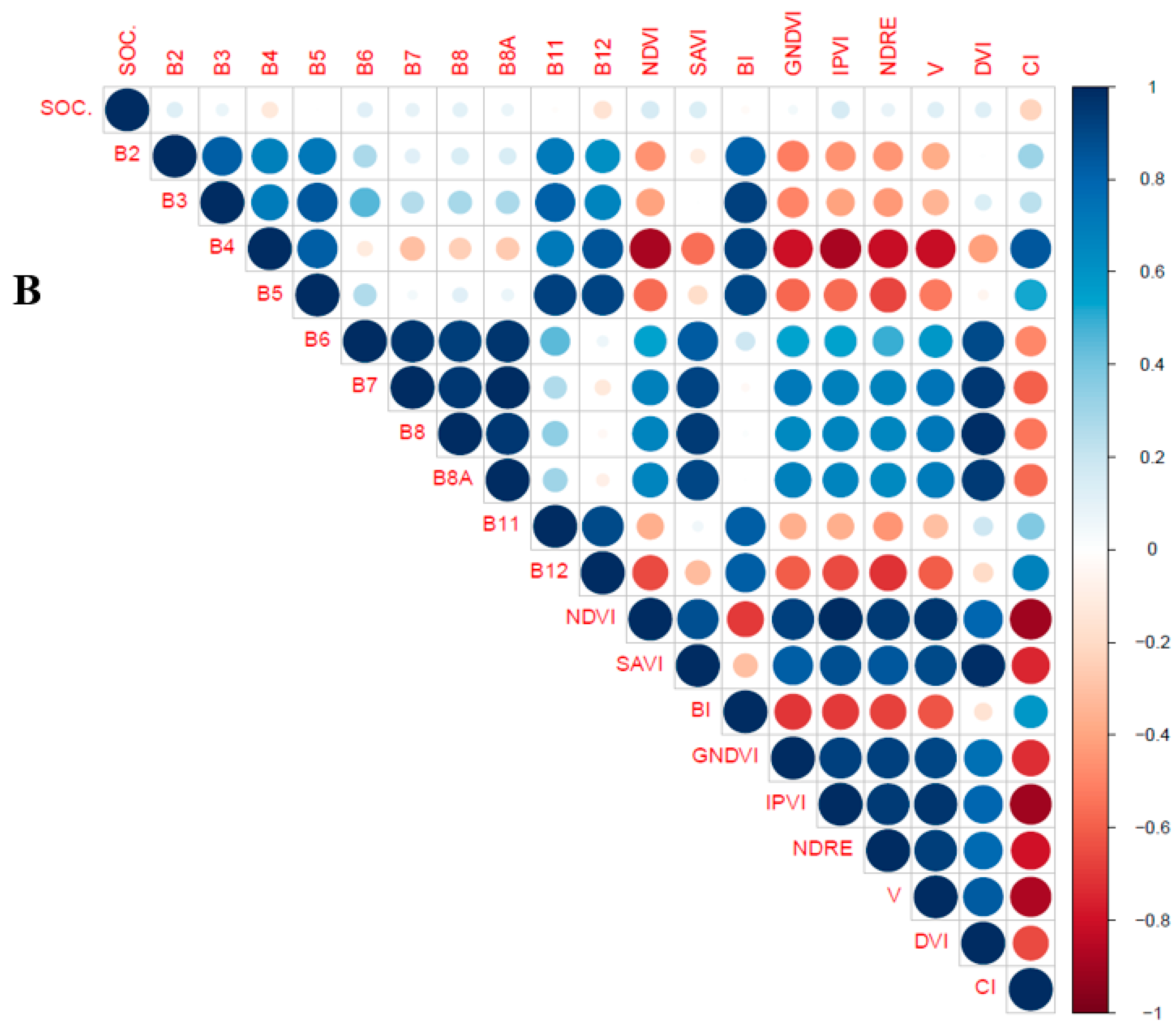
3.2. Correlation of SOC with Reflectance Bands and Spectral Indices for Sentinel-2 and UAS Datasets

To visualize the differences between UAS, Sentinel-2 imagery datasets and the calculated indices (for each dataset) within the study area, correlation matrices between their parameters (bands and indices) and SOC were built (Figure 3). The correlation matrices helped to determine among the datasets strong or significant correlations (in both positive and negative directions) so as to identify which spectral bands or indices are the key determinants in the prediction of SOC. For the UAS dataset, the most significant correlations were found between SOC and CI, band 7 and band 6, followed by NDVI, NDRE, IPVI, and BI. For the Sentinel-2 spectral bands, it was only CI that provided significant correlation with SOC. Although, neither dataset was strongly correlated with SOC, there were strong correlations between some of the bands and indices.

3.3. Correlation between SOC and Selected Wavelength of Field Spectra

Figure 4 displays the correlation matrix of SOC with selected wavelengths of field spectra. These wavelengths were selected using the wavelength values that were similar or closer to that of UAS and Sentinel-2 bands. Considering all selected wavelengths, the strongest significant correlations between SOC and field spectra were obtained from 443, 665, 668, 705, and 717 nm while the remaining wavelengths showed good correlations. Although strong correlation was seen between all selected wavelengths (among each other), there were no strong correlation witnessed between SOC and the selected wavelengths.

3.4. Prediction of SOC Using UAS, Sentinel-2 and Field Spectra Data Sets

The prediction results (

Table 3. Statistics of the fivefold leave-group-out cross-validation for field spectra, UAS and Sentinel-2 using random forest (RF) and support vector machine regression (SVMR) with different pre-processing methods.

	UAS				Sentinel-2				Field Spectra
					RF
Treatment	RPD	R2cv	RPIQ	RMSEPcv	RPD	R2cv	RPIQ	RMSEPcv	RPD	R2cv	RPIQ	RMSEPcv
Raw	1.05	0.11	1.24	0.32	1.04	0.04	1.22	0.32	0.99	0.05	1.14	0.34
DWT	1.13	0.27	1.36	0.29	1.02	0.02	1.2	0.33	1.02	0.08	1.18	0.33
SNV	1.00	0.14	1.19	0.34	0.96	0.15	1.27	0.35	1.12	0.22	1.31	0.3
SNV + DWT	1.01	0.03	1.22	0.33	1.02	0.01	1.23	0.33	1.08	0.18	1.28	0.31
Log(1/R)	1.04	0.22	1.31	0.32	1.02	0.05	1.29	0.33	1.01	0.06	1.14	0.33
Log + DWT	1.10	0.17	1.27	0.3	1.01	0.01	1.18	0.33	1.02	0.05	1.14	0.33
					SVMR
Raw	1.01	0.11	1.18	0.33	1.07	0.15	1.27	0.31	1.21	0.36	1.44	0.28
DWT	1.05	0.14	1.16	0.32	1.03	0.11	1.13	0.33	1.23	0.35	1.44	0.27
SNV	1.06	0.22	1.25	0.31	1.08	0.24	1.31	0.33	1.31	0.44	1.53	0.26
SNV + DWT	1.04	0.12	1.12	0.32	1.05	0.11	1.14	0.32	1.35	0.45	1.59	0.25
Log(1/R)	1.09	0.19	1.29	0.31	1.08	0.16	1.28	0.31	1.4	0.48	1.65	0.24
Log + DWT	1.07	0.11	1.15	0.31	1.06	0.12	1.12	0.32	1.33	0.45	1.56	0.25

) showed that the highest prediction accuracy of SOC (RPD = 1.4; R²_CV = 0.48; RPIQ = 1.65; RMSEP_CV = 0.24, for log(1/R)) were obtained with field spectral data using SVMR algorithm. This was followed by UAS (DWT, RF) with RPD = 1.13, R²_CV = 0.27, RPIQ = 1.36, and RMSEP_CV = 0.30, and finally Sentinel-2 (SNV), SVMR) with RPD = 1.08, R²_CV = 0.24, RPIQ = 1.31, and RMSEP_CV = 0.31, respectively. Moreover, other improved result was also obtained using SNV + DWT, log + DWT, and SNV (SVMR) methods with the field spectra and log(1/R) (RF) with UAS.

4. Discussion

Spectroscopy under proximal soil sensing has now become a common way of estimating SOC and other soil parameters because of its high accuracy level compared to the other forms of measurement stated above [7]. In comparison with the other two data sets, namely UAS and Sentinel-2, the field spectra under proximal soil sensing show the best prediction output as expected (RPD = 1.4; R²_CV = 0.48; RPIQ = 1.65 and RSMEP_CV = 0.24, for log(1/R), SVMR). Although the RPD and R²_CV value for this field is not so high, it is comparable to other research findings [67]. Nonetheless, Stevens et al. [25] demonstrated in one of their studies the efficiency of field measurements in comparison to airborne spectroscopy to predict SOC. However, under field measurement, spectroscopy is prone to external environmental conditions, primarily soil moisture, while under laboratory conditions its final output can be influenced by issues such as spectrometer instability, illumination source, detector output, and sample preparation.

Considering the field spectra correlation with SOC using the selected wavelengths based on both UAS and Sentinel-2 bands, it reveals that most of the wavelengths were significantly correlated with SOC compared to the other two datasets. Likewise, almost all selected wavelengths of the field spectra were strongly correlated with each other. This might have accounted for the improved performance of field measurements using vis-NIR spectroscopy approach. However, field spectroscopy inability to cover large spatial areas is one of its major disadvantages. This is because the costs and work and time demands associated with field and laboratory evaluation makes it difficult to undertake soil properties assessment on a vast scale area [68].

The vast frequent data streams generated by satellite sensors can also ensure that soil monitoring and mapping techniques for larger areas can be accurately, rapidly, and effectively established [29,69]. In this study, the accuracy of SOC predictions using Sentinel-2 imagery was the lowest compared with the other two datasets, although the differences were rather small compared to that of the UAS (Table 2). One of the probable reasons for its worst performance could be the low correlation of all Sentinel-2 bands and almost all the calculated indices used with SOC. It could also be presumed that our quest to acquire a cloud-free image which shifted the Sentinel-2 image collection date from early May to June, a likely period for some vegetation to emerge on the field, could have affected the accuracy of Sentinel-2 imagery prediction. For instance, Castaldi et al. [21] attributed the weak output of Sentinel-2 imagery data in their study to the probable influence of maize seedlings on some of the Sentinel-2 bands (wavelengths), highly sensitive to vegetation. This is so because their Sentinel-2 image was collected in May when maize seedlings may have been emerging. According to Bartholomew et al. [70], spectral reflectance form can sometimes be affected because of the apparent existence of fresh or dry vegetation (less than 20%) and therefore the predictive accuracy of soil properties could be affected. Satellite data can be desirable due to its wide spatial coverage, fast revisit time, and the ability to acquire data unaffected by local air traffic restrictions, however, as a result of cloudiness or when parched and bald soil conditions are needed, these predetermined revisit times may not be suitable for adequate temporal coverage [32]. Other challenges for satellite applications are the relatively low image resolution, restricted availability of high-quality temporal and spatial images, primarily as a result of adverse atmospheric conditions and sensor requirements [71]. For example, in Brazil, Friedel et al. [72] utilized spectroscopy techniques and spaceborne (Hyperion satellite) imagery to quantify soil obtained from the tropics. They indicated that because of the presence of shadow within the study area, satellite image efficiency was hampered. In addition, Steinberg et al. [73] evaluated the potential of both airborne and spaceborne (simulated EnMap) imaging spectroscopy for SOC and clay prediction. Their finding was that the airborne imagery revealed a small improvement with regard to the accuracy of prediction compared to the spaceborne domain.

UAS may be a cheaper and more realistic replacement to satellites, general aviation aircraft and even ground spectroscopy (thanks to large spatial coverage). UAS light-bearing sensors are now being used effectively to track vegetation in precision agriculture [74,75]. An advantage of UAS consists in the small distance between the UAS sensor and the outermost layer of soil, compared to airborne or satellite sensors, which can lead to a comprehensive retrieval of soil spectra. A further advantage of UAS over both airborne and satellite is its ability to yield accurate surface reflectance, especially in case of the need for high-resolution remote sensing-based data, because of the possibility of UAS to be fitted with an incoming sunlight sensor, whereas both satellite and airborne data may require an atmospheric correction model for reflectance measurement [32,76]. Although the spatial resolution of airborne sensors (using aircraft) is higher and could be an alternative to that of satellite data rather than UAS, the acquisition of multitemporal data in an optimum state is hampered by high operating costs especially in case of a change in environmental conditions during measurement [77]. For instance, Stevens et al. [25] used an aircraft-mounted CASI + SASI sensor (444–2500 nm) to detect the shift in carbon stock on a larger scale survey, one of the main problem encounters being the spectral model calibration which they attributed to the several troubling factors including soil water content and enormous aircraft noise that influenced the final carbon stock estimate. For this study, the prediction accuracy for UAS (Table 3) was slightly better than Sentinel-2 satellite (with RPD = 1.13; R²_CV = 0.27; RPIQ = 1.36 and RMSEP_CV = 0.30, against Sentinel-2 with RPD = 1.08; R²_CV = 0.24; RPIQ = 1.31 and RMSEP_CV = 0.31). One possible reason could be that some of the UAS bands and indices (CI, Band 7, and Band 6 followed by NDVI, IPVI, NDRE, and BI) showed some level of significant correlation with SOC unlike the Sentinel-2 data (only CI). Furthermore, the UAS image was acquired during a favorable weather condition, which is one of UAS strongest advantages over spaceborne and airborne (using aircraft). According to Gomez et al. [33], some of the reasons that could affect the difference in prediction accuracy of SOC between airborne and spaceborne are the sensor spectral and spatial information quality, the distance between sensors and target, and atmospheric conditions [33]. The use of UAS has become almost ubiquitous in the last five years owing to a reasonable price of its aircraft and the payload camera (from vis-NIR to thermal and 3D) [78]. Although in this study, UAS acquired imagery have shown some positives over satellite images, to uncover its maximum potential for soil properties estimation especially SOC, some outstanding issues would need to be tackled and probably resolved. However, some researchers have suggested solutions to some of the UAS limitations. The UAS lightweight system, for example, could signify an unstable camera positioning resulting from a discrete spatial resolution on the same flight route between two or more captured images [79]. Nevertheless, according to Hardin et al. [80] and Vericat et al. [81], cases of manual geometric correction can be successfully used to solve the above-mentioned problem. According to Aldana-Jague et al. [38], the amount of data produced by the UAS is huge and this demands a significant portion of processing time. Nevertheless, recent developments in UAS GPS systems, coupled with lofty performance inertial measurement units (IMUs), have helped to minimize these large amounts of processing time by using direct-georeferencing approaches [82]. Before UAS images are merged, geometric correction and ortho-rectification are necessary, which is due to the small swath area and platform instability. However, according to Xiang and Tian [71], this issue could be addressed by already developed methods such as the manual use of georeferencing tools (ground-based GCPs), image matching, as well as the use of automated georeferencing (data navigation along with camera lens distortion model). Moreover, it is proposed that the accuracy of the images gathered from a UAS platform should first be assessed for practical purposes to select the most suitable pre-processing technique [83].

Another common limitation of the UAS is the issue of the vignetting effect, that normally induces a shade along the extreme parts of the acquired image, resulting in a blackening of the boundaries compared to the center of the image taken. Nonetheless, Aldana-Jague et al. [38], minimize this issue by taking several images of a ‘‘canvas white’’ beneath consistent daylight conditions and averaging these images for the number of bands used. Lelong et al. [79] also suggested additional method to help resolve the above-mentioned concern, as well as the issue of the bi-directional reflectance distribution function (BRDF) effects faced by UAS, however, according to Hardin and Jensen [48], to better solve these concerns further experiments are still needed. For Lebourgeois et al. [84], though the problem of vignetting is less likely to have an impact on multispectral and hyperspectral imaging sensors that are custom designed, there will still be some degree of vignetting present irrespective of the action taken to rectify its effect. Though, BRDF could influence UAS images as stated above, according to Aber et al. [85,86], the use of the UAS platform is one of the easiest ways to evaluate BRDF models on other remote sensing systems. The use of UAS in agriculture for aerial imaging is still fairly new and may need some bit of patience as well as modest expertise. However, this system continues to gain considerable popularity among environmental scientists, despite all UAS drawbacks as outlined by Hardin and Hardin [47], such as instability, short flight times, distortion within captured imagery, and payload limitation [87]. In a study by Moran et al. [88], they stated that issues related to UAS imaging are also similar to conventional aerial and satellite image applications, e.g., instrument calibration, atmospheric correction, vignetting correction, band-to-band registration, and frame mosaicing. However, with UAS (as stated above) most of these issues can be corrected or adjusted compared to the other ways of measurement. Notwithstanding, as noted already, using UAS comes with numerous benefits including simple to utilize, rapid and accurate set-up at low costs, versatile while flying, and the ability to capture images with very fine resolution. The future for UAS looks promising and it could be used to replace the spaceborne or supplement that of proximal soil sensing if the suggestions by Hardin and Jensen [48] are fully carried out, that is, most of the technical challenges faced by UAS could be overcome by a broad cooperation among environmental experts and UAS engineers during the development of new UAS devices.

One area that is worth mentioning is the issue related to data transfer between spectroscopy and RS especially for large scale site estimation/monitoring of soil properties, especially SOC. As a result of limited studies [89,90] to date in such a significant area, more work is still needed in order to help limit the uncertainty of atmospheric correction, which according to Castaldi et al. [90] does affect spectral responses from remote sensing data. UAS could have been the best option in terms of all remote sensing approaches due to its small distance between its sensor and the soil. However, it was difficult to locate studies that have tested the feasibility of that approach. A study into such areas in the foreseeable future is highly needed, especially data transfer between spectroscopy and UAS for large scale estimation of soil properties.

SOC predictive performance can be highly variable when data are collected using different procedures, sampling techniques, sample preparation prior to its analyses, instrument requirements, and analytical approaches and algorithms. This is because spectroscopic models can be seriously affected by the properties described above [91,92]. Moreover, this is not exceptional to SOC measurement with spaceborne, UAS and field spectroscopy where the method of data collection does differ as was the case in this study. Choosing the most comprehensive pre-processing strategy may assist in achieving a more accurate prediction models [31], however, linking this with the most appropriate modelling method can positively or negatively affect prediction accuracy. For the modelling and pre-treatment algorithms used in this study, it can be noted that though the field spectra performance increases using SVMR with log transformation (Table 3), for RF, its prediction accuracy experiences a decrease even compared to the UAS dataset. This confirms the need for the use of more techniques for better comparison and to achieve a fair estimation of different form of datasets as noted by Moron and Cozzolino [93] and Mouazen [94] and have been also confirmed by some other studies [10,13]. Finally, the SOC maps derived from the predictive modeling based on the data from the different sensors used are shown in the Figure 5. This was done to view the distribution of SOC within the study field in reference to the laboratory measured values. This demonstrates that all the sensors imagery could predict both low and high SOC values. The field spectra yield a map more similar to the reference map compared to the models using the other two datasets. Sentinel-2 imagery showed a better similarity than UAS imagery to the reference map possibly due to SWIR bands in Sentinel-2, however, map based on UAV imagery on the other hand was similar to the reference map where SOC is lower.

5. Conclusions

This study compared and explored the ability to predict SOC in a field with low SOC content using UAS imagery with spectral indices to that of field spectroscopy and Sentinel-2 datasets. Although for prediction accuracy of SOC, the field spectroscopy was better, the low SOC content within the field makes it difficult to compare the actual performance between UAS and Sentinel-2. However, although the difference was small, the UAS imagery was slightly better than the Sentinel-2 output. This was attributed to the correlation of the spectral indices and bands with SOC. Unlike UAS that had CI, Band 7, and Band 6, followed by NDVI, IPVI, NDRE, and BI that were significantly correlated with SOC, it was only CI for Sentinel-2. It is worth mentioning that all the three datasets show no strong correlation with SOC. However, the spatial distribution map shows that these sensors can detect both high and low SOC values. For comparison especially between UAS and Sentinel-2, the study shows both forms of measurement have their positive features, that is for Sentinel-2 larger spatial coverage and for UAS the reduce distance between the sensor and the soil surface can contribute to a more comprehensive retrieval of soil spectra. Also, they are prone to several limitations especially for Sentinel-2, such as cloud cover and a lot of pre-processing steps, and for UAS they include instability, short flight times, and payload limitation. However, for UAS, most of these issues can be corrected or adjusted compared to other ways of measurement. In conclusion, UAS and Sentinel-2 sensors exploitation for SOC estimation in fields with low SOC need further study, such as using different spectral indices, different machine learning algorithms, and the use of both high and low SOC content fields to determine their actual differences. UAS-based imagery will not substitute the use of manned aircraft or satellite imagery for larger scale assessments but will greatly contribute to local management at small to medium scales. The application of UAS for aerial imagery in agriculture is still relatively new and requires patience and moderate experience. This research has shown that UAS imagery can be exploited more efficiently using spectral indices.

References

1. Sanchez, P.A.; Ahamed, S.; Carré, F.; Hartemink, A.E.; Hempel, J.; Huising, J.; Lagacherie, P.; McBratney, A.B.; McKenzie, N.J.; de Lourdes Mendonça-Santos, M.; et al. Digital soil map of the world. Science 2009, 325, 680–681. [Google Scholar] [CrossRef] [PubMed] [Green Version]
2. Guo, Z.; Han, J.; Li, J.; Xu, Y.; Wang, X. Effects of long-term fertilization on soil organic carbon mineralization and microbial community structure. PLoS ONE 2019, 14, e0211163. [Google Scholar] [CrossRef] [Green Version]
3. Vasques, G.M.; Grunwald, S.; Harris, W.G. Spectroscopic models of soil organic carbon in Florida, USA. J. Environ. Qual. 2020, 39, 923–934. [Google Scholar] [CrossRef] [PubMed] [Green Version]
4. Ben-Dor, E. Quantitative remote sensing of soil properties. Adv. Agron. 2002, 75, 173–243. [Google Scholar]
5. Viscarra Rossel, R.A.; Walvoort, D.J.J.; McBratney, A.B.; Janik, L.J.; Skjemstad, J.O. Visible, near infrared, mid infrared or combined diffuse reflectance spectroscopy for simultaneous assessment of various soil properties. Geoderma 2006, 131, 59–75. [Google Scholar] [CrossRef]
6. Viscarra Rossel, R.A.; Taylor, H.J.; McBratney, A.B. Multivariate calibration of hyperspectral γ-ray energy spectra for proximal soil sensing. Eur. J. Soil Sci. 2007, 58, 343–353. [Google Scholar] [CrossRef]
7. Viscarra Rossel, R.A.; Adamchuk, V.I.; Sudduth, K.A.; McKenzie, N.J.; Lobsey, C. Proximal soil sensing: An effective approach for soil measurements in space and time. Adv. Agron. 2011, 113, 243–291. [Google Scholar] [CrossRef]
8. Elachi, C.; Van Zyl, J.J. Introduction to the Physics and Techniques of Remote Sensing; John Wiley & Sons: Hoboken, NJ, USA, 2006; Volume 28. [Google Scholar]
9. Reeves, J.B.; McCarty, G.W.; Meisinger, J.J. Near infrared reflectance spectroscopy for the determination of biological activity in agricultural soils. J. Near Infrared Spectrosc. 2000, 8, 161–170. [Google Scholar] [CrossRef]
10. Vašát, R.; Kodešová, R.; Klement, A.; Borůvka, L. Simple but efficient signal pre-processing in soil organic carbon spectroscopic estimation. Geoderma 2017, 298, 46–53. [Google Scholar] [CrossRef]
11. Gomez, C.; Rossel, R.A.V.; McBratney, A.B. Soil organic carbon prediction by hyperspectral remote sensing and field vis-NIR spectroscopy: An Australian case study. Geoderma 2008, 146, 403–411. [Google Scholar] [CrossRef]
12. Kühnel, A.; Bogner, C. In-situ prediction of soil organic carbon by vis–NIR spectroscopy: An efficient use of limited field data. Eur. J. Soil Sci. 2017, 68, 689–702. [Google Scholar] [CrossRef]
13. Biney, J.K.M.; Borůvka, L.; Chapman Agyeman, P.; Němeček, K.; Klement, A. Comparison of Field and Laboratory Wet Soil Spectra in the Vis-NIR Range for Soil Organic Carbon Prediction in the Absence of Laboratory Dry Measurements. Remote Sens. 2020, 12, 3082. [Google Scholar] [CrossRef]
14. Bowers, S.A.; Hanks, A.J. Reflection of radiant energy from soil. Soil Sci. 1965, 100, 130–138. [Google Scholar] [CrossRef] [Green Version]
15. Shepherd, K.D.; Walsh, M.G. Development of reflectance spectral libraries for characterization of soil properties. Soil Sci. Soc. Am. J. 2002, 66, 988–998. [Google Scholar] [CrossRef]
16. Brown, D.J.; Shepherd, K.D.; Walsh, M.G.; Mays, M.D.; Reinsch, T.G. Global soil characterization with VNIR diffuse reflectance spectroscopy. Geoderma 2006, 132, 273–290. [Google Scholar] [CrossRef]
17. Wetterlind, J.; Stenberg, B.; Söderström, M. The use of near infrared (NIR) spectroscopy to improve soil mapping at the farm scale. Precis. Agric. 2008, 9, 57–69. [Google Scholar] [CrossRef] [Green Version]
18. Clark, R.N.; King, T.V.; Klejwa, M.; Swayze, G.A.; Vergo, N. High spectral resolution reflectance spectroscopy of minerals. J. Geophys. Res. Solid Earth 1990, 95, 12653–12680. [Google Scholar] [CrossRef] [Green Version]
19. Bellon-Maurel, V.; McBratney, A. Near-infrared (NIR) and mid-infrared (MIR) spectroscopic techniques for assessing the amount of carbon stock in soils–Critical review and research perspectives. Soil Biol. Biochem. 2011, 43, 1398–1410. [Google Scholar] [CrossRef]
20. Mulder, V.L.; De Bruin, S.; Schaepman, M.E.; Mayr, T.R. The use of remote sensing in soil and terrain mapping—A review. Geoderma 2011, 162, 1–19. [Google Scholar] [CrossRef]
21. Castaldi, F.; Hueni, A.; Chabrillat, S.; Ward, K.; Buttafuoco, G.; Bomans, B.; Vreys, K.; Brell, M.; van Wesemael, B. Evaluating the capability of the Sentinel 2 data for soil organic carbon prediction in croplands. ISPRS J. Photogramm. Remote Sens. 2019, 147, 267–282. [Google Scholar] [CrossRef]
22. O’rourke, S.M.; Holden, N.M. Optical sensing and chemometric analysis of soil organic carbon–a cost effective alternative to conventional laboratory methods? Soil Use Manag. 2011, 27, 143–155. [Google Scholar] [CrossRef]
23. Yokoya, N.; Chan, J.C.W.; Segl, K. Potential of resolution-enhanced hyperspectral data for mineral mapping using simulated EnMAP and Sentinel-2 images. Remote Sens. 2016, 8, 172. [Google Scholar] [CrossRef] [Green Version]
24. Matese, A.; Toscano, P.; Di Gennaro, S.F.; Genesio, L.; Vaccari, F.P.; Primicerio, J.; Belli, C.; Zaldei, A.; Bianconi, R.; Gioli, B. Intercomparison of UAV, aircraft and satellite remote sensing platforms for precision viticulture. Remote Sens. 2015, 7, 2971–2990. [Google Scholar] [CrossRef] [Green Version]
25. Stevens, A.; van Wesemael, B.; Bartholomeus, H.; Rosillon, D.; Tychon, B.; Ben-Dor, E. Laboratory, field and airborne spectroscopy for monitoring organic carbon content in agricultural soils. Geoderma 2008, 144, 395–404. [Google Scholar] [CrossRef] [Green Version]
26. Frazier, B.E.; Cheng, Y. Remote sensing of soils in the eastern Palouse region with Landsat Thematic Mapper. Remote Sens. Environ. 1989, 28, 317–325. [Google Scholar] [CrossRef]
27. Whitehead, K.; Hugenholtz, C.H. Remote sensing of the environment with small unmanned aircraft systems (UASs), part 1: A review of progress and challenges. J. Unmanned Veh. Syst. 2014, 2, 69–85. [Google Scholar] [CrossRef]
28. Held, A.; Ticehurst, C.; Lymburner, L.; Williams, N. High resolution mapping of tropical mangrove ecosystems using hyperspectral and radar remote sensing. Int. J. Remote Sens. 2003, 24, 2739–2759. [Google Scholar] [CrossRef]
29. Berger, M.; Moreno, J.; Johannessen, J.A.; Levelt, P.F.; Hanssen, R.F. ESA’s sentinel missions in support of Earth system science. Remote Sens. Environ. 2012, 120, 84–90. [Google Scholar] [CrossRef]
30. Immitzer, M.; Vuolo, F.; Atzberger, C. First experience with Sentinel-2 data for crop and tree species classifications in central Europe. Remote Sens. 2016, 8, 166. [Google Scholar] [CrossRef]
31. Gholizadeh, A.; Žižala, D.; Saberioon, M.; Borůvka, L. Soil organic carbon and texture retrieving and mapping using proximal, airborne and Sentinel-2 spectral imaging. Remote Sens. Environ. 2018, 218, 89–103. [Google Scholar] [CrossRef]
32. Crucil, G.; Castaldi, F.; Aldana-Jague, E.; van Wesemael, B.; Macdonald, A.; Van Oost, K. Assessing the performance of UAS-compatible multispectral and hyperspectral sensors for soil organic carbon prediction. Sustainability 2019, 11, 1889. [Google Scholar] [CrossRef] [Green Version]
33. Gomez, C.; Adeline, K.; Bacha, S.; Driessen, B.; Gorretta, N.; Lagacherie, P.; Roger, J.M.; Briottet, X. Sensitivity of clay content prediction to spectral configuration of VNIR/SWIR imaging data, from multispectral to hyperspectral scenarios. Remote Sens. Environ. 2018, 204, 18–30. [Google Scholar] [CrossRef]
34. Jin, X.; Du, J.; Liu, H.; Wang, Z.; Song, K. Remote estimation of soil organic matter content in the Sanjiang Plain, Northest China: The optimal band algorithm versus the GRA-ANN model. Agric. For. Meteorol. 2016, 218, 250–260. [Google Scholar] [CrossRef]
35. Guo, L.; An, N.; Wang, K. Reconciling the discrepancy in ground-and satellite-observed trends in the spring phenology of winter wheat in China from 1993 to 2008. J. Geophys. Res. Atmos. 2016, 121, 1027–1042. [Google Scholar] [CrossRef] [Green Version]
36. Liu, S.; An, N.; Yang, J.; Dong, S.; Wang, C.; Yin, Y. Prediction of soil organic matter variability associated with different land use types in mountainous landscape in southwestern Yunnan province, China. Catena 2015, 133, 137–144. [Google Scholar] [CrossRef]
37. Jin, X.; Song, K.; Du, J.; Liu, H.; Wen, Z. Comparison of different satellite bands and vegetation indices for estimation of soil organic matter based on simulated spectral configuration. Agric. For. Meteorol. 2017, 244, 57–71. [Google Scholar] [CrossRef]
38. Aldana-Jague, E.; Heckrath, G.; Macdonald, A.; van Wesemael, B.; Van Oost, K. UAS-based soil carbon mapping using VIS-NIR (480–1000 nm) multi-spectral imaging: Potential and limitations. Geoderma 2016, 275, 55–66. [Google Scholar] [CrossRef]
39. Manfreda, S.; McCabe, M.F.; Miller, P.E.; Lucas, R.; Pajuelo Madrigal, V.; Mallinis, G.; Ben Dor, E.; Helman, D.; Estes, L.; Ciraolo, G.; et al. On the use of unmanned aerial systems for environmental monitoring. Remote Sens. 2018, 10, 641. [Google Scholar] [CrossRef] [Green Version]
40. Hunt, E.R., Jr.; Daughtry, C.S. What good are unmanned aircraft systems for agricultural remote sensing and precision agriculture? Int. J. Remote Sens. 2018, 39, 5345–5376. [Google Scholar] [CrossRef] [Green Version]
41. Gago, J.; Douthe, C.; Coopman, R.; Gallego, P.; Ribas-Carbo, M.; Flexas, J.; Escalona, J.; Medrano, H. UAVs challenge to assess water stress for sustainable agriculture. Agric. Water Manag. 2015, 153, 9–19. [Google Scholar] [CrossRef]
42. Hoffmann, H.; Nieto, H.; Jensen, R.; Guzinski, R.; Zarco-Tejada, P.; Friborg, T. Estimating evaporation with thermal UAV data and two-source energy balance models. Hydrol. Earth Syst. Sci. 2016, 20, 697–713. [Google Scholar] [CrossRef] [Green Version]
43. Radoglou-Grammatikis, P.; Sarigiannidis, P.; Lagkas, T.; Moscholios, I. A compilation of UAV applications for precision agriculture. Comput. Netw. 2020, 172, 107148. [Google Scholar] [CrossRef]
44. Niu, H.; Wang, D.; Chen, Y. Estimating actual crop evapotranspiration using deep stochastic configuration networks model and UAV-based crop coefficients in a pomegranate orchard. In Autonomous Air and Ground Sensing Systems for Agricultural Optimization and Phenotyping V; International Society for Optics and Photonics: Washington, DC, USA, 2020; Volume 11414, p. 114140C. [Google Scholar] [CrossRef]
45. Kriehn, D. Current and Future Applications of Unmanned Aircraft Systems in Precision Agriculture. 2020. Available online: http://www.wcngg.com/2020/10/21/current-and-future-applications-of-unmanned-aircraft-systems-in-precision-agriculture/ (accessed on 21 October 2020).
46. Žížala, D.; Minařík, R.; Zádorová, T. Soil organic carbon mapping using multispectral remote sensing data: Prediction ability of data with different spatial and spectral resolutions. Remote Sens. 2019, 11, 2947. [Google Scholar] [CrossRef]
47. Hardin, P.J.; Hardin, T.J. Small-scale remotely piloted vehicles in environmental research. Geogr. Compass 2010, 4, 1297–1311. [Google Scholar] [CrossRef]
48. Hardin, P.J.; Jensen, R.R. Small-scale unmanned aerial vehicles in environmental remote sensing: Challenges and opportunities. Gisci. Remote Sens. 2011, 48, 99–111. [Google Scholar] [CrossRef]
49. Sylvester, G. (Ed.) E-agriculture in Action: Drones for Agriculture; Food and Agriculture Organization of the United Nations and International Telecommunication Union: Bangkok, Thailand, 2018. [Google Scholar]
50. Shi, T.; Wang, J.; Chen, Y.; Wu, G. Improving the prediction of arsenic contents in agricultural soils by combining the reflectance spectroscopy of soils and rice plants. Int. J. Appl. Earth Obs. Geoinf. 2016, 52, 95–103. [Google Scholar] [CrossRef]
51. ISO. Soil Quality–Determination of Organic Carbon by Sulfochromic Oxidation; International Standard 1998.14235; Croatian Standards Institute: Zagreb, Croatia, 1998. [Google Scholar]
52. Skjemstad, J.O.; Baldock, J.A. Total and organic carbon. In Soil Sampling and Methods of Analysis, 2nd ed.; Carter, M.R., Gregorich, E.G., Eds.; CRC Press: Boca Raton, FL, USA, 2008; pp. 225–238. [Google Scholar]
53. ESA Radiometric—Resolutions—Sentinel-2 MSI—User Guides—Sentinel Online. Available online: https://sentinel.esa.int/web/sentinel/user-guides/sentinel-2-msi/resolutions/radiometric (accessed on 10 November 2019).
54. Verhoeven, G. Taking computer vision aloft–archaeological three-dimensional reconstructions from aerial photographs with photoscan. Archaeol. Prospect. 2011, 18, 67–73. [Google Scholar] [CrossRef]
55. ESA. Sentinel-2 User Handbook; Revision 2; ESA Standard Document: Paris, France, 2015; Volume 64. [Google Scholar]
56. Pouget, M.; Madeira, J.; Le Floch, E.; Kamal, S. Caracteristiques Spectrales des Surfaces Sableuses de la Region Cotiere Nord-Ouest de l’Egypte: Application aux Donnees Satellitaires SPOT. 4–6/12/1990; ORSTOM, Collection Colloques et Seminaires: Paris, France, 1990. [Google Scholar]
57. Rouse, J.W.; Haas, J.R.H.; Schell, J.A.; Deering, D.W. Monitoring vegetation systemsin the Great Plains witherts. In Proceedings of the 3rd ERTS Symposium, Washington, DC, USA, 1 May 1974. [Google Scholar]
58. Crippen, R.E. Calculating the vegetation index faster. Remote Sens. Environ. 1990, 34, 71–73. [Google Scholar] [CrossRef]
59. Barnes, E.M.; Clarke, T.R.; Richards, S.E.; Colaizzi, P.D.; Haberland, J.; Kostrzewski, M.; Waller, P.; Choi, C.; Riley, E.; Thompson, T.; et al. Coincident detection of crop water stress, nitrogen status and canopy density using ground based multispectral data. In Proceedings of the Fifth International Conference on Precision Agriculture, Bloomington, MN, USA, 16–19 July 2000; Volume 1619. [Google Scholar]
60. Huete, A.R. A soil-adjusted vegetation index (SAVI). Remote Sens. Environ. 1988, 25, 295–309. [Google Scholar] [CrossRef]
61. Gitelson, A.A.; Kaufman, Y.J.; Merzlyak, M.N. Use of a green channel in remote sensing of global vegetation from EOS-MODIS. Remote Sens. Environ. 1996, 58, 289–298. [Google Scholar] [CrossRef]
62. Richardson, A.J.; Wiegand, C.L. Distinguishing vegetation from soil background information. Photogramm. Eng. Remote Sens. 1977, 43, 1541–1552. [Google Scholar]
63. Escadafal, R. Remote sensing of arid soil surface colour with Landsat thematic mapper. Adv. Space Res. 1989, 9, 159–163. [Google Scholar] [CrossRef]
64. Jordan, C.F. Derivation of leaf-area index from quality of light on the forest floor. Ecology 1969, 50, 663–666. [Google Scholar] [CrossRef]
65. Aldrich, E. A Package of Functions for Computing Wavelet Filters, Wavelet Transforms and Multiresolution Analyses. 2013. Available online: http://cran.rproject.org/web/packages/wavelets/wavelets.pdf (accessed on 21 September 2012).
66. Liaw, A.; Wiener, M. Classification and regression by random forest. R News 2002, 2, 18–22. [Google Scholar]
67. Vaudour, E.; Gilliot, J.M.; Bel, L.; Lefevre, J.; Chehdi, K. Regional prediction of soil organic carbon content over temperate croplands using visible near-infrared airborne hyperspectral imagery and synchronous field spectra. Int. J. Appl. Earth Obs. Geoinf. 2016, 49, 24–38. [Google Scholar] [CrossRef]
68. Conant, R.T.; Ogle, S.M.; Paul, E.A.; Paustian, K. Measuring and monitoring soil organic carbon stocks in agricultural lands for climate mitigation. Front. Ecol. Environ. 2011, 9, 169–173. [Google Scholar] [CrossRef]
69. Malenovský, Z.; Rott, H.; Cihlar, J.; Schaepman, M.E.; García-Santos, G.; Fernandes, R.; Berger, M. Sentinels for science: Potential of Sentinel-1,-2, and-3 missions for scientific observations of ocean, cryosphere, and land. Remote Sens. Environ. 2012, 120, 91–101. [Google Scholar] [CrossRef]
70. Bartholomeus, H.; Kooistra, L.; Stevens, A.; van Leeuwen, M.; van Wesemael, B.; Ben-Dor, E.; Tychon, B. Soil organic carbon mapping of partially vegetated agricultural fields with imaging spectroscopy. Int. J. Appl. Earth Obs. Geoinf. 2011, 13, 81–88. [Google Scholar] [CrossRef]
71. Xiang, H.; Tian, L. Development of a low-cost agricultural remote sensing system based on an autonomous unmanned aerial vehicle (UAV). Biosyst. Eng. 2011, 108, 174–190. [Google Scholar] [CrossRef]
72. Friedel, M.J.; Buscema, M.; Vicente, L.E.; Iwashita, F.; Koga-Vicente, A. Mapping fractional landscape soils and vegetation components from Hyperion satellite imagery using an unsupervised machine-learning workflow. Int. J. Digit. Earth 2017, 11, 670–690. [Google Scholar] [CrossRef]
73. Steinberg, A.; Chabrillat, S.; Stevens, A.; Segl, K.; Foerster, S. Prediction of common surface soil properties based on Vis-NIR airborne and simulated EnMAP imaging spectroscopy data: Prediction accuracy and influence of spatial resolution. Remote Sens. 2016, 8, 613. [Google Scholar] [CrossRef] [Green Version]
74. Baluja, J.; Diago, M.P.; Balda, P.; Zorer, R.; Meggio, F.; Morales, F.; Tardaguila, J. Assessment of vineyard water status variability by thermal and multispectral imagery using an unmanned aerial vehicle (UAV). Irrig. Sci. 2012, 30, 511–522. [Google Scholar] [CrossRef]
75. Primicerio, J.; Di Gennaro, S.F.; Fiorillo, E.; Genesio, L.; Lugato, E.; Matese, A.; Vaccari, F.P. A flexible unmanned aerial vehicle for precision agriculture. Precis. Agric. 2012, 13, 517–523. [Google Scholar] [CrossRef]
76. Soriano-Disla, J.M.; Janik, L.J.; Allen, D.J.; McLaughlin, M.J. Evaluation of the performance of portable visible-infrared instruments for the prediction of soil properties. Biosyst. Eng. 2017, 161, 24–36. [Google Scholar] [CrossRef]
77. Itten, K.I.; Dell’Endice, F.; Hueni, A.; Kneubühler, M.; Schläpfer, D.; Odermatt, D.; Seidel, F.; Huber, S.; Schopfer, J.; Kellenberger, T.; et al. APEX-the hyperspectral ESA airborne prism experiment. Sensors 2008, 8, 6235–6259. [Google Scholar] [CrossRef]
78. Xue, J.; Su, B. Significant remote sensing vegetation indices: A review of developments and applications. J. Sens. 2017, 2017, 1353691. [Google Scholar] [CrossRef] [Green Version]
79. Lelong, C.C.; Burger, P.; Jubelin, G.; Roux, B.; Labbé; S; Baret, F. Assessment of unmanned aerial vehicles imagery for quantitative monitoring of wheat crop in small plots. Sensors 2008, 8, 3557–3585. [Google Scholar] [CrossRef]
80. Hardin, P.J.; Jackson, M.W.; Anderson, V.J.; Johnson, R. Detecting squarrose knapweed (Centaurea virgata Lam. Ss squarrosa Gugl.) using a remotely piloted vehicle: A Utah case study. Gisci. Remote Sens. 2007, 44, 203–219. [Google Scholar] [CrossRef]
81. Vericat, D.; Brasington, J.; Wheaton, J.; Cowie, M. Accuracy assessment of aerial photographs acquired using lighter-than-air blimps: Low-cost tools for mapping river corridors. River Res. Appl. 2009, 25, 985–1000. [Google Scholar] [CrossRef]
82. Turner, D.; Lucieer, A.; Wallace, L. Direct georeferencing of ultrahigh-resolution UAV imagery. IEEE Trans. Geosci. Remote Sens. 2013, 52, 2738–2745. [Google Scholar] [CrossRef]
83. Berni, J.A.J.; Zarco-Tejada, P.J.; Suárez, L.; González-Dugo, V.; Fereres, E. Remote sensing of vegetation from UAV platforms using lightweight multispectral and thermal imaging sensors. Int. Arch. Photogramm. Remote Sens. Spat. Inf. Sci. 2009, 38, 6. [Google Scholar]
84. Lebourgeois, V.; Bégué, A.; Labbé, S.; Mallavan, B.; Prévot, L.; Roux, B. Can commercial digital cameras be used as multispectral sensors? A crop monitoring test. Sensors 2008, 8, 7300–7322. [Google Scholar] [CrossRef] [PubMed]
85. Aber, J.S.; Aber, S.W.; Buster, L.; Jensen, W.E.; Sleezer, R.O. Challenge of infrared kite aerial photography: A digital update. Kans. Acad. Sci. Trans. 2009, 112, 31–39. [Google Scholar]
86. Aber, J.S.; Marzolff, I.; Ries, J.B. Small-format Aerial Photography: Principles, Techniques and Geoscience Applications; Elsevier: Amsterdam, The Netherlands, 2010; pp. 72–73. [Google Scholar]
87. Hardin, P.J.; Lulla, V.; Jensen, R.R.; Jensen, J.R. Small Unmanned Aerial Systems (sUAS) for environmental remote sensing: Challenges and opportunities revisited. Gisci. Remote Sens. 2019, 56, 309–322. [Google Scholar] [CrossRef]
88. Moran, M.S.; Inoue, Y.; Barnes, E.M. Opportunities and limitations for image-based remote sensing in precision crop management. Remote Sens. Environ. 1997, 61, 319–346. [Google Scholar] [CrossRef]
89. Nouri, M.; Gomez, C.; Gorretta, N.; Roger, J.M. Clay content mapping from airborne hyperspectral Vis-NIR data by transferring a laboratory regression model. Geoderma 2017, 298, 54–66. [Google Scholar] [CrossRef]
90. Castaldi, F.; Chabrillat, S.; Jones, A.; Vreys, K.; Bomans, B.; Van Wesemael, B. Soil organic carbon estimation in croplands by hyperspectral remote APEX data using the LUCAS topsoil database. Remote Sens. 2018, 10, 153. [Google Scholar] [CrossRef] [Green Version]
91. Ben-Dor, E.; Ong, C.; Lau, I.C. Reflectance measurements of soils in the laboratory: Standards and protocols. Geoderma 2015, 245, 112–124. [Google Scholar] [CrossRef]
92. Gholizadeh, A.; Carmon, N.; Klement, A.; Ben-Dor, E.; Borůvka, L. Agricultural soil spectral response and properties assessment: Effects of measurement protocol and data mining technique. Remote Sens. 2017, 9, 1078. [Google Scholar] [CrossRef] [Green Version]
93. Moron, A.; Cozzolino, D. Application of near infrared reflectance spectroscopy for the analysis of organic C, total N and pH in soils of Uruguay. J. Near Infrared Spectrosc. 2002, 10, 215–221. [Google Scholar] [CrossRef]
94. Mouazen, A.M.; Maleki, M.R.; De Baerdemaeker, J.; Ramon, H. On-line measurement of some selected soil properties using a VIS–NIR sensor. Soil Tillage Res. 2007, 93, 13–27. [Google Scholar] [CrossRef]
Figure 1. Position of the sampling area in the Czech Republic (a) and position of the Nová Ves nad Popelkou sampling points (b).
Remotesensing 13 00308 g001
Figure 2. Frequency histogram and statistics summary of soil organic carbon (SOC) content.
Remotesensing 13 00308 g002
Figure 3. Correlation matrices of SOC with UAS reflectance bands and calculated spectral indices (A), and Sentinel-2 reflectance bands and some calculated spectral indices (B) at the study locations. Positive correlations are shown in blue while red color represents negative correlations. Color intensity and the size of the circle are proportional to the correlation coefficient values. On the right side of the correlation matrices, the legend color indicates the correlation coefficients and the corresponding colors.
Remotesensing 13 00308 g003aRemotesensing 13 00308 g003b
Figure 4. Correlation matrix between SOC and some selected wavelength length (based on both UAS and Sentinel-2 bands) of field spectral measurements.
Remotesensing 13 00308 g004
Figure 5. Spatial SOC distribution maps based on prediction using various sensors at Nová Ves nad Popelkou study site as compared to the map based on laboratory SOC measurement: (a) reference laboratory conditions, (b) field spectral, (c) Sentinel-2 multispectral imagery, (d) UAS multispectral imagery
Remotesensing 13 00308 g005