Ecological and Environmental Effects of Estuarine Wetland Loss Using Keyhole and Landsat Data in Liao River Delta, China

Abstract

An estuarine wetland is an area of high ecological productivity and biodiversity, and it is also an anthropic activity hotspot area, which is of concern. The wetlands in estuarine areas have suffered declines, which have had remarkable ecological impacts. The land use changes, especially wetland loss, were studied based on Keyhole and Landsat images in the Liao River delta from 1962 to 2016. The dynamics of the ecosystem service values (ESVs), suitable habitat for birds, and soil heavy metal potential ecological risk were chosen to estimate the ecological effects with the benefit transfer method, synthetic overlaying method, and potential ecological risk index (RI) method, respectively. The driving factors of land use change and ecological effects were analyzed with redundancy analysis (RDA). The results showed that the built-up area increased from 95.98 km² in 1962 to 591.49 km² in 2016, and this large change was followed by changes in paddy fields (1351.30 to 1522.39 km²) and dry farmland (189.5 to 294.14 km²). The area of wetlands declined from 1823.16 km² in 1962 to 1153.52 km² in 2016, and this change was followed by a decrease in the water area (546.2 to 428.96 km²). The land use change was characterized by increasing built-up (516.25%), paddy fields (12.66%) and dry farmland (55.22%) areas and a decline in the wetland (36.73%) and water areas (21.47%) from 1962–2016. Wetlands decreased by 669.64 km². The ESV values declined from 6.24 billion US$ to 4.46 billion US$ from 1962 to 2016, which means the ESVs were reduced by 19.26% due to wetlands being cultivated and the urbanization process. The area of suitable habitat for birds decreased by 1449.49 km², or 61.42% of the total area available in 1962. Cd was the primary soil heavy metal pollutant based on its concentration, accumulation, and potential ecological risk contribution. The RDA showed that the driving factors of comprehensive ecological effects include wetland area, Cd and Cr concentration, river and oil well distributions. This study provides a comprehensive approach for estuarine wetland cultivation and scientific support for wetland conservation.

1. Introduction

Wetland loss and degradation has increased as the global demand for land [1]. Anthropic activities have globally modified wetlands [2], and more than 50% of wetlands have been altered since mid-19th century on earth [3]. Wetlands provide hydrological, biogeochemical, and ecological services (climate regulation, biodiversity protection, food production) and economic benefits (tourism, recreation) for human welfare [4,5,6]. Particularly, coastal wetland is one of the most vulnerable and economical ecosystems [7]. About 25–50% of coastal wetlands had been lost during the 20th century alone by converting into other land uses [8,9]. With the implementation of opening-up and economic policies in the late 1970s, more than 7500 km² of wetlands have been occupied for development along China coastal zone [10]. Estuarine wetland is one of typical coastal wetlands with a superior location, rich oil-gas storage and biodiversity [11]. Over the last several decades, cultivation, building and exploitation have been altering the land use of estuarine wetland [12,13]. Majority of wetlands are facing loss and degraded ecosystem functions and services by excessive use and consumption, especially in developing countries [14]. Many estuarine wetlands are distributed in east coast of China, which face shrinkage due to urbanization and agricultural expansion.

Most wetland ecosystems have been converted into other land uses, which leads to environmental deterioration [15]. Some efforts have been made to explore wetland loss and its associated ecological effects based on land use transition [16,17]. Specifically, literature has increasingly focused on coastal wetland loss, and is concerned about changes in ecological services [18], pollutants in topsoil [10,19], and changes of suitable habitat [20,21]. Ecological effects are primarily concerned about three aspects, including ecosystem services, habitat, and soil heavy metal pollution. Furthermore, loss of biodiversity, salt marshes, mangroves, fisheries, and benthic organisms have also been studied [15,22].

The ecosystem service value (ESV) was initially proposed by Westman [23]. Benefit transfer method, market, and total biomass were used to assess ecosystem services [24,25]. Modeling tools have grown rapidly, such as InVEST [26], EPM, and ARIES model [27]. An approach combining the benefit transfer method and the expert-driven method was used to widely assess ESVs [28]. Costanza (1997) assumed a unit value per hectare of ecosystem type and multiplied that value by each land use type area to arrive at aggregate total values [29]. The value coefficients can be calibrated for local applications with Chinese terrestrial ecosystems [30]. Suitable habitat models for wildlife, such as the habitat suitability index, Maxent, and InVEST model have been used to quantitatively assess the habitat quality of the ecosystem at different scales [31,32]. The association of field surveys and the factors merging method are direct and accurate, and it is often used in wildlife management and conservation, especially for birds [33]. For soil heavy metal pollution, some indexes have been applied such as the single factor, enrichment factor, and geo-accumulation [34]. The spatial analysis based on GIS have been used to assess the characteristics of heavy metal pollution in topsoil.

Some study cases have explored changes of wetland and its ecological effects with remote sensing (RS) data [17,35,36], which mainly all began since the launch of Landsat-1 satellite in 1972. After this period, RS data with various resolutions have been applied to long time-series analysis. With the free opening of images archived by Keyhole satellites (KH), the observation of RS data has been traced back to the 1960s [37]. The merger of KH and Landsat images has the powerful capacity of time-series analysis, and it proved to be effective for the observation of long-term land use changes by RS methods [38,39,40].

Liao River delta is an estuary area formed by the alluvial deposition of rivers entering the Bohai Bay, which was covered by wetland vegetation before exploitation. This estuarine wetland provides a better ecological environment for birds to live in and rest in during migration [41]. The contradiction between the socio-economic development and the ecosystem conservation has been increasingly intensified. Estuarine wetland degradation has been carried out due to land use changes, high-density populations, urban and agricultural development, and oil exploitation. These activities have impacts on the ESVs, habitat for birds, and soil pollution. A better understanding of ecological effects in estuarine areas is critical to wetland conservation.

The objects of this paper were to: (1) Analyze the estuarine wetland change and anthropic activities since 1962 in the Liao River delta; (2) assess the comprehensive eco-environmental changes, including ESVs, habitat, and soil heavy metal pollution; and (3) explore the spatial relationship and distribution characteristics between wetland loss and its ecological effects.

2. Materials and Methods

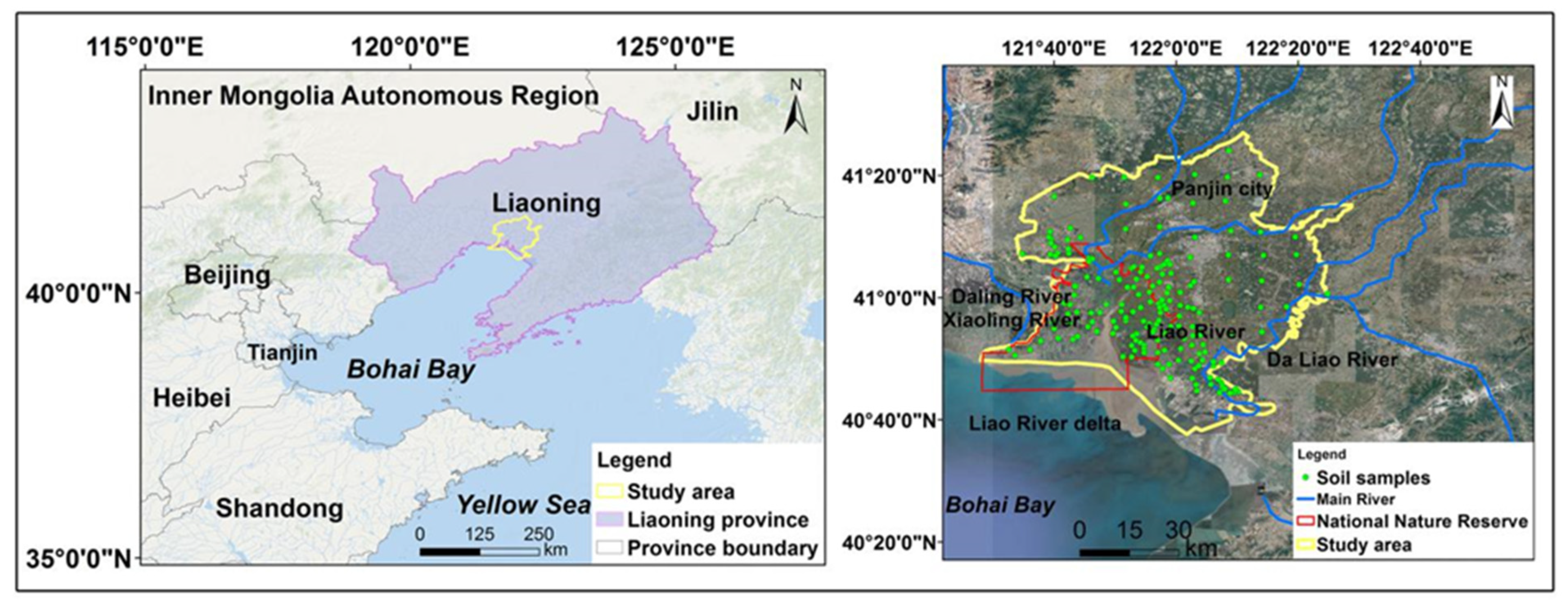
2.1. Study Area

Liao River delta (121°25′~122°31′E, 40°39′~41°27′N) belongs to the south of Liaoning Province, northeastern China. It is the estuary of the Liao River, Shuangtaizi River, Daling, and Xiaoling River. The administrative area of Panjin city was selected as the study area to integrate the socio-economic data, which covers the entire Liao River delta. Paddy fields, reed wetlands, and water areas are the main components of the region. The survey records revealed that there are many species migratory birds inhabiting and breeding in study area, 53% of the total species in China, mainly including red-crowned crane (Grus japonensis), and black-headed gull (Chroicocephalus saundersi) [42]. Agricultural activities are dominated by cultivation and aquaculture, industrial activities are dominated by oil exploitation, and built-up areas are dominated by roads or housing that have seriously damaged wetlands [42]. It has been recognized as in need of conservation with the designation of the Shuangtaizihekou (Liao River kou) national reserve in 1986, and the wetlands being listed as a Ramsar site since 2004 [41]. This reserve has been designated to strengthen the protection and management of wetland ecosystems.

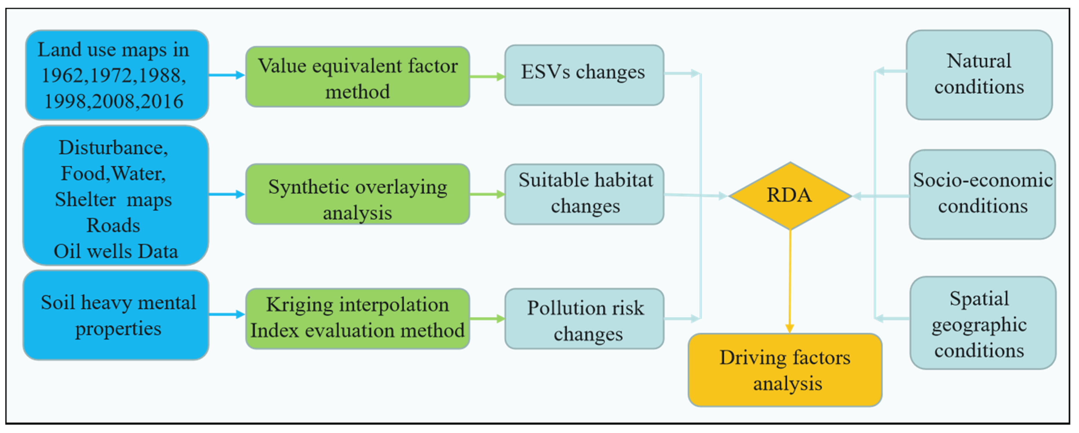
2.2. Data Collection and Process

The land use maps in 1988, 1998, 2008, and 2016 were interpreted based on Landsat TM/ETM images (https://earthexplorer.usgs.gov/). The land use maps in 1962 and 1972 were interpreted with Keyhole (KH5) (3.6 m × 3.6 m) and Keyhole (KH9) (0.3 m × 0.3 m) images (http://www.gscloud.cn/), including paddy field, dry farmland, built-up area, forestland, wetland, and water area, as seen in

Table 1. Characteristics of multi-year images and soil sample data used in the study.

Data	Date of Data	Description	Source
Land use map	25 August 1962	<3.6 m	Keyhole (KH5) https://earthexplorer.usgs.gov/
	2 May 1972	0.3 m	Keyhole (KH9) https://earthexplorer.usgs.gov/
	9 August 1988 14 May1998 20 October 2008 15 October 2016	30 m × 30 m	Landsat1,5,7,8 https://earthexplorer.usgs.gov/
184 Soil samples	October 2014	68 samples	National reserve
		116 samples	Out of national reserve

. A digital elevation model (DEM) (1:50,000) was collected from Liaoning surveying and Mapping Bureau. The images were pre-processed by registration, splicing, inlaid, and cutting for each year. The manual interpretation was used to get the classification results of land use. The annual normalized difference vegetation index (NDVI) from 1988 to 2016 was calculated using the maximum synthesis method (MVC) based on Google Earth Engine (https://earthengine.google.com/ for revision of the equivalent factors of ESVs). The spatial resolution of the data ranges from 0.3 m to 30 m, and all images were aggregated to 30 m spatial resolution by resampling. Taking the overall accuracy assessment to evaluate the accuracy of interpretations, 500 sample points were randomly selected in study area. The overall accuracy of the land use maps for 1962, 1972, 1988, 1998, 2008, and 2016 were 78.42%, 80.65%, 85.21%, 88.02%, 88.57%, and 89.35%, respectively. Manual interpretation and accuracy evaluation in 1962, 1972, and 1988 were mainly carried out by field surveys and historical records due to the smaller number of available data, which were affected by clouds, time, and other factors. The dataset of roads and oil wells was extracted from the above images. The social economic dataset, including population, GDP, agricultural and fishery output data, were collected based on the Panjin annual statistics book from 1962 to 2016, which were obtain from Liaoning statistical Bureau and field surveys.

A total of 184 soil samples (surface (0–5 cm) were selected in October 2014. The geographic positions of sampling sites were recorded using portable GPS units, which is distributed as shown in Figure 1. Three duplicates were extracted and mixed at each sampling site. Six soil heavy metal pollutants were tested, including cadmium (Cd), copper (Cu), chromium (Cr), nickel (Ni), zinc (Zn), and lead (Pb). The soil standard reference material (GBW07401, GSS-1) provided by the Center of National Standard Reference Material of China was used to control the test quality. Soil samples were treated with a microwave digestion instrument (CEM Inc., Matthews, NC, USA), and then tested for the concentrations of the heavy metals. The heavy metals were measured via inductively coupled plasma mass spectrometry (ICP-MS, PerkinElmer, Waltham, MA, USA) [43].

2.3. Land Use Dynamic Change Analysis Method

To quantitatively reflect the rate of land use change, the single dynamic index was used [44]. The land use TUPU analysis method was adopted to the land use change. The land use maps were used to build transfer matrix for information visualization of land use conversion. It was conducted to integrate the spatial information of the coded land use change value in ArcGIS. Specifically, the codes of the adjacent two phase maps were selected for the algebraic operation to obtain the value [20].

$$K=\frac{Ua-Ub}{Ua}\times \frac{1}{T}\times 100\%$$

(1)

where K represents the single dynamic index of land use, U_a and U_b represent the area of a certain land type at the beginning and the end of the period, respectively, and T represents the research period.

2.4. Comprehensive Evaluation Method

The comprehensive environmental effects were evaluated in this paper from three aspects, the change of ESVs, habitat suitability for water birds, and pollution risk of soil heavy mental. The ESVs and habitat suitability were assessed based on the value equivalent factor method and synthetic overlaying analysis of factors, respectively. The pollution risk was assessed by kriging interpolation and index evaluation. Then, the driving factors of comprehensive environmental effects were studied through redundancy analysis (RDA) from natural, socio-economic, and spatial geographic conditions, as shown in Figure 2.

2.4.1. Evaluation of the Ecosystem Service

The assessment method proposed by [29] has been widely calculated ESVs. The modification of the Chinese ecosystem coefficients was based on expert knowledge through over 700 ecologists [30,45], generating the table of the value per unit area of the ecosystem. The annual corrected equivalent factor was estimated at an equivalent ESVs of 410.80 US$/(hm² a) (based on the 2016 USD value; $1 could be converted to 6.67 RMB) based on the grain yield per unit area and the average grain price in 2016. The average equivalent ESVs coefficients of the wetlands were revised using the equivalent factors by the regional NDVI values, which may produce accurate results, especially in regions with large areas of reed wetland. Besides, built-up areas were not considered to provide ecosystem services [46]. Additionally, cultivated land was mentioned in this study, which includes paddy fields and dry farmland, for the ESVs calculation as following:

$$\begin{gathered} VCI=\left(\frac{NDVI-NDVImin}{NDVImax-NDVImin}\right)\times 100\% \\ ESV={\displaystyle \sum }_{j=1}^m{\displaystyle \sum }_{i=1}^n\left(LUAi\times VCij\right) \\ ESVcorrected=ESV\times \frac{VCIk}{\overline{VCI}} \end{gathered}$$

(2)

where $NDVI$, $NDVImax$, and $NDVImin$ indicate the annual average $NDVI$, the maximum, and minimum annual average $NDVI$ for the local grid, respectively. VCI indicates the vegetation condition index calculated from time-series NDVI. VCI is the annual average VCI in study area, $VCIk$ is the average $VCI$ in the k county. ESV and $ESVcorrected$ indicate the ecosystem service value before and after correction. $VCij$ indicates the $jth$ category of the coefficient for the $ith$ land use type, $LUAi$ indicates the $ith$ land use type area, n is the number of land use types, and m is the number of sub-categories of ESVs.

Sensitivity analysis was calculated the coefficient of sensitivity of the value coefficient, to test whether the results of the ESV coefficient are credible. This method was used to modify the value coefficient of each land use type by (±) 50%, and then the changes of corresponding ESVs were calculated. The reliability of the ESVs results can be verified by sensitivity analysis [24], and the index can be calculated as:

$$CS=\left|\frac{\left(ESVj-ESVi\right)/ESVi}{\left(VCjk-VCik\right)/VCik}\right|$$

(3)

where CS represents the coefficient of sensitivity. When CS < 1, it indicates that ESV lacks flexibility for VC, and the resulting reliability is high, When CS > 1, just the opposite. $ESVi$ and $ESVj$ indicate the ESVs before and after the adjustment, $VCi$ and $VCj$ indicate the ESV coefficients before and after the adjustment, and k represents the land use type.

2.4.2. Evaluation of Suitable Habitat for Birds

Estuarine wetlands in the Liao River delta are crucial bird migration stopover sites. A combination of single factor extraction and the merging method was used to establish the suitable habitat for birds [33]. In order to obtain scientific evaluation results, field surveys combined with consulting experts were used to select and determine six factors that affected the bird habitat, namely disturbance degree, food richness, water condition, shelter condition, roads, and oil wells. The classification of disturbance degree, food richness, and water condition were based on the land use classification, and NDVI analysis for shelter condition was also required. Based on previous research results and the field surveys, the characteristics of suitable habitat for birds was determined [47]. Taking the red-crowned crane, which is highly sensitive to disturbance, the nearest distance to a road needs to be 410 m, and to an oil well is 500 m [48]. These six types of habitat factor maps were carried out by synthetic overlaying analysis, which is used to combine and overlay among factor maps in spatial analysis, and generated suitable habitat maps to reflect the bird habitat changes.

2.4.3. Pollution Risk Assessment

The geo-accumulation index was used to assess the soil heavy metal contamination level [49]. The potential ecological risk index (RI) was evaluated the level of heavy metal pollution in topsoil, indicating the toxicity and environmental response of the soil heavy metals [50]. The kriging interpolation method was adopted to calculate the spatial distribution of the pollution. The equations are as follows:

$$\begin{gathered} \mathrm{Igeo}=\frac{Ci}{1.5\times Bi} \\ RI={\displaystyle \sum _{\mathrm{i}=1}^{\mathrm{m}}{{\displaystyle E}}_r^i}={\displaystyle \sum _{i=1}^m{{\displaystyle T}}_r^i}\times {{\displaystyle C}}_j^i={\displaystyle \sum _{i=1}^m{{\displaystyle T}}_r^i}\times \frac{{{\displaystyle c}}_0^i}{{{\displaystyle c}}_n^i} \end{gathered}$$

(4)

where $\mathrm{Igeo}$ is the geo-accumulation index of a sampling point, C_i represents heavy metal i concentration in topsoil, B_i is the background value of heavy metal i [51], which is obtained from Chinese soil element background value, and 1.5 is the background matrix correction factor. $E_r^i$ is the single potential ecological risk factor, $T_r^i$ is the toxic-response factor for a given substance, which accounts for the toxic requirement and the sensitivity requirement, and RI represents the sum of all risk factors, as shown in

Table 2. Description of the $\mathrm{Igeo}$, risk factor ($E_r^i$), and risk index (RI) ranks as suggested by [43].

Igeo	${\mathit{E}}_{\mathit{r}}^{\mathit{i}}$	RI	Ecological Risk Ranks
<1	<40	<70	low
1–2	40–80	70–140	moderate
2–3	80–160	140–280	considerable
3–5	160–320	-	high
>5	≥320	≥280	very high

. $C_j^i$ represents the contamination factor, $C_0^i$ and $C_n^i$ are the concentration and a reference value for soil heavy metal, respectively. In this paper, the soil background values of Liaoning province were considered as references to evaluate the present pollution conditions and the potential for ecological impacts.

2.4.4. Driving Factors Analysis

The redundancy analysis (RDA) was applied to analyze the relationship between the wetland loss and the environmental effects. The determination of factors was chosen based on related studies [17,52]. A total of 13 factors from 3 aspects were chosen. Four variables were selected to represent socio-economic conditions, including population, GDP, agricultural, and fishery output. The five variables reflected the natural conditions, including the NDVI, soil texture, wetland area, agriculture area, and soil heavy metal contamination. Four variables were selected to represent the spatial geographic conditions, including the distance to a river, distance to a road, distance to a city, and distance to an oil well. The ESVs, suitable habitat area, and RI were selected to represent ecological services, suitable habitat, and soil heavy metal potential risk. A detrended correspondence analysis (DCA) was proceed to choose the most valid ordination method. The RDA method was chosen due to the gradient length was less than 3 (0.3). According to the values of contribution and significance, the major factors that affected the dependent variables were selected by the interactive forward-selection method. The RDA method was performed by the selected factors, which was undertaken based on the software CANOCO 4.5 [53].

3. Results

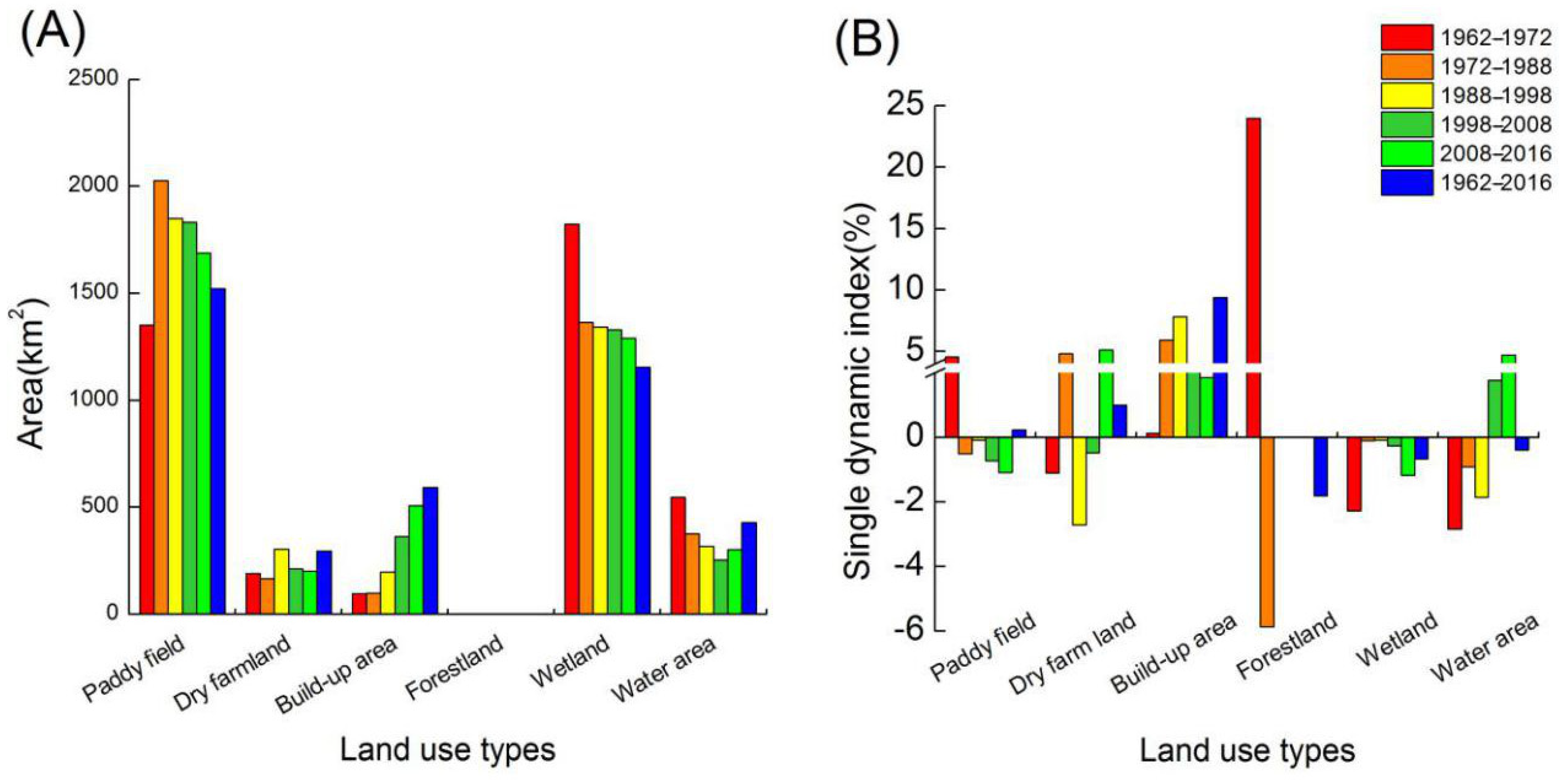
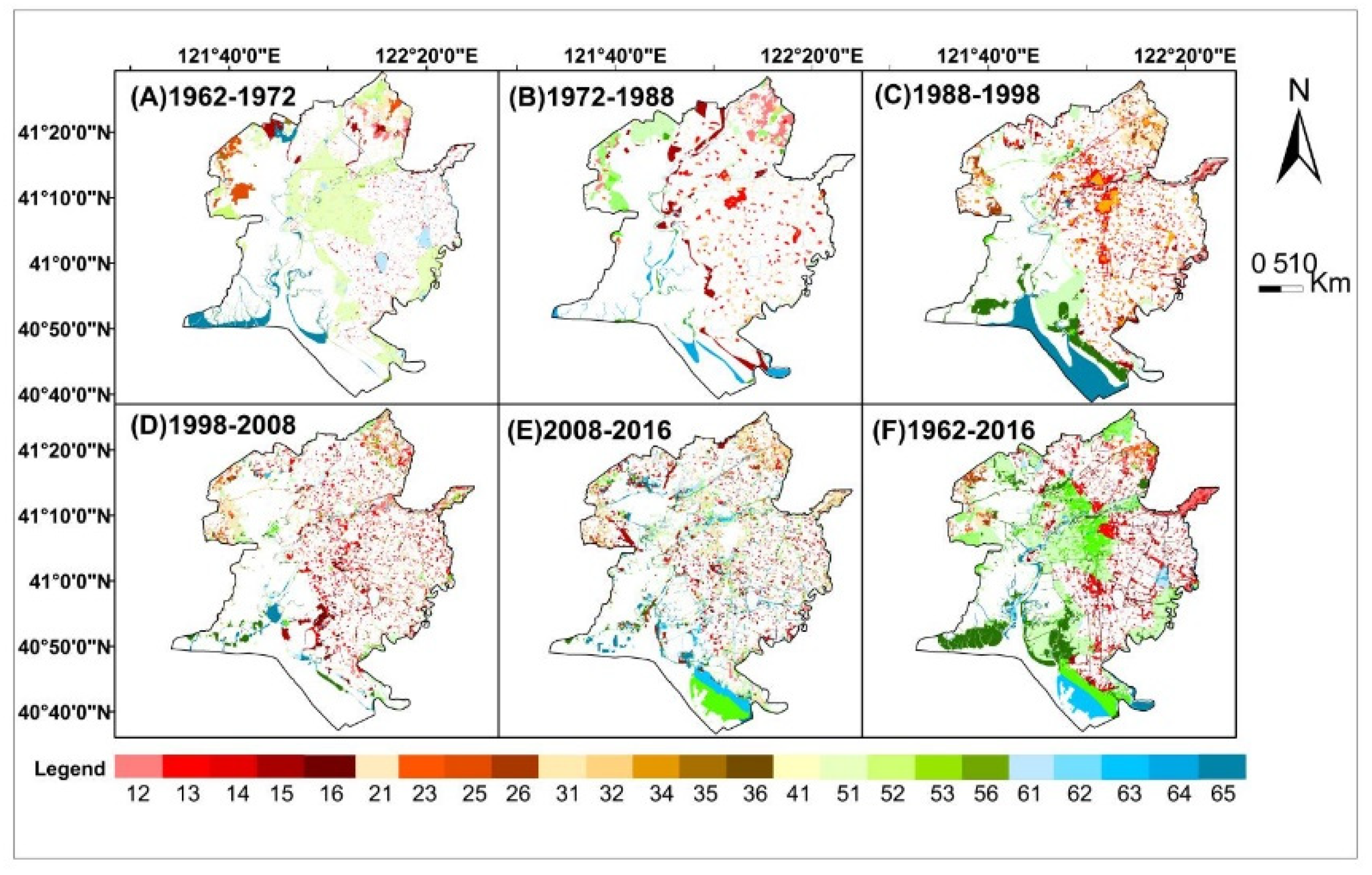
3.1. Spatial and Temporal Changes in Land Use

The area of paddy fields, dry farmland, wetland, forestland, built-up areas, and water area were 1351.30 km², 189.5 km², 1823.16 km², 0.2 km², 95.98 km², and 546.22 km², respectively, in 1962. By 2016, the areas were 1522.39 km², 294.14 km², 591.49 km², 0 km², 1153.52 km², and 428.96 km², respectively. Wetland and water area decreased 669.64 and 117.26 km², and built-up areas, paddy fields, and dry farmland increased by 495.51, 171.08, and 104.65 km² during 1962–2016, respectively. A single dynamic index (Figure 3) showed that the built-up area had a continuous increase (0.13%, 5.92%, 7.82%, 3.59%, and 1.86%), and the change rate of built-up areas peaked from 1988 to 1998. Conversely, a continuous declining tendency (2.85%, 0.10%, 0.09%, 0.26%, and 1.18%) was observed in wetlands, and the wetland loss was the fastest in the first and the last periods. Forestland rarely appeared since the 1980s. The water area was gradually decreasing before the 1990s, and then, the water area remarkably increased to a proportion of 4.72% during 2008–2016.

The characteristics of land use in spatial distribution exhibited significant differences during 1962–2016 (Figure 4). The wetlands were converted to paddy fields (25.30%), dry farmland (5.96%), built-up areas (13.15%), and water areas (16.43%). The conversion of “wetland-paddy field” (Figure 4 code 51) had the largest change in area of 471.79 km², which indicated that the wetland was being cultivated. Meanwhile, the conversion of “wetland-water area” (Figure 4 code 56) for 306.28 km² and “wetland-built-up area” (Figure 4 code 53) for 245.19 km² took the second and third change area order, which reflected that the wetland was mainly being occupied by aquaculture activities, urban expansion, and harbor construction. The water area was converted to built-up areas (Figure 4 code 56) of 88.06 km², which were distributed along the Liao River and coastal zone. The paddy fields, dry farmland, and water area were converted to built-up areas with proportions of 9.13%, 2.00%, and 4.73%, respectively. The “land use change” was slight at the core of the delta since 1988, which is mostly distributed in natural reserves, indicating that wetland resources were effectively protected in the Liao River delta through establishment of the reserve.

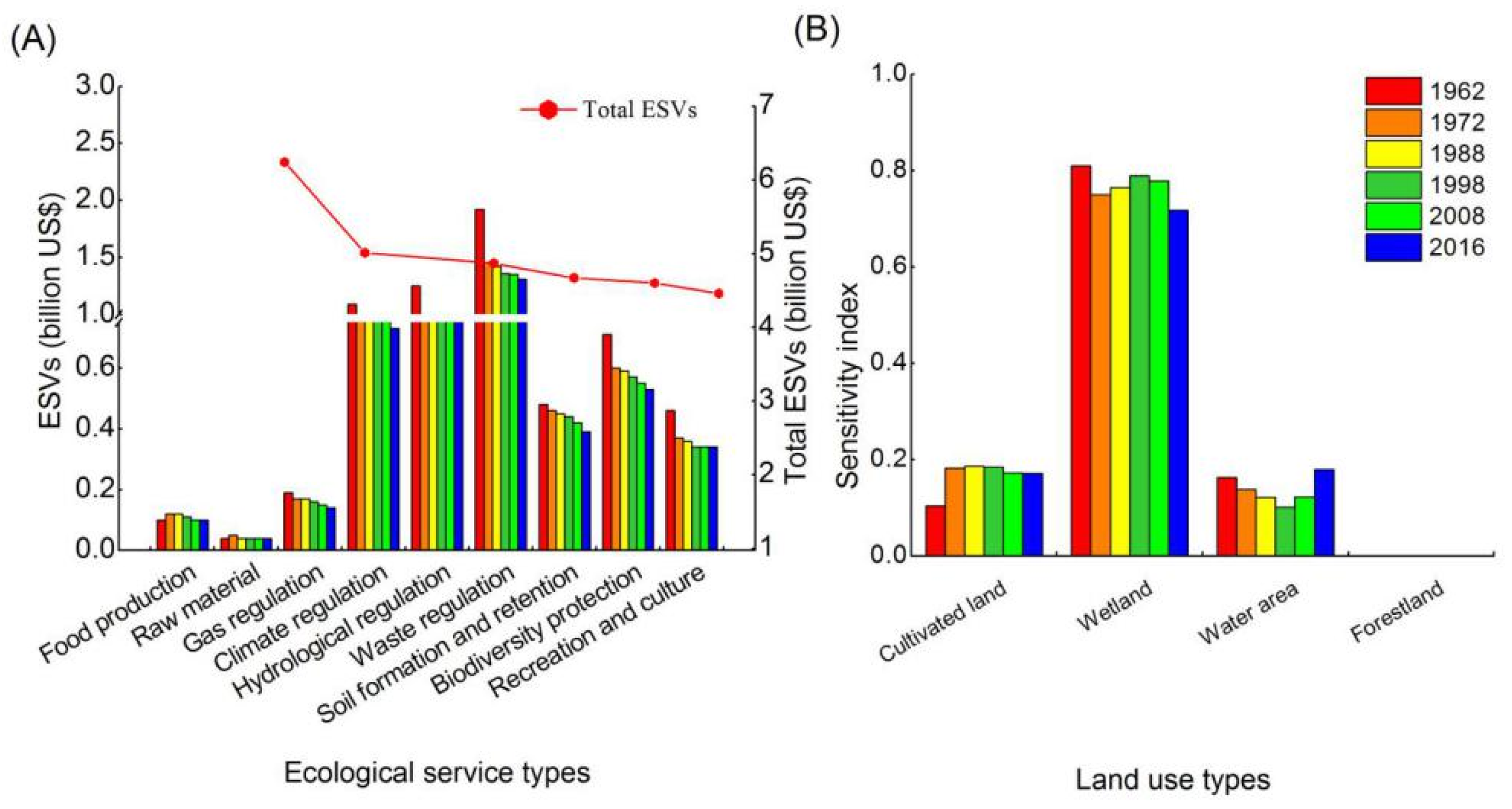
3.2. Ecosystem Services Changes

The ESVs results were 6.24, 5.01, 4.87, 4.67, 4.60, and 4.46 billion US$ in 1962, 1972, 1988, 1998, 2008, and 2016, respectively. The ESVs had lost about 1.78 billion US$, accounting for 28.58% since 1962 (

Table 3. Change in ecosystem service values (ESVs) from 1962 to 2016 in Liao River delta.

Categories	Sub-Categorie/Billion Dollars	1962	1972	1988	1998	2008	2016	1962–2016(%)
Supplying services	Food production	0.10	0.12	0.12	0.11	0.10	0.10	−1.11
	Raw material	0.04	0.05	0.04	0.04	0.04	0.04	0.33
Regulating services	Gas regulation	0.19	0.17	0.17	0.16	0.15	0.14	−22.50
	Climate regulation	1.09	0.85	0.84	0.82	0.80	0.73	−33.01
	Hydrological regulation	1.25	0.93	0.88	0.82	0.84	0.88	−29.43
	Waste regulation	1.92	1.46	1.42	1.36	1.35	1.31	−31.58
Supporting services	Soil formation and retention	0.48	0.46	0.45	0.44	0.42	0.39	−20.47
	Biodiversity protection	0.71	0.60	0.59	0.57	0.55	0.53	−26.00
Cultural services	Recreation and culture	0.46	0.37	0.36	0.34	0.34	0.34	−26.89
	Total	6.24	5.01	4.87	4.67	4.60	4.46	−28.58

). The values of waste regulation and hydrological regulation were the highest ones, followed by climate regulation, biodiversity protection, soil formation and retention, recreation and culture, gas regulation, and raw material production (Figure 5A). The ESVs values of ecological service functions showed a declining change, however the ESVs of raw material had an increasing trend (0.33%) from 1962 to 2016. The declining ESVs were mainly caused by the loss of wetland, which has the highest ecological services. Additionally, forestland and water areas were converted to cultivated land, which led to an increase in raw materials. The values of regulating services decreased (22.50%, 33.01%, 29.43%, and 31.58%), and the values of supporting services decreased (20.47% and 26.00%) 1962–2016. Regulating services and supporting services were contributed to the ESVs with the large proportion that were observed. The ESVs of wetland and water area decreased significantly, with the proportions of 36.73% and 21.47%, and the ESVs of cultivated land increased 17.89% (

Table 4. ESVs change rate (%) of each land use type from 1962 to 2016.

Type	Year	Cultivated Land	Wetland	Water area	Forestland
Change rate (%)	1962–1972	42.33	−25.13	−31.34	292.50
	1972–1988	−1.77	−1.62	−15.47	−100.00
	1988–1998	−5.05	−1.04	−20.45	--
	1998–2008	−7.63	−2.88	19.39	--
	2008–2016	−3.86	−10.62	42.46	--
	1962–2016	17.89	−36.73	−21.47	--

). The wetland contributes the most to the ESVs, followed by cultivated land and water area. Compared with other land use types, the ESVs of wetland always showed negative changes during 1962–2016. The area with high ESVs has gradually decreased, and the area with low ESVs has increased 1962–2016.

The results of ESVs were not flexible relative to the value coefficient due to the CS value was less than 1. The CS values in descending order were wetland > cultivated land > water area > forestland (Figure 5B). The CS value of wetland in 1962 was the highest, up to 0.8, which shows a higher decreasing trend than the other land use types. Moreover, the CS values of cultivated land and water area had relatively large effects on the total ESVs. The results of ESVs were not flexible to the VC value, which was observed by sensitivity analysis, and even though the VC value was uncertain, the results were still stable.

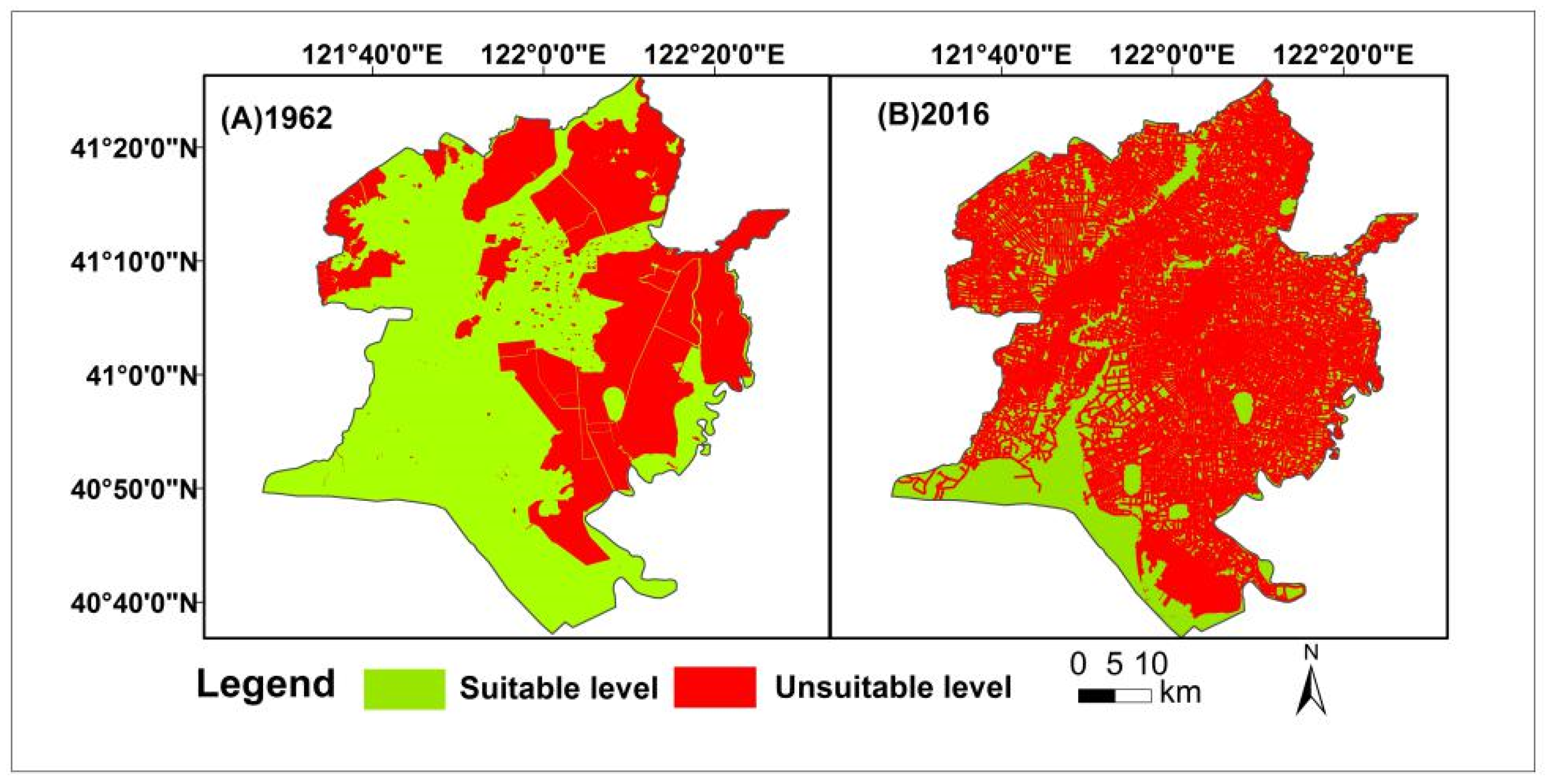
3.3. Birds Suitable Habitat Changes

The suitable habitat for birds was divided into the suitable and unsuitable habitat. The results showed that the suitable habitat was constantly decreasing with a degradation trend (Figure 6). The area of bird suitable habitat declined from 2359.80 km² in 1962 to 910.31 km² in 2016 due to the wetlands being cultivated and the urbanization process, which experienced a continuous decrease of 1449.49 km², with a proportion of 61.42%. The wetland was dominated by natural wetland, such as reed swamp with rare built-up areas, obviously without oil wells. The bird habitat area accounted for 59% of the study area in 1962. Suitable habitat for birds was mainly distributed in the estuarine wetlands in 2016, which reflects that the wetland and tidal-flats in the Liao River delta are the main habitats of birds. Contrarily, the unsuitable habitat area was gradually increasing, mainly distributed around built-up areas and oil wells.

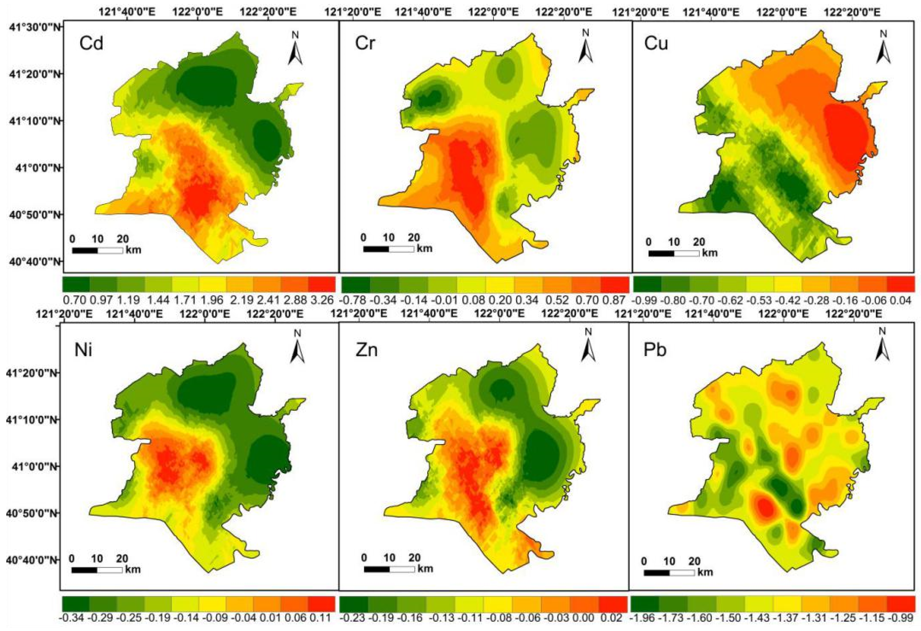
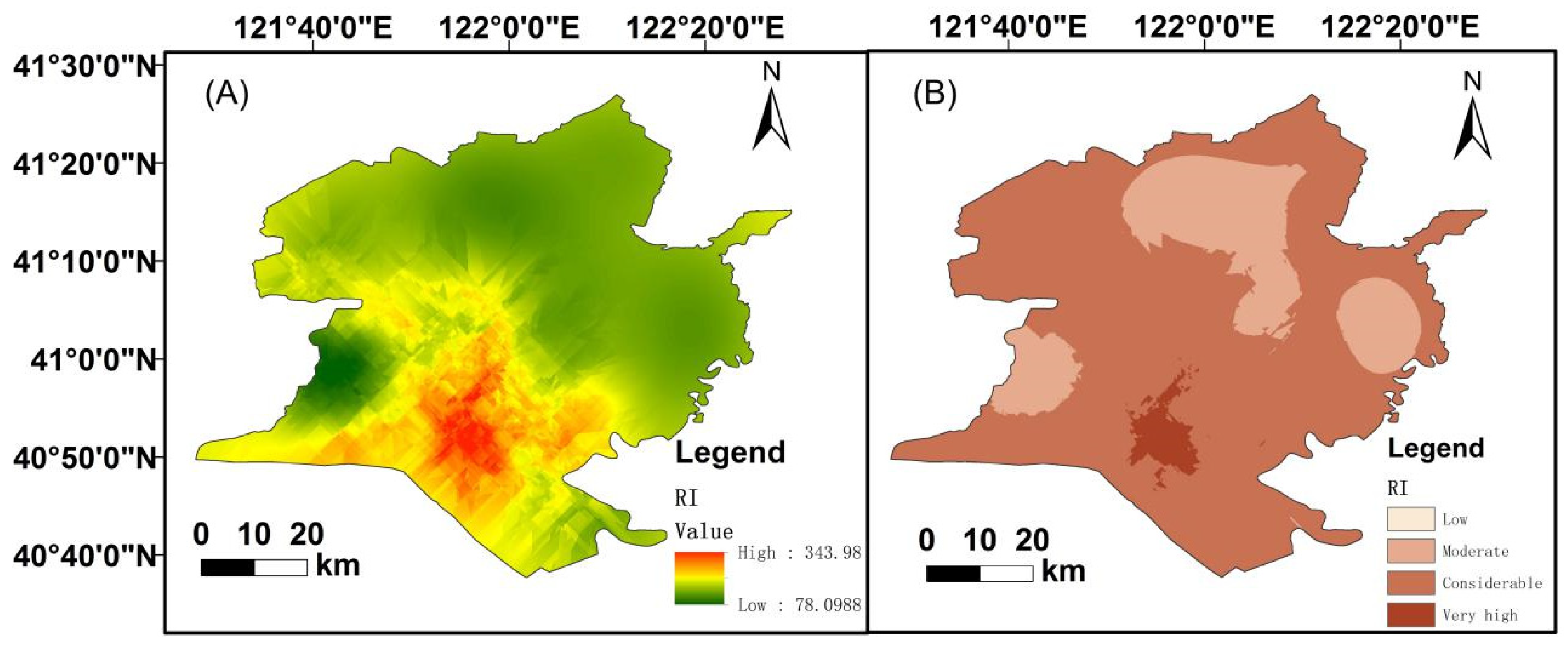
3.4. Potential Soil Pollution Ecological Risk

The statistical results indicated that the mean concentrations of soil heavy metals were measured, Cr (154.95 ± 52.16), Zn (102.21 ± 19.44), Ni (40.71 ± 9.13), Cu (17.23 ± 6.05), Pb (11.97 ± 3.66), and Cd (1.41 ± 0.82) (

Table 5. Summary statistics of heavy metal concentrations and properties in the topsoil [51].

	Minimum	Maximum	Average	S.D.	CV(%)	Background Value (China)	Background Value (Liaoning Province)
Cu(mg/kg)	4.55	31.67	17.23	6.05	35.1	22.6	19.8
Cr (mg/kg)	50.65	275.79	154.95	52.16	33.66	61	57.9
Cd (mg/kg)	0.26	3.46	1.41	0.82	58.23	0.097	0.108
Ni (mg/kg)	20.87	59.34	40.71	9.13	22.44	26.9	25.6
Zn (mg/kg)	53.4	149.5	102.21	19.44	19.02	74.2	63.5
Pb (mg/kg)	2.95	19.57	11.97	3.66	30.54	26	21.4

). The coefficient of variation of heavy metals was within the range of 12.65–58.23%. Particularly, the concentrations of Cd, Cr, Cu, and Pb had a high coefficient of variation (>30%), which indicated that soil heavy metals have similar sources. The Ni and Zn had a low coefficient of variation (<30%), which indicated they were more uniformly distributed in the study area. Among them, the mean concentrations of Cd, Cr, Ni, and Zn were all above the local soil background values.

The ${\mathrm{I}}_{\mathrm{geo}}$ values and ranks of pollutants at each sampling point are presented in Figure 7. The ${\mathrm{I}}_{\mathrm{geo}}$ values of Cd ranged from 0.70–3.26, with the highest value in paddy fields and the lowest value in built-up areas. Cd reached a high level. The ${\mathrm{I}}_{\mathrm{geo}}$ values of Cr reached light to moderate levels. Cr with highest ${\mathrm{I}}_{\mathrm{geo}}$ value was around the core of the Liao River estuary. The pollution hotspots of Zn were closer to the paddy fields, wetlands, and built-up areas, which reached a moderate level. Some Ni pollution hot spots were found near oil wells in the wetlands. The ${\mathrm{I}}_{\mathrm{geo}}$ values of Cu and Pb were almost 0, revealing that their level of pollution is relatively low. The ${\mathrm{I}}_{\mathrm{geo}}$ values were ranked as Cd > Cr > Ni > Cu > Zn > Pb.

The Cd posed a considerable potential ecological risk at 184 sampling points. The high ecological risks of Cd are the consequences of fertilizers and pesticides used in agriculture activities. Ni posed the second largest ecological risk. For Cu, Cr, Zn, and Pb, the risk indexes were low levels. $E_r^i$ indicated that the degree of pollution of the soil heavy metals decreased as follows: Cd > Ni > Cu > Cr > Pb > Zn. The mean value of RI was 343.98, which indicated that all sample sites arrived at a moderate potential ecological risk level in Figure 8A. A total of 81 of 184 sites exhibited considerable or high ecological risk. The RI values were significantly correlated with the presence of oil wells. The RI of estuarine wetlands in the reserve were at low and moderate levels as shown in Figure 8B. The distributions of Cd and the RI were similar, indicating that the RI was impacted by Cd.

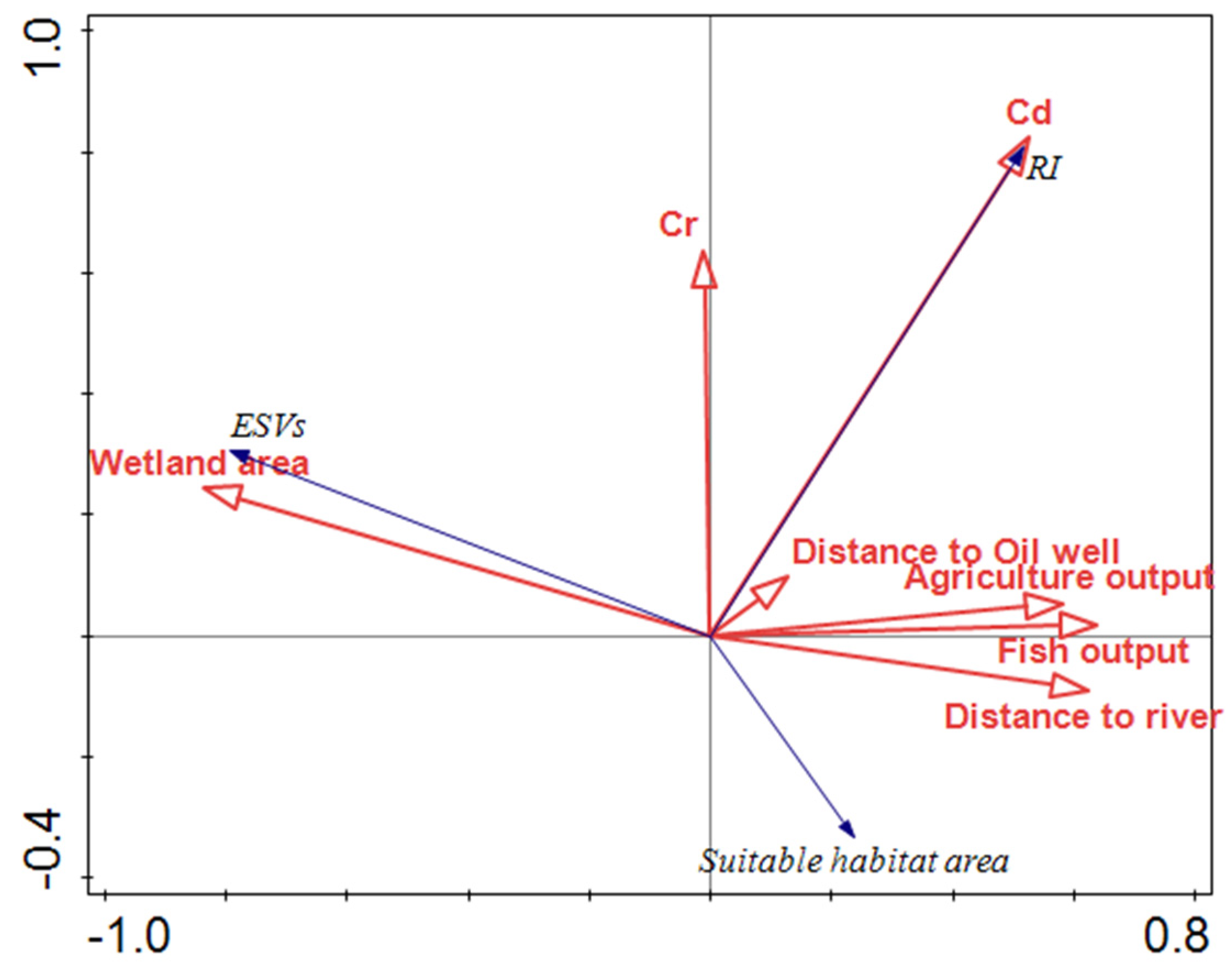
3.5. Relationships among the Changes of Ecological Effects and Factors

The results showed that the wetland area, Cd concentrations, Cr concentrations, distance to oil wells, distance to a river, and agricultural and fishery output have power in explaining the ESV, RI, and suitable habitat (p < 0.05). Approximately 74.70% of the variation were explained by the selected variables. The first two ordination axes explained over 78.0% of the correlation with both the driving factors of wetland loss and ecological effects (p = 0.01). The results indicated that the percentage of wetland area had a greater impact on environmental effects, with contributions of 44.5%, and the Cd concentrations also had a greater impact, with contributions of 37.3% in

Table 6. Selected variables for further redundancy analysis (RDA) by the Monte Carlo permutation test (n = 499).

Variables	Explanation (%)	Contribution (%)	Pseudo-F	Significance-p
Wetland area	36.0	44.5	23.1	0.002
Cd	30.2	37.3	35.9	0.002
Distance to river	5.7	7.6	8.0	0.012
Fishery output	3.2	3.9	4.9	0.024
Cr	1.8	2.2	2.9	0.049
Agricultural output	1.5	1.8	2.5	0.048
Distance to oil wells	0.5	0.6	0.8	0.040

. As shown in Figure 9, RI was positively related to Cd, Cr, agriculture and fishery output, and the distance to oil wells and negatively related to the wetland area. Wetland area has a negative relationship with the potential ecological risk. A positive correlation between wetland area and ESVs was found, which demonstrated that the change of wetland is likely to lead to ESV loss. Suitable habitat area was positively related to the distance to rivers, and negatively related to the distance to an oil well, which indicated that the water condition is an important factor for bird habitats and oil exploration is likely to lead to suitable habitat loss. The wetland loss and driving factors, such as agriculture, oil wells, and industrial exploitation have resulted in cumulative environmental effects.

4. Discussion

4.1. Influence Process of Wetland Loss on Ecological Effects

The wetland was the primary land use type in the Liao River delta during 1962–2016. However, the wetland area has decreased dramatically, mainly being converted into cultivated land and built-up areas. The wetland has been developed as farmland, built-up areas, and aquaculture in the past few decades [54]. Some surveys were carried out on the changes of wetlands, such as the Yellow River delta, Yangtze River delta, Sanjiang plain, and Jiangsu coastal zone. Comparing the wetlands loss in the Liao River delta to those four areas showed that wetland loss was common. For example, the coastal wetland in Jiangsu has lost about 323.46 km² over the past 10 years [55], and wetland loss in Sanjiang plain has reached 73.3% (about 27,700 km²) since 1954 [56]. The ESVs lost in the Yellow River delta has decreased by about 10.89% in 2009–2015 [57], and the ESVs of Yangtze River delta has lost about 2.12 billion US$ 2009–2016 [58]. A continuous declining tendency was observed in ESVs of wetlands due to wetland being converted to cultivated land, since the ESVs of cultivated land increase significantly [56]. Conversion of wetland to agricultural land increases the material production values, however the conversion led to the ESVs loss of wetlands for pollution purification, biodiversity conservation, leisure and entertainment. In particular, this is critical to migratory birds since in the Liao River delta, suitable habitat for birds has lost from 135.77 to 74.24 km² along the Yangtze River 1986–2015 [59]. The suitable habitat for birds is constantly decreasing with a degradation trend in the study area, due to dam construction raised the terrain and silted up the sediment, resulting in the lack of water. Aquaculture has led to the degradation or even disappearance of wetland plant communities, which means the birds have no shelter. Potential ecological risk of heavy metal in the Yellow River delta and the Yangtze River delta are at a high level for Cd [60,61]. The comparison indicated that Cd was the primary pollutant at a high pollution level in the coastal and estuarine areas. Scholars have revealed that Pb pollution is largely related to the exploitation of mines [43]. Some Pb pollution hotspots are more evenly distributed around roads in the study area. The atmospheric Pb caused by the burning of gasoline may be the reason for the distribution of its pollution hot spots. Analysis of all these factors involved in eco-environmental changes have rarely been integrated in the past, but they are comprehensively analyzed and studied in this paper.

4.2. Policy Implications

Ecological effects always affect the human well-being and sustainable developments. The conservation of ecosystem and economic development are emphasized in national decision-making reports. Historically, the delta was a swamp area with a small human population. Agriculture and aquaculture developed rapidly after reclamation departments were established in 1960s. After oil and gas were discovered, oil production activities began in 1970. The region has experienced rapid economic growth based on the overexploitation of resources and agriculture activities, which has caused a series of environmental problems. The establishment of a national reserve and the implementation of wetland restoration projects [62], such as “returning cultivated land to wetland”, has restored tidal flats and marshes, and the facilities that threaten ecosystems have been reduced. In order to achieve the coordinated development of ecological, economic, and social benefits, the ‘‘three lines” (three lines—Permanent basic farmland red line, Urban development boundary, and Ecological red line) should be promoted in China [20,63]. The “Ecological Red Line” policy formed the boundary lines of the key ecological protection area and has important strategic value for ecological security and sustainable development in the Liao River delta. Wetland protection is the prerequisite for development and utilization, so where is the red line of development? The ecological red line of wetland ecosystem is supported in the implementation of controls, which guides the economical and intensive use of wetland resources for sustainable development. The combination of the ecological red line and land use transition to build a regional ecological security pattern can better strengthen regional ecological protection and curb the degradation of the ecosystem. The results of this paper can be regarded as a reference in policy decision-making.

4.3. Validity and Limitations

The wetland changes and its ecological effects were studied in this study. The wetland ecosystem is an essential part of the Liao River delta. Which factors have the greatest impact on wetland changes? The dominant factor is still controversial due to many factors driving wetland changes [13]. Many studies have indicated that natural and socio-economic factors mainly lead to the wetland changes [7,52]. A total of 13 representative factors were chosen for analysis, and we also considered spatial geographic conditions in this study. Besides, the ESVs were calculated with modified coefficients. The price of production was decided by the mean values in Panjin city in 2016 in this study. The grain yield per unit area was selected as the revised index by related literatures [30], and the coverage coefficient was selected according to the correlation between the NDVI and the ESVs. Due to the obvious seasonal differences, NDVI data should be chosen to match the time of the study. Moreover, it is revised from the scale of nation to region, in order to ensure the comparability of the equivalents under different scales and to show the heterogeneity of the ESVs in spatial distribution. The NDVI data of 1962 and 1972 were not obtained, and the grain yield per unit area has not been revised by the coefficient. A sensitivity index was used to verify the results of the ESVs, and proved to be reliable. Applying comprehensive and explanatory evaluations such as those employed here will be key to future conservation of wetland resources in estuarine areas.

5. Conclusions

This paper analyzed the main land use type changes in the Liao River delta during 1962–2016, and estimated the changes of ESVs, the suitable habitat, and risk assessment of soil heavy metals. We have reached the following conclusion. The area of wetland has decreased 669.64 km², with a proportion of 36.73%. The “wetland-paddy field” is the major change. The ESVs has lost about 1.78 billion US$ in 1962–2016. Regulating services and supporting services mainly contributed to the total ESVs. The suitable habitat area was decreased by 1449.49 km², with a proportion of 61.42%. Cd pollution is the highest soil pollution ecological risk in the Liao River delta, followed by Ni, Cu, Cr, Pb, and Zn. Wetland area, Cd, Cr, distance to a river, distance to an oil well, and agricultural and fishery output also had impacts on ecological environmental effects. This paper put forward a set of methods to evaluate the environmental changes of estuarine wetland ecosystem. The implications of this paper provide some references for wetland conservation and the sustainable development of the region, as well as other estuaries area.

References

1. Junk, W.J.; An, S.; Finlayson, C.M.; Gopal, B.; Květ, J.; Mitchell, S.A.; Mitsch, W.J.; Robarts, R.D. Current state of knowledge regarding the world’s wetlands and their future under global climate change: A synthesis. Aquat. Sci. 2013, 75, 151–167. [Google Scholar] [CrossRef] [Green Version]
2. García, J.; Solimeno, A.; Zhang, L.; Marois, D.; Mitsch, W.J. Constructed wetlands to solve agricultural drainage pollution in South Florida: Development of an advanced simulation tool for design optimization. J. Clean. Prod. 2020, 258, 120868. [Google Scholar] [CrossRef]
3. Gardner, R.C.; Barchiesi, S.; Beltrame, C.; Finlayson, C.M.; Galewski, T.; Harrison, I.; Paganini, M.; Perennou, C.; Pritchard, D.E.; Rosenqvist, A.; et al. State of the World’s Wetlands and Their Services to People: A Compilation of Recent Analyses. Ramsar Briefing Note No. 7; Ramsar Convention Secretariat: Gland, Switzerland, 2015. [Google Scholar]
4. Debanshi, S.; Pal, S. Modelling water richness and habitat suitability of the wetlands and measuring their spatial linkages in mature Ganges delta of India. J. Environ. Manag. 2020, 271, 110956. [Google Scholar] [CrossRef] [PubMed]
5. Thorslund, J.; Jarsjo, J.; Jaramillo, F.; Jawitz, J.W.; Manzoni, S.; Basu, N.B.; Chalov, S.R.; Cohen, M.J.; Creed, I.F.; Goldenberg, R.; et al. Wetlands as large-scale nature-based solutions: Status and challenges for research, engineering and management. Ecol. Eng. 2017, 108, 489–497. [Google Scholar] [CrossRef]
6. Zhou, J.; Wu, J.; Gong, Y. Valuing wetland ecosystem services based on benefit transfer: A meta-analysis of China wetland studies. J. Clean. Prod. 2020, 276, 122988. [Google Scholar] [CrossRef]
7. Lu, Q.; Bai, J.; Zhang, G.; Wu, J. Effects of coastal reclamation history on heavy metal in different wetland type soils in the Pearl River Delta: Levels, sources and ecological risks. J. Clean. Prod. 2020, 272, 122668. [Google Scholar] [CrossRef]
8. Huang, Y.; Sun, W.J.; Zhang, W.; Yu, Y.Q.; Su, Y.H.; Song, C.C. Marshland conversion to cropland in northeast China from 1950 to 2000 reduced the greenhouse effect. Glob. Chang. Biol. 2010, 16, 680–695. [Google Scholar] [CrossRef]
9. Pendleton, L.; Donato, D.C.; Murray, B.C.; Crooks, S.; Jenkins, W.A.; Sifleet, S.; Craft, C.; Fourqurean, J.W.; Kauffman, J.B.; Marba, N.; et al. Estimating global “blue carbon” emissions from conversion and degradation of vegetated coastal ecosystems. PLoS ONE 2012, 7, e43542. [Google Scholar] [CrossRef] [Green Version]
10. Tian, W.; Qiao, K.; Yu, H.; Bai, J.; Jin, X.; Liu, Q.; Zhao, J. Remediation of aquaculture water in the estuarine wetlands using coal cinder-zeolite balls/reed wetland combination strategy. J. Environ. Manag. 2016, 181, 261–268. [Google Scholar] [CrossRef]
11. Mulder, J.P.M.; Hommes, S.; Horstman, E.M. Implementation of coastal erosion management in the Netherlands. Ocean Coast. Manag. 2011, 54, 888–897. [Google Scholar] [CrossRef]
12. Gedan, K.B.; Silliman, B.R.; Bertness, M.D. Centuries of human-driven change in salt marsh ecosystems. Annu. Rev. Mar. Sci. 2009, 1, 117–141. [Google Scholar] [CrossRef] [PubMed] [Green Version]
13. Velez, J.M.M.; Garcia, S.B.; Tenorio, A.E. Policies in coastal wetlands: Key challenges. Environ. Sci. Policy 2018, 88, 72–82. [Google Scholar] [CrossRef]
14. Davidson, N.C. How much wetland has the world lost? Long-term and recent trends in global wetland area. Mar. Freshw. Res. 2014, 65, 934–941. [Google Scholar] [CrossRef]
15. Alam, M. Ecological and economic indicators for measuring erosion control services provided by ecosystems. Ecol. Ind. 2018, 95, 695–701. [Google Scholar] [CrossRef]
16. Lawler, J.J.; Lewis, D.J.; Nelson, E.; Plantinga, A.J.; Polasky, S.; Withey, J.C.; Helmers, D.P.; Martinuzzi, S.; Pennington, D.; Radeloff, V.C. Projected land-use change impacts on ecosystem services in the United States. Proc. Natl. Acad. Sci. USA 2014, 111, 7492–7497. [Google Scholar] [CrossRef] [PubMed] [Green Version]
17. Sica, Y.V.; Quintana, R.D.; Radeloff, V.C.; Gavier-Pizarro, G.I. Wetland loss due to land use change in the Lower Parana River Delta, Argentina. Sci. Total Environ. 2016, 568, 967–978. [Google Scholar] [CrossRef]
18. Chuai, X.W.; Huang, X.J.; Wu, C.Y.; Li, J.B.; Lu, Q.L.; Qi, X.X.; Zhang, M.; Zuo, T.H.; Lu, J.Y. Land use and ecosystems services value changes and ecological land management in coastal Jiangsu, China. Habitat Int. 2016, 57, 164–174. [Google Scholar] [CrossRef]
19. Wang, S.L.; Xu, X.R.; Sun, Y.X.; Liu, J.L.; Li, H.B. Heavy metal pollution in coastal areas of South China: A review. Mar. Pollut. Bull. 2013, 76, 7–15. [Google Scholar] [CrossRef]
20. Chen, W.; Zhao, H.; Li, J.; Zhu, L.; Wang, Z.; Zeng, J. Land use transitions and the associated impacts on ecosystem services in the Middle Reaches of the Yangtze River Economic Belt in China based on the geo-informatic Tupu method. Sci. Total Environ. 2020, 701, 134690. [Google Scholar] [CrossRef]
21. Owethu Pantshwa, A.; Buschke, F.T. Ecosystem services and ecological degradation of communal wetlands in a South African biodiversity hotspot. R. Soc. Open Sci. 2019, 6, 181770. [Google Scholar] [CrossRef] [Green Version]
22. Gu, J.; Luo, M.; Zhang, X.; Christakos, G.; Agusti, S.; Duarte, C.M.; Wu, J. Losses of salt marsh in China: Trends, threats and management. Estuar. Coast. Shelf Sci. 2018, 214, 98–109. [Google Scholar] [CrossRef] [Green Version]
23. Westman, W.E. How much are nature’s services worth? Science 1977, 197, 960–964. [Google Scholar] [CrossRef] [PubMed]
24. Kreuter, U.P.; Harris, H.G.; Matlock, M.D.; Lacey, R.E. Change in ecosystem service values in the San Antonio area, Texas. Ecol. Econ. 2001, 39, 333–346. [Google Scholar] [CrossRef]
25. Yi, H.C.; Guneralp, B.; Filippi, A.M.; Kreuter, U.P.; Guneralp, I. Impacts of land change on ecosystem services in the San Antonio River Basin, Texas, from 1984 to 2010. Ecol. Econ. 2017, 135, 125–135. [Google Scholar] [CrossRef]
26. Terrado, M.; Sabater, S.; Chaplin-Kramer, B.; Mandle, L.; Ziv, G.; Acuna, V. Model development for the assessment of terrestrial and aquatic habitat quality in conservation planning. Sci. Total Environ. 2016, 540, 63–70. [Google Scholar] [CrossRef] [Green Version]
27. Bagstad, K.J.; Semmens, D.J.; Winthrop, R. Comparing approaches to spatially explicit ecosystem service modeling: A case study from the San Pedro River, Arizona. Ecosyst. Serv. 2013, 5, E40–E50. [Google Scholar] [CrossRef]
28. Burkhard, B.; Kroll, F.; Nedkov, S.; Müller, F. Mapping ecosystem service supply, demand and budgets. Ecol. Ind. 2012, 21, 17–29. [Google Scholar] [CrossRef]
29. Costanza, R.; d’Arge, R.; de Groot, R.; Farber, S.; Grasso, M.; Hannon, B.; Limburg, K.; Naeem, S.; Oneill, R.V.; Paruelo, J.; et al. The value of the world’s ecosystem services and natural capital. Nature 1997, 387, 253–260. [Google Scholar] [CrossRef]
30. Xie, G.; Zhang, C.; Zhen, L.; Zhang, L. Dynamic changes in the value of China’s ecosystem services. Ecosyst. Serv. 2017, 26, 146–154. [Google Scholar] [CrossRef]
31. Mulkeen, C.J.; Gibson-Brabazona, S.; Carlin, C.; Williams, C.D.; Healy, M.G.; Mackey, P.; Gormally, M.J. Habitat suitability assessment of constructed wetlands for the smooth newt (Lissotriton vulgaris Linnaeus, 1758): A comparison with natural wetlands. Ecol. Eng. 2017, 106, 532–540. [Google Scholar] [CrossRef]
32. Xue, S.; Sun, T.; Zhang, H.; Shao, D. Suitable habitat mapping in the Yangtze River Estuary influenced by land reclamations. Ecol. Eng. 2016, 97, 64–73. [Google Scholar] [CrossRef] [Green Version]
33. Ying, S.; Yuanman, H.; Dufa, G.; Kai, S.; Shuyu, Z.; Lidong, W. The Change of Habitat Suitable for the Red-crowned Crane in Yellow River Delta. Chin. J. Zool. 2004, 39, 33–41. [Google Scholar]
34. Haris, H.; Aris, A.Z. The geoaccumulation index and enrichment factor of mercury in mangrove sediment of Port Klang, Selangor, Malaysia. Arab. J. Geosci. 2013, 6, 4119–4128. [Google Scholar] [CrossRef]
35. Sengupta, D.; Chen, R.S.; Meadows, M.E.; Choi, Y.R.; Banerjee, A.; Zilong, X. Mapping trajectories of coastal land reclamation in Nine Deltaic Megacities using Google Earth Engine. Remote Sens. 2019, 11, 2621. [Google Scholar] [CrossRef] [Green Version]
36. Zhou, Y.T.; Xiao, X.M.; Qin, Y.W.; Dong, J.W.; Zhang, G.L.; Kou, W.L.; Jin, C.; Wang, J.; Li, X.P. Mapping paddy rice planting area in rice-wetland coexistent areas through analysis of Landsat 8 OLI and MODIS images. Int. J. Appl. Earth Obs. Geoinf. 2016, 46, 1–12. [Google Scholar] [CrossRef] [Green Version]
37. Woodcock, C.E.; Allen, R.; Anderson, M.; Belward, A.; Bindschadler, R.; Cohen, W.; Gao, F.; Goward, S.N.; Helder, D.; Helmer, E.; et al. Free access to Landsat imagery. Science 2008, 320, 1011. [Google Scholar] [CrossRef]
38. Shen, G.; Yang, X.; Jin, Y.; Xu, B.; Zhou, Q. Remote sensing and evaluation of the wetland ecological degradation process of the Zoige Plateau Wetland in China. Ecol. Ind. 2019, 104, 48–58. [Google Scholar] [CrossRef]
39. Singh, S.; Bhardwaj, A.; Verma, V.K. Remote sensing and GIS based analysis of temporal land use/land cover and water quality changes in Harike wetland ecosystem, Punjab, India. J. Environ. Manag. 2020, 262, 110355. [Google Scholar] [CrossRef]
40. Wang, X.X.; Xiao, X.M.; Zou, Z.H.; Hou, L.Y.; Qin, Y.W.; Dong, J.W.; Doughty, R.B.; Chen, B.Q.; Zhang, X.; Cheng, Y.; et al. Mapping coastal wetlands of China using time series Landsat images in 2018 and Google Earth Engine. ISPRS J. Photogramm. Remote Sens. 2020, 163, 312–326. [Google Scholar] [CrossRef]
41. Li, X.W.; Liang, C.; Shi, J.B. Developing wetland restoration scenarios and modeling its ecological consequences in the Liaohe River Delta wetlands, China. Clean-Soil Air Water 2012, 40, 1185–1196. [Google Scholar] [CrossRef]
42. Du, J.; Song, K.S. Validation of global evapotranspiration product (MOD16) using flux tower data from Panjin coastal wetland, Northeast China. Chin. Geogr. Sci. 2018, 28, 420–429. [Google Scholar] [CrossRef] [Green Version]
43. Zhang, W.; Liu, M.; Li, C. Soil heavy metal contamination assessment in the Hun-Taizi River watershed, China. Sci. Rep. 2020, 10, 8730. [Google Scholar] [CrossRef]
44. Redo, D.J.; Aide, T.M.; Clark, M.L.; Andrade-Nunez, M.J. Impacts of internal and external policies on land change in Uruguay, 2001–2009. Environ. Conserv. 2012, 39, 122–131. [Google Scholar] [CrossRef]
45. Xie, G.D.; Zhen, L.; Lu, C.X.; Xiao, Y.; Chen, C. Expert knowledge based valuation method of ecosystem services in China. Nat. Resour. 2008, 5, 911–919. [Google Scholar]
46. Lu, X.; Shi, Y.; Chen, C.; Yu, M. Monitoring cropland transition and its impact on ecosystem services value in developed regions of China: A case study of Jiangsu Province. Land Use Policy 2017, 69, 25–40. [Google Scholar] [CrossRef]
47. Chao, S.; Yongxue, L.; Song, J.; Yongxing, W.; Xianglin, W. Using Time-Series HSI Mapping to Determine Ecological Processes and Driving Forces of Red-Crowned Crane (Grus japonensis) Habitat in the Yancheng Biosphere Reserve (China). J. Coast. Res. 2019, 35, 322–334. [Google Scholar] [CrossRef]
48. Yuanman, H.; Ying, S.; Xiuzhen, L.; Ling, W.; Yuxiang, L.; Yucheng, Y. Change of red-crowned crane breeding habitat and the analysis of breeding capacity in Shuangtaihekou National Nature Reserve. Chin. J. Ecol. 2004, 23, 7–12. [Google Scholar]
49. Muller, G. Index of geoaccumulation in sediments of the Rhine river. Geojournal 1979, 2, 108–118. [Google Scholar]
50. Hakanson, L. An ecological risk index for aquatic pollution control.a sedimentological approach. Water Res. 1980, 14, 975–1001. [Google Scholar] [CrossRef]
51. China National Environmental Monitoring Centre. Chinese Soil Elements Background Values. 1990. Available online: http://ir.imde.ac.cn/handle/131551/6392 (accessed on 15 January 2020).
52. Cui, B.S.; He, Q.; Gu, B.H.; Bai, J.H.; Liu, X.H. China’s coastal wetlands: Understanding environmental changes and human impacts for management and conservation. Wetlands 2016, 36, S1–S9. [Google Scholar] [CrossRef] [Green Version]
53. Bagheri Bodaghabadi, M.; Salehi, M.H.; Martínez-Casasnovas, J.A.; Mohammadi, J.; Toomanian, N.; Esfandiarpoor Borujeni, I. Using canonical correspondence analysis (CCA) to identify the most important DEM attributes for digital soil mapping applications. Catena 2011, 86, 66–74. [Google Scholar] [CrossRef]
54. Yu, Y.H.; Suo, A.N.; Jiang, N. Response of ecosystem service to landscape change in Panjin coastal wetland. Procedia Earth Planet. Sci. 2011, 2, 340–345. [Google Scholar] [CrossRef] [Green Version]
55. Sun, X.; Li, Y.; Zhu, X.; Cao, K.; Feng, L. Integrative assessment and management implications on ecosystem services loss of coastal wetlands due to reclamation. J. Clean. Prod. 2017, 163, S101–S112. [Google Scholar] [CrossRef]
56. Yan, F.Q.; Zhang, S.W. Ecosystem service decline in response to wetland loss in the Sanjiang Plain, Northeast China. Ecol. Eng. 2019, 130, 117–121. [Google Scholar] [CrossRef]
57. Wang, C.D.; Li, X.; Yu, H.J.; Wang, Y.T. Tracing the spatial variation and value change of ecosystem services in Yellow River Delta, China. Ecol. Ind. 2019, 96, 270–277. [Google Scholar] [CrossRef]
58. Luo, Q.L.; Zhou, J.F.; Li, Z.G.; Yu, B.L. Spatial differences of ecosystem services and their driving factors: A comparation analysis among three urban agglomerations in China’s Yangtze River Economic Belt. Sci. Total Environ. 2020, 725, 138452. [Google Scholar] [CrossRef]
59. Cui, Y.L.; Dong, B.; Chen, L.N.; Gao, X.; Cui, Y.H. Study on habitat suitability of overwintering cranes based on landscape pattern changea case study of typical lake wetlands in the middle and lower reaches of the Yangtze River. Environ. Sci. Pollut. Res. 2019, 26, 14962–14975. [Google Scholar] [CrossRef] [Green Version]
60. Zhang, P.Y.; Qin, C.Z.; Hong, X.; Kang, G.H.; Qin, M.Z.; Yang, D.; Pang, B.; Li, Y.Y.; He, J.J.; Dick, R.P. Risk assessment and source analysis of soil heavy metal pollution from lower reaches of Yellow River irrigation in China. Sci. Total Environ. 2018, 633, 1136–1147. [Google Scholar] [CrossRef]
61. Zhou, J.; Feng, K.; Li, Y.J.; Zhou, Y. Factorial Kriging analysis and sources of heavy metals in soils of different land-use types in the Yangtze River Delta of Eastern China. Environ. Sci. Pollut. Res. 2016, 23, 14957–14967. [Google Scholar] [CrossRef]
62. Xiang, H.; Wang, Z.; Mao, D.; Zhang, J.; Xi, Y.; Du, B.; Zhang, B. What did China’s National Wetland Conservation Program Achieve? Observations of changes in land cover and ecosystem services in the Sanjiang Plain. J. Environ. Manag. 2020, 267, 110623. [Google Scholar] [CrossRef]
63. Lian, X. Review on Advanced Practice of Provincial Spatial Planning: Case of a Western, Less Developed Province. Int. Rev. Spat. Plan. Sustain. Dev. 2018, 6, 185–202. [Google Scholar] [CrossRef] [Green Version]
Figure 1. Geographical location of the study area.
Remotesensing 13 00311 g001
Figure 2. Schematic framework of the comprehensive evaluation method.
Remotesensing 13 00311 g002
Figure 3. The area of each land use (A) and the single dynamic index change (B) from 1962 to 2016.
Remotesensing 13 00311 g003
Figure 4. Land use change maps (Note: Nos. 1–6 represent paddy fields, dry farmland, built-up areas, forestland, wetland, and water area, respectively. The two-digit number represents the transformation from one type of land use to another. Code 12 indicates that paddy fields have been transformed to dry farmland, and the other codes follow the same rule).
Remotesensing 13 00311 g004
Figure 5. Ecosystem services changes from 1962 to 2016. (A) Ecosystem services value by service types. (B) Coefficient of sensitivity index of ecosystem service values.
Remotesensing 13 00311 g005
Figure 6. The distribution of habitat suitability area in 1962 and 2016.
Remotesensing 13 00311 g006
Figure 7. Distribution of the I geo value of each the soil heavy metals.
Remotesensing 13 00311 g007
Figure 8. Distribution of the potential ecological risk index (A) and classification (B).
Remotesensing 13 00311 g008
Figure 9. Redundancy analysis (RDA) biplots displaying the relationships among ecological effects, wetland loss and anthropic activities.
Remotesensing 13 00311 g009