Comparison of Digital Image Correlation Methods and the Impact of Noise in Geoscience Applications


Research Institute for Geo-Hydrological Protection, National Research Council of Italy, Strada delle Cacce, 73, 10135 Turin, Italy
*
Author to whom correspondence should be addressed.
Remote Sens. 2021, 13(2), 327; https://0-doi-org.brum.beds.ac.uk/10.3390/rs13020327
Submission received: 30 November 2020
/
Revised: 7 January 2021
/
Accepted: 14 January 2021
/
Published: 19 January 2021
(This article belongs to the Special Issue Remote Sensing Analysis of Geologic Hazards)
Abstract
:Digital image correlation (DIC) is a commonly-adopted technique in geoscience and natural hazard studies to measure the surface deformation of various geophysical phenomena. In the last decades, several different correlation functions have been developed. Additionally, some authors have proposed applying DIC to other image representations, such as image gradients or orientation. Many works have shown the reliability of specific methods, but they have been rarely compared. In particular, a formal analysis of the impact of different sources of noise is missing. Using synthetic images, we analysed 15 different combinations of correlation functions and image representations and we investigated their performances with respect to the presence of 13 noise sources. Besides, we evaluated the influence of the size of the correlation template. We conducted the analysis also on terrestrial photographs of the Planpincieux Glacier (Italy) and Sentinel 2B images of the Bodélé Depression (Chad). We observed that frequency-based methods are in general less robust against noise, in particular against blurring and speckling, and they tend to underestimate the displacement value. Zero-mean normalised cross-correlation applied to image intensity showed high-quality results. However, it suffers variations of the shadow pattern. Finally, we developed an original similarity function (DOT) that proved to be quite resistant to every noise source.

1. Introduction
Since its appearance in the 80s, digital image correlation (DIC) has been widely used in different fields of research, such as medical imagery [1], fluid dynamics (PIV) [2,3], experimental mechanics [4], glaciology [5,6,7], potamology (LSPIV) [8,9] and landslide monitoring [10,11]. In laboratory experiments, the environmental conditions (e.g., lighting, camera settings, orientation, timing) are controlled and kept (almost) ideal. On the contrary, in real geoscience applications, the images typically capture natural environments. Consequently, they are affected by disturbances related to non-uniform illumination, shadows, blurring and environmental noise.
To the aim of minimising such effects, various approaches have been developed. Typically, they rely on: (i) image morphological operations [12] and colour manipulation [13], or (ii) they apply post-processing algorithms to correct outliers [14]. (iii) Probability analysis [15] and redundancy networks [16] have been proposed too.
Even though many efforts have been spent to the aim of minimising such disturbances, their quantitative influence has been rarely analysed. Travelletti et al. [11] and Dematteis et al. [17] conducted experiments to evaluate the effects of the shadow pattern change due to different positions of the lighting source. Similarly, only a few studies have been published recently where multiple DIC methods were compared, using aerospace photographs of glaciers [18] and landslides [19], obtaining partially-coherent results.
This paper aims to compare the performances of various DIC methods with respect to different types and levels of noise and the incidence of the template size. We considered several similarity functions (whose one is original) in combination with three common image representations. In order to make the comparison as exhaustive as possible, we conducted the comparison on synthetic and real images acquired by ground- and satellite-borne sensors.
2. Previous Works
The literature that compares different DIC methods is quite limited, as well as studies which investigate the impact of possible noise sources on the DIC performances. Several works have been dedicated to this aim in the field of particle image velocimetry (PIV). PIV concerns laboratory experiments, thus it is an area quite different from the geosciences, on which we focus in our study. However, since the number of publications dedicated to comparing DIC methods is small, we shall include those studies in this brief review. Besides, we will report the results of the few works available in the literature that analysed different techniques and the impact of noise on DIC applications in the field of the geosciences. A synthetic description of the below-mentioned correlation functions can be found in Section 3.1.
Martin and Crowley [20] conducted an experimental comparison of correlation techniques. They considered the sum of squared differences (SSD), the normalised cross-correlation (NCC) and the zero-mean normalised cross-correlation (ZNCC). They applied these methods to different image representations: the image intensity, the intensity of the gradient and the Laplacian. They investigated the stability of the correlation indexes with respect to varying levels of illumination intensity, gaussian and salt and pepper noise and the interrogation template size. To this aim, they calculated the correlation between two identical templates whose one was corrupted with some kind of noise. They found that, in general, SSD provided the most stable similarity index, while the gradient was the best image representation.
Merzkirch and Gui [21] analysed the performances of minimum quadratic difference (MQD), correlation interrogation (i.e., spatial cross-correlation) and correlation tracking, using synthetic particle image velocimetry (PIV) images. It is worth noting that MQD and SSD are the same similarity function. However, we decided to use the same authors’ convention for coherence with their publications. They examined the dependence of the results to the displacement amount, the interrogation template size, the particle image density and particle size. However, they considered only rigid displacement of a single template and as a matter of fact, the observed errors were a small fraction of pixels. The study showed that MQD was the most performing method in all the considered circumstances.
Pust [22] compared the performances of several frequency-based correlation methods, ZNCC and MQD using real PIV data. He proved that ZNCC outperformed the other methods. He discussed the lower performances of MQD with respect to the findings of Merzkirch and Gui [21], ascribing such an underperformance to a larger sensitivity of MQD to noise.
Heid and Kääb [18] applied six DIC methods to Landsat images of five glacierised areas. They compared the techniques by analysing the percentage of correct matches in the moving part and the root mean squared error in the stable region, where they assumed null displacement. They founded that the COSI-Corr algorithm [23] and the cross-correlation calculated in the Fourier domain applied to orientation images (FFT-OR) generally performed better. However, NCC gave better results using smaller interrogation templates and in areas that largely changed between two acquisitions. They showed that FFT applied to image intensity (FFT-IN) outperformed normalised FFT (phase correlation, PC) in homogeneous areas. However, FFT was dominated by non-moving features and sometimes it returned underestimated values.
Travelletti et al. [11] analysed the impact of the light source position on the correlation coefficient. They applied NCC to a series of shaded relief produced with different lighting directions. They observed a decrease in the correlation index at the increasing of the difference in the light source position. Furthermore, they analysed the influence of the interrogation template size and Gaussian random noise intensity. To this aim, they used synthetic images to which they applied rigid displacement. They obtained higher precision with larger template sizes, at the cost of a reduced spatial resolution. The impact of the Gaussian noise decreased with larger templates.
Bickel et al. [19] conducted DIC measurements on a pair of aerial images of a landslide. They compared the results obtained with ZNCC, a variant of FFT [24] and COSI-Corr [23] with GNSS measurements. They investigated the impact of different template sizes, pre- and post-processing filters and resampling techniques. They observed that COSI-Corr and ZNCC performed worse with small and large templates respectively, while FFT returned similar results with every considered size and it showed the best spatial resolution. They found a general underestimation of the outcomes of every DIC method compared to GNSS measurements. They did not observe any advantages of using pre-processing filters or resampling methods. Instead, image downsampling worsened the results because it introduced blurring. On the other hand, they showed that the use of post-processing filters allowed to identify and remove most of the outliers.
Sjödahl [25] used synthetic and real laser speckle images with different speckle size to compare the performances of seven correlation functions. He considered NCC applied to image intensity (CI), gradient (G) and Hessian (H). Since NCC is normalised, he defined four more image representations as the product of every possible combination: i.e., CIG, CIH, GH, CIGH. He showed that G and H had a sharper autocorrelation peak but were more prone to noise. He obtained the best performances with CIGH (i.e., the product of the three image representations).
Dematteis et al. [17] analysed the impact of the shadow pattern change due to direct illumination using FFT-IN. They produced various shaded reliefs by changing the position of the light source. They observed that the more different were the lighting positions of the two images, the larger was the bias and the standard deviation of the outcomes. They conducted an experiment on real photographs of a stable surface. They calculated the DIC between images acquired in diffuse and direct illumination conditions, which they distinguished between similar and different lighting position. They obtained the best performances with diffuse illumination, while direct illumination with different lighting position provided the lowest results.
3. Implementation
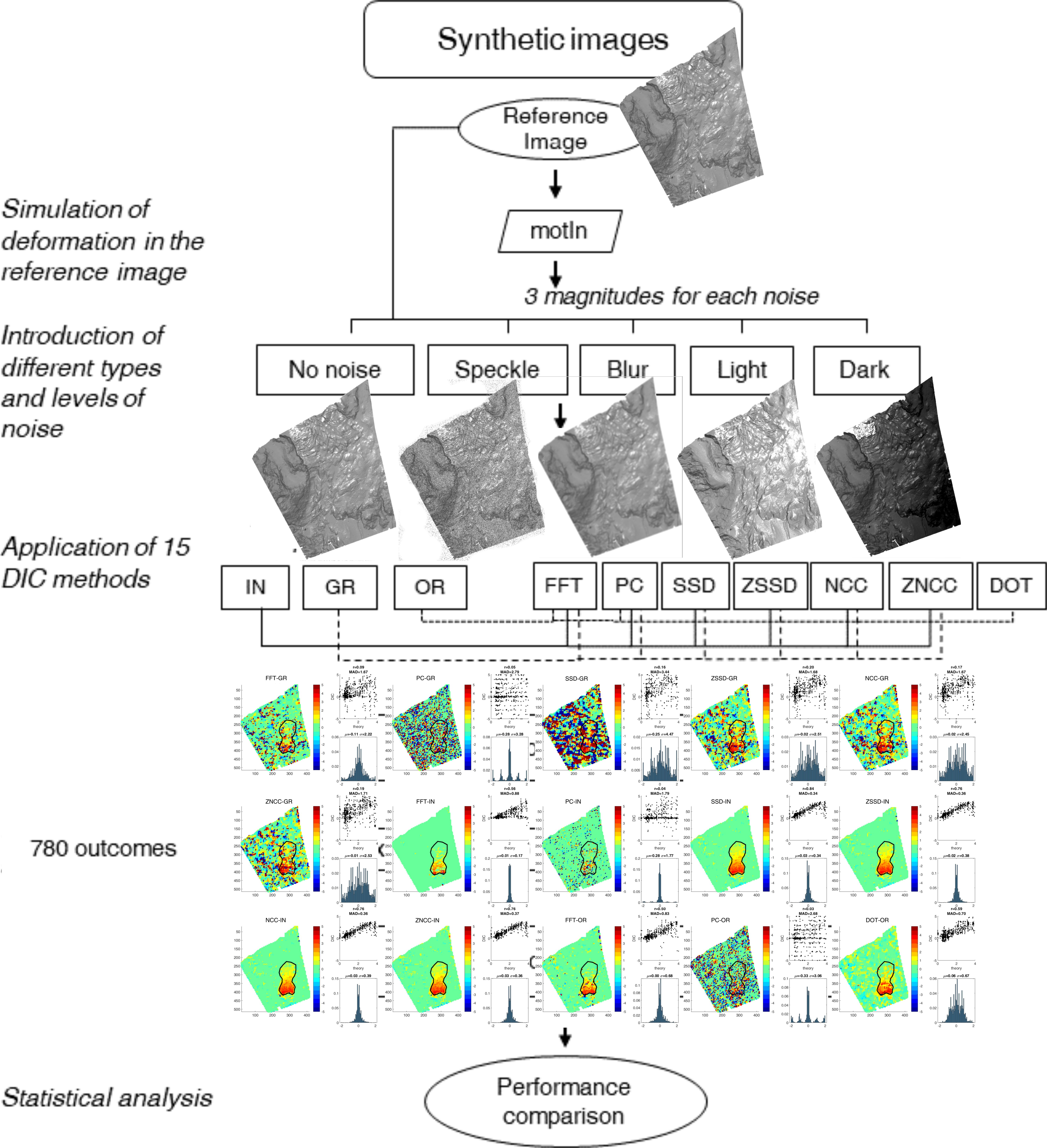
In this section, we describe the DIC methods used in the comparison and an original correlation function which can be applied to complex matrixes. In the second and third sections, we present the dataset to conduct the comparison of methods. We adopted synthetic and real images: we produced the synthetic images using a shaded relief of a real digital surface model (DSM). The adoption of synthetic images permitted to add artificial noise and to vary its type and magnitude. Also, the true displacement value was exactly known and thus, it was possible to assess the correctness of the DIC outcomes precisely. Furthermore, we used two sets of real images acquired by different sensors. The real images concern diverse environments in order to make the DIC comparison as much general as possible. Like in many practical surveys, we did not have available ground-truth measurements to validate the real images’ outcomes. Rather, the scope of using real images was to evaluate whether the influence of the noise observed in the synthetic cases came up also in the real images in a similar fashion. The final part of the section illustrates the metrics that we adopted as criteria for comparing the DIC method outcomes. The rationale of the study is shown in Figure 1.
3.1. Digital Image Correlation Methods
In our study, we considered three possible image representations: (1) image intensity (IN), (2) intensity of the image gradient (GR) and (3) image orientation (OR), to which we applied various similarity functions. Given an image intensity IN, the intensity of the gradient is defined as:
where are the first derivatives in the two directions. A GR image should be insensitive to changes of image intensity and to some extent, to changes of illuminations [20], but it could be more affected by noise [25].
The image orientation [26] is defined as:
An orientation image (OR) is complex and it is intrinsically normalised. As such, it is insensitive to changes of intensity and is robust against changes of colour and local illumination inhomogeneity. Fitch et al. (2002) [26] originally proposed their orientation correlation, which they calculated using the cross-correlation in the Fourier domain.
In its basic form, DIC provides the measurement of the bi-dimensional rigid translation of an image template. The rationale is to search for the position where a given similarity function reaches its maximum. is evaluated between a given reference template and multiple candidates of search templates within a search band. The search band is a wider area centred in the position of the reference template. For its characteristics, the process is often referred as to template matching, pattern tracking or similar.
Multiple correlation functions have been proposed in the literature. Among them, we considered the most commonly used in geoscience studies. One of the most popular is the (1) normalised cross-correlation (NCC) calculated in the spatial domain. We also examined the (2) zero-mean normalised cross-correlation (ZNCC). Two other methods are the (3) sum of squared differences (SSD), also known as the minimum quadratic difference [27] and the variant (4) zero-mean sum of squared differences (ZSSD). We considered two DIC techniques that operate in the frequency domain: the (5) cross-correlation calculated with Fourier transform (FFT) and the (6) phase correlation (PC). Finally, we included in the comparison an original method which is suitable to apply to complex matrixes, we named it (7) dot multiplication (DOT).
Concerning the correlation functions, NCC and ZNCC are defined as:
where is the position of the reference template in the image, is the position in the search area of the search template and are the mean values of the reference and search templates, respectively.
Both NCC and ZNCC are simple to evaluate, as they vary between −1 and 1 (respectively the worst and best matching); as such, they can be compared between different correlation attempts. However, large pixel differences can dominate the calculation. ZNCC is expected to perform better than NCC with respect to illumination changes.
An alternative to spatial cross-correlation is SSD [20,27] (and its variant ZSSD), which are simply defined as the Euclidean distance between two templates:
The best matching between the templates is found where and are minimum. SSD is not normalised and thus, it can suffer changes in image intensity. SSD and ZSSD are easily dominated by large pixel differences for their quadratic form. They both are rarely used in geosciences and are not expected to show great performances. However, we included them in our research for completeness.
We defined a new similarity function, DOT, which applies to complex matrixes, such as OR images. DOT is defined as follows:
where are the dimensions of the search area, while * denotes the complex conjugate. and are respectively the reference and search template of the OR image. The argument of the summation is the real part of the dot product of two complex numbers, which is equivalent to the cosine of the angle amid the two numbers. Therefore, the more the angle is small (i.e., the two numbers are similar), the more the cosine is close to one. DOT can assume values between −1 and 1 for the minimum and maximum similarity, respectively. Thus, it can be compared between multiple correlation attempts.
The computation of DIC in the spatial domain can be quite demanding. A much faster alternative is to operate in the frequency domain. We considered two frequency-based methods:
where and denote the Fourier transform and its inverse. FFT is equivalent to the spatial cross-correlation for the convolution theorem. FFT is not normalised and it can be sensitive to illumination changes. Alternatively, it is possible to ignore the signal amplitude and to consider only the phase correlation, PC [28]. The drawback of PC is that all the phase differences are weighted equally, while one would expect that the negligible components should have less weight [29].
Considering all the possible combinations of image representations and similarity functions, we examined the performances of 21 distinct DIC methods in total.
It is worth noting that the choice between the calculation of DIC in the spatial or frequency domain is not limited to the computational costs. In the spatial domain, the calculus is in the Lagrangian specification, i.e., the observer follows the reference template that slides in different positions within the search area and searches for the best matching between all the possible templates. On the contrary, the frequency domain implies an Eulerian approach. In the Eulerian approach, the observer is static and analyses the same area in two different times. This has two effects: first, since the considered templates are not exactly the same, but they are rather a portion of each other, decorrelation might occur for relatively large displacement [30]. Second, the maximum displacement that can be detected is equal to half the size of the search template for the Nyquist criterion.
To achieve subpixel accuracy, we used the approach proposed by Travelletti et al. (2012) [11] for every DIC method. We up-sampled of a given factor the similarity surfaces with cubic interpolation, using the Matlab function interp2. Then we search for the maximum of the interpolated surface. In our study, we used an up-sampling factor of 25.
Where not expressed differently, we calculated the DIC with four template sizes: 8 × 8, 16 × 16, 32 × 32 and 64 × 64 pixels. When computing DIC in the spatial domain, we used search bands of half the template side’s size in every direction (i.e., 4, 8, 16 and 32 pixels). Thereby, the range of possible detected displacement was the same as for the DIC calculated in the frequency domain.
3.2. Synthetic Images and Noise
To conduct a formal comparison of DIC methods, we used synthetic images that we could freely manipulate. We created a series of images where we introduced simulated deformation and noise. Thereby, the real displacement was exactly known and we were able to evaluate the outcomes’ correctness. We produced a 540 × 434 px shaded relief based on a DSM of a natural slope. Characteristics and geographical context of the DSM are shown in Figure S1 from the Supplementary Materials. The lighting position of the shaded relief has been set to (0°, 90°) (azimuth, elevation). The intensity range of the reference image (refIm) varied between [0, 255]. Then, we moved the pixels within a region of interest (ROI) using non-linear transformations, in the form:
where motIm is the image with simulated motion and outside the ROI. According to Equation (7), the produced displacement is not a rigid translation, but it is a non-linear surface deformation that simulates real cases. Therefore, within every template couple in the DIC calculus, displacement gradients are present. Before to apply Equation (7), we upsampled the images of a factor of 10. Subsequently, we resampled to the original size. Thereby, we were able to simulate a 1/10th pixel displacement. We conducted the resampling operation using the imresize Matlab function using bicubic interpolation.
Then, we introduced various types and magnitudes of noise into motIm (Table 1): (i) speckling, (ii) blurring, (iii) different positions of light source and iv) illumination intensity changes. The Speckle noise is defined in the form , where n varies uniformly with mean 0 and a given variance. We considered speckle variances of 0.03, 0.05 and 0.07. The Blur noise has been produced with a low-pass mean filter of different sizes: 3 × 3, 5 × 5 and 7 × 7 pixels. We simulated Light noise by using three positions of the light source to create the shaded relief: (10°, 80°), (30°, 60°) and (50°, 40°).
Light noise is feature-based spatially-coherent noise. The Dark noise has been produced by subtracting from the intensity image an oblique plan that linearly varied from 0 to 100, 0 to 150 and 0 to 200 (from left to right). Examples of synthetic images are shown in Figure 2. The considered noises concern typical disturbing effects that might occur in real surveys. Light noise well simulates the shadow pattern change caused by the different sun position or the presence of isolated clouds. In contrast, Dark noise represents homogeneously-varying illumination intensity. These are known issues in operative surveys [7,11,12,17,31]. Blur noise simulates image defocusing that can occur for many reasons: e.g., incorrect manual or autofocusing, low illumination, presence of haze or precipitation, condensation of the optical objective or camera vibration. To our knowledge, the influence of image defocusing has never been studied, but, according to our experience, it is a quite frequent disturbing effect. Finally, Speckle is a pseudo-random multiplicative noise that is typical of coherent waves. Probably, this phenomenon is less recurring in visual-based surveys. However, it can occur when DIC is applied to satellite SAR images [32]. We did not use combinations of different noises because the aim of our study was to evaluate the influence of specific disturbances on the DIC calculation.
In total, we analysed 13 versions of motIm with different types and levels of noise (Figure S2). The DIC was calculated on a regular grid of 8000 nodes and the ROI contained 628 nodes.
3.3. Real Images
We conducted a similar analysis using real images acquired in natural environments (Table 2). We considered two examples of image data adopted in DIC applications. We used ground-based photographs of an Alpine glacier and satellite panchromatic images of a desertic area. These sites concern diverse environments, but both characterised by high ranges of deformation, with a maximum displacement of ~10 px.
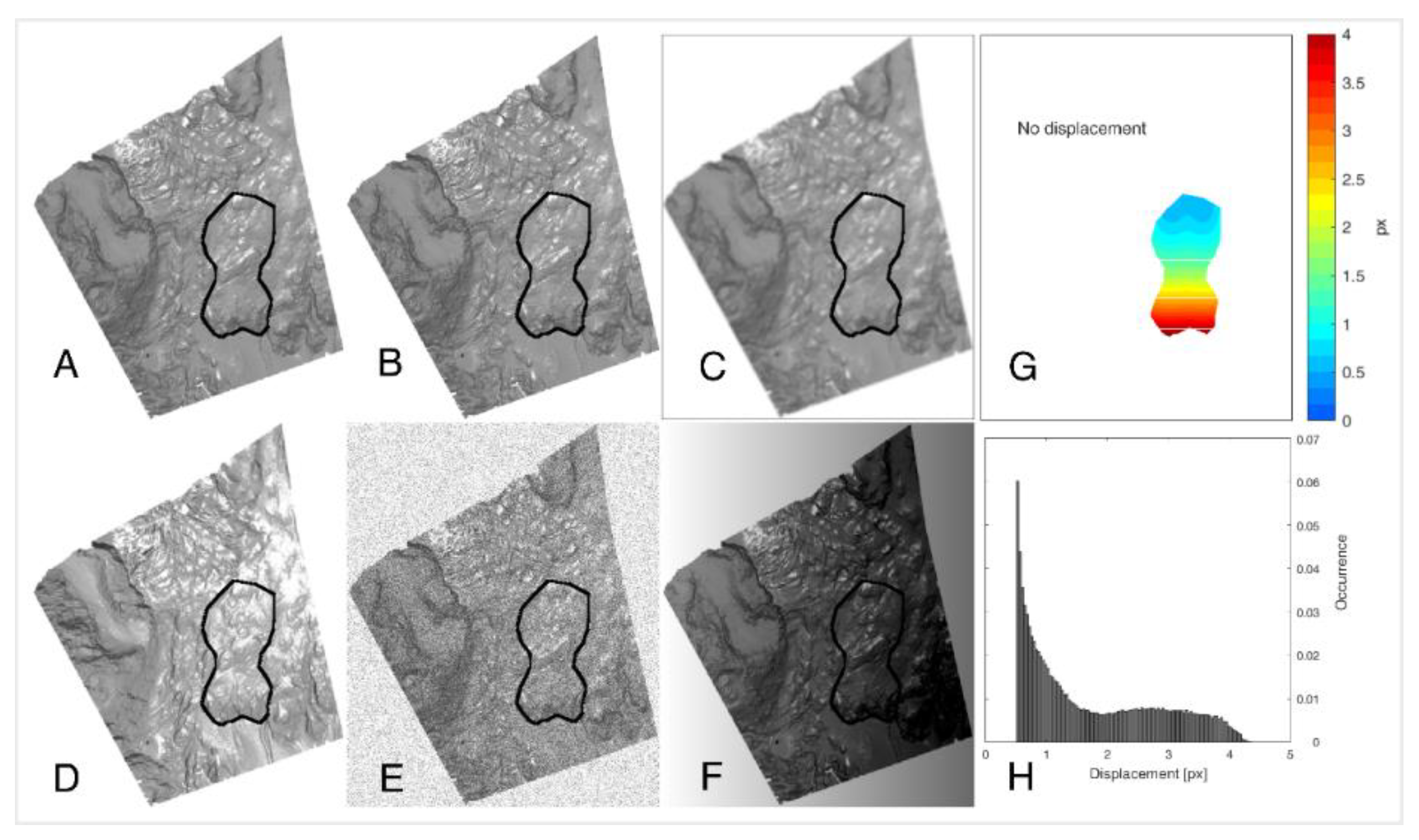
The ground-based dataset refers to oblique 18 Mpx photographs of the Montitaz Lobe of the Planpincieux Glacier (PG), in the Mont Blanc area [31]. The reference image was acquired in optimal conditions in 27 September 2019 at h12.00. To assess the different methods’ performances, we calculated the DIC using three distinct search images that have been acquired in 28 September 2019 at h12.00, h08.00 and h19.00 (Figure 3). Therefore, respectively with (1) same illumination conditions, PGopt; (2) different light source position, PGlight and (3) different illumination intensity, PGblur. In PGblur, the scarce illumination also introduced a slight blurring.
Between the acquisitions of the reference and the other three images, some snow melting occurred in the upper part of the images, while a small ice break-off detached from the glacier terminus. We were able to evaluate the robustness of different DIC methods also against these kinds of disturbance. We adjusted the displacement in order to normalise the different time gaps between the three couples of photographs. The DIC processing was conducted using 64 × 64 template size.
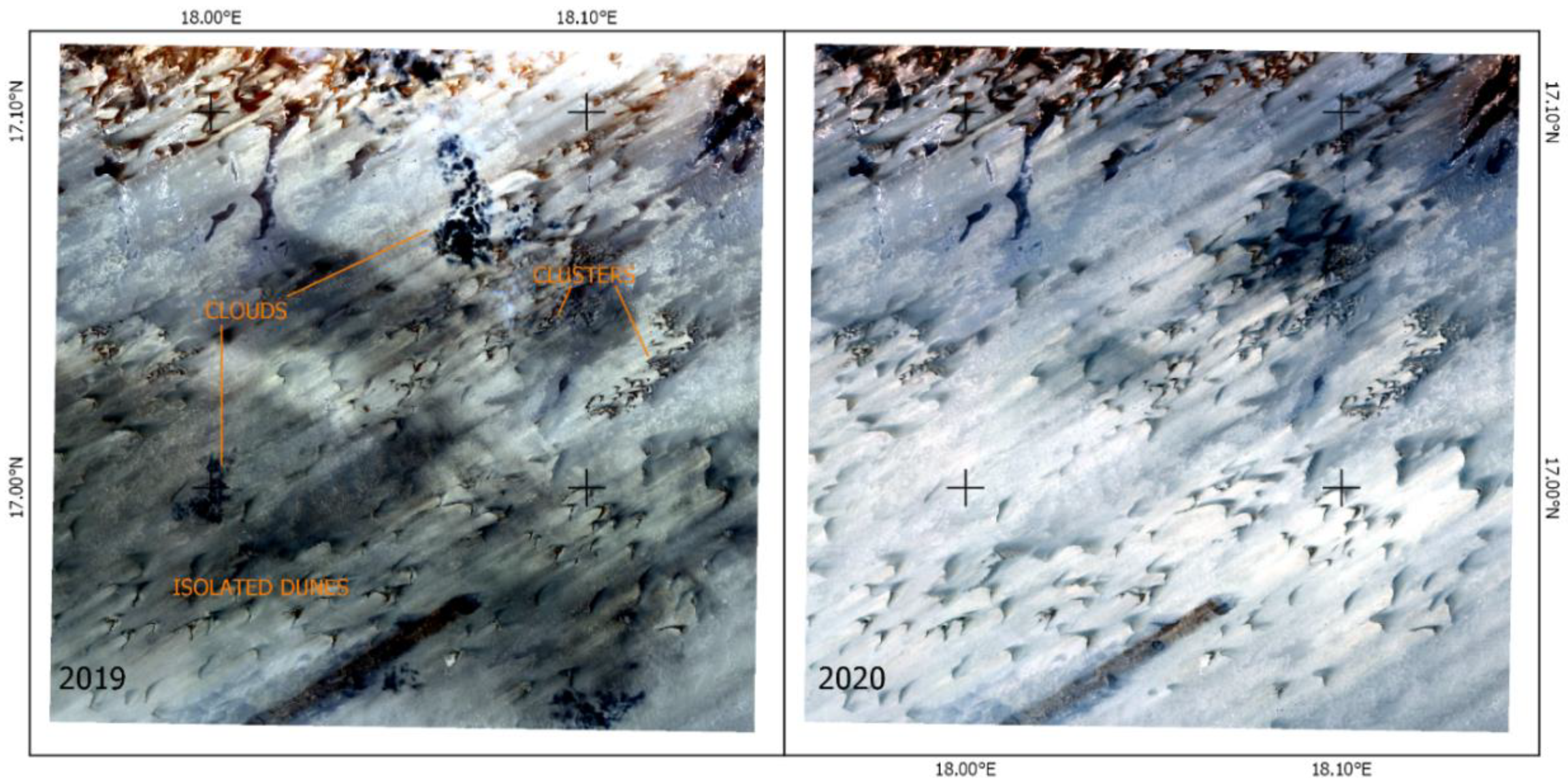
The satellite dataset is composed of a pair of Sentinel 2B images (image codes: T33QZU_20191008T090849 and T33QZU_20201002T090719), which targeted the Bodélé Depression (BOD) in Chad [33]. We considered a portion of 400 km2 centred approximately in 17.02° N–18.02° E. Such an area presents isolated sand dunes and clusters of small dunes and a homogeneous background (Figure 4). The environmental conditions of the first image showed strong wind and partial cloudiness. Therefore, the image appeared slightly blurred and the illumination was not uniform. We applied the DIC using templates of size 32 × 32 and 64 × 64 px.
To the real images, we applied four exemplar DIC methods (1) FFT-OR, (2) DOT-OR, (3) ZNCC-IN and (4) PC-GR.
3.4. Criteria for the Comparison
To evaluate the performances of the DIC methods, we used specific criteria for the comparison. Since the true displacement is known in the synthetic case, we defined a series of quantitative metrics. By contrast, in both the PG and BOD cases, ground-truth measurements were not available. Therefore, we conducted a qualitative analysis based on the visual identification of outliers, spatial resolution and displacement pattern.
The metrics adopted to examine the results obtained with the synthetic images are the following. Outside the ROI, where the theoretical displacement is zero, we calculated mean (μ) and standard deviation (σ) of the displacement as an estimate of accuracy and precision. In motIm, (μ) and (σ) are ideally zero. However, since the displacement is evaluated on templates that can be over the ROI limits, non-zero values could verify in the neighbourhood of the ROI. This behaviour is expected to be more evident with larger templates. Within the ROI, we calculated the mean absolute difference (MAD) and the linear correlation coefficient (CORR) between the obtained displacements and the mean theoretical displacement included in the template. We considered the mean value because the displacement is not uniform within the templates and the DIC measures a sort of averaged displacement [18]. For this reason, the DIC might misestimate the real displacement. We investigated this aspect considering the bias between the 1st, 2nd and 3rd quartiles of the distributions of the measured and theoretical displacements.
We noticed that sometimes, even though the overall quality of the results was good, the presence of a few outliers in the residuals strongly affected in a negative way the MAD and CORR metrics. Therefore, we decided to analyse the results also excluding the outliers (MAD* and CORR*). Usually, these outliers concern areas near the ROI boundaries where the investigated templates lie over the ROI edges. When this happens, no displacement is detected near the ROI boundaries. We refer to the ability to correctly identify the displacement in the ROI limits’ vicinity as “spatial resolution”. Simultaneously, we reported the percentage of outliers (%OUT) in the results. We defined an outlier a value that is more than three scaled median absolute deviation (sMAD) away from the median, where sMAD is defined as ∼1.5 median . According to the outlier definition, this metrics has to be evaluated carefully. A small number of outliers could entail a very scattered distribution of the residuals and therefore results of low quality. However, a large percentage of outliers is certainly an indicator of poor performances.
Since we are presenting a certain amount of data, the reader might find hard to examine all the results. Therefore, besides the quantitative parameters, we defined a simple qualitative metrics which assigns a negative/neutral/positive score depending on the visual analysis of the results. We used the following notation: a minus (−) is given when the results contain so much noise that the displacement pattern is not yet recognisable or the pattern is still recognisable, but the values are strongly over/underestimated or the spatial resolution is very poor. A zero (o) is assigned when the displacement pattern is maintained and the values are approximately correct, but many outliers are present. A plus (+) is assigned when the results show good spatial resolution, the displacement values and pattern are correct and the number of outliers is limited.
Finally, we examined the computational time required to operate the various DIC correlations. Even though the computational time is not related to the quality of the results, it is an important parameter that can be relevant in applications that require fast processing or that have to elaborate very large amount of data.
4. Results
In this chapter, we present the results of 15 DIC combinations of correlation functions and image representations. Every combination has been applied to 13 images characterised by various noise types and magnitudes. The analysis has been conducted using four distinct template sizes. In total, we compared 780 results. Furthermore, we examined the results of four model DIC approaches (i.e., ZNCC-IN, DOT-OR, FFT-OR and PC-GR) applied to four couples of images of various real environments. The results of NCC, ZNCC, SSD and ZSSD in combination with OR image provided poor results and they will be not shown. Since DOT is valid for complex numbers, it has been applied exclusively to OR images.
4.1. Methods’ Comparison Using Synthetic Images
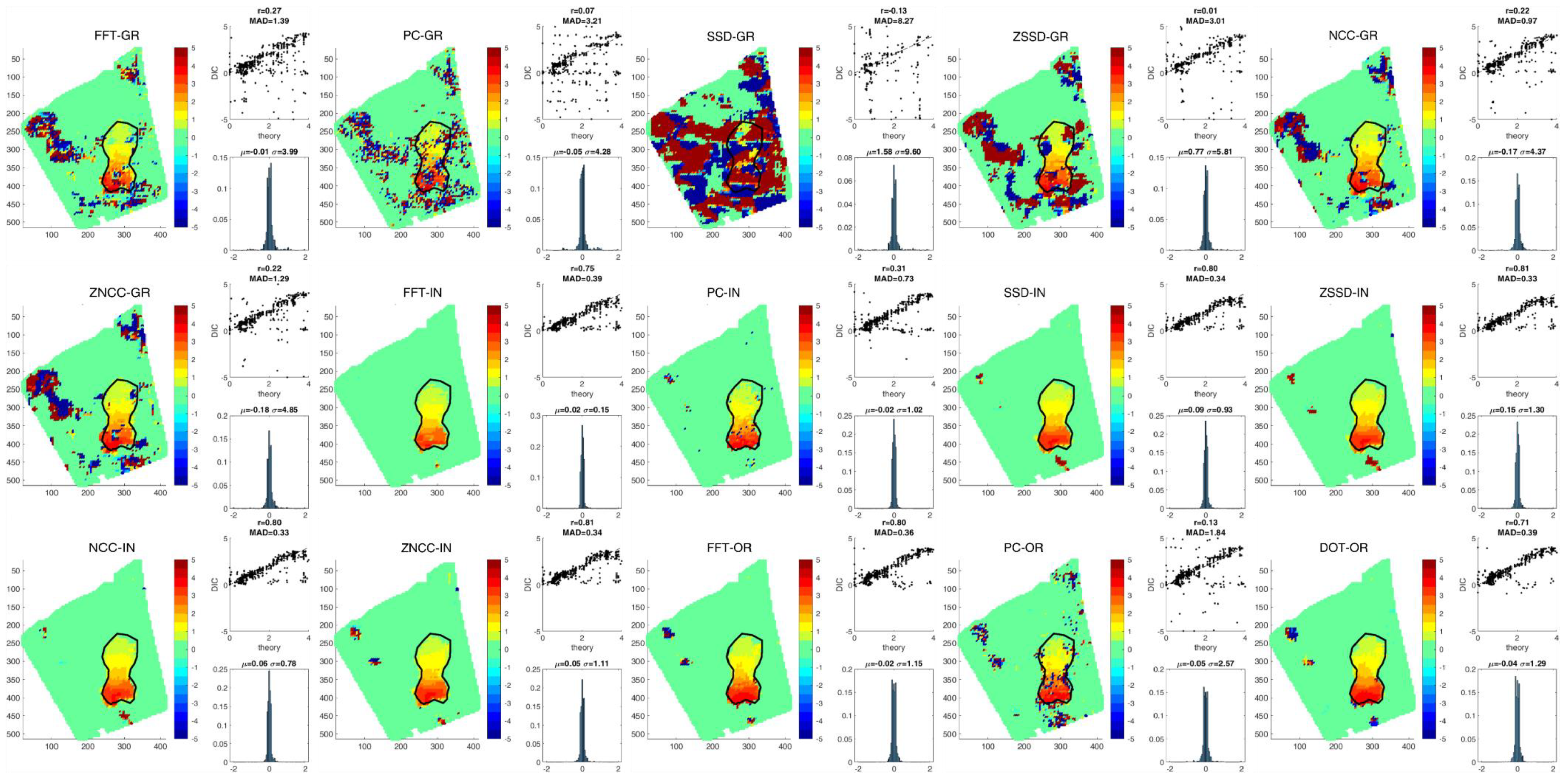
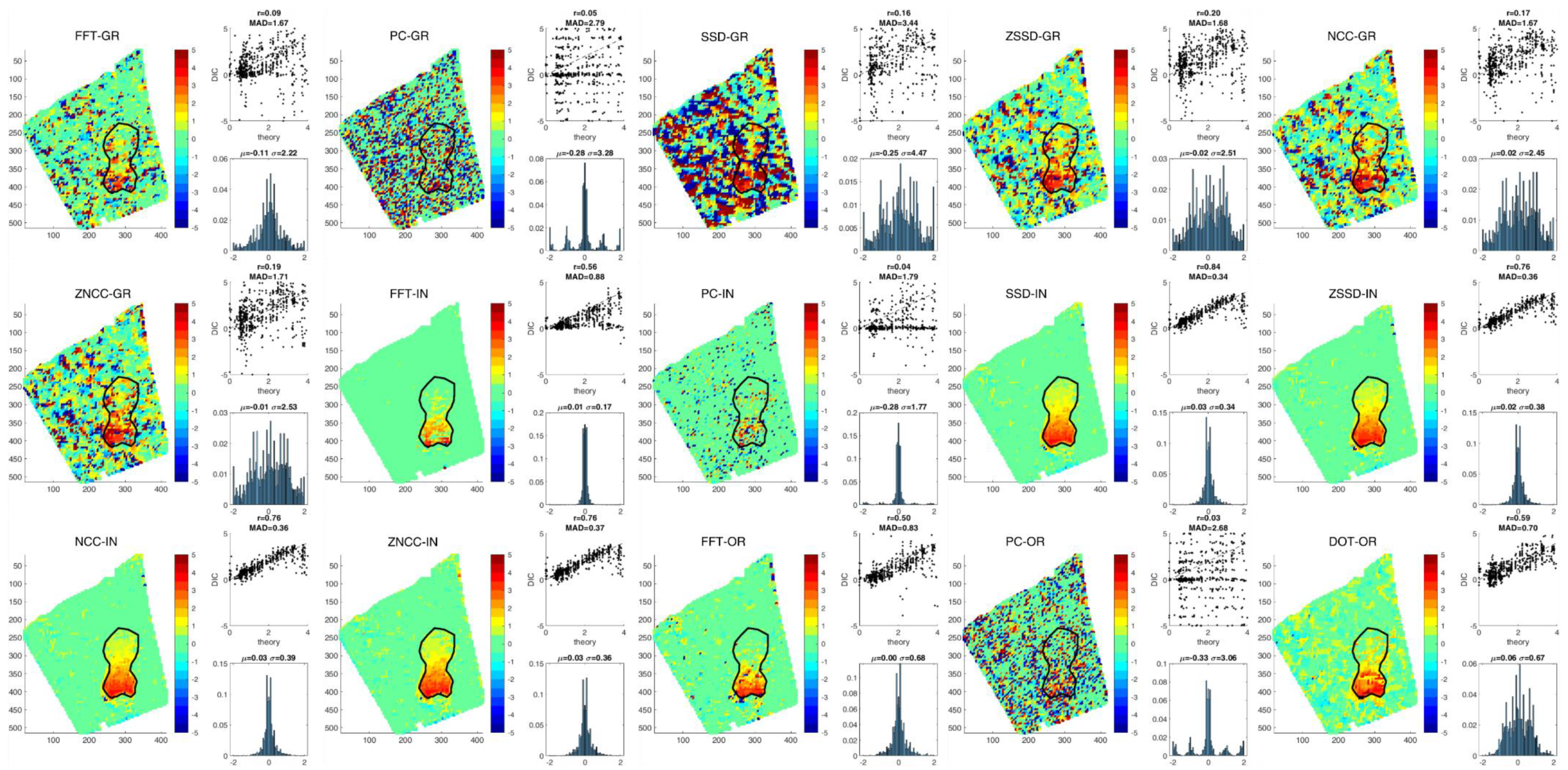
In the following, we shall present the results obtained with the considered DIC methods applied to the synthetic images. In Figure 5 and Figure 6, we report the displacement maps, the distributions of the displacement of the stable areas and the scatterplots between the measured and theoretical data obtained with every DIC combination for (i) Speckle3 noise calculated with 32 × 32 template size and (ii) Blur5 calculated with 16 × 16 template, respectively. In these figures, we also report the values of CORR, MAD, μ and σ. In Figure S3, we report analogue figures concerning every combination of the correlation function, image representation, noise and template size (i.e., 780 outcomes).
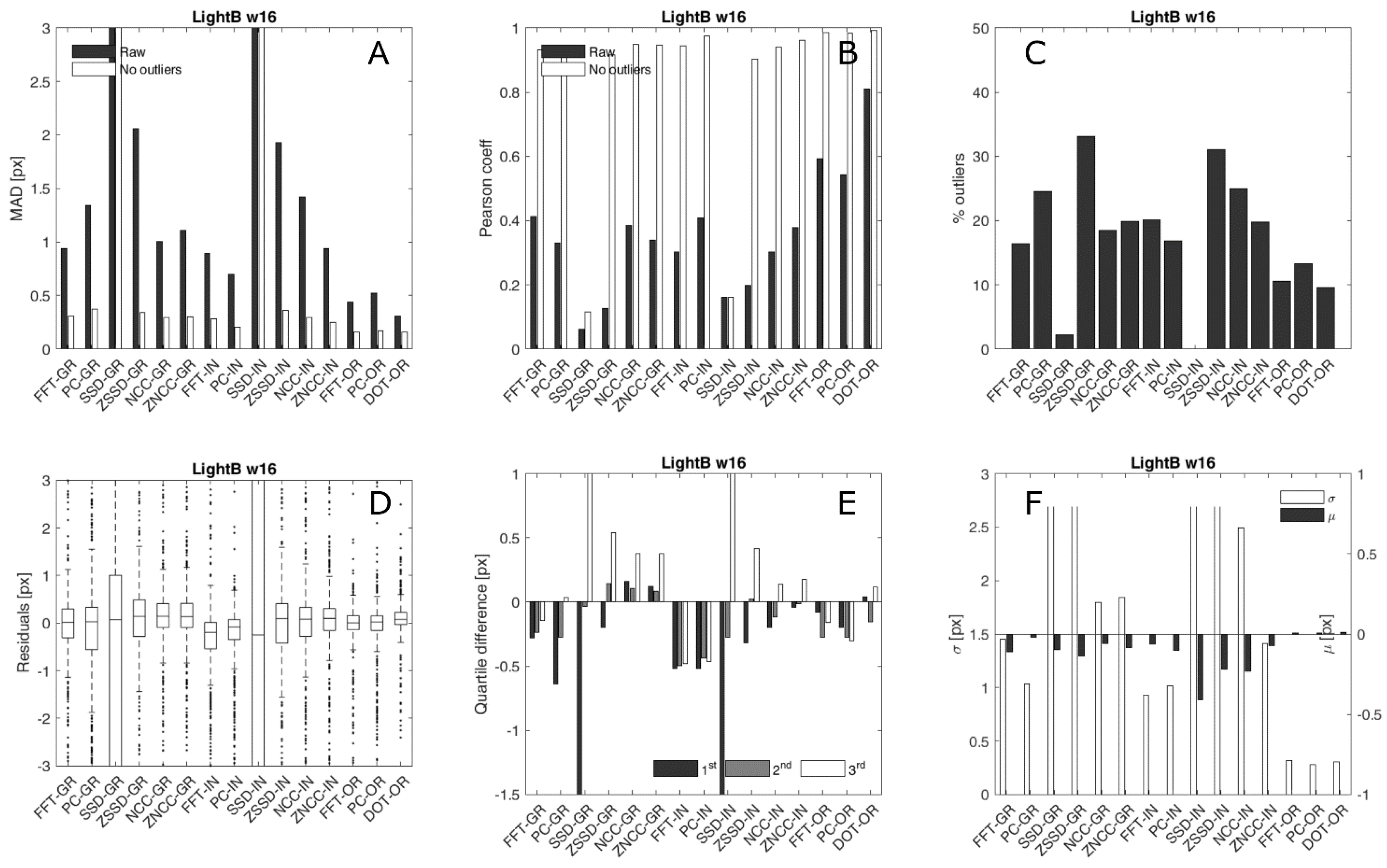
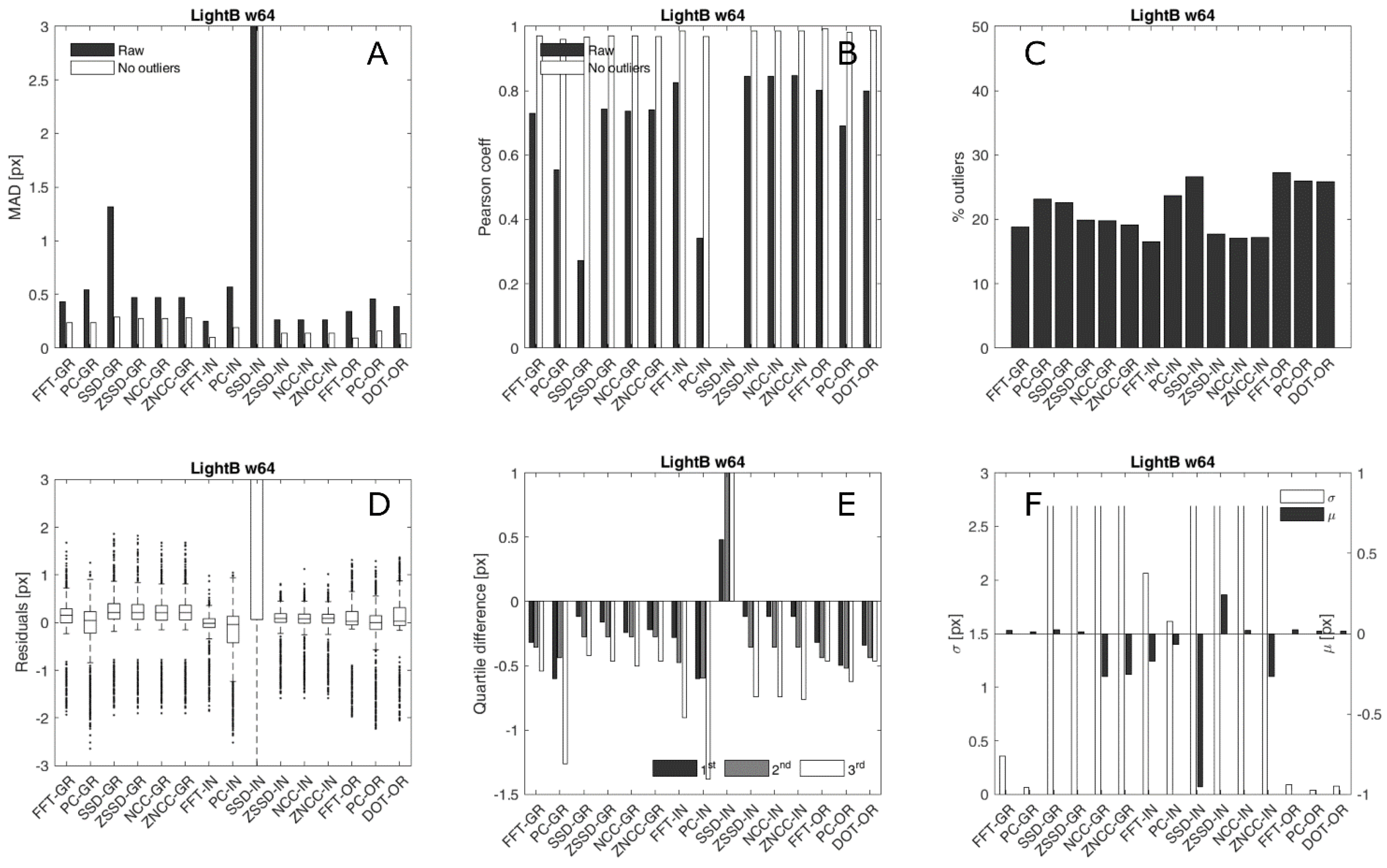
Besides, we prepared a series of figures containing the metrics present in Section 3.4. An example is presented in Figure 7 and Figure 8, which show the outcomes of LightB noise calculated with 16 × 16 and 64 × 64 template size, respectively. We realised one similar figure for every combination of noise type and magnitude and template size (i.e., 42 figures). All the figures can be found in Figure S4.
In Table 3, we report the qualitative metrics based on the visual analysis of the displacement maps. The rightmost column contains the sum of the scores obtained with each template size.
Image intensity. DIC applied to IN image provides the best results in the presence of Blur and Speckle noise. On the other hand, Light noise can provoke large pixel differences that can influence the correlation calculus. Dark noise introduces a bias that affects non-zero-centred correlation functions.
Image gradient. The use of GR images provides poor results in the presence of Blur and Speckle noise. On the contrary, GR images appear less affected by Light noise and are almost unaffected by Dark noise. GR images return acceptable outcomes only using NCC and ZNCC correlations. With large templates, GR images provide a lower spatial resolution compared to the other image representations. The outcomes obtained with GR images are concentrated on integer displacement values, especially when combined with PC.
Image orientation. OR images yield very high performances in combination with DOT technique. Also, FFT and PC return better results when applied to OR images than IN and GR cases. OR is unaffected by Dark noise and it is resistant against Light noise.
FFT and PC. The performances of frequency-based methods with templates of size 8 × 8 are poor because the displacement is relatively large with respect to the template size. Therefore, signal decorrelates. This is more evident for IN images. However, FFT correlation performs generally better compared to PC for every template size and in combination with every image representation. A remarkable observation is that the frequency-based methods underestimate the displacement. The underestimation is more evident for IN images with Blur noise. The degree of underestimation seems independent from the template size (Figure S4).
NCC and ZNCC show similar results. However, since NCC is calculated using values that are not centred in zero, it is very affected by changes of illumination, because the difference of the mean value of the image can dominate. Therefore, NCC performs badly with Dark noise. Both NCC and ZNCC provide accurate values of displacement. However, in the presence of Blur noise, the spatial resolution decreases and they tend to spread the displacement when calculated with large templates (Figure S3).
SSD and ZSSD. SSD is the weakest method among those considered. It performs acceptably only for IN images and slight Blur noise. However, the subtraction of the template mean value allows at reducing the impact of the quadratic term. Accordingly, ZSSD shows results similar to NCC and ZNCC. Nevertheless, it is less performing when applied to GR images. ZSSD is less robust against Speckle noise, in particular when calculated with small templates.
DOT works with OR images and it is more performing than FFT-OR and PC-OR. DOT is unaffected by Dark noise and very robust against Light noise. It performs similarly to NCC in the presence of Speckle and limited Blur noise. Poor results are obtained in the presence of strong blurring. DOT results are quite smooth and the fraction of outliers is generally lower compared to other methods.
In Figure S5, we report examples of IN images of motIm with and without noise. Besides, we show also the power spectra of each image. In this analysis, we considered only the bounding box of the ROI. We report the same analysis for GR and OR images in Figure S5. The power spectra of motIm IN and GR are similar, while in that of OR, the signal appears less defined. Blur noise smooths the edges and makes the image features less clear. This is particularly evident in GR image. The spectra of every blurred image representation have lowered high frequencies. Dark noise does not influence GR and OR images and their power spectra, while it introduced a bias in IN, as expected. Light noise tends to strengthen the features in GR image, while OR image seems to maintain the main pattern. Speckle noise introduces random scattered noise, which makes OR and GR images more disturbed. With Speckle noise, the higher frequencies strongly increase their power in IN and GR images. In general, higher frequencies of OR spectra are less influenced by any kind of noise.
4.2. Methods’ Comparison Using Real Images
The maps of the vertical displacement component of the PG images are shown in Figure 9. From left to right, the columns report the results obtained with DOT-OR, ZNCC-IN, PC-GR and FFT-OR techniques. The results of PGopt, PGlight and PGblur images are reported respectively in the upper, middle and lower row. As one can note, the performances with PGopt images are approximately the same for every DIC method. PC-GR map is less smooth and several scattered outliers are present. In the upper part of the image, some noise appeared in the maps obtained with every DIC method, in correspondence of fresh snow melting (Figure 3). However, DOT-OR and FFT-OR appear less affected by this phenomenon. Similarly, DOT-OR and FFT-OR perform better with PGlight images. In this case, DOT-OR is slightly more performing compared to FFT-OR. ZNCC-IN and PC-GR are both influenced by Light noise, but the effects are different. In general, PC-GR shows scattered outliers, while ZNCC-IN decorrelates in the form of stains. DOT-OR, ZNCC-IN and FFT-OR methods performed equally well with PGblur images. They show lower displacement values compared to those measured with PGopt images. However, ZNCC-IN underestimates at a slightly less extent compared to the other methods, especially in the horizontal component (Figure S6). The underestimation confirms the observations obtained with the synthetic images, even though a slight slowing down of the glacier motion cannot be excluded. PC-GR results with PGblur images are quite poor. All the DIC methods decorrelate in the area corresponding to the break-off.
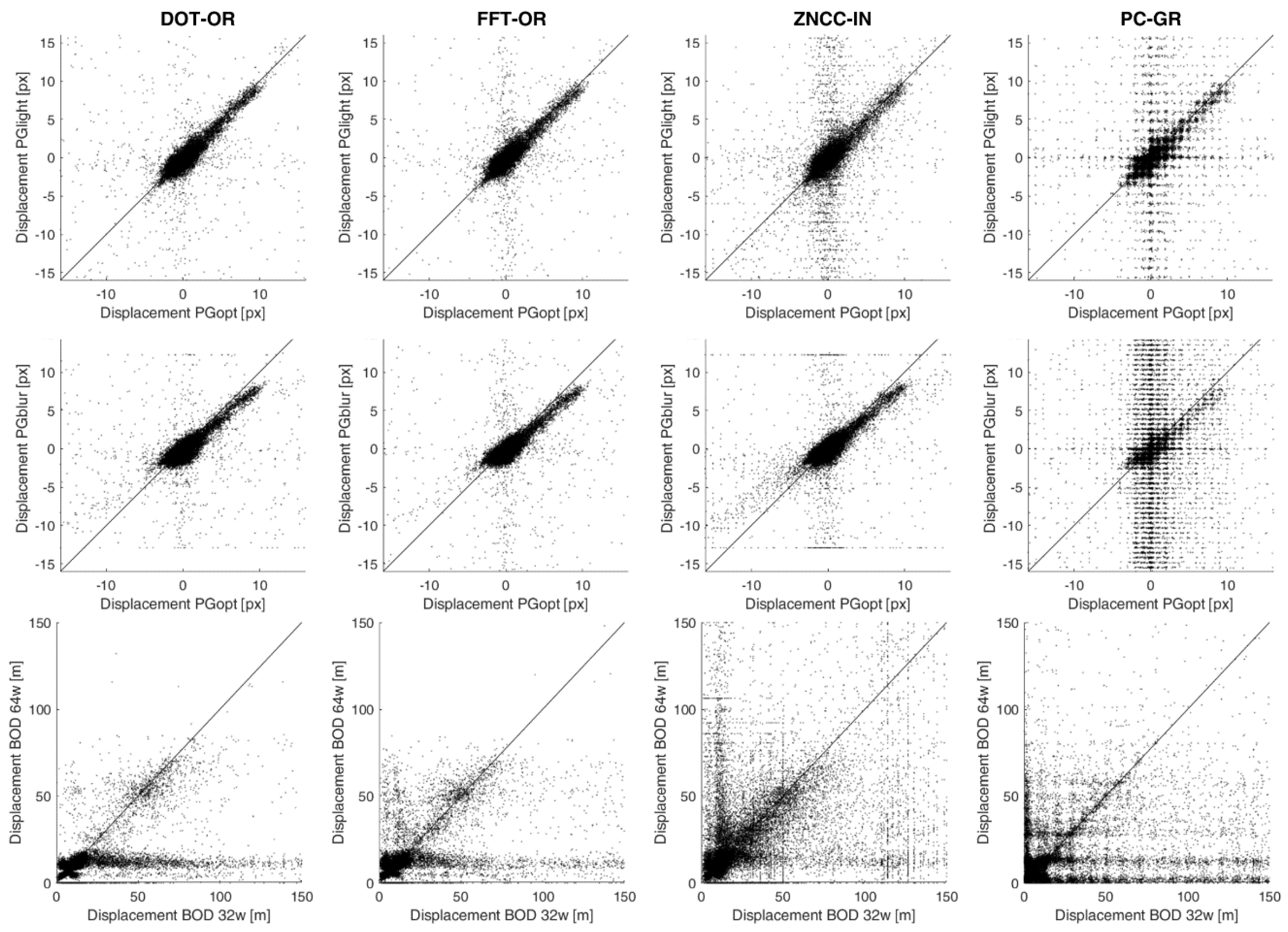
In Figure 10, we report the scatterplot of the outcomes obtained with PGopt images, which can be considered as reference, versus the outcomes of PGlight and PGblur. It is evident that DOT-OR and FFT-OR behave almost equally with all the images, while ZNCC-IN shows some random noise with PGlight images. PC-GR performs satisfactorily with PGlight, while most of the results with PGblur appear random. PC-GR outcomes present a regular grid-like distribution.
The results of BOD images partially follow those of PG. Concerning the outcomes obtained with the template of size 32 × 32 (Figure S6), DOT-OR and FFT-OR show similar results. The contours of the largest dune clusters are well defined and the presence of outliers very limited. Both methods detect single dunes, but with a narrow spatial resolution. On the contrary, ZNCC-IN identifies the displacement of small isolated dunes, but it presents scattered outliers. With PC-GR, the areas corresponding to the dunes appear as clusters of random noise and only the displacement of the largest groups of dunes is correctly measured. The presence of clouds strongly impacts over ZNCC-IN, while DOT-OR and FFT-OR appear almost unaffected. The inhomogeneous illumination does not alter the results of FFT-OR, PC-FR and DOT-OR significantly, while ZNCC-IN fails in correspondence of the edges of the shadows cast by the clouds.
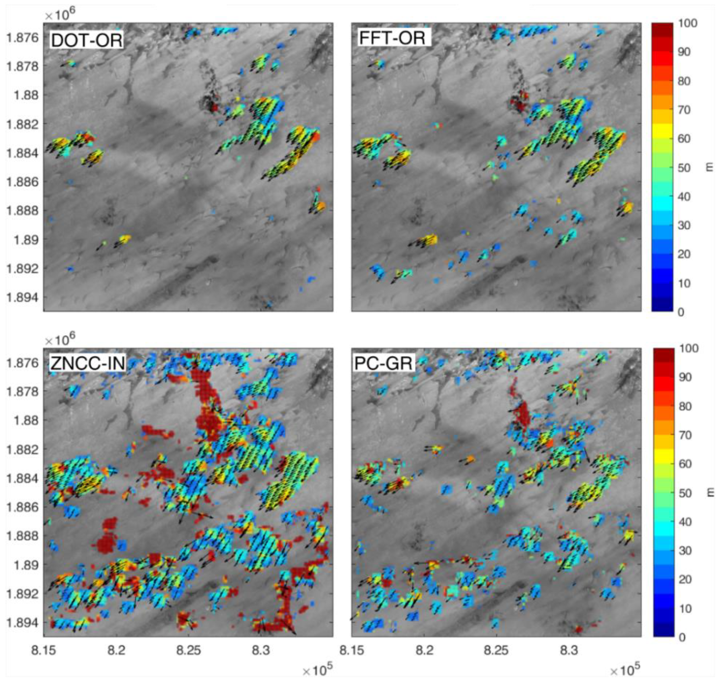
The outcomes obtained with 64 × 64 template size are slightly different (Figure 11). DOT-OR and FFT-OR show very smooth maps. The largest groups of dunes are correctly identified with good spatial resolution. However, the smallest dunes are not entirely detected, especially by DOT-OR. Any trace of the cloud presence does not appear in these cases. In the ZNCC-IN maps, the noise is slightly lower compared to that of 32 × 32 template. However, outliers remain in correspondence of clouds and shadows. The displacement of the isolated dunes is identified, but it is largely spread around in the form of stains. PC-GR performs better compared to the case with 32 × 32 template. All the dunes are identified and the spatial resolution is fair, but the displacement appears slightly underestimated. The presence of outliers is significantly reduced and are much less than in ZNCC-IN results. Like ZNCC-IN, the displacement appears slightly spread around the dunes, but at a smaller degree.
The scatterplots in Figure 10 show that the adoption of 64 × 64 template with DOT-OR, FFT-OR and PC-GR reduces notably the occurrence of displacements greater than 70–80 m, which are very likely errors. On the contrary, the displacement distributions of ZNCC-IN remain almost the same and show a strong presence of outliers using both 32 × 32 and 64 × 64 templates. Like in PG images, PC-GR outcomes present a regular grid-like shape.
4.3. Computational Time
According to our analysis, the computational complexity varies largely depending on the domain where the correlation is calculated. We examined the aspect of the computational time using random templates of size 8 × 8, 16 × 16, 32 × 32 and 64 × 64 px. For the space-based correlation methods, we used search bands of half the size of the template. The results are shown in Figure 12. We used an eight-core CPU AMD Ryzen 7 1800X. SSD is the fastest method among the space-based ones, while NCC, ZSSD, DOT and ZNCC are approximately 2, 3, 4 and 6 times slower, respectively. We observed that the computational time of NCC, ZSSD and DOT tend to uniform for large sizes. On the other hand, frequency-based functions require a computational time three to five orders of magnitude lower, depending on the template size.
It is worth noting that the computational time of space-based methods depends mostly by the size of the search band. Probably, most of the circumstances do not require as large search bands as those we used in this experiment.
5. Discussion
The results of our experiment using synthetic images demonstrated that IN images are quite resistant to Blur and Speckle noise. Nevertheless, frequency-based methods still fail in the presence of blurring, probably because it introduces strong low-frequency components that dominate over the high-frequency features. On the other hand, IN images are more sensitive to Light noise, because it can produce coherent areas of large pixel difference. GR images do not suffer changes in illumination and they provide acceptable results in the presence of Light noise. However, they are more sensitive to Blur and Speckle noise, in accordance to the observation of Sjödahl [25]. This could appear in contrast with the findings of Martin and Crowley [20], which observed more stable correlation indexes using GR images. However, their study was only focused on index stability, rather than on the results’ effectiveness. We noticed a peculiar behaviour of PC-GR method. The obtained displacements were concentrated on integer values (the dimension of one pixel of Sentinel-2 images is 10 m). This occurs because the autocorrelation function of GR images has a narrow prominent peak which makes the signal well-defined [25]. However, such a sharp peak probably concentrates all the information into integer shift values. As a consequence, GR images are less suitable for detecting sub-pixel displacements. OR images behave similarly to GR, but they return much better results. Since OR images are complex, a single element of the matrix is composed of two components. Therefore, OR images contain more information compared to IN and GR. Consequently, the original pattern information is less corrupted by noise and the signal-to-noise ratio maintains higher.
Concerning the correlation methods, space-based correlations non-centred in zero (i.e., SSD and NCC) fail in the presence of a change in illumination. Results strongly improve by considering the zero-mean values and adopting normalised function. As a matter of fact, ZNCC outperforms the other space-based methods. In general, SSD and ZSSD are more sensitive to large pixel variations, because the quadratic form enhances the largest differences. Among the space-based correlations, SSD appears the least effective method, particularly when adopted with GR images. This result differs from the finding of Martin & Crowley (1995) [20]. A possible reason, as also suggested by Pust [22], is that they analysed the performances of SSD without any source of noise. NCC and ZNCC return similar results, but NCC strongly suffers changes of average intensity using IN images. Space-based methods fail when applied to OR images. Probably, this happens because OR images are complex and the space-based functions are well defined only for real numbers. In general, we observed that space-based methods (excluding SSD in general and NCC for Dark noise) are more robust compared to frequency-based ones, confirming the observations of Pust [22]. On the other hand, Bickel et al. [19] obtained slightly better results with FFT compared to ZNCC using large template size.
Formally, DOT correlation is calculated in the space domain, but we describe its behaviour individually for two reasons: first, it differs from classical space-based functions as it operates with complex numbers; second, we want to highlight the high performances of this original method that we developed. In principle, DOT may be applied to whatever image representation composed of two separate components: e.g., the first derivatives of the image intensity (like in this study) or two different bands of multispectral images. This opens new possibilities of investigation for defining original DIC approaches. In general, DOT-OR appears quite robust against every source of considered noise. It is unaffected by dark noise and it provides the best outcomes in the presence of Light noise. We observed acceptable results with Speckle and weak Blur noise. The higher performances of DOT probably depend on two elements: (i) DOT applies to OR images, which are less corrupted by noise and (ii) DOT correlation operates in Lagrangian specification. Therefore, it is less sensitive to decorrelation respect to frequency-based methods [30].
Compared to space-based methods, normalisation worsens the performances of frequency-based correlations. Indeed, FFT outperforms PC in every situation we examined. Probably, this happens because in PC, the contribution of the amplitude signal is ignored and all the phase components have the same weight in the correlation calculus. Therefore, the presence of noise that alters the frequency spectrum can easily limit the performance of PC. Similarly, Heid and Kääb [18] observed better outcomes from FFT, especially in the presence of homogeneous texture. Probably, as suggested by Lewis [29], since in PC all the frequencies are weighted equally, it fails when a predominant frequency is lacking, which is the case of homogeneous areas. As a consequence, PC is more prone to artefacts. We observed a general underestimation of frequency-based methods. Heid and Kääb [18] noticed the same behaviour in areas with the presence of displacement gradients. They suggested that this occurs because the features that move slower change less their texture (i.e., they decorrelate to a lesser extent). Therefore, the slower features’ contribution weights more in the correlation calculus. This hypothesis seems confirmed by the fact that the underestimation is less evident in OR images, whose intrinsic normalisation limits this effect. Frequency-based correlations suffer limitation concerning the template size. In our experiment, both FFT and PC failed when applied with 8 × 8 templates. Theoretically, the dimension must be at least twice larger as the maximum displacement for correctly detecting it. In practice, Bickel et al. [19] suggested as a rule of thumb to use a template size 6 to 17 times larger than the maximum displacement. We observed acceptable results with templates four times larger than the maximum displacement.
It is worth noting that normalised functions (i.e., PC, NCC, ZNCC and DOT) have the advantage of outputting an image-independent similarity index. This permits to compare the results between different attempts of the DIC calculus [18] and makes the similarity matrix much easier to understand. For example, this may allow to define heuristic criteria of data quality and help in the outlier detection [7].
The outcomes obtained with PG images agree with those observed with synthetic images. DOT-OR and FFT-OR return similar high-quality results. ZNCC-IN performs well with PGopt and PGblur, but it suffers the Light noise in the PGlight images. This confirms the lower robustness of the IN images against Light noise, as also observed by Dematteis et al. [17], who analysed the effects of lighting change using FFT-IN approach. Besides, ZNCC-IN fails in the areas where snow melting occurs, as already noticed by Heid & Kääb (2012) [18]. As expected, PC-GR shows acceptable results with PGlight images, as it is less affected by Light noise, while it totally fails with PGblur.
On the other hand, the outcomes of BOD dataset have some interesting difference. DOT-OR and FFT-OR perform well with 32 × 32 template. They both show smooth results with few outliers. However, they cannot detect small isolated dunes adopting 64 × 64 template. Probably, small features disappear in OR images. ZNCC-IN correctly detects single dunes, but it spreads the displacement. Such behaviour is more evident with a larger template. We observed a similar effect with blurred synthetic images. Finally, PC-GR performs differently depending on the template size. With 32 × 32 template it fails, while it returns fair results with 64 × 64 template. This behaviour was unexpected, as PC-GR has never shown robust outcomes. However, it confirmed that the adoption of larger templates ensures a lower impact of the noise [18,30].
5.1. Influence of the Template Size
In general, larger template sizes provide better results in the presence of strong noise. This behaviour was expected, because the signal-to-noise ratio increases. As a matter of fact, using synthetic images, most of the considered methods perform better with 32 × 32 template size and a minority returns better outcomes with 64 × 64 template. However, larger sizes tend to produce underestimated values and coarser spatial resolution. It is possible to appreciate such differences from the comparison of Figure 7 and Figure 8. Similar considerations also hold for the BOD case study (Figure 11 and Figure S6). There, the reduced spatial resolution is particularly evident with template sizes of 32 × 32 and 64 × 64.
GR images and OR images provide the worst and the best spatial resolution, respectively. Frequency-based methods do not detect displacement near the ROI boundaries using wide templates. When applied to blurred images, SSD, ZSSD, ZNCC and NCC spread the displacement out of the ROI and underestimate the results.
As mentioned before, FFT and PC perform very badly when applied to templates of size 8 × 8. However, FFT-IN and FFT-OR provide good results with larger sizes. DOT-OR, ZNCC-IN and ZSSD-IN returned similar high-quality outcomes for every template size. In general, the performances of PC correlation and GR images appear more dependent on the template size.
5.2. Possible Uses of Specific DIC Methods
Applying exemplar DIC methods to couples of real images that present some forms of noise, we observed the same effects that we obtained using the synthetic dataset where we introduced known and controlled types of noise. This demonstrates that the analysis conducted on the synthetic images was able to successfully describe the influence of typical disturbances that can occur in operative surveys in the geoscience field. Our study shows that various kinds and levels of noise affect differently the outcomes of the most commonly adopted DIC methods. However, we noticed that specific methods generally perform better.
The results of our analysis evidence that ZNCC-IN is quite robust against many kinds of noise, even though it suffers a change of the shadow pattern (i.e., Light noise). ZNCC-IN is sensitive to weak features and it is suitable to use when dealing with homogeneous images (e.g., river flow, dune migration, ice caps), although it might spread the displacement around the objects. However, scattered changes of image intensity, like those caused by the presence of snow or isolated shadows, might hamper the ZNCC-IN calculus (Figure 9 and Figure 11). The use of GR images could be a possible alternative to overcome light noise. But ZNCC-GR largely suffers blurring and speckling and the use of GR images could hamper the detection of sub-pixel displacement.
Instead, DOT-OR is generally more resistant against every noise source and more performing in images with high feature contrast. Since it considers only the gradient orientation, it is insensitive to changes of illumination and colour. Therefore, its use might be suggested in glaciological applications, where the presence of surface debris is possible and snow melting and unfavourable illumination may occur frequently. On the other hand, it is less performing with homogeneous images that do not show a well-defined pattern.
On the contrary, in general, frequency-based methods revealed worse performances. However, using large templates, FFT-OR is comparable with ZNCC-IN and DOT-OR techniques and its computational time is several orders of magnitude lower. Therefore, FFT-OR is a good option when fast processing is required, e.g., during an emergency or when dealing with large datasets. FFT-IN could be an alternative when dealing with Speckle noise, even though speckling is expected to occur less frequently. Besides, it must be considered that frequency-based methods tend to underestimate the displacement and provide a coarser spatial resolution of the displacement maps.
The remaining DIC methods we examined revealed various disadvantages compared to the abovementioned approaches. PC performed much worse than FFT with every image representation and it is more time-consuming. Instead, NCC, SSD and ZSSD require less computational costs compared to ZNCC, but they generally perform worse. If fast processing is really necessary, FFT-OR is a much more valid alternative.
6. Conclusions
Our study analyses the effects of four types of noise (i.e., Blur, Dark, Light and Speckle) and various template sizes on the performances of different DIC algorithms applied to synthetic and real images. We simulated the noise on a shaded relief into which we artificially introduced displacement. We considered six popular correlation functions (i.e., NCC, ZNCC, SSD, ZSSD, FFT and PC) plus an original correlation function (referred as DOT) based on the scalar product of complex numbers. We applied every DIC method to three image representations (IN, GR and OR). In total, we analysed 800 combinations of correlation function and image representation (780 using synthetic images and 20 using real images). Concerning the image representations, GR images returned the poorest outcomes, although they appeared less sensitive by Light noise. In general, we observed that space-based methods produced better results compared to frequency-based methods. Among the former ones, ZNCC-IN and DOT-OR are the most performing methods. Nevertheless, ZNCC-IN suffers Light noise and DOT-OR is less sensitive in homogeneous areas. The original DOT-OR method proved to be quite resistant against every type of considered noise and we registered low-quality results only with strong blurring. An advantage of DOT is that it employs two distinct components. This permits to exploit more information of the main signal and thus to be less affected by noise.
Frequency-based methods fail using small templates, but FFT-IN and FFT-OR provide good results with larger templates. However, they are in general less robust than ZNCC-IN and DOT-OR. Among the frequency-based methods, FFT-OR returned the best results, while PC underperformed with just weak noise. Nevertheless, we registered satisfactorily outcomes with PC-GR applied to Sentinel-2B images. We observed that frequency-based methods tend to underestimate the actual displacement.
We compared the results of ZNCC-IN, DOT-OR, FFT-OR and PC-GR applied to terrestrial images of the Planpincieux Glacier (Italy) and Sentinel 2B images of the Bodélé Depression (Chad). In general, the results obtained with the real photos confirmed those observed with the synthetic images.
The study shows that space-based methods should be adopted in applications where strong noise is expected. However, the change in the shadow pattern might negatively influence them. DOT-OR seems the more robust method, as it provides smooth displacement maps. Nevertheless, it may fail in homogeneous areas. FFT-OR and FFT-IN are more sensitive to noise, but they require much less computational time and they should be preferred in applications that need fast processing.
Therefore, the choice of the most suitable DIC method should be led by the expected environmental conditions and noise types. However, the results of our analysis suggest that such a choice should be made among one of these methods: ZNCC-IN, DOT-OR and FFT-OR.
Supplementary Materials
The following are available online at https://0-www-mdpi-com.brum.beds.ac.uk/2072-4292/13/2/327/s1, The interested reader can find supplementary material attached to this paper. Figure S1: The details of the DTM adopted to produce the synthetic images; Figure S2: the synthetic images used in the comparison analysis; Figure S3: the displacement map, scatterplot of theoretical vs. measured displacement and the distributions of the displacement of the stable areas for every combination of method, noise and template size; Figure S4: The metrics explained in Section 3.4. Every figure reports the metrics of all the considered methods for a specific noise and template size; Figure S5: the IN, GR and OR images of the ROI and the corresponding power spectra and Figure S6: the results obtained with the PG images (both horizontal and vertical displacement components) and with the BOD images (displacement fields with 32 × 32 and 64 × 64 template size).
Author Contributions
N.D. conceived the study, implemented the methodology and wrote the manuscript. D.G. contributed to writing the manuscript and supervised the research. All authors have read and agreed to the published version of the manuscript.
Funding
This research received no external funding.
Institutional Review Board Statement
Not applicable.
Informed Consent Statement
Not applicable.
Data Availability Statement
Data is contained within the article or Supplementary Materials.
Conflicts of Interest
The authors declare no conflict of interest.
References
- Oliveira, F.P.M.; Tavares, J.M.R.S. Medical image registration: A review. Comput. Methods Biomech. Biomed. Engin. 2014, 17, 73–93. [Google Scholar] [CrossRef]
- Westerweel, J. Fundamentals of digital particle image velocimetry. Meas. Sci. Technol. 1997, 8, 1379–1392. [Google Scholar] [CrossRef] [Green Version]
- Willert, C.E.; Gharib, M. Digital particle image velocimetry. Exp. Fluids 1991, 10, 181–193. [Google Scholar] [CrossRef]
- Chu, T.C.; Ranson, W.F.; Sutton, M.A. Applications of digital-image-correlation techniques to experimental mechanics. Exp. Mech. 1985, 25, 232–244. [Google Scholar] [CrossRef]
- Evans, A.N. Glacier surface motion computation from digital image séquences. IEEE Trans. Geosci. Remote Sens. 2000, 38, 1064–1072. [Google Scholar] [CrossRef] [Green Version]
- Leprince, S.; Berthier, E.; Ayoub, F.; Delacourt, C.; Avouac, J.P. Monitoring earth surface dynamics with optical imagery. EOS 2008, 89, 1–2. [Google Scholar] [CrossRef] [Green Version]
- Giordan, D.; Allasia, P.; Dematteis, N.; Dell’Anese, F.; Vagliasindi, M.; Motta, E. A low-cost optical remote sensing application for glacier deformation monitoring in an alpine environment. Sensors 2016, 17, 1750. [Google Scholar] [CrossRef] [Green Version]
- Sun, X.; Shiono, K.; Chandler, J.H.; Rameshwaran, P.; Sellin, R.H.J.; Fujita, I. Discharge estimation in small irregular river using LSPIV. Proc. Inst. Civ. Eng. Water Manag. 2010, 163, 247–254. [Google Scholar] [CrossRef] [Green Version]
- Fujita, I.; Aya, S. Refinement of LSPIV technique for monitoring river surface flows. In Proceedings of the Joint Conference on Water Resource Engineering and Water Resources Planning and Management 2000: Building Partnerships, 2004, Minneapolis, MN, USA, 30 July–2 August 2000; Volume 104. [Google Scholar]
- Gabrieli, F.; Corain, L.; Vettore, L. A low-cost landslide displacement activity assessment from time-lapse photogrammetry and rainfall data: Application to the Tessina landslide site. Geomorphology 2016, 269, 56–74. [Google Scholar] [CrossRef]
- Travelletti, J.; Delacourt, C.; Allemand, P.; Malet, J.P.; Schmittbuhl, J.; Toussaint, R.; Bastard, M. Correlation of multi-temporal ground-based optical images for landslide monitoring: Application, potential and limitations. ISPRS J. Photogramm. Remote Sens. 2012, 70, 39–55. [Google Scholar] [CrossRef]
- Ahn, Y.; Box, J.E. Glacier velocities from time-lapse photos: Technique development and first results from the Extreme Ice Survey (EIS) in Greenland. J. Glaciol. 2010, 56, 723–734. [Google Scholar] [CrossRef] [Green Version]
- Dematteis, N.; Giordan, D.; Zucca, F.; Luzi, G.; Allasia, P. 4D surface kinematics monitoring through terrestrial radar interferometry and image cross-correlation coupling. ISPRS J. Photogramm. Remote Sens. 2018, 142, 38–50. [Google Scholar] [CrossRef]
- Westerweel, J.; Scarano, F. Universal outlier detection for PIV data. Exp. Fluids 2005, 39, 1096–1100. [Google Scholar] [CrossRef]
- Brinkerhoff, D.; O’Neel, S. Velocity variations at Columbia Glacier captured by particle filtering of oblique time-lapse images. arXiv 2017, arXiv:1711.05366. [Google Scholar]
- Hadhri, H.; Vernier, F.; Atto, A.M.; Trouvé, E. Time-lapse optical flow regularization for geophysical complex phenomena monitoring. ISPRS J. Photogramm. Remote Sens. 2019, 150, 135–156. [Google Scholar] [CrossRef]
- Dematteis, N.; Giordan, D.; Allasia, P. Image Classification for Automated Image Cross-Correlation Applications in the Geosciences. Appl. Sci. 2019, 9, 2357. [Google Scholar] [CrossRef] [Green Version]
- Heid, T.; Kääb, A. Evaluation of existing image matching methods for deriving glacier surface displacements globally from optical satellite imagery. Remote Sens. Environ. 2012, 118, 339–355. [Google Scholar] [CrossRef]
- Bickel, V.T.; Manconi, A.; Amann, F. Quantitative assessment of digital image correlation methods to detect and monitor surface displacements of large slope instabilities. Remote Sens. 2018, 10, 865. [Google Scholar] [CrossRef] [Green Version]
- Martin, J.; Crowley, J.L. Comparison of Correlation Techniques. In Proceedings of the Intelligent Autonomous Systems; IOS Press: Karlsruhe, Germany, 1995; ISBN ISBN 90-5199-213-0. [Google Scholar]
- Merzkirch, W.; Gui, L. A comparative study of the MQD method and several correlation-based PIV evaluation algorithms. Exp. Fluids 2000, 28, 36–44. [Google Scholar] [CrossRef]
- Pust, O. PIV: Direct cross-correlation compared with FFT-based cross-correlation. In Proceedings of the 10th International Symposium on Applications of Laser Techniques to Fluid Mechanics, Lisbon, Portugal, 10–13 July 2000; Volume 27, pp. 1–12. [Google Scholar]
- Leprince, S.; Barbot, S.; Ayoub, F.; Avouac, J.P. Automatic and precise orthorectification, coregistration, and subpixel correlation of satellite images, application to ground deformation measurements. IEEE Trans. Geosci. Remote Sens. 2007, 45, 1529–1558. [Google Scholar] [CrossRef] [Green Version]
- Guizar-Sicairos, M.; Thurman, S.T.; Fienup, J.R. Efficient subpixel image registration algorithms. Opt. Lett. 2008, 33, 156. [Google Scholar] [CrossRef] [PubMed] [Green Version]
- Sjödahl, M. Gradient correlation functions in digital image correlation. Appl. Sci. 2019, 9, 2127. [Google Scholar] [CrossRef] [Green Version]
- Fitch, A.J.; Kadyrov, A.; Christmas, W.J.; Kittler, J. Orientation Correlation. In Proceedings of the British Machine Vision Conference, Cardiff, UK, 2–5 September 2002; pp. 133–142. [Google Scholar]
- Gui, L.C.; Merzkirch, W. Method of tracking ensembles of particle images. Exp. Fluids 1996, 21, 465–468. [Google Scholar] [CrossRef]
- Kuglin, C.D.; Hines, D.C. The phase correlation image alignment method. IEEE Int. Conf. Cybern. Soc. 1975, 6, 163–165. [Google Scholar]
- Lewis, J.P. Fast normalized cross-correlation. Vis. Interface 1995, 10, 120–123. [Google Scholar]
- Thielicke, W.; Stamhuis, E.J. PIVlab–Towards User-friendly, Affordable and Accurate Digital Particle Image Velocimetry in MATLAB. J. Open Res. Softw. 2014, 2, e30. [Google Scholar] [CrossRef] [Green Version]
- Giordan, D.; Dematteis, N.; Allasia, P.; Motta, E. Classification and kinematics of the Planpincieux Glacier break-offs using photographic time-lapse analysis. J. Glaciol. 2020, 66, 188–202. [Google Scholar] [CrossRef] [Green Version]
- Singh, P.; Shree, R. Analysis and effects of speckle noise in SAR images. In Proceedings of the 2016 International Conference on Advances in Computing, Communication and Automation (Fall), ICACCA 2016, Bareilly, India, 30 September–1 October 2016. [Google Scholar]
- Baird, T.; Bristow, C.S.; Vermeesch, P. Measuring sand dune migration rates with COSI-Corr and landsat: Opportunities and challenges. Remote Sens. 2019, 11, 2423. [Google Scholar] [CrossRef] [Green Version]
Figure 1.
The rationale of the study. On the left, the analysis process using synthetic images is shown, while one right, we present that concerning the real images. In the case of the Planpincieux Glacier images (PG), four DIC methods have been applied between three couples of images composed of a fixed reference one and three images that present (i) no noise, (ii) light noise and (iii) a composition of blur and dark noise. In the case of the Bodélé Depression, both the reference and the slave images present some form of noise, especially shadows and blurring.

Figure 2.
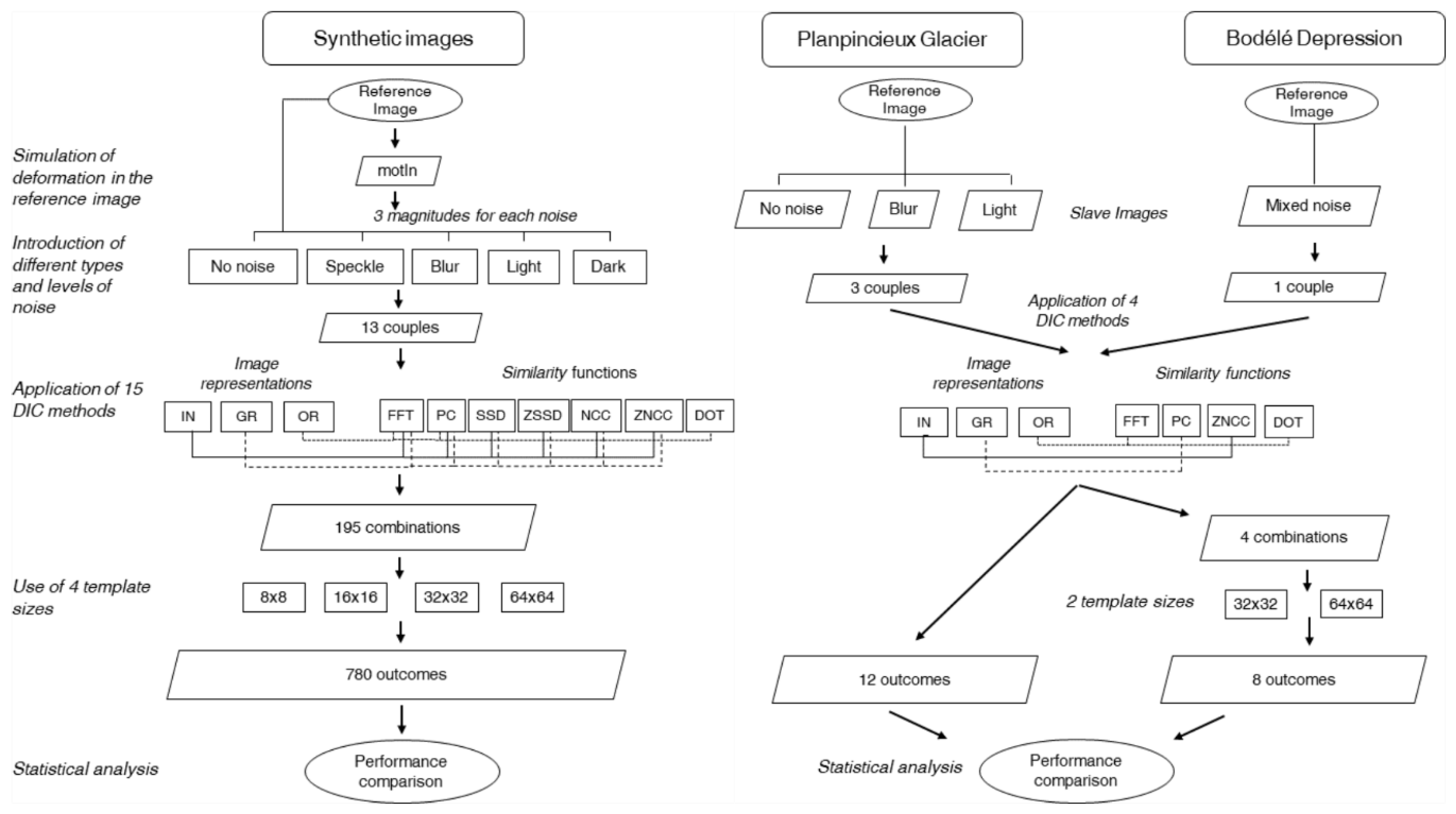
Examples of synthetic images with different types of noise. (A) Reference image; (B) image with displacement and without noise (motIm); (C–F) motIm plus Blur5, LightB, Speckle5 and Dark150 noise respectively. The region of interest (ROI) with simulated displacement is delimited in black. (G) Map of simulated displacement and (H) displacement distribution in the ROI.
Figure 2.
Examples of synthetic images with different types of noise. (A) Reference image; (B) image with displacement and without noise (motIm); (C–F) motIm plus Blur5, LightB, Speckle5 and Dark150 noise respectively. The region of interest (ROI) with simulated displacement is delimited in black. (G) Map of simulated displacement and (H) displacement distribution in the ROI.

Figure 3.
Images of the Planpincieux Glacier: (A) reference image; (B) image acquired in similar illumination conditions; (C) image acquired with different lighting position; (D) image acquired with diffuse illumination and slight blurring. The pairs AB, AC and AD are indicated as PGopt, PGlight and PGblur respectively.

Figure 4.
Sentinel 2B images of the Bodélé Depression. They were acquired in 8 October 2019 and 2 October 2020, respectively. In 2019, one can note the inhomogeneous illumination due to thin clouds and some apparent blurring caused by the strong wind.
Figure 4.
Sentinel 2B images of the Bodélé Depression. They were acquired in 8 October 2019 and 2 October 2020, respectively. In 2019, one can note the inhomogeneous illumination due to thin clouds and some apparent blurring caused by the strong wind.

Figure 5.
Displacement maps, scatterplots of theoretical vs. measured data within the ROI and displacement distributions outside the ROI for every DIC approach using 32 × 32 template size and with Speckle3 noise. The ROI is delimited in black.
Figure 5.
Displacement maps, scatterplots of theoretical vs. measured data within the ROI and displacement distributions outside the ROI for every DIC approach using 32 × 32 template size and with Speckle3 noise. The ROI is delimited in black.

Figure 6.
Displacement maps, scatterplots of theoretical vs. measured data within the ROI and displacement distributions outside the ROI for every DIC approach using 16 × 16 template size and with Blur5 noise. The ROI is delimited in black.
Figure 6.
Displacement maps, scatterplots of theoretical vs. measured data within the ROI and displacement distributions outside the ROI for every DIC approach using 16 × 16 template size and with Blur5 noise. The ROI is delimited in black.

Figure 7.
Outcomes of DIC processing with LightB noise using 16 × 16 template size. (A) mean absolute error with and without considering outliers, black and white bars respectively. (B) Pearson coefficient with and without considering outliers, black and white bars, respectively. (C) Percentage of outliers. (D) Boxplot of the residuals. (E) Difference between the 1st, 2nd and 3rd quartiles, black, grey and white bars, respectively. (F) Standard deviation and mean of the displacement in the stable area (i.e., outside the ROI), white and black bars respectively.

Figure 8.
Outcomes of DIC processing with LightB noise using 64 × 64 template size. (A) mean absolute error with and without considering outliers, black and white bars respectively. (B) Pearson coefficient with and without considering outliers, black and white bars, respectively. (C) Percentage of outliers. (D) Boxplot of the residuals. (E) Difference between the 1st, 2nd and 3rd quartiles, black, grey and white bars, respectively. (F) Standard deviation and mean of the displacement in the stable area (i.e., outside the ROI), white and black bars respectively.

Figure 9.
Displacement values obtained with the images of the Planpincieux Glacier. Rows A–C refer to PGopt, PGlight and PGblur images pairs respectively. Results *1 (A1–C1) are obtained with DOT-OR method, while *2 (A2–C2), *3 (A3–C3) and *4 (A4–C4) are obtained with ZNCC-IN, PC-GR and FFT-OR respectively.

Figure 10.
First row: scatterplot between the outcomes of PGopt vs. those of PGlight. Second row: same as the first row, but PGopt is shown against PGblur. Third row: outcomes of BOD images obtained with the template size of 32 × 32 vs. template of 64 × 64. From left to right, the results have been obtained with DOT-OR, FFT-OR, ZNCC-IN and PC-GR method, respectively.

Figure 11.
Displacement magnitude and direction obtained with images of the Bodélé Depression using 64 × 64 template size. Only the areas with displacement >20 m year−1 are shown. DOT-OR and FFT-OR fail to detect isolated dunes. By contrast, ZNCC-IN spreads the displacement around and it suffers the presence of thin clouds and slight blurring. PC-GR performs well, it shows the best spatial resolution, even though it slightly underestimates the displacement.

Figure 12.
Computational time (in milliseconds) necessary to process one template of various sizes using different correlation functions.
Figure 12.
Computational time (in milliseconds) necessary to process one template of various sizes using different correlation functions.


Table 1.
List of the synthetic images used in this study.
| Noise Type | Noise Type and Magnitude | Acronym |
|---|---|---|
| None | motIm | |
| Blurring | 3 × 3 low-pass mean filter | Blur3 |
| 5 × 5 low-pass mean filter | Blur5 | |
| 7 × 7 low-pass mean filter | Blur7 | |
| Illumination intensity change | linear plan subtraction 0 to 100 | Dark100 |
| linear plan subtraction 0 to 150 | Dark150 | |
| linear plan subtraction 0 to 200 | Dark200 | |
| Lighting source position change | azimuth 10°, elevation 80° | LightA |
| azimuth 30°, elevation 60° | LightB | |
| azimuth 50°, elevation 40° | LightC | |
| Speckling | Variance 0.03 | Speckle3 |
| Variance 0.05 | Speckle5 | |
| Variance 0.07 | Speckle7 |
Table 2.
Specifics of the real images couples.
| Image | Sensor | Image Dimension [px] | Template Size [px] | Dates of Acquisition | Acronym |
|---|---|---|---|---|---|
| Planpincieux Glacier | 27 September 2019 h12 28 September 2019 h12 | PPopt | |||
| Canon EOS 700D | 5184 × 3456 | 64 × 64 | 27 September 2019 h12 28 September 2019 h08 | PPlight | |
| 27 September 2019 h12 27 September 2019 h19 | PPblur | ||||
| Bodélé Depression | Sentinel 2B | 2000 × 2000 | 32 × 32 64 × 64 | 8 October 2019 2 October 2020 | BOD |
Table 3.
Performance score based on the qualitative analysis of the results. The rightmost column reports the total score obtained for every template size separately (i.e., 8 × 8/16 × 16/32 × 32/64 × 64).
Table 3.
Performance score based on the qualitative analysis of the results. The rightmost column reports the total score obtained for every template size separately (i.e., 8 × 8/16 × 16/32 × 32/64 × 64).
| motIm | Blur3 | Blur5 | Blur7 | Dark 100 | Dark 150 | Dark 200 | LightA | LightB | LightC | Speckle 3 | Speckle 5 | Speckle 7 | Score | |
|---|---|---|---|---|---|---|---|---|---|---|---|---|---|---|
| FFT-GR | o+++ | -+++ | --oo | ---- | o+++ | -+++ | o+++ | o+++ | -+++ | --oo | --o+ | --oo | ---- | −9/1/5/6 |
| PC-GR | o++o | -++o | ---- | ---- | o++o | o++o | o++o | o++o | -o+o | --oo | --oo | ---o | ---- | −8/−1/3/−3 |
| SSD-GR | +++o | o++o | ---o | ---- | +++o | +++o | +++o | ++o+ | --oo | ---- | ---- | ---- | ---- | −2/−1/−1/−4 |
| ZSSD-GR | ++++ | ++++ | --+o | ---- | ++++ | ++++ | ++++ | ++++ | ooo+ | ---o | --oo | ---o | ---- | 0/0/3/5 |
| NCC-GR | ++++ | ++++ | --oo | ---- | ++++ | ++++ | ++++ | ++++ | o+++ | --oo | -oo+ | --o+ | ---o | 0/2/5/8 |
| ZNCC-GR | ++++ | ++++ | o-oo | ---- | ++++ | ++++ | ++++ | ++++ | oo++ | --oo | -oo+ | --oo | ---o | 1/1/5/7 |
| FFT-IN | o+++ | o++o | -ooo | -o-- | o+++ | o+++ | o+++ | o+++ | oooo | ---- | -+++ | -+++ | -o++ | −6/7/7/6 |
| PC-IN | o++o | -ooo | ---- | ---- | o++o | o++o | o++o | o++o | -++o | ---o | -o+o | -o+o | --o+ | −8/2/5/1 |
| SSD-IN | +++o | +++o | ++oo | oooo | ---- | ---- | ---- | o++o | ---- | ---- | o++o | oo+o | oo+o | −2/0/1/5 |
| ZSSD-IN | ++++ | +++o | +++o | -ooo | ++++ | ++++ | +++o | ++++ | oooo | ---- | o+++ | -o++ | -o++ | 3/7/9/6 |
| NCC-IN | ++++ | +++o | +++o | -+oo | ++++ | ---o | ---- | ++++ | oo+o | ---- | o+++ | oo++ | -o++ | 0/4/6/4 |
| ZNCC-IN | ++++ | +++o | +++o | -ooo | ++++ | ++++ | +++o | ++++ | oo+o | ---- | o+++ | o+++ | oo++ | 5/8/10/6 |
| FFT-OR | o+++ | o+++ | -ooo | ---- | o+++ | o+++ | o+++ | o+++ | o+++ | ---o | -o++ | -o++ | --++ | −6/4/8/9 |
| PC-OR | o+++ | -o++ | ---- | ---- | o+++ | o+++ | o+++ | o+++ | -++o | --oo | --++ | --o+ | --o+ | −8/0/6/7 |
| DOT-OR | ++++ | ++++ | +o+o | --o- | ++++ | ++++ | ++++ | ++++ | ++++ | oooo | o+++ | oo++ | -o++ | 6/7/11/9 |
Publisher’s Note: MDPI stays neutral with regard to jurisdictional claims in published maps and institutional affiliations. |
© 2021 by the authors. Licensee MDPI, Basel, Switzerland. This article is an open access article distributed under the terms and conditions of the Creative Commons Attribution (CC BY) license (http://creativecommons.org/licenses/by/4.0/).
Share and Cite
MDPI and ACS Style
Dematteis, N.; Giordan, D. Comparison of Digital Image Correlation Methods and the Impact of Noise in Geoscience Applications. Remote Sens. 2021, 13, 327. https://0-doi-org.brum.beds.ac.uk/10.3390/rs13020327
AMA Style
Dematteis N, Giordan D. Comparison of Digital Image Correlation Methods and the Impact of Noise in Geoscience Applications. Remote Sensing. 2021; 13(2):327. https://0-doi-org.brum.beds.ac.uk/10.3390/rs13020327
Chicago/Turabian StyleDematteis, Niccolò, and Daniele Giordan. 2021. "Comparison of Digital Image Correlation Methods and the Impact of Noise in Geoscience Applications" Remote Sensing 13, no. 2: 327. https://0-doi-org.brum.beds.ac.uk/10.3390/rs13020327
Note that from the first issue of 2016, this journal uses article numbers instead of page numbers. See further details here.