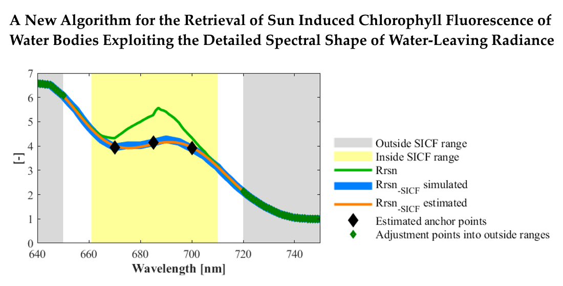
A New Algorithm for the Retrieval of Sun Induced Chlorophyll Fluorescence of Water Bodies Exploiting the Detailed Spectral Shape of Water-Leaving Radiance

Abstract

Sun induced chlorophyll fluorescence (SICF) emitted by phytoplankton provides considerable insights into the vital role of the carbon productivity of the earth’s aquatic ecosystems. However, the SICF signal leaving a water body is highly affected by the high spectral variability of its optically active constituents. To disentangle the SICF emission from the water-leaving radiance, a new high spectral resolution retrieval algorithm is presented, which significantly improves the fluorescence line height (FLH) method commonly used so far. The proposed algorithm retrieves the reflectance without SICF contribution by the extrapolation of the reflectance from the adjacent regions. Then, the SICF emission curve is obtained as the difference of the reflectance with SICF, the one actually obtained by any remote sensor (apparent reflectance), and the reflectance without SICF, the one estimated by the algorithm (true reflectance). The algorithm first normalizes the reflectance spectrum at 780 nm, following the similarity index approximation, to minimize the variability due to other optically active constituents different from chlorophyll. Then, the true reflectance is estimated empirically from the normalized reflectance at three wavelengths using a machine learning regression algorithm (MLRA) and a cubic spline fitting adjustment. Two large reflectance databases, representing a wide range of coastal and ocean water components and scattering conditions, were independently simulated with the radiative transfer model HydroLight and used for training and validation of the MLRA fitting strategy. The best results for the high spectral resolution SICF retrieval were obtained using support vector regression, with relative errors lower than 2% for the SICF peak value in 81% of the samples. This represents a significant improvement with respect to the classic FLH algorithm, applied for OLCI bands, for which the relative errors were higher than 40% in 59% of the samples.

1. Introduction

Phytoplankton is the base of the trophic pyramid in aquatic ecosystems, using solar energy for energy fixation in carbon compounds, and playing a key role in the earth’s carbon cycle. The monitoring of chlorophyll-a (Chla) fluorescence emitted by phytoplankton is one of the most used methods to understand the state of aquatic ecosystems [1,2,3]. When the Chla molecules present in phytoplankton are excited by absorbed light, the excitation energy can either (1) be used in the photosynthetic chain, (2) be dissipated as heat, or (3) be emitted as Chla fluorescence in the 650–800 nm region and measurable as a contribution to the peak within the 660–750 nm region on the water-leaving radiance or reflectance of water bodies [4]. As shown by Gower and Maritorena [5,6], the sun induced chlorophyll fluorescence (SICF) emission curve in natural waters can be approximated by a Gaussian function with a maximum at ∼685 nm and a full width at half maximum (FWHM) of 25 nm. In addition to SICF, the fluorescence quantum yield (ϕ SICF) is defined as the ratio of the number of photons emitted to the number of photons absorbed by the Chla.

The measurement of SICF, and its quantum yield of photosynthetic organisms in natural waters, adds information that can be interpreted in terms of phytoplankton physiology [1,7,8] and species composition [9]. The SICF signal has been used to estimate the phytoplankton’s biomass [1,10,11,12], photosynthetic activity, and primary productivity [13,14]. The use of optical remote sensing data in the visible–near-infra-red (VNIR) spectral range (400–800 nm) for the estimation of SICF and ϕ has demonstrated its potential to describe the spatial and temporal variability of the physiological status of marine phytoplankton, linked to nutrient limitation [10,15].

The fluorescence line height (FLH) algorithm, developed to retrieve SICF [16], estimates the height of the red fluorescence peak by using the water-leaving radiance ($L_w$) or remote-sensing reflectance ($Rrs$, defined as the ratio of $L_w$ and $E_d$, the sun irradiance arriving at the water surface, called here apparent reflectance) at three wavelengths, one which is centered on the SICF peak and two others that are used to define a baseline below the SICF peak. The FLH algorithm is routinely implemented for global ocean image processing using MODIS and MERIS/OLCI data [17,18,19]. The accuracy in the estimation of the actual fluorescence peak height (centered around 685 nm) depends on the position of the three bands used in the FLH [18,20] and the signal-to-noise of the sensor used. It has been shown that the SICF signal retrieved by MODIS (peak band at 677 nm, with 11 nm of FWHM) responds to only 57% of SICF signal, while MERIS/OLCI (peak band at 681.25 nm, with 7.5 nm of FWHM) reaches 78% of the SICF signal [21].

The main difficulty in retrieving SICF is the variability in the concentration and optical properties of the optically active constituents (OACs) of water bodies, producing a large variability in the shape of $Rrs$, especially in the visible wavelengths. The main OACs are (1) pure water itself; (2) phytoplankton, containing a large number of different pigments, the most abundant being Chla, which is present in all phytoplankton cells; (3) colored dissolved organic matter (CDOM); and (4) non-algal particles (NAP) composed of organic particles (e.g., bacteria, protists, zooplankton, detrital organic matter) and suspended inorganic particles. Hence, the detection of SICF by remote sensors is mainly affected, within the emission region, by the absorption properties of water and phytoplankton, plus the particle scattering (from both phytoplankton cells and NAP). The combination of these three effects produces a reflectance peak in the SICF region that overlaps with the actual emission peak at low Chla concentration ([Chla]) and could become dominant with increasing [Chla] and/or NAP concentration [22,23,24,25].

Further difficulties to obtain SICF accurately from the reflected radiance signal are the strong effects of the atmospheric compounds, selectively attenuating the signal. The earth’s atmosphere is composed mainly of molecular gases (i.e., O₂, O₃, CO₂, water vapor) and particles suspended in the gases (aerosols). The scattering and absorption produced by these atmospheric compounds strongly affects the signal detected by any remote sensor, especially for signals leaving from water surfaces, where the contribution of $L_w$ in general is much lower than the total radiance arriving at any remote sensor. In the spectral SICF range, the signal is strongly affected by the water vapor and O₂ absorptions. In addition to the standard atmospheric effects to be compensated for water targets, the case of fluorescence emission requires that the in-filling of the O2-B band due to fluorescence emission should be taken into account as part of the atmospheric correction process, but this is not analyzed in this paper.

As introduced above, the performance of the FLH algorithm applied on $Rrs$ is affected by the overlap between SICF and the reflectance peak in the same spectral region in water bodies with high [Chla] [4], producing a “shoulder” in the 660–750 nm region. The shape of this reflectance “shoulder” is due to the combined absorption features of phytoplankton and water, while its magnitude is due to the particle scattering. The combined result of these effects determines that, in productive waters, the linear baseline assumption no longer holds, since the fluorescence peak adds to a curved reflectance beneath. Therefore, the FLH calculated with the simple baseline approach leads to inaccurate SICF retrievals [26].

The use of a high spectral resolution sensor providing narrower bands than MODIS or MERIS/OLCI to detect SICF in water allows one to detect a more accurate contribution of SICF from a higher detailed shape of the water-leaving radiance, avoiding the atmospheric O₂-B (687 nm) absorption band. The ongoing satellite missions that include sensors with higher spectral and radiometric resolutions (i.e., FLEX [27], CHIME [28]), increase the possibilities of retrieving a more accurate SICF peak height and width and, therefore, a more accurate total emission. Hence, the aim of this work is to define an algorithm able to separate the SICF emission signal from the peak produced by the combined effects of water and phytoplankton absorption and scattering by exploiting the detailed spectral shape of water-leaving radiance and considering the spectral variability of water.

The measurement of SICF in natural waters is, however, challenging. There are no standard instruments or protocols and very few actual measurements. The fluorescence measurements routinely done in the ocean, obtained with artificial light sources, can be considered as proxies of the SICF, but not its actual measurement in W m⁻² sr⁻¹. Since in situ SICF data were not available, the methodology proposed in this manuscript was based entirely on simulated data. To ensure the maximum representativeness of the results, a very comprehensive radiative transfer model was used, and the ranges of OAC and the inherent optical properties were chosen to represent the widest variability of ocean and coastal waters.

2. Background and Definitions

Throughout this work, two different definitions of the remote sensing reflectance are used. The $Rrs$ widely used in ocean optics is called here “apparent” reflectance, because the water-leaving radiance includes the emitted fluorescence contribution (SICF). Further, the ”true” reflectance is defined as the water-leaving remote sensing reflectance without the SICF contribution ($Rr{s}_{-SICF}$) (Equations (1) and (2)):

$$L_{w-SICF}\left(\lambda \right) = L_w\left(\lambda \right)-SICF\left(\lambda \right) \left[\mathrm{W}·{\mathrm{m}}^{-2}·{\mathrm{sr}}^{-1}·{\mathrm{nm}}^{-1}\right]$$

(1)

$$Rr{s}_{-SICF}\left(\lambda \right) = \frac{L_{w-SICF}\left(\lambda \right) }{E_d\left(\lambda \right)} \left[s{r}^{-1}\right]$$

(2)

where $E_d\left(\lambda \right)$ is the downwelling plane irradiance arriving at the water surface (W·m⁻²·nm⁻¹). The issue with the definitions of “apparent” reflectance and “true” reflectance also comes from the consideration of the bidirectional reflectance distribution function (BRDF), and from adjacency effects, which are not negligible for coastal areas and inland waters. While a full consideration of these effects is outside the scope of this paper, they must be taken into account during the atmospheric correction procedure.

In water bodies, the upwelling radiance is the result of (1) scattering and absorption from particles and dissolved substances, and (2) emission contribution from SICF. Therefore, $Rrs$ corresponds to $Rr{s}_{-SICF}$ plus the SICF contribution, with $Rrs$ being the reflectance observed by the sensor and $Rr{s}_{-SICF}$ the unknown true reflectance component. It is important to recall that outside the fluorescence emission region (i.e., <660 nm and >750 nm) both reflectances are identical (Figure 1).

To improve the SICF retrieval method for water bodies, we propose to further consider the spectral variability of water bodies due to the OAC of water, based on their spectral modelling. Moreover, the advantage is that the SICF spectral range is only slightly affected by the OAC. While the variability in the shape of $Rrs$ in the visible wavelengths is high, the shape of the $Rr{s}_{-SICF}$ spectrum in the near-infrared (NIR) spectral range (700–900 nm) is largely determined by pure water absorption and thus is almost invariant [29].

Next, the modeling of the inherent optical properties (absorption and scattering) performed in this work is described.

2.1. Absorption

The total absorption coefficient ($a\left(\lambda \right)$) can be expressed as the sum of the absorption coefficients of each OAC:

$$a\left(\lambda \right) = a_w\left(\lambda \right) + a_{CDOM}\left(\lambda \right) + a_{phy}\left(\lambda \right) + a_{NAP}\left(\lambda \right) \left[m^{-1}\right]$$

(3)

The absorption by pure water $a_w\left(\lambda \right)$ corresponds to the absorption described by Pope and Fry [30].

The absorption by CDOM $a_{CDOM}\left(\lambda \right)$ is modeled as [31]

$$a_{CDOM}(\lambda )=a_{CDOM}\left({\lambda }_o\right)e^{-0.014\left(\lambda -\lambda o\right) }{}_{ }$$

(4)

where $a_{CDOM}\left({\lambda }_o\right)$ is the absorption coefficient at ${\lambda }_o$ = 440 nm.

The absorption by phytoplankton $a_{phy}\left(\lambda \right)$ is given by [32] as follows:

$$a_{phy}(\lambda )=0.06a_c^{*}{}_{ }\left(\lambda \right){\left[Chla\right]}^{0.65 }{}_{ } \left[m^{-1}\right]$$

(5)

where [Chla] is supplied in mg·m⁻³, and $a_c^{*}{}_{ }\left(\lambda \right)$ is the chlorophyll-specific absorption coefficient in m²·mg⁻¹ representative of marine phytoplankton [33,34].

In the case of the absorption by NAP, $a_{NAP}\left(\lambda \right)$, the next expression is used [35]:

$$a_{NAP}(\lambda )=a^{*}{}_{ }\left(\lambda \right){\left[NAP\right]}^{ }{}_{ } \left[m^{-1}\right]$$

(6)

where [NAP] is supplied in g·m⁻³, and a^∗(λ) is the mineral particle-specific absorption coefficient in m²·g⁻¹.

2.2. Scattering

The angular distribution of light scattered by a particle in a direction $\psi$ at a wavelength $\lambda$ is defined as the volume scattering function ($\beta \left(\psi ,\lambda \right)$). The total spectral scattering coefficient $\left(b\left(\lambda \right)\right)$ is the total magnitude of the scattered light, which corresponds to the integral of $\beta \left(\psi ,\lambda \right)$ over all angles 4π. The phase function ($\tilde{\beta }\left(\psi ,\lambda \right)$) corresponds to $\beta \left(\psi ,\lambda \right)$ normalized to $b\left(\lambda \right)$, providing the shape of the $\beta \left(\psi ,\lambda \right)$ regardless of the intensity of the scattered light. The total backscattering coefficient ($b_b\left(\lambda \right)$) is the total light scattered in the backward direction, and the backscattered fraction with respect to total scattering ($\tilde{b}\left(\lambda \right)$) is defined as the ratio between $b_b\left(\lambda \right)$ and $b\left(\lambda \right)$ [32].

Regarding scattering modeling, it only considers the scattering coming from phytoplankton and NAP. The contribution of CDOM in the total scattering ($b\left(\lambda \right)$) is considered to be negligible [31].

As the scattering of phytoplankton and NAP depends on the size, structure, distribution, and composition of the particles, it is not easy to model the integral effects. Hence, a realistic approximation given by the spectral beam attenuation coefficient of particles $c_p\left(\lambda \right)$ is used to model $b\left(\lambda \right)$ for phytoplankton and NAP [36]:

$$c_p\left(\lambda \right) = c_{wp}\left({\lambda }_o\right){\left(\frac{\lambda }{{\lambda }_o}\right)}^{-n} \left[m^{-1}\right]$$

(7)

where ${\lambda }_o$ is a nominal scaling wavelength, and n can have values from 0 to 1, depending on the size distribution (large particles have a small n; small particles have a large n).

Therefore, b(λ) is calculated as the difference between $c_p\left(\lambda \right)$ and $a\left(\lambda \right)$ according to [37] as follows:

$$b\left(\lambda \right) = c_p\left(\lambda \right)- a\left(\lambda \right) \left[m^{-1}\right]$$

(8)

2.3. Similarity Index

$Rrs$ is related to the total spectral absorption coefficient ($a\left(\lambda \right)$) and total backscattering coefficient ($b_b\left(\lambda \right)$) [29]:

$$Rrs\left(\lambda \right) =\kappa \frac{b_b\left(\lambda \right)}{a\left(\lambda \right) + b_b\left(\lambda \right)}$$

(9)

where κ is a coefficient that depends on the illumination conditions. In the NIR, it is assumed that the total absorption coefficient ($a\left(\lambda \right)$) is dominated by $a_w\left(\lambda \right)$, since $a_{CDOM}\left(\lambda \right)$ is negligible, and $a_{phy}\left(\lambda \right)$ and $a_{NAP}\left(\lambda \right)$ are very low in this region. It is also assumed that $b_b\left(\lambda \right)$ is almost spectrally flat for wavelengths in the NIR (${\lambda }_{NIR}$), and therefore Equation (9) can be redefined as [29,38]

$$Rrs\left({\lambda }_{NIR}\right) =\kappa \frac{b_b\left({\lambda }_{NIR}\right)}{a_w\left({\lambda }_{NIR}\right)}$$

(10)

The normalized $Rrs \left(Rrsn\right)$, derived from the similarity index concept applied to the NIR region, is defined by dividing the reflectance by its value at 780 nm [29], a wavelength that is only affected by pure water absorption. The concept of similarity index is therefore useful since it allows $Rrsn$ in the red-NIR region to be obtained, where other OACs except for pure water can be neglected. Therefore, it provides a first guess of the shape of the $Rr{s}_{-SICF}$ in the region where the SICF emission peak occurs. The calculation of $Rrsn$ is the first concept of the strategy underlying the SICF retrieval algorithm presented in this paper.

In the entire visible region, however, the normalized remote sensing reflectance without SICF contribution ($Rrs{n}_{-SICF}\left(\lambda \right)$) deviates from the ideal similarity index shape due to the non-negligible absorption and scattering of the different OACs. If a comprehensive simulation of the variability of OACs and illumination and surface conditions is performed in water bodies, the deviations of $Rr{s}_{-SICF}\left(\lambda \right)$ within the SICF region could be empirically estimated from a database of $Rrs\left(\lambda \right)$ outside that region. This is the second concept underlying the algorithm strategy presented here.

3. Materials and Methods

To build the simulated databases, the radiative transfer model (RTM) HydroLight (HL) [32] was used. HL is an RTM that computes radiance distributions and derived quantities (irradiances, reflectances, fluorescence, etc.) for water bodies. The spectral radiance distribution is computed as a function of depth, direction, and wavelength within the water. The upwelling radiance just above the sea surface includes both the water-leaving radiance ($L_w\left(\lambda \right)$) and that part of the incident direct and diffuse sky radiance that is reflected upward by the wind-blown sea surface [32]. HL employs mathematically sophisticated invariant embedding techniques to solve the radiative transfer equation [32]. It includes the effects of SICF assuming that Chla always fluoresces in the band centered at 685 nm, regardless of whether it is excited by light at near ultraviolet, blue, green, or even red wavelengths [32]. To calculate the amount of emitted SICF, HL uses the computed scalar irradiance, the absorption by Chla, and various assumptions about the fluorescence efficiency and the wavelength redistribution function approximated by a Gaussian, with 685 nm the mean wavelength and 10.6 nm the standard deviation of the Gaussian, which corresponds to a value of 25 nm for the FWHM of the emission band [32,35].

3.1. Training Database of Remote Sensing Reflectance and Normalized Remote Sensing Reflectance without SICF Contribution ($Rr{s}_{-SICF},Rrs{n}_{-SICF}$)

To train the retrieval algorithm for true reflectance, which is the base for the SICF retrieval described in this paper, a large database of “true” remote sensing reflectances was constructed with HL. This database consisted of 7200 simulations of $Rr{s}_{-SICF}$ with 1 nm of spectral sampling, obtained from all combinations of the input variables given in

Table 1. Variation of optically active constituent (OAC) parameters used in HL to simulate the 7200 spectra of $Rr{s}_{-SICF}$. The range of values for each parameter was taken according to values known in the literature (see column Reference).

Parameter	Units	Value	Reference
$a_{CDOM}\left(\lambda o\right)$	m−1	0.00, 0.01, 0.20, 0.50, 2.00, 5.00	[41]
[Chla]	mg·m−3	0.01, 0.02, 0.05, 0.10, 0.25, 0.50, 0.75, 1.00, 1.50, 2.00, 5.0, 10.00, 15.00, 20.00, 30.00	[41]
m	-	0, 0.5, 1, 1.5	[42,43]
${\tilde{b}}_p\left({\lambda }_0\right)$	-	0.0001, 0.001, 0.01, 0.1,0.4	[39]
SZA	degrees	0, 30, 50, 70	-

, comprising high variability in water components (Chla and CDOM), as well as including the variability of the scattering coefficient due to the particles’ shapes and sizes (by varying the parameters ${\tilde{b}}_p\left({\lambda }_0\right)$ and m in Equation (11) [35]) and illumination conditions (solar zenith angle (SZA)).

The backscattered fraction with respect to total scattering from particles $({\tilde{b}}_p(\lambda ))$ is defined as follows [35]:

$${\tilde{b}}_p\left(\lambda \right) = {\tilde{b}}_p\left({\lambda }_0\right){\left(\frac{{\lambda }_0}{\lambda }\right)}^m$$

(11)

where ${\lambda }_0$ = 550 nm, and ${\tilde{b}}_p\left({\lambda }_0\right)$ and m are values supplied by the user. Accordingly, HL generates a Fournier–Forand phase function using ${\tilde{b}}_p\left(\lambda \right)$ [39]. Hereby, the simulated phase functions are a combination of “small” and “large” particle phase functions, depending on the ${\tilde{b}}_p\left({\lambda }_0\right)$ and m values.

This database is intended to be a representation of the typical spectral behavior of $Rr{s}_{-SICF}$ in coastal and oceanic waters. Due to the effect of high scattering by NAP over the SICF signal [23,40], NAP was not included in this simulation.

The simulated database spectra are shown in Figure 2 (left) together with the calculated $Rrs{n}_{-SICF}$ for each simulation Figure 2 (right). A high variability of $Rrs{n}_{-SICF}$ between 640–720 nm and a very low variability for wavelengths higher than 720 nm is observed, in accordance with the similarity index concept.

3.2. Validation Database of Remote Sensing Reflectance and Normalized Remote Sensing Reflectance with and without SICF Contribution ($Rrs,Rrsn,Rr{s}_{-SICF},Rrs{n}_{-SICF}$)

To validate the SICF retrieval algorithm, a database of 400 random spectra was simulated, here called the validation database (VDB). The VDB was simulated with the HL chlorophyll fluorescence option enabled (considered here as “observed data”) to simulate water-leaving remote sensing reflectance ($Rrs$) and disabled (considered here as “reference data”) to simulate water-leaving remote sensing reflectance without SICF contribution ($Rr{s}_{-SICF}$) data. The VDB includes the simulation of NAP according to the values in

Table 2. Variation of parameters to simulate the validation database (VDB).

Parameter	Units	Range of Values/Classes	Reference
$a_{CDOM}\left(\lambda o\right)$	m−1	0.001–9.75	[41]
[Chla]	mg·m−3	0.009–30	[41]
[NAP]	g·m−3	0–13.5	[23,40]
Type of NAP	-	Brown earth, yellow clay, calcareous sand, red clay, mixed Bukata	[44,45]
Discrete phase function	-	avgpart, isotrop, Case Small, Case Large, Petzold clear, coastal and harbor, FFbb001 to FFbb500 (for 0.01% to 50% backscatter fraction)	[32,47,48]
ϕSICF		0.001–0.02	[25,46]
SZA	degrees	1–79

.

Unlike the training database, the ${\tilde{b}}_{ }\left(\lambda \right)$ modeling for the simulation of the VDB by HL has been performed by selecting a discretized phase function available in the HL library. These discretized phase functions used by HL are the quad-averaged and Fourier-decomposed phase functions computed as described in [32]. This ${\tilde{b}}_{ }\left(\lambda \right)$ modeling is made for both Chla and NAP. Several mass-specific absorption spectra for mineral particles are included in the HL library and are available for brown earth, calcareous sand, yellow clay, red clay [44], and Bukata mix [45]. The variability of SICF is simulated, variating the fluorescence quantum yield (ϕSICF) parameter in HL between 0.001 and 0.02 according to [25,46]. The considered variable parameters in VDB are described in Table 2.

In Figure 3, the variability of the SICF curve, obtained in the simulations of the VDB, is shown.

3.3. Regression Methods

Machine learning regression algorithm (MLRA) methods were used to estimate $Rrs{n}_{-SICF}\left(\lambda \right).$ MLRA methods have become one of the key tools used in many applications, such as signal and image processing and computer science. They are based on the concept that an algorithm can be trained to learn from data without being explicitly programmed to perform specific tasks. MLRA methods have been used in many remote sensing studies as powerful tools for the inversion of RTMs [49,50]. MLRA methods are robust, and in most cases they are very fast to apply once trained and are able to manage the nonlinear relationship between the output/input data. However, the large majority of methods do not have multi-output capability, and superior accuracies are achieved when MLRA methods are trained per variable, as then the algorithm is more optimized [51,52].

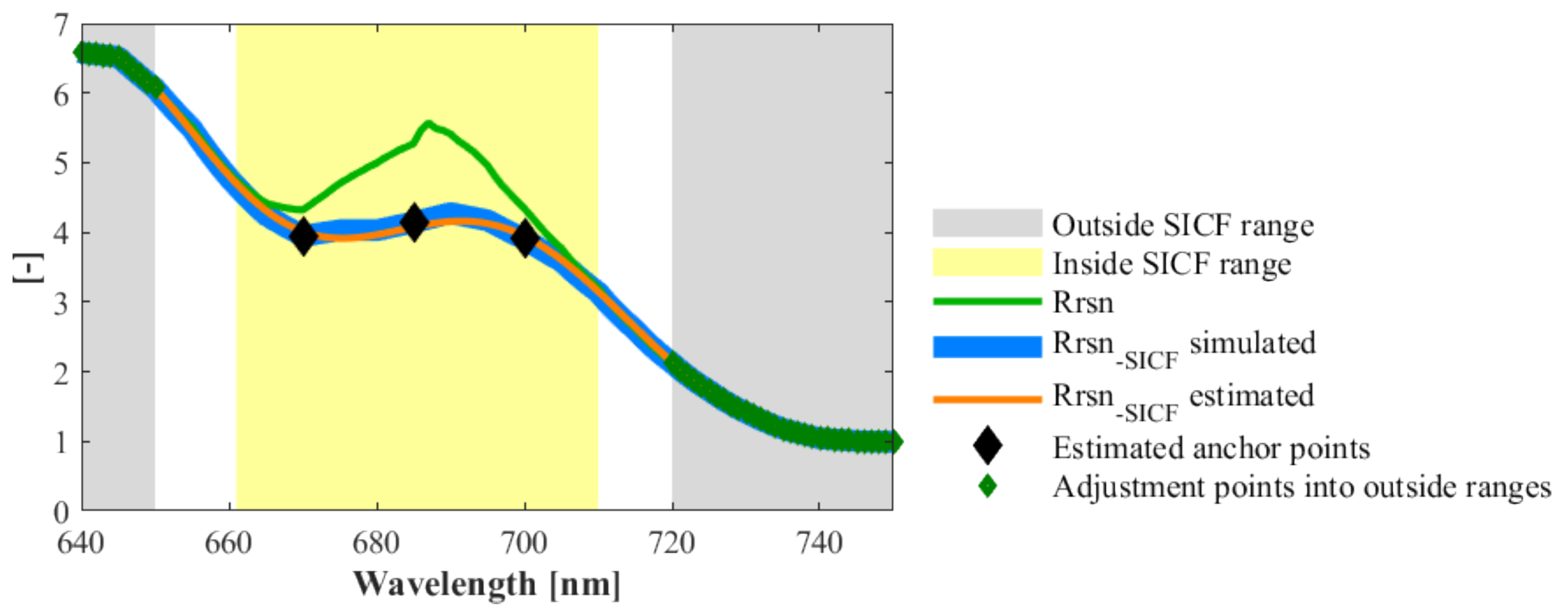
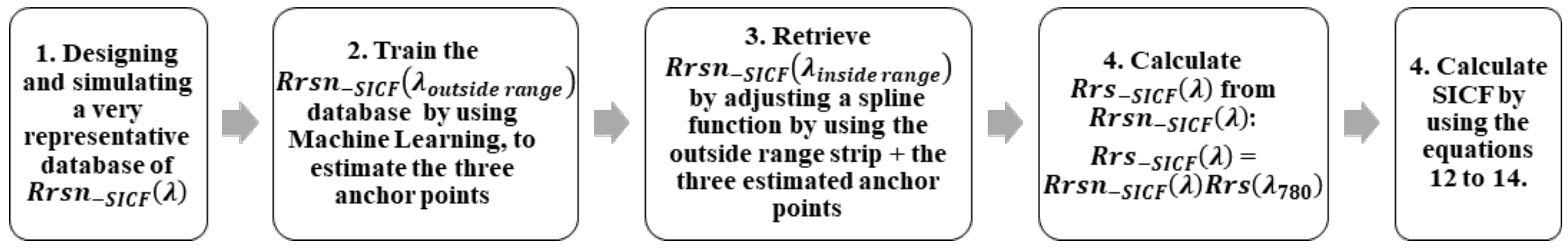
4. Algorithm Development

In this work, the retrieval of SICF was based on the modeling of $Rrs{n}_{-SICF}\left(\lambda \right)$ (normalized remote-sensing reflectance without SICF contribution), which is key in the modeling of the major unknown $Rr{s}_{-SICF}\left(\lambda \right)$, to resolve the SICF contribution from the water-leaving radiance according the following steps:

$$L_w\left(\lambda \right) = Rrs\left(\lambda \right)E_d\left(\lambda \right)$$

(12)

$$L_{w-SICF}\left(\lambda \right) = Rr{s}_{-SICF}\left(\lambda \right)E_d\left(\lambda \right)$$

(13)

$$SICF(\lambda )=L_w\left(\lambda \right)-L_{w-SICF}\left(\lambda \right)$$

(14)

Assuming that after atmospheric correction of remotely sensed images (or from in situ measurements), $Rrs\left(\lambda \right)$ and $E_d\left(\lambda \right)$ can be obtained with an acceptable error, the remaining variable to be retrieved is $Rr{s}_{-SICF}\left(\lambda \right)$, and this is the objective of the algorithm described in this paper.

The normalization of $Rrs$ at 780 nm ($Rrsn\left(\lambda \right)$) in the NIR region reduces the spectral variability in the red–NIR spectral range and thus facilitates finding a better mathematical adjustment for the estimation of $Rrs{n}_{-SICF}\left(\lambda \right)$, the major unknown. The proposed methodology to find such adjustment consists of the following steps: (1) analyzing normalized remote-sensing reflectance at 780 nm without SICF contribution ($Rrs{n}_{-SICF}\left(\lambda \right)$) behavior based on the representative database of $Rr{s}_{-SICF}\left(\lambda \right)$, simulated in Section 3.1; (2) obtaining an algorithm from the analysis done in the previous step, allowing the estimation of $Rrs{n}_{-SICF}\left(\lambda \right)$ within the SICF spectral range from $Rrsn\left(\lambda \right)$, assuming that $Rrs{n}_{-SICF}\left(\lambda \right)$ within the SICF spectral range is unknown, and $Rrsn\left(\lambda \right)$ and $Rrs{n}_{-SICF}\left(\lambda \right)$ are equal outside of the SICF range; (3) training different MLRA methods to estimate $Rrs{n}_{-SICF}\left(\lambda \right)$ using the large database simulated in step 1; and (4) using the simulated random database containing $Rrs{n}_{-SICF}\left(\lambda \right)$ and $Rrsn\left(\lambda \right)$ described in Section 3.2 to validate the obtained algorithm.

Estimation of Normalized Remote-Sensing Reflectance without SICF Contribution ($Rrs{n}_{-SICF}(\lambda )$) from Normalized Remote-Sensing Reflectance ($Rrsn$)

It is assumed that $Rrsn\left(\lambda \right)$ and $Rrs{n}_{-SICF}\left(\lambda \right)$ have the same spectral shape in the outer ranges 640–650 nm and 720–750 nm due to the fact that these ranges are, respectively, not or minimally affected by the SICF contribution (Figure 3). Hence, the estimation of $Rrs{n}_{-SICF}\left(\lambda \right)$ from $Rrsn$ is based on this assumption of shape stability in the outer SICF regions [32]. The ranges outside of the SICF signal (from 640 to 650 nm and from 720 to 750 nm) are called “outside range 1” and “outside range 2”, respectively, and the range inside the SICF signal (from 661 to 710 nm) is hereafter called the “inside range”. The “outside range 2” was defined to 750 nm to avoid the O₂-A absorption band (760 nm) (Figure 4).

Estimation of $Rrs{n}_{-SICF}\left(\lambda \right)$ from $Rrsn\left(\lambda \right)$ was performed using MLRA methods taking all the bands in the “outside ranges” as inputs to calculate the reflectance in the inside region. Due to the multi-output limitations in the MLRA methods, only three anchor points located within the “inside range” were defined for the estimation. These three “inside range” anchor points of $Rrs{n}_{-SICF}\left(\lambda \right)$ were chosen evenly spaced within the SICF emission region at 670, 685, and 700 nm (Figure 4).

Once these anchor points were estimated, the $Rrs{n}_{-SICF}\left(\lambda \right)$ spectra in the range between 640 and 750 nm were re-constructed by a cubic spline fitting using the outside ranges, as shown in the Figure 4.

Once $Rrs{n}_{-SICF}\left(\lambda \right)$ was estimated, $Rr{s}_{-SICF}\left(\lambda \right)$ was obtained by multiplying $Rrs{n}_{-SICF}\left(\lambda \right)$ by $Rrs\left({\lambda }_{780}\right)$.

Four MLRA methods were used to train the estimation of the three anchor points: kernel ridge regression (KRR) [53,54], Gaussian process regression (GPR) [55], support vector regression (SVR) [56], and neural networks (NNs) [54,57].

The steps followed to obtain SICF from $Rrs{n}_{-SICF}\left(\lambda \right)$ are summarized in Figure 5.

5. Results and Discussion

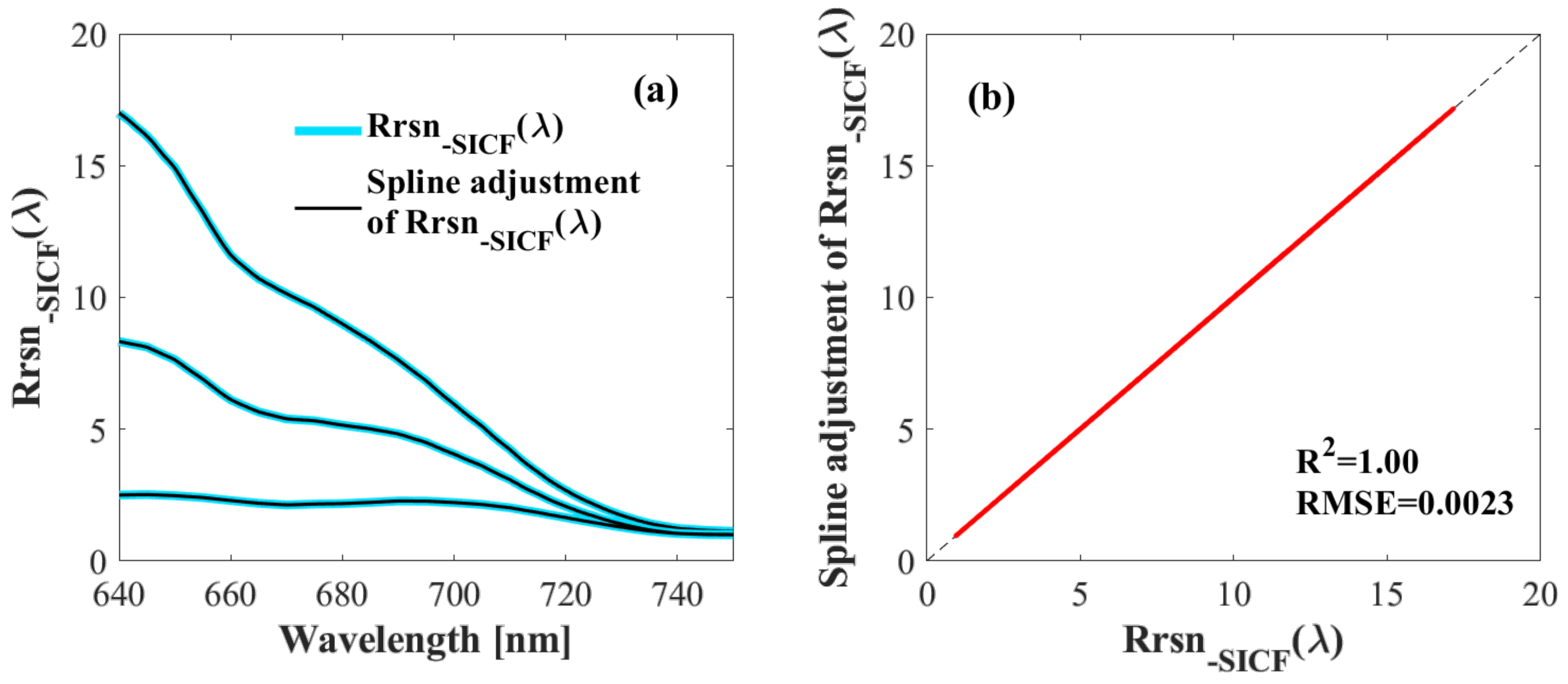
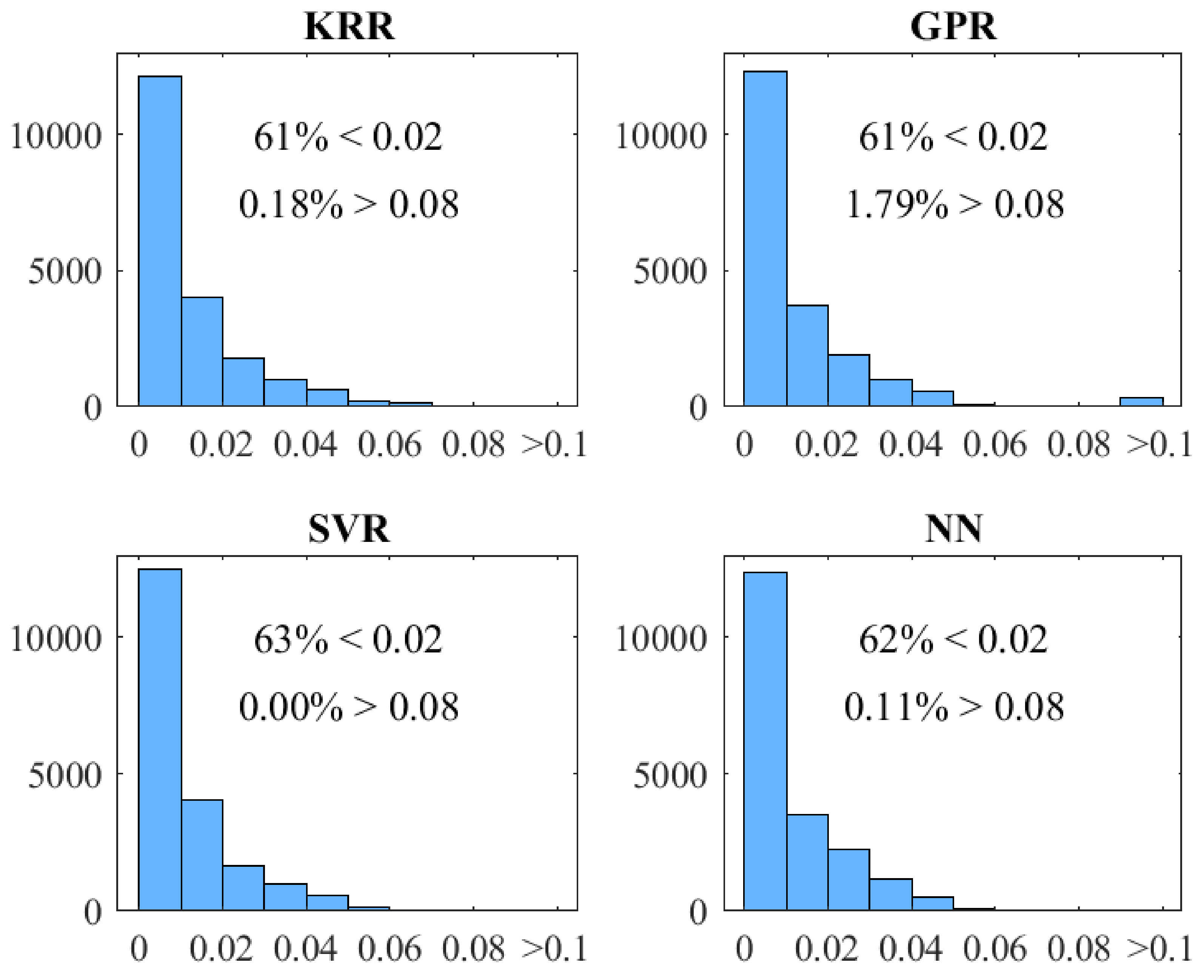
5.1. Fitting of Normalized Remote-Sensing Reflectance without SICF Contribution ($Rrs{n}_{-SICF}(\lambda )$)

The performance of the cubic spline fitting method was assessed for the 7200 $Rrs{n}_{-SICF}\left(\lambda \right)$ spectra of the calibration database in the spectral range between 640 and 750 nm. Each of the $Rrs{n}_{-SICF}\left(\lambda \right)$ spectra was fitted using a cubic spline function, and then this fitting was compared to the simulated $Rrs{n}_{-SICF}\left(\lambda \right)$ for all the bands in the spectral range between 640 and 750 nm. The results are shown in Figure 6.

It could be observed that despite the high variability, the true normalized remote sensing reflectance spectra of the database in the mentioned range could be modelled by using a cubic spline fitting (Figure 6b). This confirmed the cubic spline fitting method based on the MLRA-derived anchor points as adequate for the purposes of the algorithm.

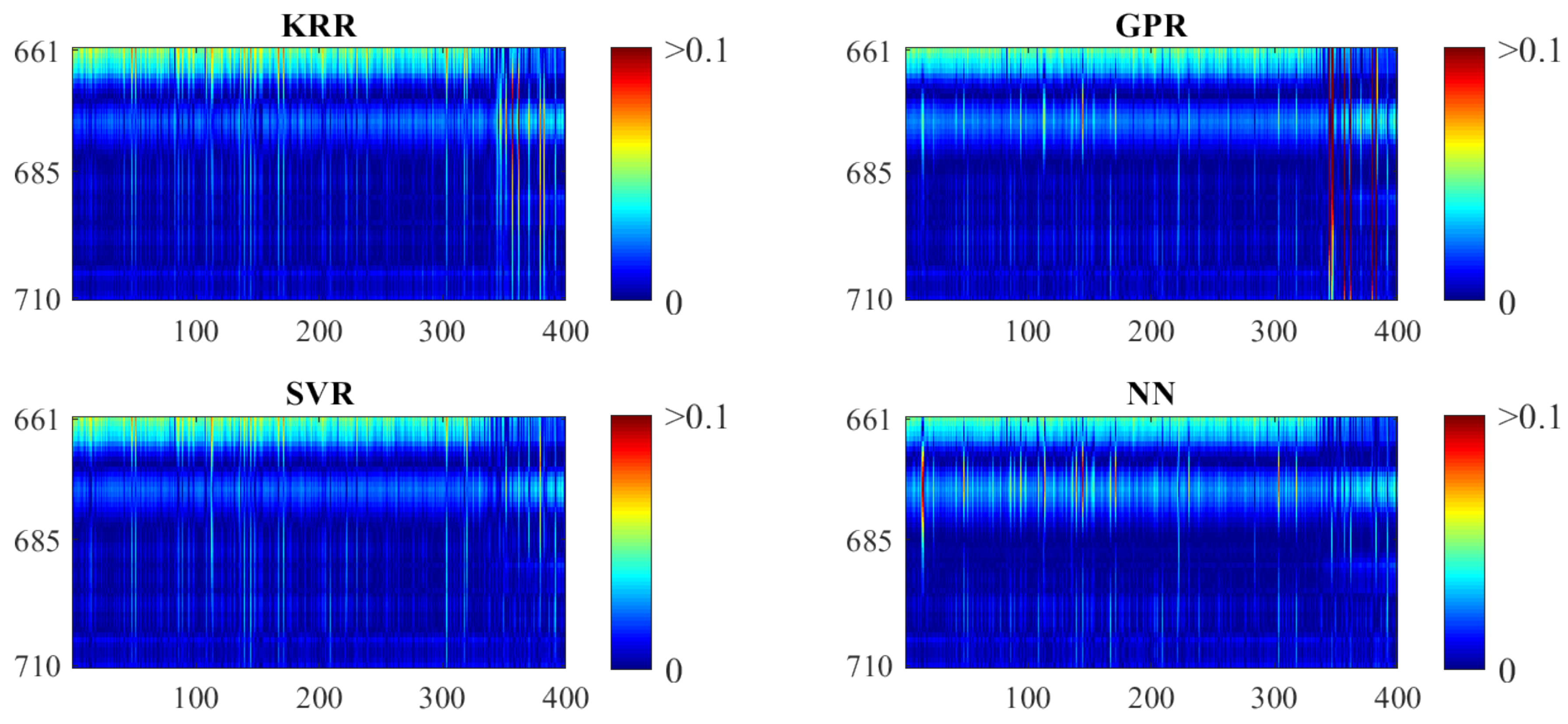
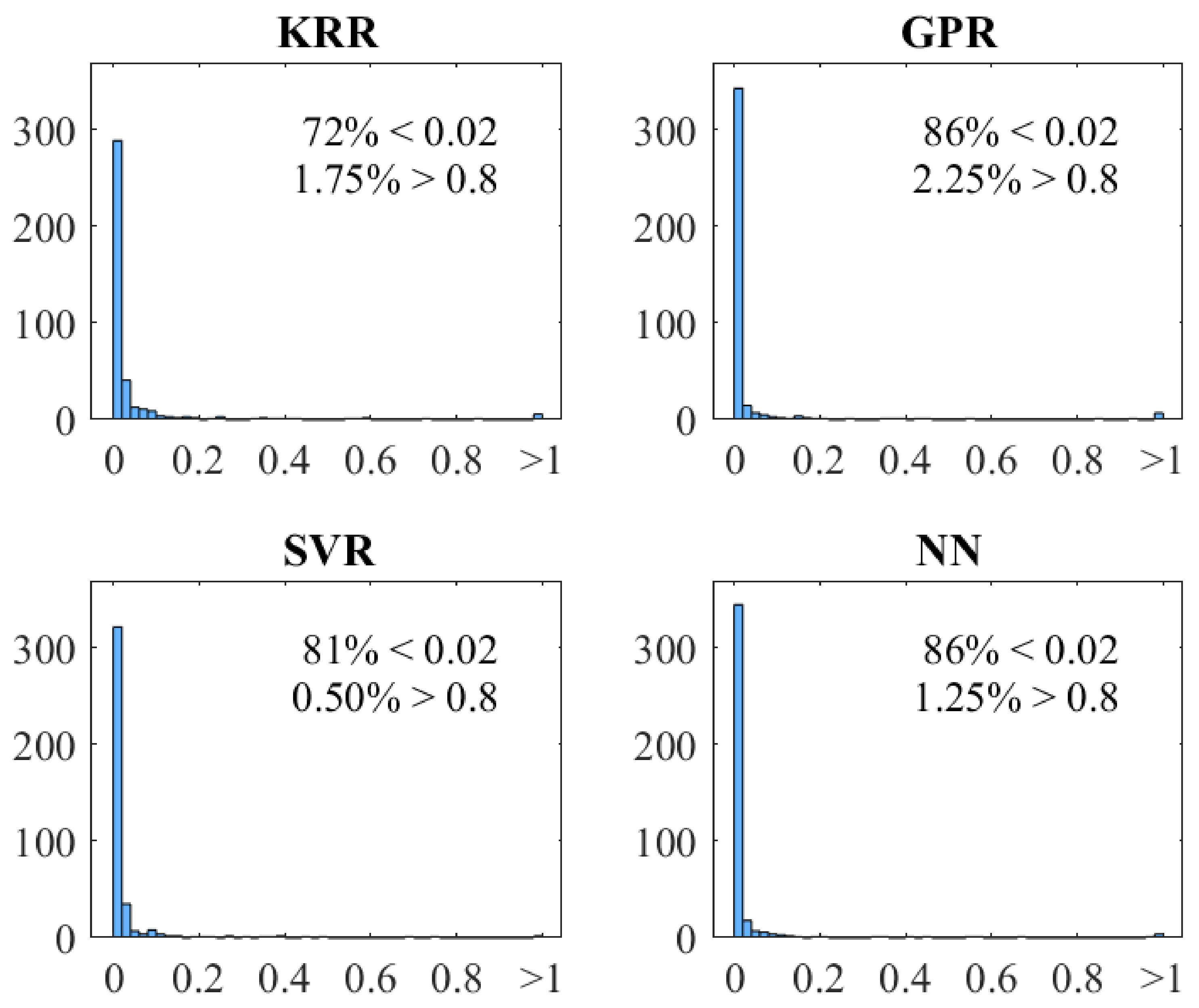
5.2. Validation of the Normalized Remote-Sensing Reflectance without SICF Contribution ($Rrs{n}_{-SICF}(\lambda )$) Estimation

The “observed data” from the VDB was used as input to test the performance of different MLRA methods. Once the three anchor points into the “inside range” were estimated by each MLRA method, the cubic spline fitting was performed to estimate the $Rrs{n}_{-SICF}\left(\lambda \right)$. Next, the estimated $Rrs{n}_{-SICF}\left(\lambda \right)$ was compared with the “reference data” from VDB to evaluate each MLRA method.

The relative error ((reference value-estimated value)/reference value) for the estimated $Rrs{n}_{-SICF}\left(\lambda \right)$ in the “inside range” (661–710 nm) was calculated for each band in the “inside range” for all the 400 spectra from the VDB (Figure 7). All four MLRA methods showed similar performance, resulting in maximum errors near to 0.1, with RMSE values lower than 0.1 and RRMSE values close to 0.02 (

Table 3. Summary of statistical results and training/testing time of validation of each MLRA trained to estimate $Rrs{n}_{-SICF}\left(\lambda \right)$.

MLRA	R2	RMSE	RRMSE	Training Time (s)	Testing Time (s)
KRR	0.99	0.10	0.02	19,241	0.004
GPR	0.97	0.20	0.05	61,732	0.002
SVR	0.99	0.09	0.02	519,335	0.014
NN	0.99	0.10	0.02	73,891	0.003

), except GPR with errors up to 0.8 in some samples and with an RRMSE value of 0.05. However, SVR showed a more accurate retrieval, with 0% of samples with errors >0.8 (Figure 8).

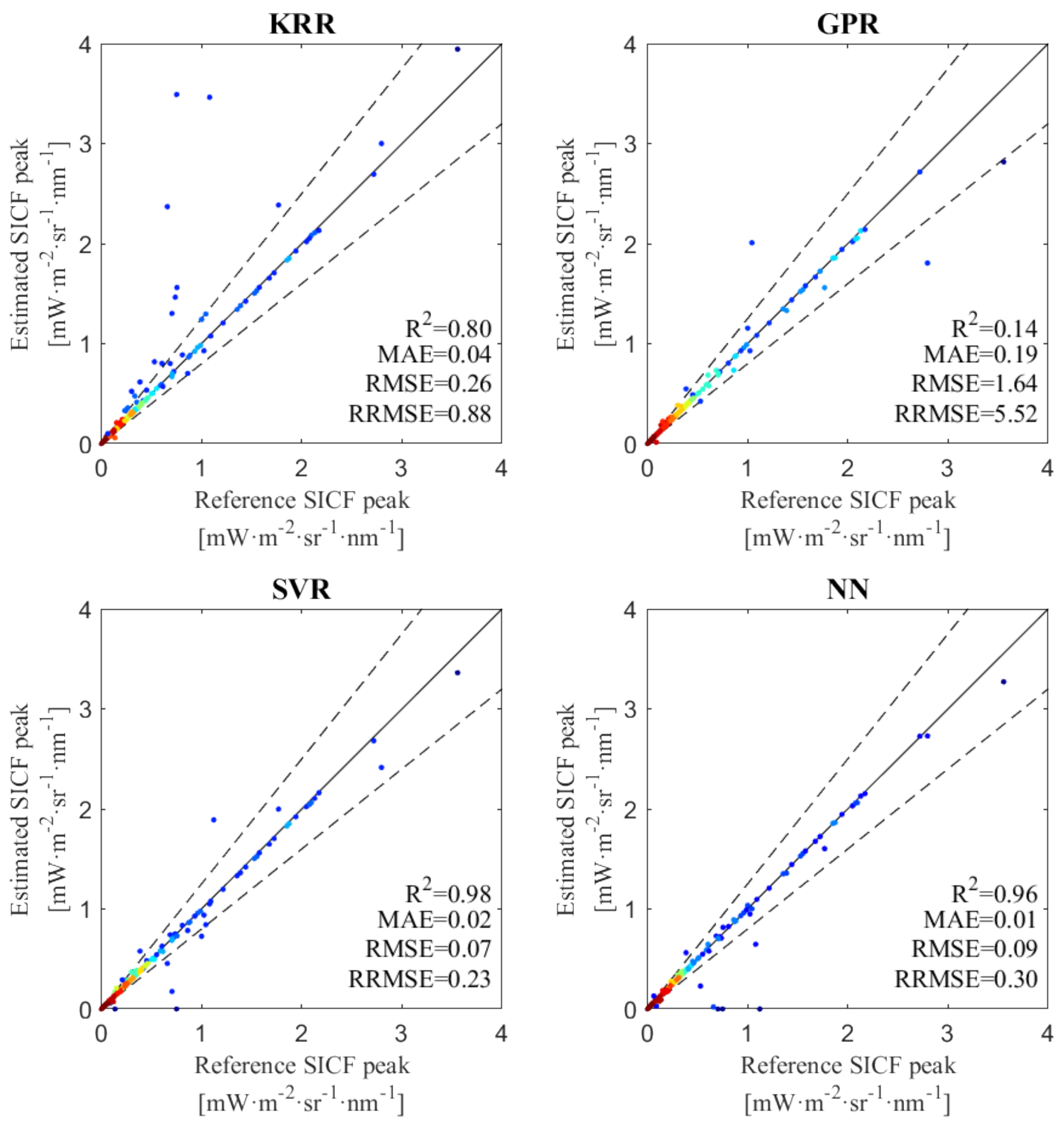
5.3. Validation of Sun Induced Chlorophyll Fluorescence (SICF) Estimation

Once $Rr{s}_{-SICF}\left(\lambda \right)$ was estimated, SICF was calculated according to Equations (12)–(14). The relative error between the reference and retrieved SICF peak (SICF at 685 nm) from the VDB was calculated. A relative error of less than 2% was obtained for the four MLRA methods in more than 70% of the samples. SVR showed the least number of samples with errors >0.8 (0.5%) (Figure 9).

The scatterplots in Figure 10 show that all MLRA methods performed a good estimation of SICF peak (at 685 nm), except the GPR, with an R² = 0.14 and an RRMSE greater than 5. The best estimation was performed by using SVR, obtaining an R² = 0.98 and an RRMSE lower than 0.25.

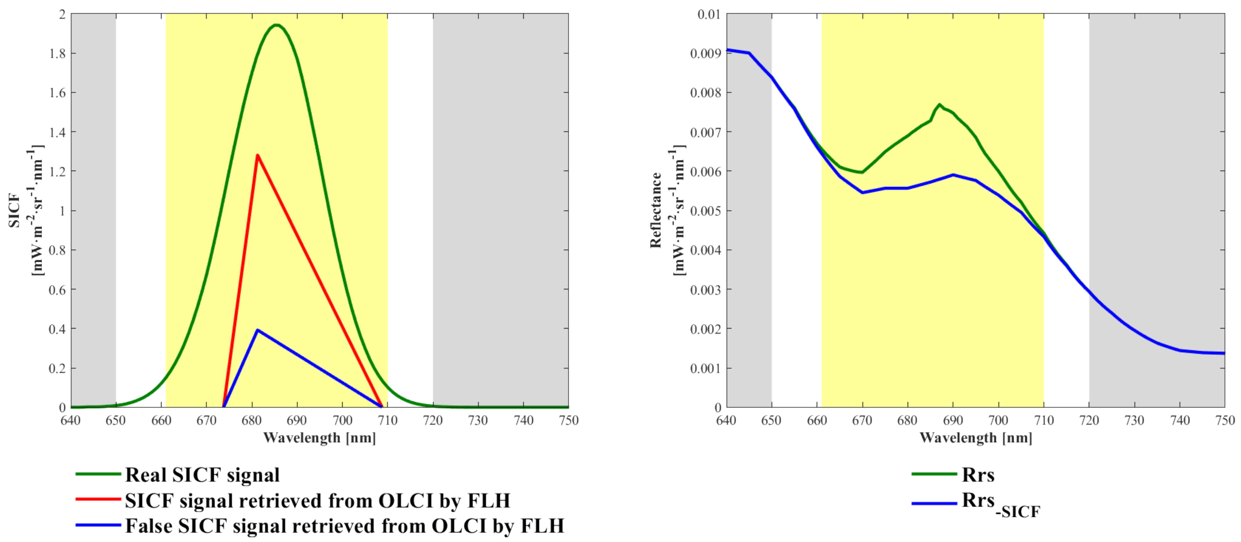
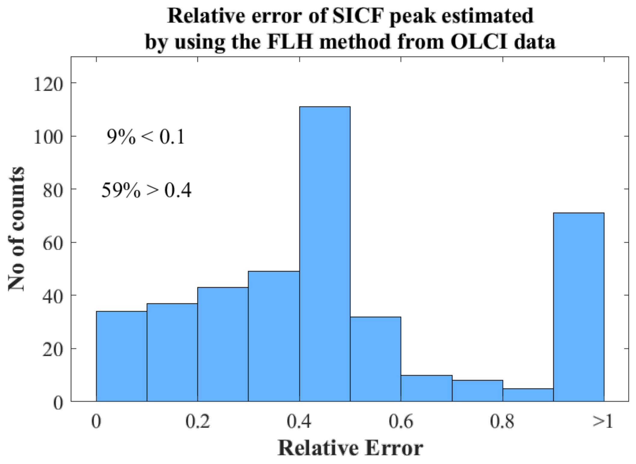
5.4. Comparison of the Proposed Sun Induced Chlorophyll Fluorescence (SICF) Retrieval Method with the Fluorescence Line Height (FLH) Method

To compare SICF obtained by using the algorithm here proposed, from a high spectral resolution reflectance, with the SICF that would be obtained from the ocean and land color instrument (OLCI) by using the FLH method, the spectra of the VDB were convolved to the instrument spectral response function (ISRF) of OLCI, followed by the application of the FLH method and comparison with our algorithm. To illustrate the effect of the reflectance shoulder (or peak) beneath the SICF emission peak, the FLH for OLCI was not only calculated from $Rrs\left(\lambda \right)$, as in its normal operation (red line in Figure 11), but also from the simulated $Rr{s}_{-SICF}\left(\lambda \right)$, without fluorescence (blue line in Figure 11). Two issues are evident from the spectra shown in Figure 11: (1) the FLH from OLCI underestimated the actual SICF emission, and (2) part of the retrieved OLCI FLH did not correspond to fluorescence, but to “residual” reflectance above the baseline. Both effects can lead to misinterpretations of the meaning of the FLH.

To compare our results on SICF estimation with the original FLH method, the VDB was convolved to the OLCI ISRF, to which the FLH method was applied.

Similar to our previous analyses, the relative error of the SICF peak between this retrieval and the “reference” integrated SICF was calculated (Figure 12), showing that the FLH method was only able to obtain 9% of cases with a less than 10% relative error, while the majority of the cases showed a relative error higher than 40%.

The SICF peak is a distinct feature in water-leaving remote sensing reflectance, which adds to the “background” reflectance in the 660–750 nm region. In clear ocean waters, that background is roughly linear with a negative slope towards the infrared, and this is the basis of the baseline approach commonly used for fluorescence retrieval. However, in productive coastal waters, the combined effects of particle scattering and phytoplankton and water absorption creates a reflectance shoulder or even a peak in the 670–720 nm region, invalidating the baseline approach based on two wavelengths outside the SICF emission peak.

This effect was thoroughly described in [22,23] and affects FLH use as a proxy for the actual SICF emission. In the most extreme cases (very high [Chla]) the peak is entirely dependent on backscattering, due to the strong Chla reabsorption of the fluorescence emission. The only way to estimate the actual SICF curve is to decouple the emission from the background reflectance. Since both signals are combined in actual measurements, it is necessary to estimate somehow the background. The unavailability of SICF in-situ data, limits the validation of the algorithm. Measurements of [Chla] or in-situ fluorescence (measured using artificial light sources) as proxies of SICF could be used to validate it; however, it should be taken into account that the use of this data is not free of biases and errors. The relationship of SICF and [Chla] is not linear, and for the high [Chla] found in productive waters, the contribution of particulate scattering to the fluorescence peak invalids the use of a baseline approximation in the fluorescence peak for SICF retrieval.

6. Conclusions

The development and testing of a new method for the retrieval of SICF of coastal and ocean waters is presented in this work. The algorithm first performs a normalization of the observed apparent ($Rrs$) reflectance at 780 nm (following the similarity index approximation), followed by the fitting of the normalized reflectance without fluorescence contribution. This proposed fitting is based on the estimation of three reflectance anchor points within the SICF emission range, by using MLRAs methods and adjusting the normalized true reflectance spectra with a cubic spline fitting.

A training database composed of 7200 $Rrs{n}_{-SICF}\left(\lambda \right)$ spectra designed to typify the high spectral variability in coastal and ocean waters affected by a wide range of Chla contents and CDOM was used to test the algorithm. The validation database was simulated for these typical ranges too, while using different forward formulations and adding non-algal particles (NAP) to reduce consistency with the calibration database. The approach of estimating the shape of the true reflectance or $Rr{s}_{-SICF}\left(\lambda \right)$ from the $Rrs{n}_{-SICF}\left(\lambda \right)$ shape, obtained from the anchor point fitting inside the SICF emission range of $Rrsn\left(\lambda \right)$, allows the SICF signal to be discriminated from the “shoulder” produced by the absorption/scattering of the OAC in water. All four tested MLRA methods showed similar results for the retrieval of $Rrs{n}_{-SICF}\left(\lambda \right)$, but the GPR method showed relative errors > 0.8 in a small part of the samples, while lower error values were obtained by using SVR.

The final SICF validation using a validation database with simulated SICF resulted in relative errors close to 2% in the estimation of $Rrs{n}_{-SICF}\left(\lambda \right)$ and relative errors lower than 2% in more than 70% of the samples in the SICF peak retrieval. When applied to simulated OLCI bands, the proposed SICF retrieval method significantly improved the regular method to retrieve detectable SICF based on the FLH algorithm, as the latter resulted in relative errors higher than 40% in 59% of the samples.

The newly proposed method can be applied for future satellite missions such as FLEX [27] and CHIME [28], which will provide a more detailed spectral shape of water-leaving radiance. A higher accuracy in SICF retrievals from these sensors will provide better insights into the functioning and productivity of ocean and coastal phytoplankton.

References

1. Behrenfeld, M.J.; Westberry, T.K.; Boss, E.S.; O’Malley, R.T.; Siegel, D.A.; Wiggert, J.D.; Franz, B.A.; McClain, C.R.; Feldman, G.C.; Doney, S.C.; et al. Satellite-Detected Fluorescence Reveals Global Physiology of Ocean Phytoplankton. Biogeosciences 2009, 6, 779–794. [Google Scholar] [CrossRef] [Green Version]
2. Joseph, A. Chapter 10—Magic With Colors Sea Surface Changes. In Investigating Seafloors and Oceans; Joseph, A., Ed.; Elsevier: Amsterdam, The Netherlands, 2017; pp. 555–574. ISBN 978-0-12-809357-3. [Google Scholar]
3. Ling, Z.; Sun, D.; Wang, S.; Qiu, Z.; Huan, Y.; Mao, Z.; He, Y. Retrievals of Phytoplankton Community Structures from in Situ Fluorescence Measurements by HS-6P. Opt. Express 2018, 26, 30556–30575. [Google Scholar] [CrossRef]
4. Huot, Y.; Babin, M. Overview of Fluorescence Protocols: Theory, Basic Concepts, and Practice. In Chlorophyll a Fluorescence in Aquatic Sciences: Methods and Applications; Suggett, J.D., Prášil, O., Borowitzka, A.M., Eds.; Springer: Dordrecht, The Netherlands, 2010; pp. 31–74. ISBN 978-90-481-9268-7. [Google Scholar]
5. Gower, J.F.R.; Doerffer, R.; Borstad, G.A. Interpretation of the 685 Nm Peak in Water-Leaving Radiance Spectra in Terms of Fluorescence, Absorption and Scattering, and Its Observation by MERIS. Int. J. Remote Sens. 1999, 20, 1771–1786. [Google Scholar] [CrossRef]
6. Maritorena, S.; Morel, A.; Gentili, B. Determination of the Fluorescence Quantum Yield by Oceanic Phytoplankton in Their Natural Habitat. Appl. Opt. 2000, 39, 6725–6737. [Google Scholar] [CrossRef] [PubMed]
7. Laney, S.R. Chlorophyll a Fluorescence in Aquatic Sciences: Methods and Applications; Suggett, J.D., Prášil, O., Borowitzka, A.M., Eds.; Springer: Dordrecht, The Netherlands, 2010; pp. 19–30. ISBN 978-90-481-9268-7. [Google Scholar]
8. Westberry, T.K.; Behrenfeld, M.J.; Milligan, A.J.; Doney, S.C. Retrospective Satellite Ocean Color Analysis of Purposeful and Natural Ocean Iron Fertilization. Deep Sea Res. Part Oceanogr. Res. Pap. 2013, 73, 1–16. [Google Scholar] [CrossRef]
9. Escoffier, N.; Bernard, C.; Hamlaoui, S.; Groleau, A.; Catherine, A. Quantifying Phytoplankton Communities Using Spectral Fluorescence: The Effects of Species Composition and Physiological State. J. Plankton Res. 2014. [Google Scholar] [CrossRef]
10. Huot, Y.; Brown, C.A.; Cullen, J.J. New Algorithms for MODIS Sun-Induced Chlorophyll Fluorescence and a Comparison with Present Data Products. Limnol. Oceanogr. Methods 2005, 3, 108–130. [Google Scholar] [CrossRef] [Green Version]
11. Huot, Y.; Brown, C.A.; Cullen, J.J. Retrieval of Phytoplankton Biomass from Simultaneous Inversion of Reflectance, the Diffuse Attenuation Coefficient, and Sun-Induced Fluorescence in Coastal Waters. J. Geophys. Res. Oceans 2007, 112, C06013. [Google Scholar] [CrossRef] [Green Version]
12. Huot, Y.; Babin, M.; Bruyant, F.; Grob, C.; Twardowski, M.S.; Claustre, H. Relationship between Photosynthetic Parameters and Different Proxies of Phytoplankton Biomass in the Subtropical Ocean. Biogeosciences 2007, 4, 853–868. [Google Scholar] [CrossRef] [Green Version]
13. Abbott, M.R.; Letelier, R.M. Algorithm Theoretical Basis Document Chlorophyll Fluorescence (MODIS Product Number 20); NASA: Corvallis, OR, USA, 1999. [Google Scholar]
14. Kolber, Z.; Falkowski, P.G. Use of Active Fluorescence to Estimate Phytoplankton Photosynthesis in Situ. Limnol. Oceanogr. 1993, 38, 1646–1665. [Google Scholar] [CrossRef]
15. Lin, H.; Kuzminov, F.I.; Park, J.; Lee, S.; Falkowski, P.G.; Gorbunov, M.Y. The Fate of Photons Absorbed by Phytoplankton in the Global Ocean. Science 2016, 351, 264–267. [Google Scholar] [CrossRef] [PubMed]
16. Neville, R.A.; Gower, J.F.R. Passive Remote Sensing of Phytoplankton via Chlorophyll a Fluorescence. J. Geophys. Res. 1977, 82, 3487–3493. [Google Scholar] [CrossRef]
17. Babin, M.; Morel, A.; Gentili, B. Remote Sensing of Sea Surface Sun-Induced Chlorophyll Fluorescence: Consequences of Natural Variations in the Optical Characteristics of Phytoplankton and the Quantum Yield of Chlorophyll a Fluorescence. Int. J. Remote Sens. 1996, 17, 2417–2448. [Google Scholar] [CrossRef]
18. Gower, J.F.R.; Borstad, G.A. On the Potential of MODIS and MERIS for Imaging Chlorophyll Fluorescence from Space. Int. J. Remote Sens. 2004, 25, 1459–1464. [Google Scholar] [CrossRef]
19. Letelier, R.M.; Abbott, M.R. An Analysis of Chlorophyll Fluorescence Algorithms for the Moderate Resolution Imaging Spectrometer (MODIS). Remote Sens. Environ. 1996, 58, 215–223. [Google Scholar] [CrossRef]
20. Zhao, D.; Xing, X.; Liu, Y.; Yang, J.; Wang, L. The Relation of Chlorophyll-a Concentration with the Reflectance Peak near 700 Nm in Algae-Dominated Waters and Sensitivity of Fluorescence Algorithms for Detecting Algal Bloom. Int. J. Remote Sens. 2010, 31, 39–48. [Google Scholar] [CrossRef]
21. Gower, J.F.R.; Brown, L.; Borstad, G.A. Observation of Chlorophyll Fluorescence in West Coast Waters of Canada Using the MODIS Satellite Sensor. Can. J. Remote Sens. 2004, 30, 17–25. [Google Scholar] [CrossRef]
22. Gilerson, A.; Zhou, J.; Oo, M.; Chowdhary, J.; Gross, B.M.; Moshary, F.; Ahmed, S. Retrieval of Chlorophyll Fluorescence from Reflectance Spectra through Polarization Discrimination: Modeling and Experiments. Appl. Opt. 2006, 45, 5568–5581. [Google Scholar] [CrossRef]
23. Gilerson, A.; Zhou, J.; Hlaing, S.; Ioannou, I.; Schalles, J.; Gross, B.; Moshary, F.; Ahmed, S. Fluorescence Component in the Reflectance Spectra from Coastal Waters. Dependence on Water Composition. Opt. Express 2007, 15, 15702–15721. [Google Scholar] [CrossRef]
24. Gitelson, A.A.; Schalles, J.F.; Hladik, C.M. Remote Chlorophyll-a Retrieval in Turbid, Productive Estuaries: Chesapeake Bay Case Study. Remote Sens. Environ. 2007, 109, 464–472. [Google Scholar] [CrossRef]
25. Zhou, J.; Gilerson, A.; Ioannou, I.; Hlaing, S.; Schalles, J.; Gross, B.; Moshary, F.; Ahmed, S. Retrieving Quantum Yield of Sun-Induced Chlorophyll Fluorescence near Surface from Hyperspectral in-Situ Measurement in Productive Water. Opt. Express 2008, 16, 17468–17483. [Google Scholar] [CrossRef] [PubMed]
26. Gilerson, A.A.; Huot, Y. Chapter 7—Bio-optical Modeling of Sun-Induced Chlorophyll-a Fluorescence. In Bio-Optical Modeling and Remote Sensing of Inland Waters; Mishra, D.R., Ogashawara, I., Gitelson, A.A., Eds.; Elsevier: Amsterdam, The Netherlands, 2017; pp. 189–231. ISBN 978-0-12-804644-9. [Google Scholar]
27. Drusch, M.; Moreno, J.; Bello, U.D.; Franco, R.; Goulas, Y.; Huth, A.; Kraft, S.; Middleton, E.M.; Miglietta, F.; Mohammed, G.; et al. The FLuorescence EXplorer Mission Concept-ESA’s Earth Explorer 8. IEEE Trans. Geosci. Remote Sens. 2017, 55, 1273–1284. [Google Scholar] [CrossRef]
28. Nieke, J.; Rast, M. Towards the Copernicus Hyperspectral Imaging Mission For The Environment (CHIME). In Proceedings of the IGARSS 2018—2018 IEEE International Geoscience and Remote Sensing Symposium, Valencia, Spain, 22–27 July 2018; pp. 157–159. [Google Scholar]
29. Ruddick, K.G.; De Cauwer, V.; Park, Y.-J.; Moore, G. Seaborne Measurements of near Infrared Water-Leaving Reflectance: The Similarity Spectrum for Turbid Waters. Limnol. Oceanogr. 2006, 51, 1167–1179. [Google Scholar] [CrossRef] [Green Version]
30. Pope, R.M.; Fry, E.S. Absorption Spectrum (380-700 Nm) of Pure Water. II. Integrating Cavity Measurements. Appl. Opt. 1997, 36, 8710–8723. [Google Scholar] [CrossRef] [PubMed]
31. Bricaud, A.; Morel, A.; Prieur, L. Absorption by Dissolved Organic Matter of the Sea (Yellow Substance) in the UV and Visible Domains1. Limnol. Oceanogr. 1981, 26, 43–53. [Google Scholar] [CrossRef]
32. Mobley, C.D. Light and Water: Radiative Transfer in Natural Waters; Academic Press: Cambridge, MA, USA, 1994. [Google Scholar]
33. Morel, A. Optical Modeling of the Upper Ocean in Relation to Its Biogenous Matter Content (Case I Waters). J. Geophys. Res. Oceans 1988, 93, 10749–10768. [Google Scholar] [CrossRef] [Green Version]
34. Prieur, L.; Sathyendranath, S. An Optical Classification of Coastal and Oceanic Waters Based on the Specific Spectral Absorption Curves of Phytoplankton Pigments, Dissolved Organic Matter, and Other Particulate Materials1. Limnol. Oceanogr. 1981, 26, 671–689. [Google Scholar] [CrossRef]
35. Mobley, C.D. HydroLight 4.0 Technical Documentation; Sequoia Scientific, Inc.: Mercer Island, WA, USA, 2008. [Google Scholar]
36. Boss, E.; Twardowski, M.S.; Herring, S. Shape of the Particulate Beam Attenuation Spectrum and Its Inversion to Obtainthe Shape of the Particulate Size Distribution. Appl. Opt. 2001, 40, 4885–4893. [Google Scholar] [CrossRef]
37. Loisel, H.; Morel, A. Light Scattering and Chlorophyll Concentration in Case 1 Waters: A Reexamination. Limnol. Oceanogr. 1998, 43, 847–858. [Google Scholar] [CrossRef] [Green Version]
38. Doxaran, D.; Ruddick, K.; McKee, D.; Gentili, B.; Tailliez, D.; Chami, M.; Babin, M. Spectral Variations of Light Scattering by Marine Particles in Coastal Waters, from the Visible to the near Infrared. Limnol. Oceanogr. 2009, 54, 1257–1271. [Google Scholar] [CrossRef] [Green Version]
39. Mobley, C.D.; Sundman, L.K.; Boss, E. Phase Function Effects on Oceanic Light Fields. Appl. Opt. 2002, 41, 1035–1050. [Google Scholar] [CrossRef] [PubMed] [Green Version]
40. McKee, D.; Cunningham, A.; Wright, D.; Hay, L. Potential Impacts of Nonalgal Materials on Water-Leaving Sun Induced Chlorophyll Fluorescence Signals in Coastal Waters. Appl. Opt. 2007, 46, 7720–7729. [Google Scholar] [CrossRef] [PubMed]
41. Kirk, J.T. Light and Photosynthesis in Aquatic Ecosystems, 3rd ed.; Cambridge University Press: Cambridge, UK, 2011. [Google Scholar]
42. Doxaran, D.; Babin, M.; Leymarie, E. Near-Infrared Light Scattering by Particles in Coastal Waters. Opt. Express 2007, 15, 12834–12849. [Google Scholar] [CrossRef] [PubMed]
43. Sipelgas, L.; Raudsepp, U. Comparison of Hyperspectral Measurements of the Attenuation and Scattering Coefficients Spectra with Modeling Results in the North-Eastern Baltic Sea. Estuar. Coast. Shelf Sci. 2015, 165, 1–9. [Google Scholar] [CrossRef] [Green Version]
44. Ahn, Y. Proprietes Optiques Des Particules Biologiques et Minerales. Ph.D. Thesis, Universite Pierre et Marie Curie, Paris, France, 1999. [Google Scholar]
45. Bukata, R.P.; Jerome, J.H.; Kondratyev, A.S.; Pozdnyakov, D.V. Optical Properties and Remote Sensing of Inland and Coastal Waters; CRC Press: Boca Raton, FL, USA, 2018. [Google Scholar]
46. Gilerson, A.; Zhou, J.; Hlaing, S.; Ioannou, I.; Gross, B.; Moshary, F.; Ahmed, S. Fluorescence Component in the Reflectance Spectra from Coastal Waters. II. Performance of Retrieval Algorithms. Opt. Express 2008, 16, 2446–2460. [Google Scholar] [CrossRef]
47. Fournier, G.R.; Forand, J.L. Analytic Phase Function for Ocean Water. In Proceedings of the SPIE—The International Society for Optical Engineering: Ocean Optics XII, Bergen, Norway, 26 October 1994; Volume 2258, pp. 194–201. [Google Scholar]
48. Morel, A.; Antoine, D.; Gentili, B. Bidirectional Reflectance of Oceanic Waters: Accounting for Raman Emission and Varying Particle Scattering Phase Function. Appl. Opt. 2002, 41, 6289–6306. [Google Scholar] [CrossRef]
49. Rivera-Caicedo, J.P.; Verrelst, J.; Muñoz-Marí, J.; Moreno, J.; Camps-Valls, G. Toward a Semiautomatic Machine Learning Retrieval of Biophysical Parameters. IEEE J. Sel. Top. Appl. Earth Obs. Remote Sens. 2014, 7, 1249–1259. [Google Scholar] [CrossRef]
50. Verrelst, J.; Muñoz, J.; Alonso, L.; Delegido, J.; Rivera, J.P.; Camps-Valls, G.; Moreno, J. Machine Learning Regression Algorithms for Biophysical Parameter Retrieval: Opportunities for Sentinel-2 and -3. Remote Sens. Environ. 2012, 118, 127–139. [Google Scholar] [CrossRef]
51. Bacour, C.; Baret, F.; Béal, D.; Weiss, M.; Pavageau, K. Neural Network Estimation of LAI, FAPAR, FCover and LAI×Cab, from Top of Canopy MERIS Reflectance Data: Principles and Validation. Remote Sens. Environ. 2006, 105, 313–325. [Google Scholar] [CrossRef]
52. Borchani, H.; Varando, G.; Bielza, C.; Larrañaga, P. A Survey on Multi-Output Regression. Wiley Interdiscip. Rev. Data Min. Knowl. Discov. 2015, 5, 216–233. [Google Scholar] [CrossRef] [Green Version]
53. Shawe-Taylor, J.; Cristianini, N. Kernel Methods for Pattern Analysis; Cambridge University Press: Cambridge, UK, 2004. [Google Scholar]
54. Camps-Valls, G.; Munoz-Mari, J.; Gomez-Chova, L.; Guanter, L.; Calbet, X. Nonlinear Statistical Retrieval of Atmospheric Profiles From MetOp-IASI and MTG-IRS Infrared Sounding Data. IEEE Trans. Geosci. Remote Sens. 2012, 50, 1759–1769. [Google Scholar] [CrossRef]
55. Rasmussen, C.E.; Williams, C.K. Gaussian Processes for Machine Learning; The MIT Press: Cambridge, MA, USA, 2006; ISBN 0-262-18253-X. [Google Scholar]
56. Camps-Valls, G.; Bruzzone, L.; Rojo-Alvarez, J.L.; Melgani, F. Robust Support Vector Regression for Biophysical Variable Estimation from Remotely Sensed Images. IEEE Geosci. Remote Sens. Lett. 2006, 3, 339–343. [Google Scholar] [CrossRef]
57. Bishop, C.M. Neural Networks for Pattern Recognition; Oxford University Press: Oxford, UK, 1995. [Google Scholar]
Figure 1. (Left): Illustration of the fluorescence line height (FLH) algorithm for an example showing the water-leaving radiance with and without sun induced chlorophyll fluorescence (SICF) contribution. The λ 1 , λ 2 , and λ 3 bands correspond to the band centers 667, 668, and 746 nm for MODIS and 665, 684, and 709 or 753 nm for OLCI. The difference between the apparent and true water-leaving radiance corresponds to the SICF signal. (Right): Equivalent remote sensing reflectance.
Remotesensing 13 00329 g001
Figure 2. The 7200 remote sensing reflectance without SICF contribution, R r s n S I C F (left), and remote sensing reflectance without SICF contribution normalized at 780 nm, R r s n S I C F (right), simulated spectra using the settings described in Table 1. It is noted that the spectral variability is very low in the NIR spectral range (>720 nm).
Remotesensing 13 00329 g002
Figure 3. Obtained SICF from the simulated VDB.
Remotesensing 13 00329 g003
Figure 4. Graphic explanation of the R r s n S I C F λ retrieval concept. The green spectrum corresponds to the “observed data” (from a radiometer or remote sensor) R r s n λ . The black diamonds indicate the three anchor points estimated by using MLRA methods. The blue spectrum is the R r s n S I C F λ “reference spectra” from the simulated training database and the orange spectrum is the R r s n S I C F λ “estimated spectra” calculating the cubic spline fitting using the bands in the “outside ranges” (green diamonds) and the three anchor points. It is observed that R r s n S I C F λ has a “shoulder” produced by the absorption/scattering effects from OACs.
Remotesensing 13 00329 g004
Figure 5. Scheme summarizing the methodology followed in the development of the SICF retrieval algorithm.
Remotesensing 13 00329 g005
Figure 6. (a) Three examples from the database of 7200 spectra showing the comparison of normalized remote-sensing reflectance without SICF contribution ( R r s n S I C F ( λ ) ) spectra (blue) with its corresponding spline adjustment (black). (b) Normalized remote-sensing reflectance without SICF contribution ( R r s n S I C F ( λ ) ) vs. adjusted normalized remote-sensing reflectance without SICF contribution in the spectral range between 640 and 750 nm for all the wavelengths in this range.
Remotesensing 13 00329 g006
Figure 7. Relative error between the “reference data” from VDB and the retrieved R r s n S I C F λ in the spectral range between 661 and 710 nm for each MLRA trained. The X-axis is the number of validated spectra (1 to 400) and the Y-axis are the wavelengths of the estimated bands. The scale color represents the relative error values, the blue being the lower errors, and the red being the higher errors.
Remotesensing 13 00329 g007
Figure 8. Histograms of the relative errors for all bands in the spectral range between 661 and 710 nm between the spectra of the “reference data” from VDB and the retrieved R r s n S I C F λ for each MLRA trained. The X-axis is the relative error and the Y-axis are the number of counts.
Remotesensing 13 00329 g008
Figure 9. Histograms of the relative errors between the “reference data” from VDB and the estimated SICF peak (at 685 nm), with each MLRA retrieval method used to estimate the intermediate ρ w n . The X-axis is the relative error and the Y-axis is the number of counts.
Remotesensing 13 00329 g009
Figure 10. Scatterplot of reference SICF peak vs. estimated SICF peak (at 685 nm) for each MLRA retrieval method used to estimate the intermediate R r s n S I C F λ . The color dots correspond to the density of samples, the red zones being higher and the blue zones lower. The dashed line corresponds to the limit of 20% of error.
Remotesensing 13 00329 g010
Figure 11. Left: SICF retrieved from the simulated validation data, using Equation (14) (green line), SICF retrieved from simulated validation data convolved to the OLCI ISRF (red line), and SICF retrieved from simulated validation data “without SICF” convolved to the OLCI ISRF (blue line). Right: R r s spectrum of SICF in left figure (green line). R r s S I C F spectrum of false SICF in left figure (blue line).
Remotesensing 13 00329 g011
Figure 12. Histogram of the relative errors between the “reference” SICF peak and the estimated SICF peak by using FLH method over convolved data to OLCI ISRF. The X-axis is the relative error, and the Y-axis is the number of counts.
Remotesensing 13 00329 g012