
The Spatio-Temporal Variability of Frost Blisters in a Perennial Frozen Lake along the Antarctic Coast as Indicator of the Groundwater Supply


Abstract
:1. Introduction
2. Materials and Methods
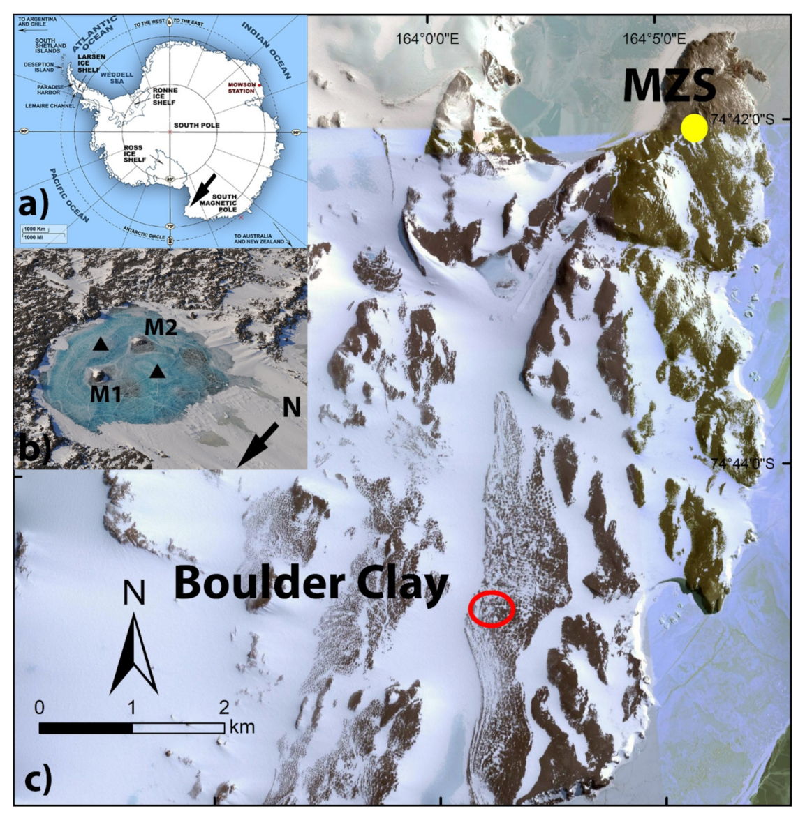
2.1. Study Area and Climate Analyses
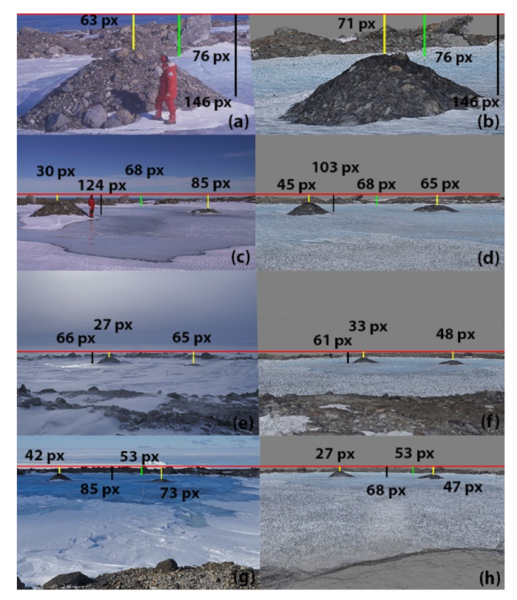
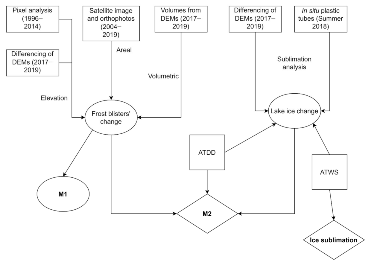
2.2. Photogrammetric Analysis
2.3. DEM Analysis and Sublimation Rates
3. Results
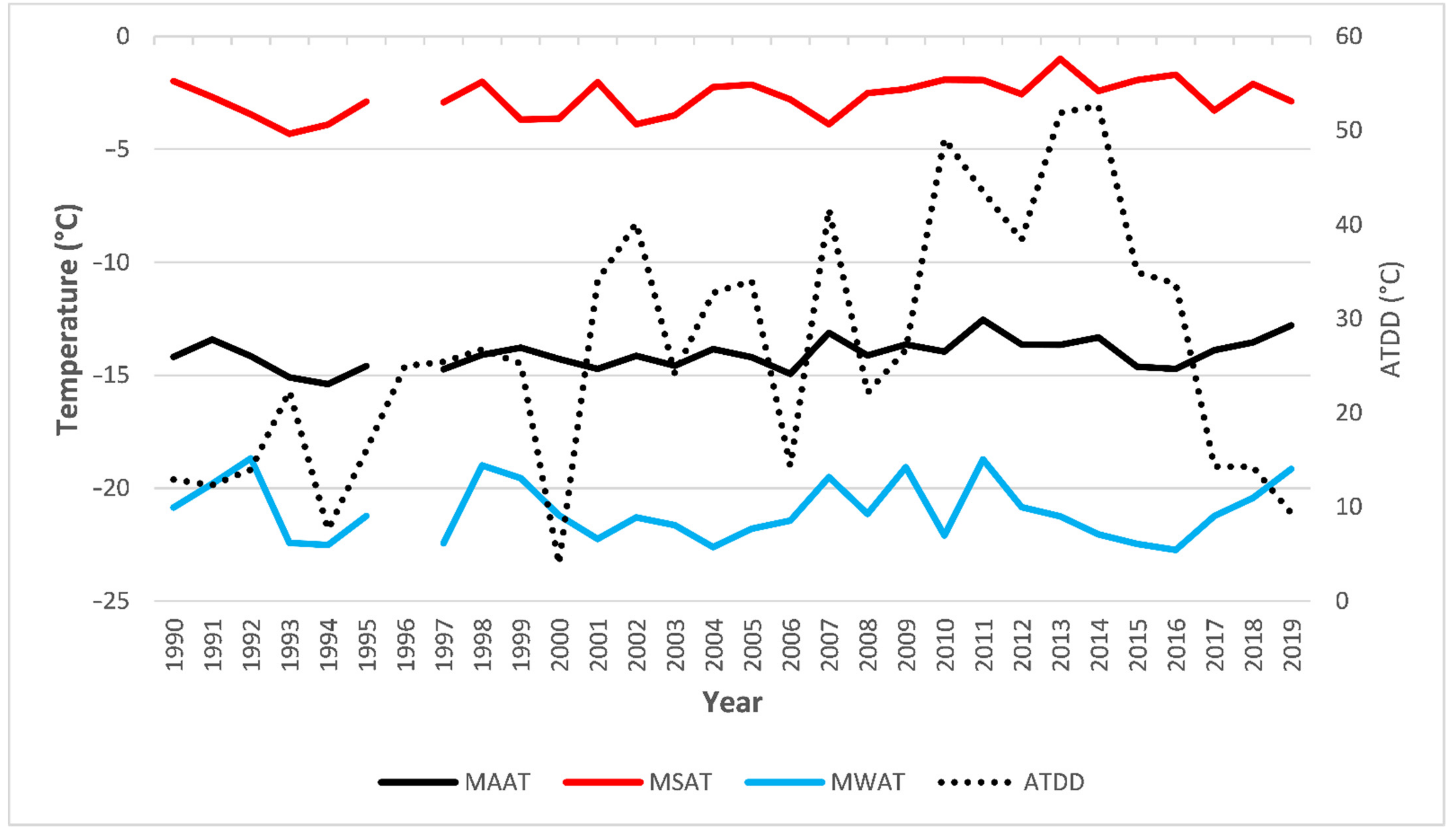
3.1. Climate
3.2. Frost Blisters
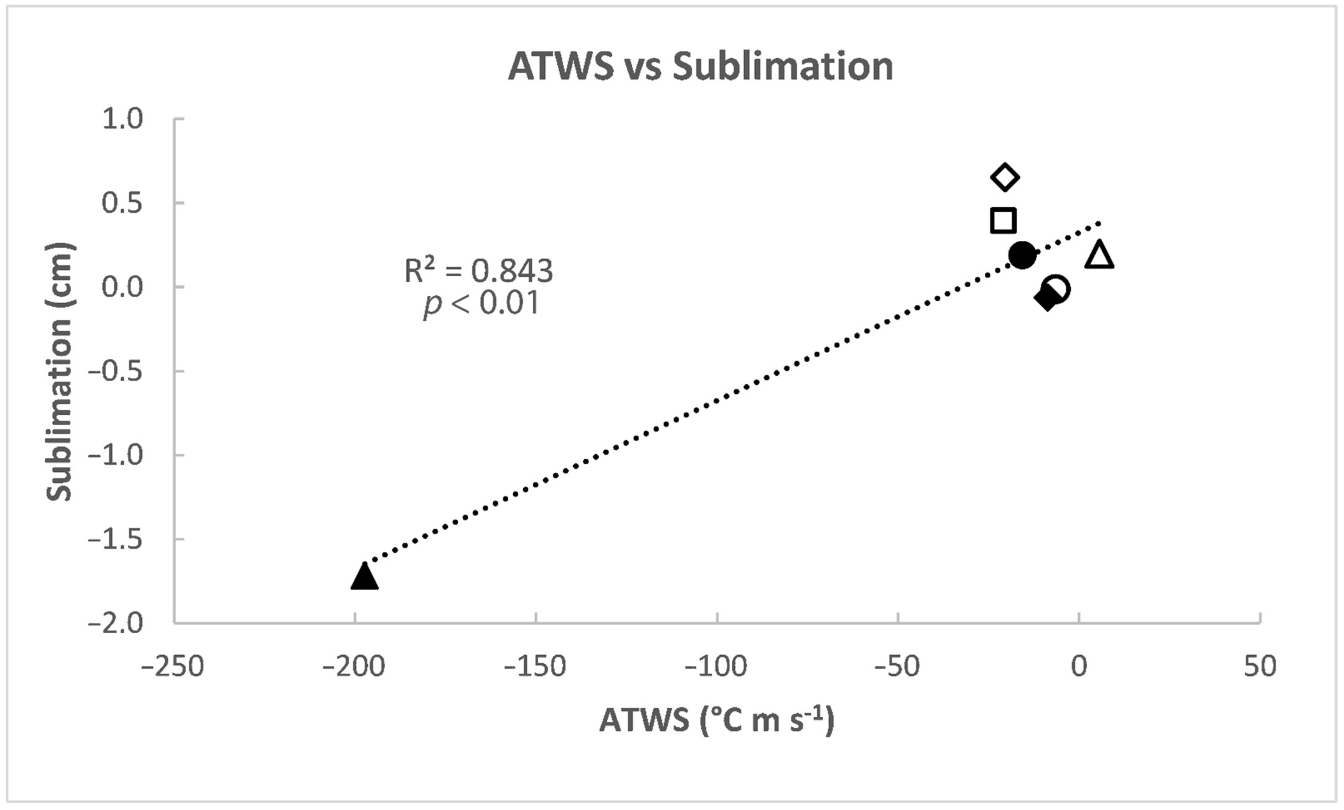
3.3. Sublimation
4. Discussion
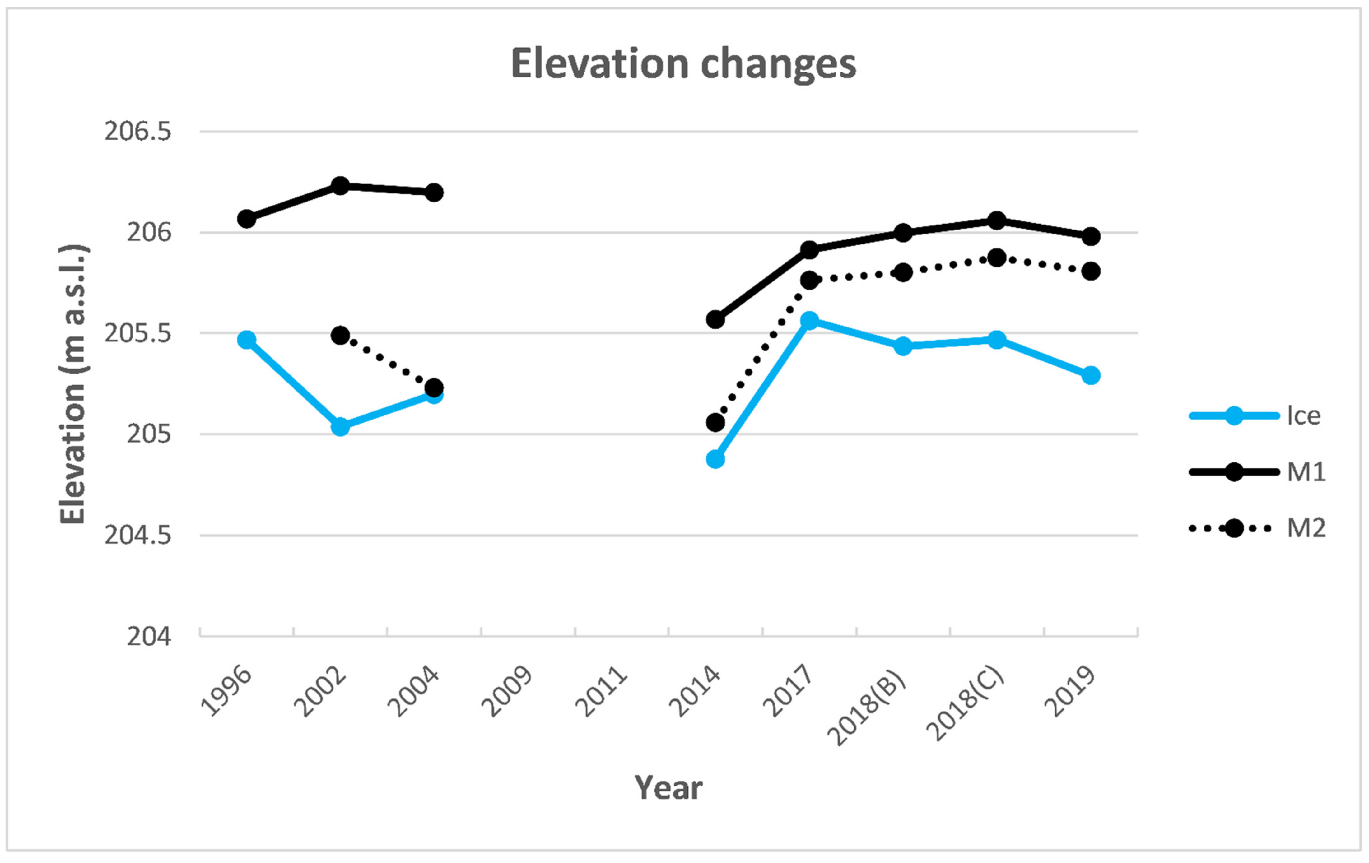
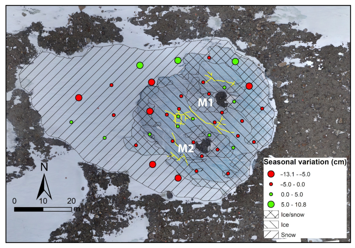
4.1. Frost Blisters and Lake Ice Surface Variations
4.2. Lake Ice and Snow Surface Sublimation
4.3. Water Recharge
5. Conclusions
Author Contributions
Funding
Institutional Review Board Statement
Informed Consent Statement
Data Availability Statement
Acknowledgments
Conflicts of Interest
References
- Kim, M.; Im, J.; Han, H.; Kim, J.; Lee, S.; Shin, M.; Kim, H.C. Landfast sea ice monitoring using multisensor fusion in the Antarctic. GISci. Remote Sens. 2015, 52, 239–256. [Google Scholar] [CrossRef]
- Lee, S.; Im, J.; Kim, J.; Kim, M.; Shin, M.; Kim, H.-C.; Quackenbush, L.J. Arctic Sea Ice Thickness Estimation from CryoSat-2 Satellite Data Using Machine Learning-Based Lead Detection. Remote Sens. 2016, 8, 698. [Google Scholar] [CrossRef] [Green Version]
- James, M.R.; Ilic, S.; Ruzic, I. Measuring 3D coastal change with a digital camera. Coast. Dyn. 2013, 893–904. [Google Scholar]
- Brunier, G.; Fleury, J.; Anthony, E.J.; Gardel, A.; Dussouillez, P. Close-range airborne Structure-from-Motion Photogrammetry for high-resolution beach morphometric surveys: Examples from an embayed rotating beach. Geomorphology 2016, 261, 76–88. [Google Scholar] [CrossRef]
- Li, T.; Zhang, B.; Cheng, X.; Westoby, M.J.; Li, Z.; Ma, C.; Hui, F.; Shokr, M.; Liu, Y.; Chen, Z.; et al. Resolving fine-scale surface features on polar sea ice: A first assessment of UAS photogrammetry without ground control. Remote Sens. 2019, 11, 784. [Google Scholar] [CrossRef] [Green Version]
- Zmarz, A.; Rodzewicz, M.; Dąbski, M.; Karsznia, I.; Korczak-Abshire, M.; Chwedorzewska, K.J. Application of UAV BVLOS remote sensing data for multi-faceted analysis of Antarctic ecosystem. Remote Sens. Environ. 2018, 217. [Google Scholar] [CrossRef]
- Lucieer, A.; Turner, D.; King, D.H.; Robinson, S.A. Using an unmanned aerial vehicle (UAV) to capture micro-topography of antarctic moss beds. Int. J. Appl. Earth Obs. Geoinf. 2014, 27. [Google Scholar] [CrossRef] [Green Version]
- Torrecillas, C.; Berrocoso, M.; Pérez-López, R.; Torrecillas, M.D. Determination of volumetric variations and coastal changes due to historical volcanic eruptions using historical maps and remote-sensing at Deception Island (West-Antarctica). Geomorphology 2012, 136. [Google Scholar] [CrossRef]
- Dąbski, M.; Zmarz, A.; Pabjanek, P.; Korczak-Abshire, M.; Karsznia, I.; Chwedorzewska, K.J. UAV-based detection and spatial analyses of periglacial landforms on Demay Point (King George Island, South Shetland Islands, Antarctica). Geomorphology 2017, 290. [Google Scholar] [CrossRef]
- Guglielmin, M.; Lewkowicz, A.G.; French, H.M.; Strini, A. Lake-ice blisters, terra nova bay area, Northern Victoria Land, antarctica. Geogr. Ann. Ser. A Phys. Geogr. 2009, 91. [Google Scholar] [CrossRef]
- French, H.M.; Guglielmin, M. Frozen ground phenomena in the vicinity of the Terra Nova bay, Northern Victoria land, Antarctica: A preliminary report. Geogr. Ann. Ser. A Phys. Geogr. 2000, 82. [Google Scholar] [CrossRef]
- Guglielmin, M.; Ponti, S.; Forte, E. The origins of Antarctic rock glaciers: Periglacial or glacial features? Earth Surf. Process. Landf. 2018, 43, 1390–1402. [Google Scholar] [CrossRef]
- Harris, S.A.; French, H.M.; Heginbottom, J.A.; Johnston, J.H.; Ladanyi, B.; Sego, D.C.; van Everdingen, R.O. Glossary of Permafrost and Related Ground-Ice Terms; National Research Council of Canada: Ottawa, ON, Canada, 1988. [Google Scholar]
- French, H.M. The Periglacial Environment, 4th ed.; Wiley: Hoboken, NJ, USA, 2017; 544p. [Google Scholar]
- Hinkel, K.M.; Peterson, K.M.; Eisner, W.R.; Nelson, F.E.; Turner, K.M.; Miller, L.L.; Outcalt, S.I. Formation of injection frost mounds over winter 1995–1996 at barrow, Alaska. Polar Geogr. 1996, 20. [Google Scholar] [CrossRef]
- Buteau, S.; Fortier, R.; Delisle, G.; Allard, M. Numerical simulation of the impacts of climate warming on a permafrost mound. Permafr. Periglac. Process. 2004, 15. [Google Scholar] [CrossRef]
- Pollard, W.H. Icing processes associated with high Arctic perennial springs, Axel Heiberg Island, Nunavut, Canada. Permafr. Periglac. Process. 2005, 16. [Google Scholar] [CrossRef]
- Morse, P.D.; Burn, C.R. Perennial frost blisters of the outer Mackenzie Delta, western Arctic coast, Canada. Earth Surf. Process. Landf. 2014, 39. [Google Scholar] [CrossRef]
- Van Autenboer, T. Ice Mounds and Melt Phenomena in the Sør-Rondane, Antarctica. J. Glaciol. 1962, 4. [Google Scholar] [CrossRef] [Green Version]
- Forte, E.; Dalle Fratte, M.; Azzaro, M.; Guglielmin, M. Pressurized brines in continental Antarctica as a possible analogue of Mars. Sci. Rep. 2016, 6. [Google Scholar] [CrossRef] [Green Version]
- Pollard, W.H. Seasonal frost mounds. Can. Geogr. 1991, 35. [Google Scholar] [CrossRef]
- Hagedorn, B.; Sletten, R.S.; Hallet, B.; McTigue, D.F.; Steig, E.J. Ground ice recharge via brine transport in frozen soils of Victoria Valley, Antarctica: Insights from modeling δ18O and δD profiles. Geochim. Cosmochim. Acta 2010, 74. [Google Scholar] [CrossRef]
- Levy, J.S.; Fountain, A.G.; Gooseff, M.N.; Welch, K.A.; Lyons, W.B. Water tracks and permafrost in Taylor Valley, Antarctica: Extensive and shallow groundwater connectivity in a cold desert ecosystem. Bull. Geol. Soc. Am. 2011, 123. [Google Scholar] [CrossRef]
- Gooseff, M.N.; Barrett, J.E.; Levy, J.S. Shallow groundwater systems in a polar desert, McMurdo Dry Valleys, Antarctica. Hydrogeol. J. 2013, 21. [Google Scholar] [CrossRef]
- Dugan, H.A.; Doran, P.T.; Tulaczyk, S.; Mikucki, J.A.; Arcone, S.A.; Auken, E.; Schamper, C.; Virginia, R.A. Subsurface imaging reveals a confined aquifer beneath an ice-sealed Antarctic lake. Geophys. Res. Lett. 2015, 42. [Google Scholar] [CrossRef]
- Dugan, H.A.; Obryk, M.K.; Doran, P.T. Lake ice ablation rates from permanently ice-covered Antarctic lakes. J. Glaciol. 2013, 59. [Google Scholar] [CrossRef] [Green Version]
- Van Everdingen, R.O. Frost Blisters of the Bear Rock Spring Area near Fort Norman, N.W.T. Arctic 1982, 35. [Google Scholar] [CrossRef] [Green Version]
- Beck, I.; Ludwig, R.; Bernier, M.; Strozzi, T.; Boike, J. Vertical movements of frost mounds in subarctic permafrost regions analyzed using geodetic survey and satellite interferometry. Earth Surf. Dyn. 2015, 3. [Google Scholar] [CrossRef] [Green Version]
- Pollard, W.H.; French, H.M. The groundwater hydraulics of seasonal frost mounds, North Fork Pass, Yukon Territory. Can. J. Earth Sci. 1984. [Google Scholar] [CrossRef]
- Walvoord, M.A.; Voss, C.I.; Wellman, T.P. Influence of permafrost distribution on groundwater flow in the context of climate-driven permafrost thaw: Example from Yukon Flats Basin, Alaska, United States. Water Resour. Res. 2012, 21. [Google Scholar] [CrossRef]
- Doran, P.T.; McKay, C.P.; Fountain, A.G.; Nylen, T.; McKnight, D.M.; Jaros, C.; Barrett, J.E. Hydrologic response to extreme warm and cold summers in the McMurdo Dry Valleys, East Antarctica. Antarct. Sci. 2008, 20. [Google Scholar] [CrossRef] [Green Version]
- Scarchilli, C.; Frezzotti, M.; Grigioni, P.; De Silvestri, L.; Agnoletto, L.; Dolci, S. Extraordinary blowing snow transport events in East Antarctica. Clim. Dyn. 2010, 34. [Google Scholar] [CrossRef] [Green Version]
- Andersen, D.T.; McKay, C.P.; Lagun, V. Climate conditions at perennially ice-covered lake Untersee, East Antarctica. J. Appl. Meteorol. Climatol. 2015, 54. [Google Scholar] [CrossRef]
- Faucher, B.; Lacelle, D.; Fisher, D.A.; Andersen, D.T.; McKay, C.P. Energy and water mass balance of Lake Untersee and its perennial ice cover, East Antarctica. Antarct. Sci. 2019, 31. [Google Scholar] [CrossRef]
- Gooseff, M.N.; McKnight, D.M.; Doran, P.; Fountain, A.G.; Lyons, W.B. Hydrological connectivity of the landscape of the McMurdo Dry Valleys, Antarctica. Geogr. Compass 2011, 5. [Google Scholar] [CrossRef]
- Scheidegger, J.M.; Bense, V.F. Impacts of glacially recharged groundwater flow systems on talik evolution. J. Geophys. Res. Earth Surf. 2014. [Google Scholar] [CrossRef]
- Ge, S.; McKenzie, J.; Voss, C.; Wu, Q. Exchange of groundwater and surface-water mediated by permafrost response to seasonal and long term air temperature variation. Geophys. Res. Lett. 2011, 119. [Google Scholar] [CrossRef] [Green Version]
- Wellman, T.P.; Voss, C.I.; Walvoord, M.A. Impacts of climate, lake size, and supra- and sub-permafrost groundwater flow on lake-talik evolution, Yukon Flats, Alaska (USA). Hydrogeol. J. 2013, 21. [Google Scholar] [CrossRef]
- Sannino, C.; Borruso, L.; Mezzasoma, A.; Battistel, D.; Zucconi, L.; Selbmann, L.; Azzaro, M.; Onofri, S.; Turchetti, B.; Buzzini, P.; et al. Intra- and inter-cores fungal diversity suggests interconnection of different habitats in an Antarctic frozen lake (Boulder Clay, Northern Victoria Land). Environ. Microbiol. 2020, 22. [Google Scholar] [CrossRef]
- Rizzo, C.; Conte, A.; Azzaro, M.; Papale, M.; Rappazzo, A.C.; Battistel, D.; Roman, M.; Giudice, A.L.; Guglielmin, M. Cultivable bacterial communities in brines from perennially icecovered and pristine antarctic lakes: Ecological and biotechnological implications. Microorganisms 2020, 8, 819. [Google Scholar] [CrossRef]
- Monaghan, A.J.; Bromwich, D.H.; Fogt, R.L.; Wang, S.H.; Mayewski, P.A.; Dixon, D.A.; Ekaykin, A.; Frezzotti, M.; Goodwin, I.; Isaksson, E.; et al. Insignificant change in Antarctic snowfall since the international geophysical year. Science 2006, 313. [Google Scholar] [CrossRef] [Green Version]
- Guglielmin, M.; Dalle Fratte, M.; Cannone, N. Permafrost warming and vegetation changes in continental Antarctica. Environ. Res. Lett. 2014, 9. [Google Scholar] [CrossRef] [Green Version]
- Guglielmin, M.; Biasini, A.; Smiraglia, C. The contribution of geoelectrical investigations in the analysis of periglacial and glacial landforms in ice free areas of the Northern Foothills (Northern Victoria Land, Antarctica). Geogr. Ann. Ser. A Phys. Geogr. 1997, 79. [Google Scholar] [CrossRef]
- Cannone, N.; Wagner, D.; Hubberten, H.W.; Guglielmin, M. Biotic and abiotic factors influencing soil properties across a latitudinal gradient in Victoria Land, Antarctica. Geoderma 2008, 144. [Google Scholar] [CrossRef] [Green Version]
- Guglielmin, M. Ground surface temperature (GST), active layer and permafrost monitoring in continental Antarctica. Permafr. Periglac. Process. 2006, 17. [Google Scholar] [CrossRef]
- French, H.M.; Guglielmin, M. Observations on the ice-marginal, periglacial geomorphology of Terra Nova Bay, Northern Victoria Land, Antarctica. Permafr. Periglac. Process. 1999, 10. [Google Scholar] [CrossRef]
- Molau, U.; Mølgaard, P. ITEX; Danish Polar Center: Copenhagen, Denmark, 1996. [Google Scholar]
- Doran, P.T.; Mckay, C.P.; Meyer, M.A.; Andersen, D.T.; Wharton, R.A.; Hastings, J.T. Climatology and implications for perennial lake ice occurrence at Bunger Hills Oasis, East Antarctica. Antarct. Sci. 1996, 8. [Google Scholar] [CrossRef]
- James, M.R.; Robson, S. Straightforward reconstruction of 3D surfaces and topography with a camera: Accuracy and geoscience application. J. Geophys. Res. Earth Surf. 2012, 117. [Google Scholar] [CrossRef] [Green Version]
- Uysal, M.; Toprak, A.S.; Polat, N. DEM generation with UAV Photogrammetry and accuracy analysis in Sahitler hill. Meas. J. Int. Meas. Confed. 2015, 73. [Google Scholar] [CrossRef]
- Chandler, J. Effective application of automated digital photogrammetry for geomorphological research. Earth Surf. Process. Landf. 1999, 24. [Google Scholar] [CrossRef]
- Milan, D.J.; Heritage, G.L.; Hetherington, D. Application of a 3D laser scanner in the assessment of erosion and deposition volumes and channel change in a proglacial river. Earth Surface Process. Landf. 2007, 32, 1657–1674. [Google Scholar] [CrossRef]
- Brasington, J.; Langham, J.; Rumsby, B. Methodological sensitivity of morphometric estimates of coarse fluvial sediment transport. Geomorphology 2003, 53. [Google Scholar] [CrossRef]
- Hagedorn, B.; Sletten, R.S.; Hallet, B. Sublimation and ice condensation in hyperarid soils: Modeling results using field data from Victoria Valley, Antarctica. J. Geophys. Res. Earth Surf. 2007, 112. [Google Scholar] [CrossRef] [Green Version]
- Bliss, A.K.; Cuffey, K.M.; Kavanaugh, J.L. Sublimation and surface energy budget of Taylor Glacier, Antarctica. J. Glaciol. 2011, 57. [Google Scholar] [CrossRef] [Green Version]
- Clow, G.D.; McKay, C.P.; Simmons, G.M.; Wharton, R.A. Climatological observations and predicted sublimation rates at Lake Hoare, Antarctica. J. Clim. 1988, 1. [Google Scholar] [CrossRef] [Green Version]
- Bintanja, R. The contribution of snowdrift sublimation to the surface mass balance of Antarctica. Ann. Glaciol. 1998, 27. [Google Scholar] [CrossRef] [Green Version]
- Bintanja, R. On the glaciological, meteorological, and climatological significance of Antarctic blue ice areas. Rev. Geophys. 1999, 37. [Google Scholar] [CrossRef]
- Doran, P.T.; Wharton, R.A.; Lyons, W.B. Paleolimnology of the McMurdo Dry Valleys, Antarctica. J. Paleolimnol. 1994, 10. [Google Scholar] [CrossRef]
- Chinn, T.J. Physical hydrology of the dry valley lakes. In Physical and Biogeochemical Processes in Antarctic Lakes; Green, W.J., Friedmann, I.E., Eds.; American Geophysical Union: Washington, DC, USA, 1993; Volume 59, pp. 1–51. [Google Scholar]
- Liu, L.; Sletten, R.S.; Hagedorn, B.; Hallet, B.; McKay, C.P.; Stone, J.O. An enhanced model of the contemporary and long-term (200 ka) sublimation of the massive subsurface ice in Beacon Valley, Antarctica. J. Geophys. Res. F Earth Surf. 2015, 120. [Google Scholar] [CrossRef]
- Albert, M.R. Effects of snow and firm ventilation on sublimation rates. Ann. Glaciol. 2002, 35. [Google Scholar] [CrossRef]
- La Ferla, R.; Azzaro, M.; Michaud, L.; Caruso, G.; Lo Giudice, A.; Paranhos, R.; Cabral, A.S.; Conte, A.; Cosenza, A.; Maimone, G.; et al. Prokaryotic Abundance and Activity in Permafrost of the Northern Victoria Land and Upper Victoria Valley (Antarctica). Microb. Ecol. 2017, 74. [Google Scholar] [CrossRef]
- Guglielmin, M.; French, H.M. Ground ice in the Northern Foothills, northern Victoria Land, Antarctica. Ann. Glaciol. 2004, 39. [Google Scholar] [CrossRef]
- Brandt, R.E.; Warren, S.G. Solar-heating rates and temperature profiles in Antarctic snow and ice. J. Glaciol. 1993, 39. [Google Scholar] [CrossRef] [Green Version]
- Guglielmin, M.; Cannone, N. A permafrost warming in a cooling Antarctica? Clim. Chang. 2012, 111. [Google Scholar] [CrossRef]


| Survey | Date | Camera | Markers | GCPs | Check Points | Resolution (cm) | Reprojection Error of Tie Points (px) | Reprojection Error of Markers (px) | Vertical Error of Check Points (cm) |
|---|---|---|---|---|---|---|---|---|---|
| A | 08/11/2017 | Honor 9 Smartphone—20 MP | 9 | 5 | 1 | 8.1 | 1.0–3.6 | 1.8–3.2 | 2.3 |
| B | 03/12/2018 | Sony QX1—20 MP | 21 | 13 | 7 | 0.7 | 0.3–1.0 | 0.3–0.6 | 2.0 |
| C | 30/12/2018 | Sony QX1—20 MP | 20 | 13 | 3 | 0.6 | 0.3–1.5 | 0.2–1.0 | 1.0 |
| D | 21/11/2019 | Sony QX1—20 MP | 15 | 12 | 3 | 0.7 | 0.5–0.9 | 0.3–0.9 | 1.5 |
| Mean Elevation from Pixel Analysis (m a.s.l.) | Mean Elevation from DEM (m a.s.l.) | Area (m2) | Volume (m3) | |||||||
|---|---|---|---|---|---|---|---|---|---|---|
| M1 | M2 | Ice | M1 | M2 | Ice | M1 | M2 | M1 | M2 | |
| 1996 | 206.067 | 205.468 | ||||||||
| 2002 | 206.231 | 205.489 | 205.036 | |||||||
| 2004 | 206.198 | 205.229 | 205.196 | 32.0 | 21.3 | |||||
| 2009 | 19.6 | 0 | ||||||||
| 2011 | 15.9 | 1 | ||||||||
| 2014 | 205.569 | 205.058 | 204.878 | 18.2 | 16.3 | |||||
| 2017 (A) | 205.913 | 205.762 | 205.563 | 1.93 | 0.95 | |||||
| 2018 (B) | 205.997 | 205.801 | 205.435 | 20.7 | 23.6 | 2.35 | 1.24 | |||
| 2018 (C) | 206.058 | 205.874 | 205.468 | 2.76 | 1.49 | |||||
| 2019 (D) | 205.98 | 205.807 | 205.29 | 22.3 | 21.5 | 2.35 | 1.17 | |||
| Area (%) | Mean Change (cm) | St. Dev. (cm) | Accuracy (cm) | |||||
|---|---|---|---|---|---|---|---|---|
| 2018 | 2019 | 2018 | 2019 | 2018 | 2019 | 2018 | 2019 | |
| Ice | 21.9 | 48.7 | 3.6 | −18.1 | 2.5 | 6.1 | 4.4 | 3.5 |
| Snow | 51.3 | 51.3 | 14.9 | −12.3 | 8.9 | 9.2 | ||
| Ice/Snow | 26.8 | - | 8.6 | - | 5.2 | - | ||
| Min (cm) | Max (cm) | Mean (cm) | St. Dev. (cm) | |
|---|---|---|---|---|
| Ice | −4.3 | 3.4 | −0.7 | 1.7 |
| Snow | −12.0 | 10.8 | −2.0 | 8.6 |
| Ice/Snow | −13.1 | 7.9 | −2.4 | 5.3 |
Publisher’s Note: MDPI stays neutral with regard to jurisdictional claims in published maps and institutional affiliations. |
© 2021 by the authors. Licensee MDPI, Basel, Switzerland. This article is an open access article distributed under the terms and conditions of the Creative Commons Attribution (CC BY) license (http://creativecommons.org/licenses/by/4.0/).
Share and Cite
Ponti, S.; Scipinotti, R.; Pierattini, S.; Guglielmin, M. The Spatio-Temporal Variability of Frost Blisters in a Perennial Frozen Lake along the Antarctic Coast as Indicator of the Groundwater Supply. Remote Sens. 2021, 13, 435. https://0-doi-org.brum.beds.ac.uk/10.3390/rs13030435
Ponti S, Scipinotti R, Pierattini S, Guglielmin M. The Spatio-Temporal Variability of Frost Blisters in a Perennial Frozen Lake along the Antarctic Coast as Indicator of the Groundwater Supply. Remote Sensing. 2021; 13(3):435. https://0-doi-org.brum.beds.ac.uk/10.3390/rs13030435
Chicago/Turabian StylePonti, Stefano, Riccardo Scipinotti, Samuele Pierattini, and Mauro Guglielmin. 2021. "The Spatio-Temporal Variability of Frost Blisters in a Perennial Frozen Lake along the Antarctic Coast as Indicator of the Groundwater Supply" Remote Sensing 13, no. 3: 435. https://0-doi-org.brum.beds.ac.uk/10.3390/rs13030435