Variations of Water Transparency and Impact Factors in the Bohai and Yellow Seas from Satellite Observations

Abstract

Water transparency, measured with Secchi disk depth (SDD), is an important parameter for describing the optical properties of a water body. This study evaluates variations of SDD and related impact factors in the Bohai and Yellow Seas (BYS). Based on a new mechanistic model proposed by Lee et al. (2015) applied to MODIS remote sensing reflectance data, climatological SDD variation from 2003 to 2019 was estimated. The annual mean images showed an increasing trend from the coastal zone to the deep ocean. Lower values were found in the Bohai Sea (BHS), while higher values observed in the center of the southern Yellow Sea (SYS). Additionally, the entire sea has shown a decreasing temporal tend, with the variation rate lowest in the BHS at 0.003 m y⁻¹, and highest in the SYS at 0.015 m y⁻¹. However, the weak increasing trend that appeared since 2017 suggests that water quality seems to have improved. Further, it displayed seasonal patterns of low in winter and spring and high in summer and autumn. The empirical orthogonal function (EOF) analysis of SDD variations over the BYS, shows that the first SDD EOF mode is the highest, strongly correlated with total suspended matter. With the high correlation coefficients of chromophoric dissolved organic matter, it illustrates that the SDD variation is mainly dominated by the optical components in the seawater, although correlation with chlorophyll-a is the weakest. The second and third EOF modes show that photosynthetically available radiation, sea surface temperature, sea surface salinity, and wind speed are the main covariates that cause SDD changes. Water transparency evaluation on a long-term scale is essential for water quality monitoring and marine ecosystem protection.

1. Introduction

In marine and lake ecosystems, the penetration and availability of light underwater is a controlling factor of the physical (sediment suspension and heat transfer), biological (phytoplankton photosynthesis), and chemical (cycling of nutrients) processes of the water body [1]. Therefore, water transparency is a key parameter for describing the optical properties in the water body. Water transparency is closely related to many environmental parameters, such as chlorophyll-a (Chl-a) [2,3,4], phytoplankton biomass [5], total suspended matter (TSM) [6], nutritional status [7], sea surface salinity [8], total nitrogen and total phosphorus [9], and widely used as evaluation indicators of marine environmental quality [10].

The Bohai and Yellow Seas (BYS) are located in the northwestern margin of the Pacific Ocean [11]. The sea area has a complex hydrodynamic environment, and also affected by a large amount of freshwater and sediments from the surrounding two world-famous rivers (the Yellow River and the Yangtze River). The marine community is rich and diverse, with clear seasonal changes of water optical properties. Due to the complexity of the optical properties and the importance of the marine ecological environment, it is desired to obtain the long-term monitoring data of water transparency and establish its relationship with environmental factors in the BYS, to improve the understanding of the dynamic variations of marine ecosystems in the region.

For the in situ water transparency measurement, the Secchi disk, which is the oldest “optical instrument” and dates from 1865, is a simple, fast, and low-cost commonly used tool [12]. The Secchi disk depth (SDD) is the depth when a black and white Secchi disk disappears from the observer’s sight in the human eye when it is deployed into the water [13] and is considered to be a reasonable estimate of water transparency at visible light range [14]. Due to the limitations of a ship survey, the measured data can be discrete and sparse in time and space, and poorly synchronized, which can affect the detailed and objective evaluation of the variation of water transparency. As proved in the past few decades, the satellite sensors with repeated measurements of the same sea area can offer a wealth of ocean information, and improve the spatial and temporal coverage of environmental monitoring. It has been an important source of information for assessing global and regional aquatic environment conditions and trends [15,16,17]. On-board ocean color sensors have been successfully used to monitor SDD, such as the Moderate Resolution Image Spectroradiometer (MODIS) [18,19,20].

In previous studies, the water transparency estimation using remote sensing approaches were mainly applied to inland water in China [21,22,23] with few reports on the coastal and marine regions of China seas. For example, the Bohai Sea (BHS) was found to have the lowest water transparency among the East China Seas from in situ collected data over a 21-year period (1959–1979) [24]. Considering the residual error in satellite remote sensing reflectance (R_rs) data, an SDD empirical retrieval model coupled with a band difference method was developed for China Eastern Coastal Zone and shows that increasingly more waters within 30–35 and 20–25 m isobaths were deteriorating from 2002 to 2014 [25]. For the central BHS, accompanying rapid economic growth at the end of the 1980s, there was a significant decrease in the water quality, but no significant variations were detected between 2003 and 2014 [26]. Using a regionally tuned model from the Geostationary Ocean Color Imager (GOCI) data over the BYS, the water transparency shows obvious temporal variations, the daily change is primarily driven by the changes in the solar zenith angle, and the monthly variation is mainly driven by the stability of the water body stratification [27]. However, the main driving force of the long-term SDD changes in the BYS has not yet been evaluated and analyzed in detail.

Therefore, this study applied the new mechanistic model from Lee et al. (2015) [28] to MODIS R_rs data from 2003 to 2019 in order to explore the SDD changes in the BYS. Marine environmental factors, including near-surface Chl-a concentration, TSM concentration, chromophoric dissolved organic matter (CDOM) concentration, sea surface temperature (SST), photosynthetically available radiation (PAR), sea surface salinity (SSS), and wind vectors were assessed for the study region using satellite observations. Therefore, the aims of this study are to (1) use long-term MODIS R_rs monthly mean products to estimate the SDD values of the BYS from SDD algorithm of Lee et al. (2015), and analyze the spatial distribution and temporal variation trend of SDD from 2003 to 2019; (2) carry out statistical analysis between the main components from the EOF decomposition and the environmental factors that affect SDD changes, and clarify the main impact factors of SDD changes in the BYS; and (3) elucidate the water components and marine environmental factors for the driving mechanism of SDD changes.

2. Data and Methods

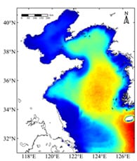
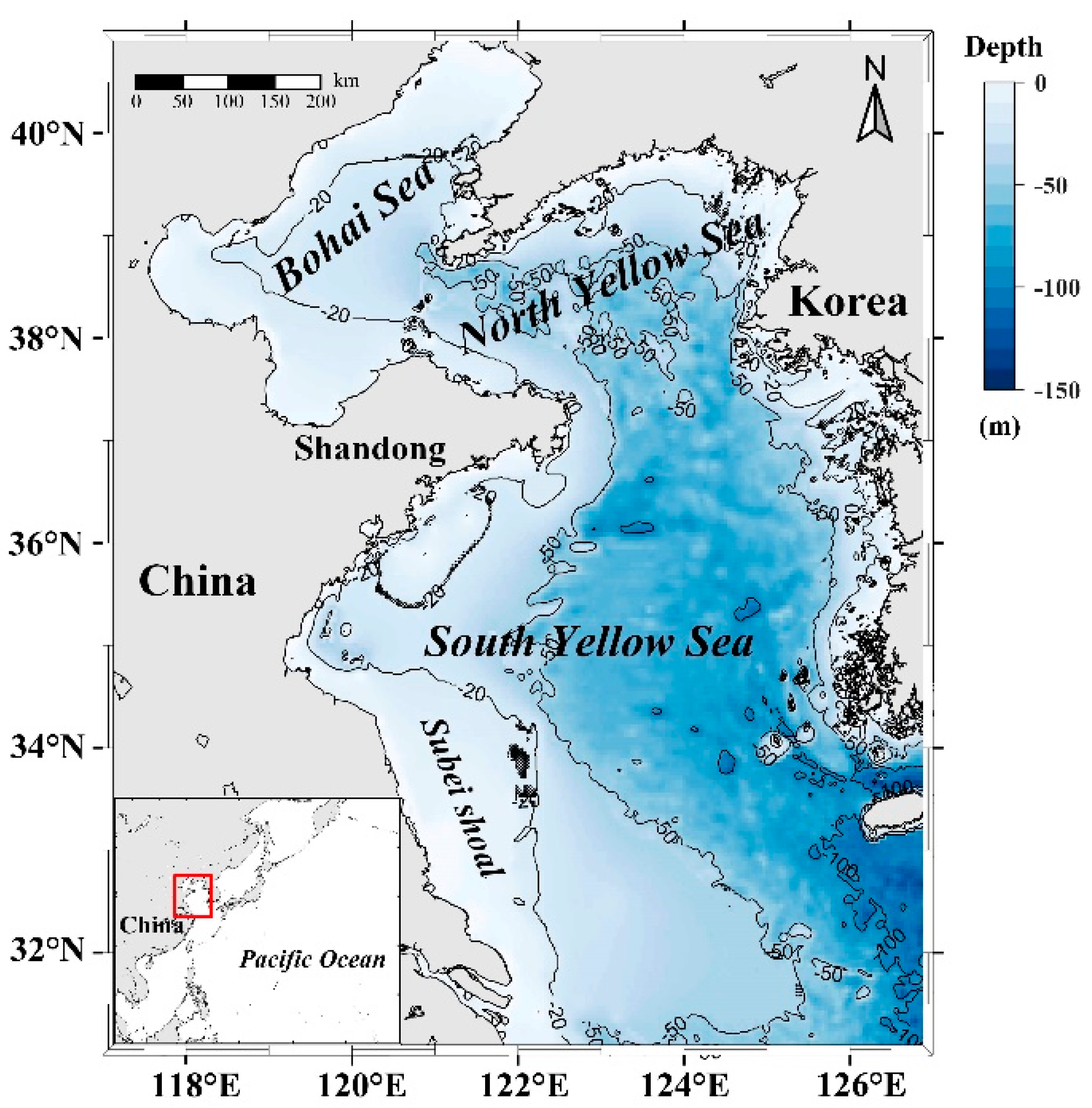
2.1. Study Area

The Bohai and Yellow Seas (31°–41°N, 117°–127°E) are semiclosed continental shelf shallow seas, with depths generally less than 100 m [29], as shown in Figure 1. The Bohai Sea is a shallow shelf basin covering 7.70×10⁴ km² and an average water depth of 18 m [30]. The Yellow Sea (YS) is contiguous to the Bohai Sea through the Bohai Strait with an average water depth of about 44 m and coverage of 3.8×10⁵ km² [31]. Affected by the East Asian monsoon, a north wind prevails in winter, and the average wind speed is about 8–9 m s⁻¹. The high-salt tongue penetrates the northern part of the Yellow Sea and enters the Bohai Sea via the Bohai Strait. The circulation is largely affected by the sea surface wind and brings strong vertical mixing in the water body [32]. The south wind prevails in summer with an average wind speed of 4–6 m s⁻¹, resulting in low surface salinity in the YS. Most areas of the Yellow Sea are regulated by the semidiurnal tide, which is the main driving force of the Bohai Sea environment [33].

2.2. Remote Sensing Data

2.2.1. NASA Ocean Color Data

Monthly Level 3 standard mapped image of R_rs at 412, 443, 469, 488, 531, 555, 660, 680, and 745 nm, taken at a spatial resolution of 4 km × 4 km, were acquired from MODIS-Aqua between January 2003 and December 2019. The data were downloaded from the National Aeronautics and Space Administration (NASA) Ocean Biology Distributed Active Archive Center (https://oceancolor.gsfc.nasa.gov/l3/). Meanwhile, sea surface Chl-a concentration, TSM concentration, and photosynthetically available radiation (PAR) calculated from monthly mean R_rs data were obtained for establishing the relationship with water transparency variations. Chl-a concentrations were calculated using the standard OC3/OC4 (OCx) blue-to-green band ratio algorithm [34] combined with the Hu color index algorithm [35]. The TSM concentration was taken by applying the algorithm constructed in Zhang et al. (2010) [36]. The PAR is derived from the solar energy at the top of the atmosphere that removed the ocean–atmosphere system reflection and the atmosphere absorption, and commonly related to marine primary productivity [37]. CDOM concentration represented by CDOM absorption coefficients at 440 nm (a_CDOM(440)) can be separated from absorption coefficients of CDOM and nonalgal particles based on the QAA_CDOM algorithm [38,39].

2.2.2. GHRSST Products

The daily gridded AVHRR SST data at 4 km × 4 km spatial resolution were provided by the Group for High-Resolution Sea Surface Temperature (GHRSST, https://data.nodc.noaa.gov/ghrsst/L3C/) [40,41]. Monthly mean SST time series data were composited from daily averaged SST data from January 2003 to December 2019.

2.2.3. RMESS Products

The wind vector data near the ocean surface (including wind speed and wind direction) were derived from Quick Scatterometer (QuikSCAT) and the first Advanced Scatterometer (ASCAT) of Remote Sensing Systems (RSS, http://www.remss.com/). Compared with QuikSCAT, ASCAT data shows a high level of consistency at all wind speed regimes by using a similar methodology and wind algorithm [42,43]. Monthly gridded data of wind vectors from January 2003 to November 2009 were derived from QuikSCAT, and data from March 2007 and December 2019 were obtained from ASCAT. For products with the same month in both datasets, the specified variables were averaged in the data grid to generate monthly average fusion data.

2.2.4. CMEMS Dataset

SSS data were taken from the European Copernicus Marine Environment Monitoring Service (CMEMS, https://marine.copernicus.eu/). Global ocean multiobservation reanalysis products in the framework of CMEMS operationally provide dynamics information of the ocean and marine ecosystems and rely on in situ measured networks to calibrate and validate the data from satellites [44]. The SSS L4 dataset was obtained by a multidimensional optimal interpolation technique from interpolating in situ and satellite-derived SSS data [45]. The grid data were resampled to 4 km × 4 km resolution from the raw spatial resolution of 0.25° × 0.25° (about 25 km × 25 km).

2.3. Methods

2.3.1. Algorithm to Retrieve SDD

Based on classical underwater visibility theory, an analytical model for SDD retrieval has been developed [46], but the modeled data are not in agreement with in situ measurements. To exactly interpret the physical processes of sighting a Secchi disk in water by the human eye, a new underwater visibility theory described by Lee et al. (2015) was then proposed and an innovative mechanistic model for SDD was established. Using this model to retrieve water transparency, it mainly includes three main steps. First, the quasi-analytical algorithm (QAA) is used to estimate the total absorption coefficient a(λ) and the total scattering coefficient b_b(λ) of the water from R_rs(λ) data [47]. If R_rs(670) is less than 0.0015 sr⁻¹, the reference band is taken 550 nm, otherwise, 670 nm is selected. Second, according to the model developed by Lee et al. (2005, 2013) [48,49], the diffuse attenuation coefficient K_d(λ) is evaluated as follows:

$${\mathrm{K}}_{\mathrm{d}}(\lambda )=(1+{\mathrm{m}}_0\times {\mathrm{\theta }}_{\mathrm{s}})\times \mathrm{a}(\lambda )+{\mathrm{m}}_1\times (1-\gamma \times {\eta }_w(\mathrm{\lambda }))\times (1\mathrm{-}{\mathrm{m}}_2\times {\mathrm{e}}^{-{\mathrm{m}}_3\times \mathrm{a}(\mathrm{\lambda })})\times {\mathrm{b}}_{\mathrm{b}}(\mathrm{\lambda }),$$

(1)

Here, the four parameters m_0-3 that vary with solar altitudes and depth owing to the change of light distribution are queried through a lookup table. The variable θ_s is the solar zenith angle and η_w is the ratio of the pure seawater backscattering coefficient b_bw(λ) to b_b(λ). The pure seawater coefficients of absorption and backscattering at each wavelength were tabulated by Morel [50] and Smith and Baker [51]. Finally, following this new underwater visibility theory [28], SDD is given by

$$\mathrm{SDD}=\frac{1}{2.5\mathrm{Min}({\mathrm{K}}_{\mathrm{d}}(\mathrm{\lambda }))}\ln (\frac{\left|0.14-{\mathrm{R}}_{\mathrm{r}\mathrm{s}}{}^{\mathrm{P}\mathrm{C}}\right|}{{\mathrm{C}}_{\mathrm{t}}{}^{\mathrm{r}}}),$$

(2)

where Min(K_d(λ)) is the minimum K_d value in the visible domain wavelength of MODIS, R_rs^PC is the R_rs value matched to the wavelength with minimum K_d, and C_t^r is the contrast threshold for human eyes to sight a Secchi disk and taken as an average of 0.013 sr⁻¹ based on the measurements of Blackwell (1946) [52]. For global combined in situ datasets of 338 R_rs and SDD matchup with SDD range of 0.1 m to 30 m, which contains 197 pairs of matching points from field measurements off China Seas, the accuracy of the new model was statistically verified. The mean absolute relative difference between measured and model retrieved SDD is 18.2%, and this difference includes 10% or more uncertainties in the observation of Secchi disk depth.

2.3.2. Trend Analysis

To evaluate the temporal variation of water transparency, the Mann–Kendall (MK) test was carried out to evaluate the temporal changes and significance of trends. Meanwhile, Sen’s slope (SS) was used to obtain the magnitude of variation [53]. The combination of both methods has been extensively used for trend analysis in hydrometeorological time series. In the MK test, the Z score obeys the standard normal distribution. When its absolute value is greater than 1.96, the evaluated trends are significant at 5% significance level [54]; it can be used to estimate the significance of the variation trend.

Regression analysis was used to evaluate the quantitative relationship between dependent and independent variables. For the single variable linear regression of the observed factors for time, the linear trend can be obtained from the least square fitting [55]. Before the regression was applied, all assumptions of the analysis (i.e., normality, homoscedasticity, and independence of predictor variables) were tested and met. Specifically, we used this test to verify that there was no autocorrelation between predictor variables.

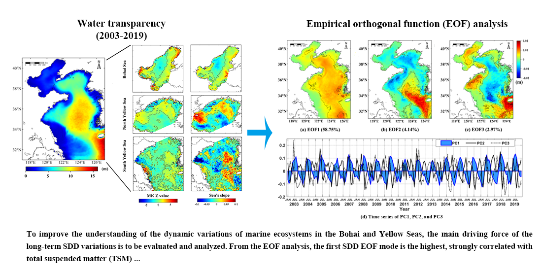
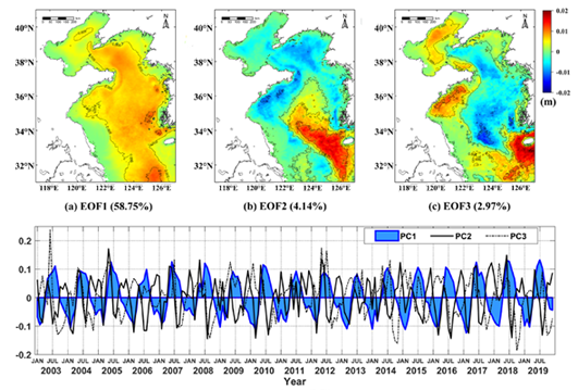
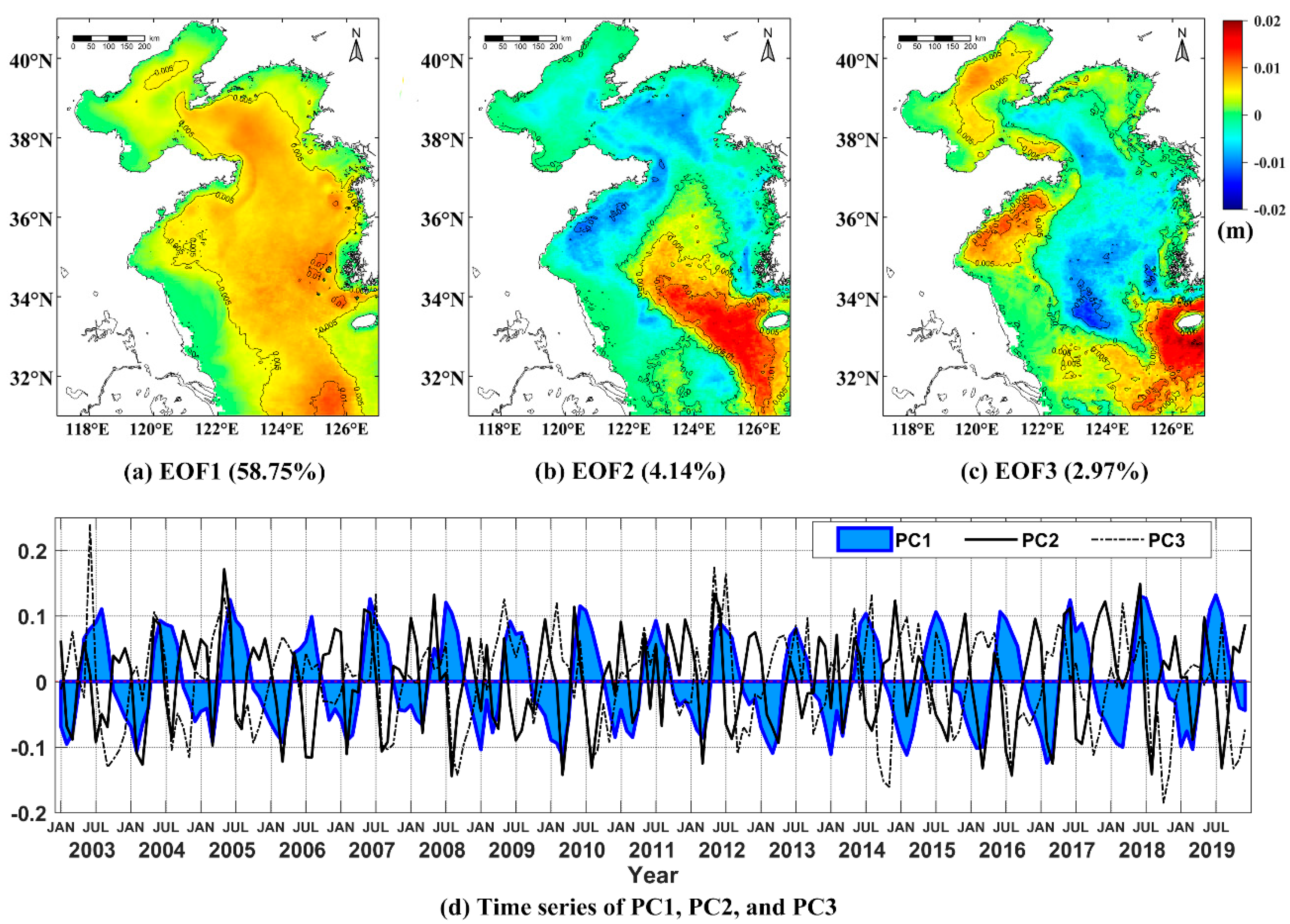
2.3.3. Empirical Orthogonal Function Decomposition

The empirical orthogonal function (EOF) is a principal component analysis (PCA) method that was first introduced into meteorology and climate research by Lorenz in the 1950s [56], and now it has been widely used in the field of oceanography [57]. In general, the eigenvector corresponds to the spatial sample, so called the spatial mode (hereafter referred to as EOFs); the principal components (PCs) correspond to the time change. It can identify key variability patterns from the time series data of the spatial map. When a certain pattern can be statistically related to different physical processes, this allows for the underlying driving mechanisms to be evaluated.

When EOF decomposition is applied to the special parameters observation, the long time series data over spatial gridded points should be taken for anomaly processing first. Then, the eigenvalues and eigenvectors can be calculated easily using singular value decomposition (SVD) techniques to substitute for the classical covariance matrix approach to save the entire computational time. Arranging the eigenvalues in descending order, a list of eigenvectors corresponding to each nonzero eigenvalue is taken as a spatial distribution mode. The temporal mode can be found by multiplying the eigenvectors with the transpose of the original matrix. The size of the eigenvalue determines the contribution of the corresponding eigenvector to the total variance. The first EOF mode represents the long-term trend of time series changes, while higher-order EOF harmonics are detrended. At last, the North test is chosen to test the significance of the error range of the eigenvalue and judge whether the result of decomposition is meaningless noise or a signal with physical significance [58]. It is worth noting that since each independent variability pattern is spatially dependent, the EOF analysis results would rely on the spatial area of the data grid involved.

3. Results

3.1. Spatial and Temporal Patterns

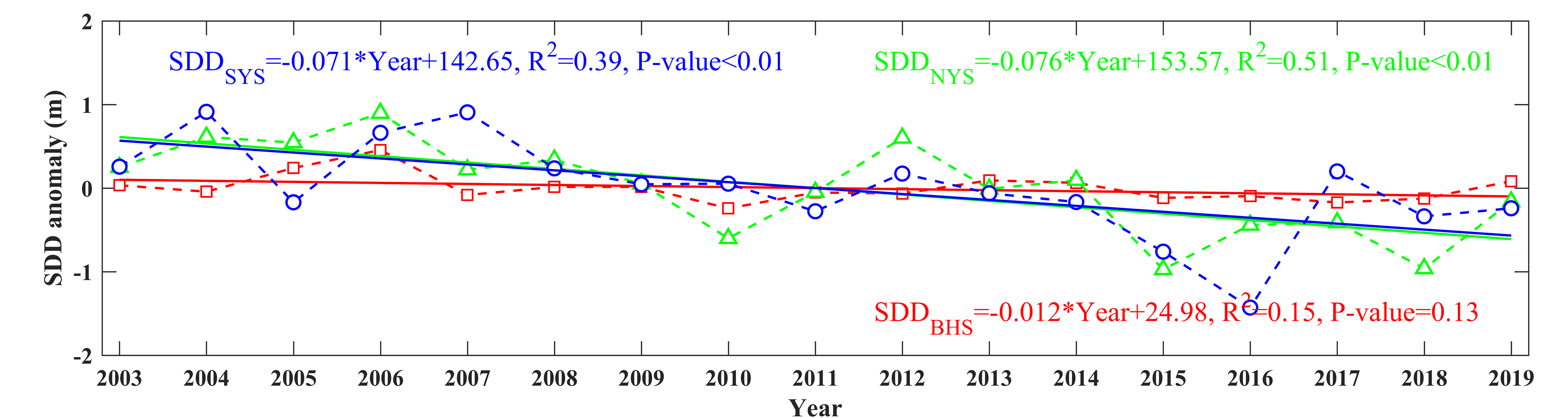
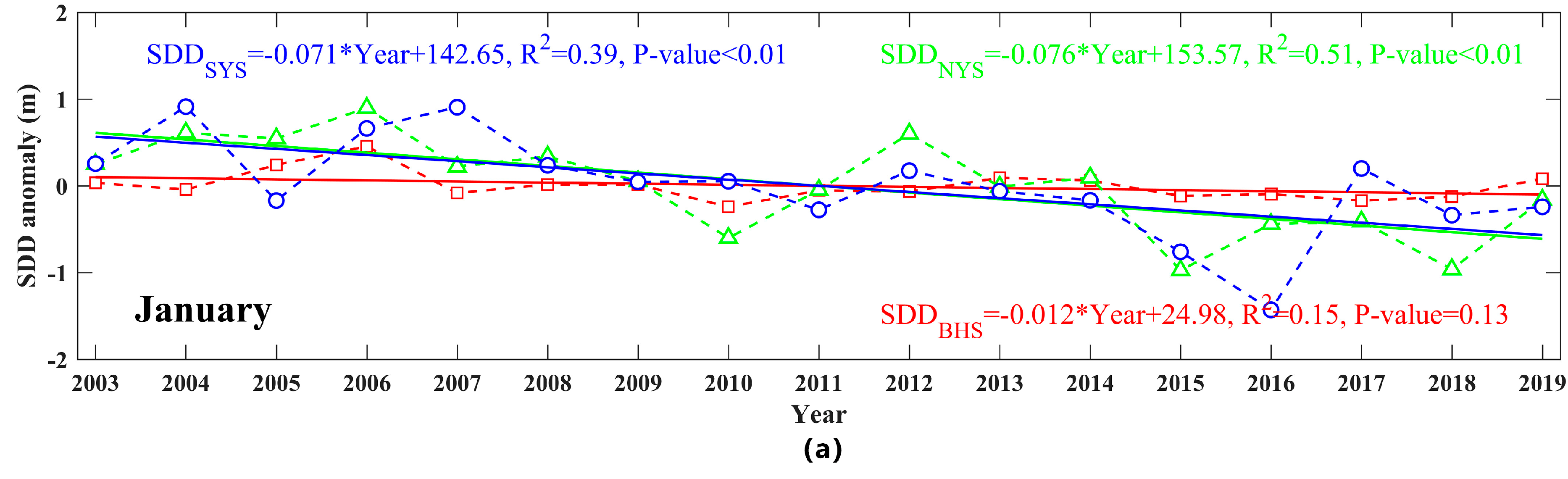
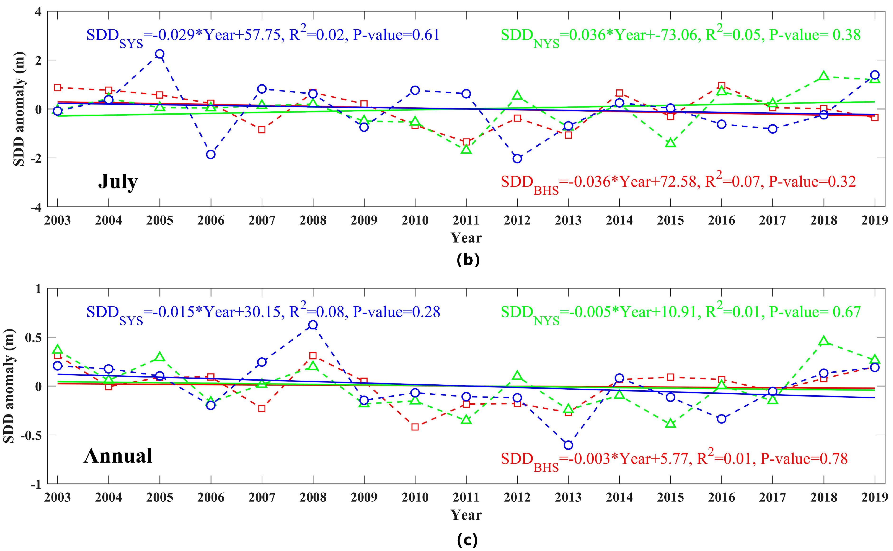
3.1.1. Interannual Variations in SDD Dynamics

For the MODIS L3 monthly mean R_rs images of BYS, the percentage of valid pixels is about 80.4%. The missing data of satellite remote sensing appeared mostly in winter and was mainly caused by cloud cover, contamination of sun glint, atmosphere correction, or adjacency from land. With the confidence in the model description of Lee et al. (2015) in the China seas, monthly mean SDD images of BYS were estimated from MODIS monthly mean R_rs. The spatial distribution of climatological annual mean SDD images from 2003 to 2019 was calculated (Figure 2), and lower/higher-value area is displayed. Overall, it shows a large SDD variation range in the study area (0.4–15.6 m). The lower-value area is found in the Bohai Sea (0.5–4.3 m), and the higher-value area appeared in the center South Yellow Sea, which is consistent with the variation trend of the water depth contour marked in Figure 1. With the influence of the shallow water depth, the terrestrial input by the Yellow River and the Yangtze River, and the coastal currents, the transparency inshore where the water depth is below 50 m is relatively low, and in contrast, the water transparency is high in the deep ocean far from the coastline, which is less affected by the continent. There are tongue-shaped low-transparency areas near Chengshanjiao and southeast of Subei Shoal. The standard deviation of the SDD of the entire sea area is less than 6 m. The lack of data in the northern Jiangsu Shoal and the coastal waters of Hangzhou Bay are largely due to the failure of the atmospheric correction algorithm in the coastal turbid waters.

The MK and SS analysis results for each region in Figure 2 show that the water transparency of most areas of the BYS did not obtain statistical clustering characteristics (1.96 > Z-value > −1.96); insignificant increasing or decreasing trend was observed except for the coastal waters of Haizhou Bay, which showed a significant negative trend (Z-value < −1.96). Although the transparency of the coastal waters in the BHS was also significantly increased, the three bays (Laizhou Bay, Liaodong Bay, and Bohai Bay) have about 3 to 4 months of the ice in winter, which will cause most of the SDD data missing in winter. Therefore, trend analysis is not statistically significant. The SDD in the central BHS has increased, but the time trend is not significant. The NYS area showed an increase in SDD in the northern water depth of less than 50 m, and a negative trend covers the spatial extent of other areas. SDD in the SYS showed an increasing temporal trend in the central part of the YS.

Taking January and July as the representative months of winter and summer, respectively, based on the spatial average of the monthly data of each sea area, linear regression was performed on the data of SDD time anomalies, and the annual average time series were also statistically analyzed (Figure 3). Due to the existence of the winter ice period, the three bays of the BHS were excluded on average and only consider the central region. Regarding the trend of SDD anomalies, the temporal variations of the three sea areas all show a certain degree of fluctuation. In winter, both NYS and SYS areas decreased significantly, and BHS showed an insignificant decrease. In summer, NYS showed an increasing trend, SYS and BHS showed a decrease in variation, but none of the trends were significant. For the insignificant trend, on the one hand, when the new transparency algorithm was established and compared with the measured data, 10% of the uncertainties came from the visual deviation of the in situ measurements; on the other hand, it can be attributed to the use of a unified atmospheric correction algorithm when acquiring MODIS R_rs product data, which leads to a large deviation in the SDD data obtained through inversion. The influence of these uncertain errors was ignored in this study. In terms of annual changes, the SDD of the entire study sea area shows a decreased trend, and the variation rate is lowest in the BHS at 0.003 m y⁻¹ and highest in the SYS at 0.015 m y⁻¹. The trend analysis of the SDD anomaly also shows that before 2009, the water transparency was higher than the annual mean, and lower from 2009 to 2017, which also means that the water quality of the entire sea area may have deteriorated during this period. Since 2017, it shows a weak increasing trend, which implies that the water quality in the study sea area seems to have improved. The variations in water transparency are most likely related to changes in human activities and weather conditions, so more efforts are needed to maintain a healthy marine ecosystem.

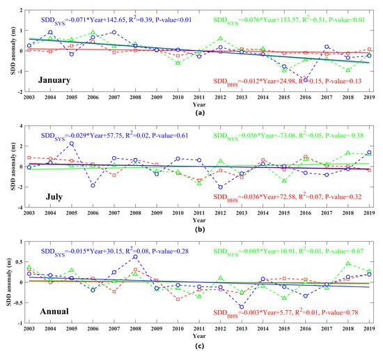
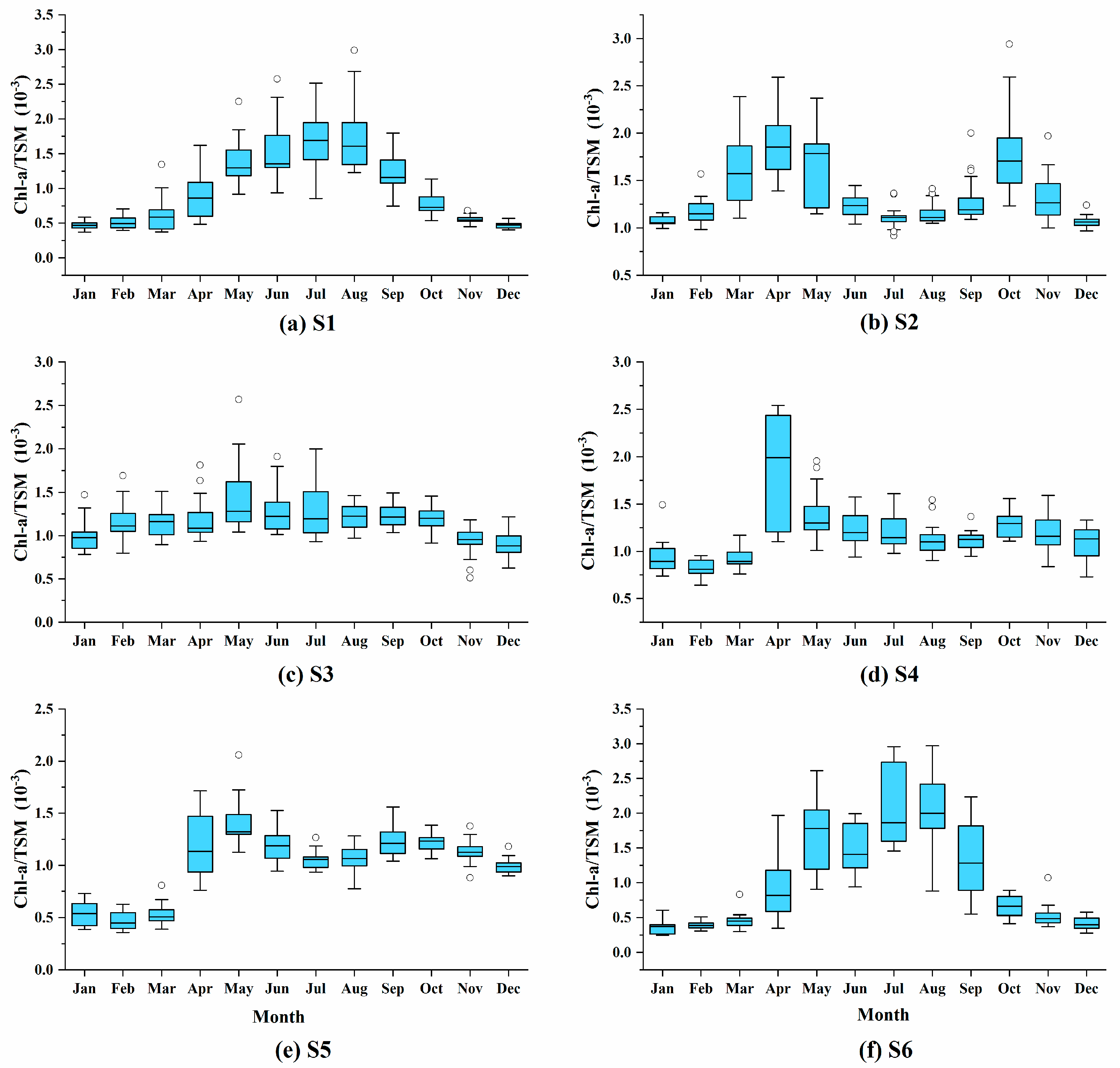
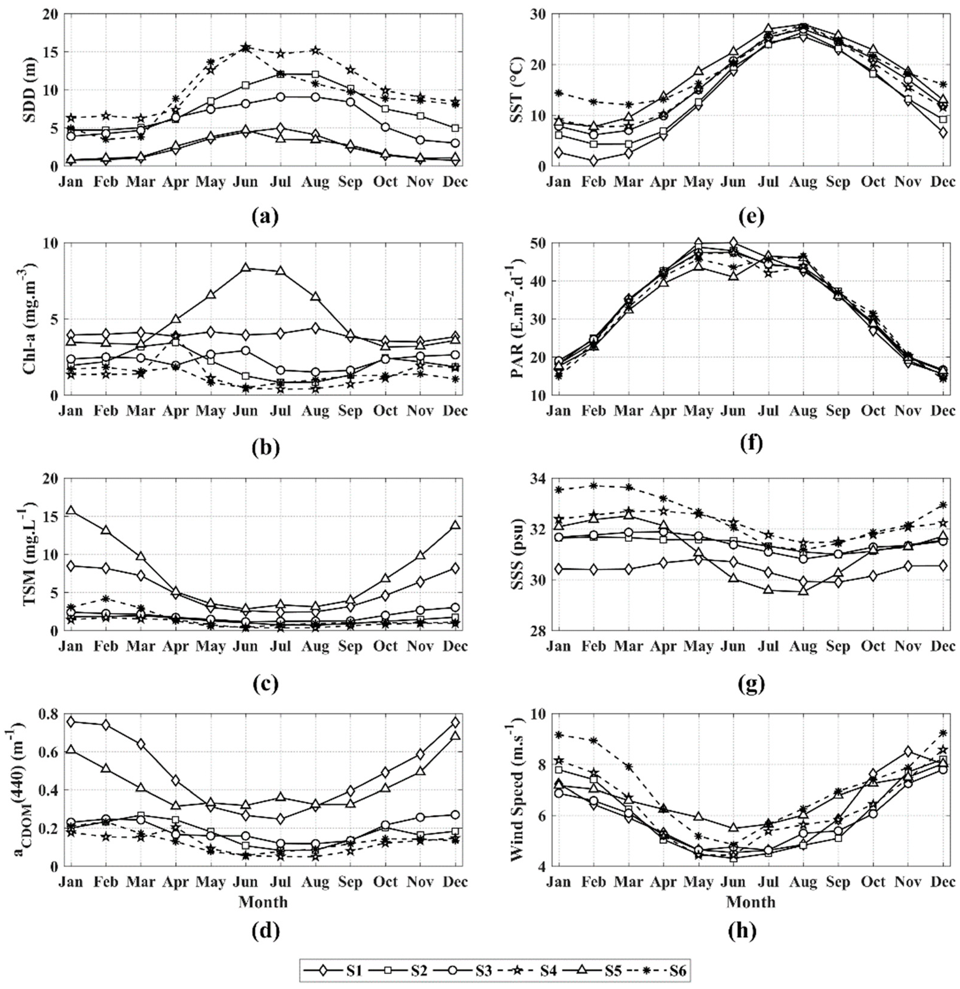
3.1.2. Seasonal Patterns of SDD and Related Marine Environmental Factors

Climatological SDD time series data also indicated seasonal patterns of low in spring and winter and high in summer and autumn, as displayed in Figure 4. Related marine environmental factors, including Chl-a, TSM, CDOM, SST, PAR, SSS, and wind vectors (wind speed and direction) are all given in similar patterns.

In spring, the water transparency is low, less than 4 m in the Bohai Sea, the coastline of the Yellow Sea, Subei Shoal, and Yangtze River estuary. Values are higher in the central South Yellow Sea, reaching 14 m. The low-value area near Chengshanjiao is related to the strong mixing caused by the flow around the peninsula, and also to the sediment of the Yellow River carried by the North Shandong coastal currents. When the SST gradually rises in summer, the increasing thickness of the thermocline strengthens the vertical stability of coastal waters, and the upper and lower layers of seawater are not easily mixed [59], making this the most transparent time of the year. The water transparency is 1.6–8 m in the Bohai Sea and 2.4–19.4 m in the Yellow Sea, which is significantly higher than that in spring. The low-value area in the east of the Subei Shoal decreases to the smallest area of the year. In autumn, as the northwest wind weakens and the northwest wind strengthens, the convective mixing of seawater gradually increases, and the concentration of suspended matter increases, which leads to a general decrease in water transparency. The high-value area in the center of the Bohai Sea no longer exists, and water transparency on the entire sea area is relatively uniform, with its values <5 m. The water transparency range of the Yellow Sea is 0.2–16 m. The water transparency in winter is the lowest among the four seasons. The water transparency in the Bohai Sea is 0.1–2 m, and the spatial difference is the smallest. The transparency of the coastal waters of the Yellow Sea is less than 3 m. Most of the central sea areas in the Yellow Sea are still in high transparency (6–8 m).

From the climatological image of the optical components of the seawater, the regional distribution trends of Chl-a, TSM, and CDOM in the Bohai Sea are relatively consistent: from the high-value area of Bohai Bay, Laizhou Bay, and Liaodong Bay to the low-value area of Bohai Strait. All factors show regular gradient changes, and the isoline is basically consistent with the trend of the coastline. Near the Subei Shoal in the Yellow Sea, coastal currents and terrestrial input leads to the high content of suspended particles and chromophoric dissolved organic matter throughout the whole year. The center of the North Yellow Sea and the South Yellow Sea are mainly affected by the Yellow Sea warm current. The seawater of this area contains a certain portion of suspended sediment and nutrient matter. The Chl-a concentration is relatively high in spring and winter. The coastal waters of the North Yellow Sea and the Shandong Peninsula are affected by the combined action of density currents and coastal currents, and the contours of each factor are almost parallel to the coastline.

As seen from the series of climatological changes of marine environmental factors, the spatial patterns of PAR, SST, and wind vectors are nearly coherent in the seasonal cycles. The PAR is mainly related to solar radiation intensity. Accounting for the difference in solar altitude angles of different seasons, SST presents the characteristics of low in winter and high in summer, and its spatial distribution roughly corresponds to the latitude zone. On account of the East Asian monsoon [60], northerly winds prevail in winter, the average wind speed is about 7–8 m s⁻¹; spring monsoons alternate and wind directions become unstable; in summer, southerly and southeast winds prevail and the average wind speed is about 4–6 m s⁻¹. In terms of the spatial distribution of SSS, the salinity in the near-shore is low, resulting from the input of freshwater from the river, and gradually increases from inshore to offshore. Winter and spring are mainly under the influence of the Yellow Sea warm water mass, and the high-salt water body carried is tongue-shaped, extending to the central Yellow Sea. In summer and autumn, two low-salt areas formed near the mouths of the Yellow River and the Yangtze River are more obvious, and the freshwater input by the rivers extends from the coastal areas to the deep ocean.

3.2. Variations of Marine Environmental Factors and Relevance for SDD

The principal modes obtained by the EOF decomposition can be used to achieve the dominant space and temporal patterns and main impact factors from the time series satellite images [61,62,63]. A strong environmental factor can appear in several principal modes, and there many environmental factors can take effect in one mode. Figure 5 shows spatial patterns (a–c) and temporal amplitudes (d) for the first three SDD EOF modes.

The first SDD mode explains 58.75% of the total variance. The change of spatial patterns is not obviously apparent. The amplitude value is positive everywhere, but the time amplitude changes drastically, indicating that the SDD temporal trends are consistent throughout the study area. The amplitude of the spatial pattern increases from the coast to the open sea, with the largest changes found in the center of the Yellow Sea. It is similar to the annual average SDD image. The corresponding time mode reveals a clear seasonal cycle change signal, which is positive from May to September, indicating that the water transparency is higher than the annual mean, and the other months are negative, indicating that the transparency is lower. It also shows that seasonal ocean and atmospheric processes, such as PAR, SST, and wind vectors, are the important factors that cause periodic changes of the mode. Since the optical components of water also have seasonal cycle changes, they must be included when analyzing the physical processes related to leading patterns. The second and third EOF modes of SDD play a small role in SDD changes. Higher-order EOFs are not considered in this study, and only explain the minor component of the total variance.

The second mode of EOF accounts for 4.14% of the total variance. Combined with the spatial patterns and temporal amplitudes, it decreases in summer and increases in autumn. The transparency changes between the center Yellow Sea and the region near the Yangtze River estuary are opposite. The presence of a thermocline generated by the increase in surface water temperature in the central Yellow Sea in summer prevents the suspended particles at the bottom from mixing with the upper water body. In offshore waters, the shallower water depth and the shallower thermocline weaken the effect of hindering the resuspension of particles. The change of transparency in autumn may be affected by the decrease of freshwater drained down from the Yangtze River estuary and the high-salt water body brought by the Yellow Sea warm water mass. Therefore, this mode is closely related to SST and SSS. The third mode of EOF contains 2.97% of the total variance, and the explained SDD feature is weaker. It shows that the SDD in the central Yellow Sea increases in autumn and winter, whereas the SDD near the coastal area decreases. This may be owing to the increased sea surface wind intensity in autumn and the effect of suspended sediment on the bottom of the coastal waters, which leads to a greater degree of transparency than the central South Yellow Sea. The large spatial amplitude of the southern branch of the Shandong Peninsula and the Bohai Sea is perhaps caused by seasonal blooms from the changes of Chl-a.

Since the overall transparency of the Bohai Sea and the North Yellow Sea are relatively low, the water properties can be regarded to be similar. It should be noted that since the spatial area is relatively small, the characteristics of the signal in this area can be easily covered by the strong signal of the South Yellow Sea when EOF is decomposed. We also performed EOF analysis in the BNYS and SYS areas at the same time. The spatial and temporal modes from the EOF decomposition of long-term data are not shown in this study.

To clarify what environmental factors cause the time changes of SDD in the area of BNYS, SYS, and BYS respectively,

Table 1. Correlation coefficient between SDD EOF temporal modes and marine environmental factors in BNYS, SYS, and BYS.

Region	Temporal Mode	Chl-a	TSM	aCDOM(440)	PAR	SST	SSS	Wind Speed
(Units)		(mg·m−3)	(mg·L−1)	(m−1)	(E·m−2·d−1)	(°C)	(psu)	(m·s−1)
BNYS	PC 1	−0.309	−0.931 *	−0.930 *	0.745 *	0.896 *	−0.356 *	−0.737 *
	PC 2	0.005	0.098	0.163 *	−0.302 *	−0.264 *	0.528 *	0.307 *
	PC 3	−0.283 *	0.078	0.021	−0.219 *	0.005	−0.119	0.138 *
SYS	PC 1	−0.606 *	−0.862 *	−0.875 *	0.702 *	0.838 *	−0.810 *	−0.681 *
	PC 2	0.061	0.150	0.142*	−0.321*	−0.236*	0.235*	0.183
	PC 3	0.139 *	−0.071	−0.053	0.229 *	−0.171	0.186	−0.243 *
BYS	PC 1	−0.508 *	−0.910 *	−0.905 *	0.728 *	0.868 *	−0.778 *	−0.714 *
	PC 2	0.069	0.156 *	0.145 *	−0.276 *	−0.201 *	0.238 *	0.188 *
	PC 3	0.256 *	−0.080	−0.068	0.323 *	−0.244 *	0.304 *	−0.328 *

Note: * p-values < 0.05.

displays the correlation coefficient (r) between SDD EOF temporal modes and the marine environmental factors in each region. The first EOF mode in the BYS shows a strong negative correlation with Chl-a, TSM, a_CDOM(440), SSS, wind speed, and a significant positive correlation with PAR and SST. This mode has the highest correlation with TSM (r = −0.910). Although the weakest correlation with Chl-a (r = −0.508), strong correlation with TSM and CDOM (r = −0.905) illustrates that the change of SDD is determined by the optical components of the water body. The correlation between the second mode and PAR, SST, and SSS is significant, but the correlation is weaker. The third mode has the highest correlation with wind speed, but not strong. It can be taken that PAR, SST, SSS, and wind speed are covariates of SDD changes. It is consistent with the analysis above for each SDD EOF mode on BYS. The contribution rate of PC1 in the BNYS area to the total variance is about 72.64%, which is higher than that of SYS and BYS. The first mode also has a higher correlation with TSM and CDOM, whereas the second and third modes are significantly correlated with SSS and Chl-a, respectively. The correlation between SDD changes and environmental factors in SYS is similar to that of BYS overall, but the first mode has the highest correlation with CDOM.

As the SDD changes in the entire sea area of the BYS have the highest correlation with TSM, and the relationship between the water optical properties and the water components (such as Chl-a concentration and TSM concentration) strongly depends on the composition of suspended particles in water, so it is necessary to characterize the dominant suspended particulate matter types in the water. The ratio of the Chl-a concentration to TSM concentration (Chl-a/TSM) can be considered as a good indicator to quantify the composition of suspended particulates. When the ratio is greater than 0.5 × 10⁻³, it means that the optical properties of the water body are mainly dominated by phytoplankton [64,65,66]. Analyzing the Chl-a/TSM ratio of the six stations (Figure 6), the values are concentrated in the range of 0.25 × 10⁻³–3.0 × 10⁻³, most of which are in the range of 0.5 × 10⁻³–2.5 × 10⁻³. In terms of seasonal changes, S1 and S6 indicate a trend of being high in summer and autumn, and show that the Chl-a/TSM ratio of the sea surface at the S6 station is lower than 0.5 × 10⁻³ in winter and spring, which means the suspended particles are mainly inorganic and mainly resuspended sedimentary particles. Station S1 is strongly mixed in both the upper and lower water column layers, and only shows characteristics of inorganic particles in winter. Other stations show more or less phytoplankton-dominated features throughout the year, which is that the remote sensing reflectance spectrum of the water in these stations shows a higher absorption coefficient in the red band. Stations S2, S4, and S5 showed double peaks in spring and autumn. The water at all stations has a low Chl-a/SPM ratio in spring but a high TSM concentration, which may be carrying more nutrients and more likely to cause algal blooms [67].

Further analysis of the role played by marine environmental factors, SDD changes, and the corresponding seasonal changes of marine environmental factors at the six stations is presented in Figure 7. Overall, the water transparency is the greatest at S4 and S6, and lowest at S1 and S5. The seasonal variation trends of SST, PAR, SSS, and wind speed at each station are roughly the same, but the changes in the optical components of the water body are quite different. The detailed contrastive analysis shows the following features: (1) The SDD changes of S1 and S5 are only different in July; S1 continues to increase whereas S5 decreases. Station S1 is located near the mouth of the Yellow River in the Bohai Sea, and station S5 is near the mouth of the Yangtze River. Comparing the changes in related marine environmental factors from June to August, this trend of change is caused by the optical components of the water at station S5 in July, and can be attributed to the huge amount of freshwater from the Yangtze River estuary. (2) The variation trends of S2 and S3 are similar in spring, but their difference increases afterward. Different from S2, S3 has a higher concentration of Chl-a and CDOM that leads to lower transparency. It may be caused by the large-scale algal blooms that occurred every summer in the western part of the Yellow Sea since 2008, which led to the increase of Chl-a concentration and the decrease of water transparency [68,69]. (3) The water depth at S4 and S6 are greater than 50 m, and the water transparency varies from July to October. Although the TSM at each station is relatively low, S6 is adjacent to the diffusion area of the Yangtze River estuary freshwater. The increase in nutrients in seawater drives the photosynthesis of phytoplankton, and Chl-a increases correspondingly and reduces the water clarity.

4. Discussion

In natural waters, the downward spectral radiation within water bodies decreases with increasing water depth; the attenuation process underwater is closely related to the absorption and scattering of the optical components (water molecules, phytoplankton, total suspended particulate matter, and CDOM) [70,71]. In water dominated by inorganic particulate matter, scattering is relatively more significant to SDD than absorption [1]. In the visible light range, water molecules strongly absorb at red wavelength, whereas scattering is very weak. Phytoplankton has two strong absorption peaks at the blue and red wavelength, and strong scattering at the same time [72]. The total suspended particulate matter is composed of the inorganic part and organic part. Inorganic particulate matter has a high refractive index relative to water molecules, so the light underwater would be strongly scattered, but the optical properties of debris-like organic particulate matter are similar to CDOM [73]. CDOM can absorb the light underwater at the blue band and scatter at the yellow band, thus making the sea surface water present as yellow [74]. The Bohai and the Yellow Seas have typical water characterized as Case II. Apart from water molecules, the three main optical components jointly determine the optical characteristics of the water body. Their absorption and scattering characteristics overlap each other during the underwater light penetration process, and each contribution to SDD is nonlinear [75,76]. The long-term SDD changes in the BYS are highly correlated with TSM and CDOM, indicating that the underwater light attenuation of the entire sea area is mainly due to the combined effect of these two optical components. The fact that chlorophyll-a is not highly correlated with SDD also shows that the contribution of phytoplankton in the study area is masked by other water components. Generally speaking, the influence between phytoplankton and water transparency is reciprocal. On the one hand, the absorption of underwater light by phytoplankton biomass will reduce the amount of light that can penetrate the water body. On the other hand, the reduction of light underwater results in lower carbohydrate content in phytoplankton cells and restricts the growth of phytoplankton [77]. Although the SDD changes in the BYS are mainly caused by TSM and CDOM, there are significant differences in the weights of the three optical components for different types of water [78], and the driving factors for SDD changes are also different [79].

From the perspective of ocean optics and ecology, the effects of marine environmental factors on the changes in water transparency cannot be ignored. As analyzed in Table 1, PAR, SST, SSS, and wind speed are covariates that cause SDD changes in the BYS. These factors directly vary the distribution of underwater light and the process of underwater ecosystems, thereby affecting the primary production of seaweed, microalgae, and benthic organisms [80]. The intensity of PAR, corresponding to the intensity of solar radiation, determines the amount of input that may enter the underwater light field. Due to its regular seasonal changes, it cannot be a decisive variable in the SDD variation. There is also a significant positive correlation between SST and SDD (Figure 7). In summer, the sea surface absorbs more solar radiation, and the sea surface temperature rises. The upper-ocean water body gradually forms a stable thermocline, which prevents upward movements of the bottom particles and nutrients. The material is mixed with the upper water body, so the water transparency is generally higher during this period. At the same time, the increase in water transparency promotes the penetration of solar irradiance, increases the light absorption in the deeper part of the water, and then varies the heat transmission of the upper and middle water bodies of the ocean [81]. Since the global SST has increased year-by-year since 2000 [82,83], it may cause an increase in interannual SDD in the deep-sea area of the Yellow Sea (stations S4 and S6). On the spatial distribution of SSS, low-salinity areas are formed near the coast due to runoff input. A large amount of suspended sediment and CDOM accumulate in the water body, and the CDOM concentration is significantly higher in low-salinity water bodies, but the sediment input is usually trapped there with the high sedimentation rate caused by regional circulation [9,84]. The high-salinity areas in the central Yellow Sea are the mixing of coastal low-salt water bodies with high-salt water bodies carried by the Yellow Sea warm water mass. The significant positive correlation between SDD and SSS (Table 1) further highlights the powerful role of CDOM in light attenuation in water bodies. The wind field is the most important factor that affects the TSM changes, especially in the coastal estuary area. The central Yellow Sea is deeper. The stable thermocline in summer prevents the suspended particles driven by the tide and circulation from reaching the upper water body, and the thermal layer gradually disappeared in autumn, the strong wind intensified the mixing of the upper and lower water bodies, resulting in more bottom sediments suspended.

Furthermore, in the analysis of long-term SDD changes, it is essential to take account of the influences of water depth changes caused by topography and tides [85,86]. As shown in Figure 2, the depth of the coastal waters on the west side of the station S3 and station S5 increases with the distance from the coastline. The SDD changes also show a similar increasing trend, and the contour is approximately parallel to the coastline. For deep-sea areas, especially water areas with fast currents and large tidal height changes, for example, the transparency of seawater at station S6 is lower than that at station S5; it is also considered to be affected by the mixing of tidal currents.

5. Conclusions

In this study, climatological SDD images from 2003 to 2019 are estimated using the innovative mechanistic model of Lee et al. (2015) over MODIS L3 monthly mean R_rs data of BYS. The spatial distribution of annual mean SDD shows lower SDD values (0.5–4.3 m) in the Bohai Sea, but higher values in the center of the South Yellow Sea with a large variation range (0.4–15.6 m). The terrestrial input from the Yellow River and the Yangtze River, and coastal currents, lead to water transparency that is relatively low in the inshore area where the water depth is below 50 m but high in the deep ocean. There are tongue-shaped low-transparency areas near Chengshanjiao and southeast of Subei Shoal. The standard deviation of the SDD of the entire sea area is less than 6 m. The seasonal SDD variations also indicate seasonal patterns of low in spring and winter and high in summer and autumn. On the SDD annual changes analysis of the six stations, water transparency at S1 and S3 both decline and other stations increase.

To determine the main impact factors from the time series satellite images, EOF decomposition was carried out. The dominant space and temporal patterns obtained from EOF analysis show that the first SDD EOF mode in the BYS is the highest, and closely correlated with TSM. The high correlation coefficients of CDOM also illustrate that the SDD variation is mainly dominated by the optical components in the seawater, although correlation with Chl-a is the weakest. The contribution of each optical component to the changes of SDD is found to be different in the seawater with different content of optical components. Meanwhile, the dominant suspended particulate matter composition is characterized by Chl-a/TSM. From the second and third EOF modes, PAR, SST, SSS, and wind speed are found to be the covariates that cause SDD changes in the BYS. Furthermore, the impact of changes in water depth caused by topography and tides also need to be taken into consideration. Future research of SDD changes in the marine ecosystem should consider other influencing factors, such as phytoplankton biomass, algal bloom, and river discharge.

References

- Kirk, J.T.O.; Press, C. Light and photosynthesis in aquatic ecosystems. J. Ecol. 1994, 45. [Google Scholar] [CrossRef]
- Lorenzen, M.W. Use of chlorophyll-Secchi disk relationships. Limnol. Oceanogr. 1980, 25, 371–372. [Google Scholar] [CrossRef]
- Phlips, E.J.; Aldridge, F.J.; Schelske, C.L.; Crisman, T.L. Relationships between light availability, chlorophyll a, and tripton in a large, shallow subtropical lake. Limnol. Oceanogr. 1995, 40, 416–421. [Google Scholar] [CrossRef]
- Kim, S.H.; Yang, C.S.; Ouchi, K. Spatio-Temporal patterns of Secchi depth in the waters around the Korean Peninsula using MODIS data. Estuar. Coast. Shelf Sci. 2015, 164, 172–182. [Google Scholar] [CrossRef]
- Kukushkin, A.S. Long-Term seasonal variability of water transparency in the surface layer of the deep part of the Black Sea. Russ. Meteorol. Hydrol. 2014, 39, 178–186. [Google Scholar] [CrossRef]
- Lathrop, R.G.; Lillesand, T.M.; Yandell, B.S. Testing the utility of simple multi-date Thematic Mapper calibration algorithms for monitoring turbid inland waters. Int. J. Remote Sens. 1991, 12, 2045–2063. [Google Scholar] [CrossRef]
- Kemp, W.M.; Boynton, W.R.; Adolf, J.E.; Boesch, D.F.; Boicourt, W.C.; Brush, G.S.; Cornwell, J.C.; Fisher, T.R.; Glibert, P.M.; Hagy, J.D. Eutrophication of Chesapeake Bay: Historical trends and ecological interactions. Mar. Ecol. Prog. Ser. 2005, 303, 1–29. [Google Scholar] [CrossRef]
- Testa, J.M.; Lyubchich, V.; Zhang, Q. Patterns and trends in Secchi disk depth over three decades in the Chesapeake Bay estuarine complex. Estuaries Coasts 2019, 42, 927–943. [Google Scholar] [CrossRef]
- Taillie, D.M.; O’Neil, J.M.; Dennison, W.C. Water quality gradients and trends in New York Harbor. Reg. Stud. Mar. Sci. 2020, 33. [Google Scholar] [CrossRef]
- Gai, Y.Y.; Yu, D.F.; Zhou, Y.; Yang, L.; Chen, C.; Chen, J. An Improved Model for Chlorophyll-a Concentration Retrieval in Coastal Waters Based on UAV-Borne Hyperspectral Imagery: A Case Study in Qingdao, China. Water 2020, 12, 2769. [Google Scholar] [CrossRef]
- Qiu, Z.; Wu, T.; Su, Y. Retrieval of diffuse attenuation coefficient in the China seas from surface reflectance. Opt. Express 2013, 21, 15287–15297. [Google Scholar] [CrossRef] [PubMed]
- Tyler, J.E. The Secchi disc. Limnol. Oceanogr. 1968, 8, 1–6. [Google Scholar] [CrossRef]
- Preisendorfer, R.W. Secchi disk science: Visual optics of natural waters. Limnol. Oceanogr. 1986, 31, 909–926. [Google Scholar] [CrossRef] [Green Version]
- Fleminglehtinen, V.; Laamanen, M. Long-Term changes in Secchi depth and the role of phytoplankton in explaining light attenuation in the Baltic Sea. Estuar. Coast. Shelf Sci. 2012, 102, 1–10. [Google Scholar] [CrossRef]
- Gregg, W.W. Ocean-Colour Data Merging; IOCCG: Reports of the International Ocean-Colour Coordinating Group, No. 6; International Ocean-Colour Coordinating Group: Monterey, CA, USA, 2007. [Google Scholar]
- Mcclain, C.R. A decade of satellite ocean color observations. Annu. Rev. Mar. Sci. 2009, 1, 19–42. [Google Scholar] [CrossRef] [Green Version]
- Giardino, C.; Bresciani, M.; Villa, P.; Martinelli, A. Application of remote sensing in water resource management: The case study of Lake Trasimeno, Italy. Water Resour. Manag. 2010, 24, 3885–3899. [Google Scholar] [CrossRef]
- Chen, Z.; Mullerkarger, F.E.; Hu, C. Remote sensing of water clarity in Tampa Bay. Remote Sens. Environ. 2007, 109, 249–259. [Google Scholar] [CrossRef]
- Wang, S.L.; Li, J.S.; Zhang, B.; Lee, Z.; Spyrakos, E.; Feng, L.; Liu, C.; Zhao, H.L.; Wu, Y.H.; Zhu, L.P. Changes of water clarity in large lakes and reservoirs across China observed from long-term MODIS. Remote Sens. Environ. 2020, 247. [Google Scholar] [CrossRef]
- Li, N.; Shi, K.; Zhang, Y.L.; Gong, Z.J.; Peng, K.; Zhang, Y.B.; Zha, Y. Decline in transparency of Lake Hongze from long-term MODIS observations: Possible causes and potential significance. Remote Sens. 2019, 11, 177. [Google Scholar] [CrossRef] [Green Version]
- Song, K.S.; Liu, G.; Wang, Q.; Wen, Z.D.; Lyu, L.L.; Du, Y.X.; Sha, L.W.; Fang, C. Quantification of lake clarity in China using Landsat OLI imagery data. Remote Sens. Environ. 2020, 243. [Google Scholar] [CrossRef]
- Liu, D.; Duan, H.T.; Loiselle, S.; Hu, C.M.; Zhang, G.Q.; Li, J.L.; Yang, H.; Thompson, J.R.; Cao, Z.G.; Shen, M.; et al. Observations of water transparency in China’s lakes from space. Int. J. Appl. Earth Obs. Geoinf. 2020, 92, 11. [Google Scholar] [CrossRef]
- Zeng, S.; Lei, S.H.; Li, Y.M.; Lyu, H.; Xu, J.F.; Dong, X.Z.; Wang, R.; Yang, Z.Q.; Li, J.C. Retrieval of Secchi Disk Depth in Turbid Lakes from GOCI Based on a New Semi-Analytical Algorithm. Remote Sens. 2020, 12, 1516. [Google Scholar] [CrossRef]
- Xue, Y.H.; Xiong, X.J.; Liu, Y.Q. Distribution features and seasonal variability of the transparency in offshore waters of China. Adv. Mar. Sci. 2015, 33, 38–44. [Google Scholar] [CrossRef]
- Chen, J.; Han, Q.J.; Chen, Y.L.; Li, Y.D. A Secchi Depth Algorithm Considering the Residual Error in Satellite Remote Sensing Reflectance Data. Remote Sens. 2019, 11, 1948. [Google Scholar] [CrossRef] [Green Version]
- Shang, S.L.; Lee, Z.P.; Shi, L.H.; Lin, G.; Wei, G.M.; Li, X.D. Changes in water clarity of the Bohai Sea: Observations from MODIS. Remote Sens. Environ. 2016, 186, 22–31. [Google Scholar] [CrossRef] [Green Version]
- Mao, Y.; Wang, S.Q.; Qiu, Z.F.; Sun, D.Y.; Bilal, M. Variations of transparency derived from GOCI in the Bohai Sea and the Yellow Sea. Opt. Express 2018, 26, 12191–12209. [Google Scholar] [CrossRef]
- Lee, Z.P.; Shang, S.L.; Hu, C.M.; Du, K.P.; Weidemann, A.; Hou, W.L.; Lin, J.F.; Lin, G. Secchi disk depth: A new theory and mechanistic model for underwater visibility. Remote Sens. Environ. 2015, 169, 139–149. [Google Scholar] [CrossRef] [Green Version]
- Amante, C.; Eakins, B. ETOPO1 1 Arc-minute global relief model: Procedures, data sources and analysis. NOAA technical memorandum NESDIS NGDC-24. Natl. Geophys. Data Cent. NOAA 2009, 10. [Google Scholar] [CrossRef]
- Cui, T.W.; Zhang, J.; Groom, S.; Sun, L.; Smyth, T.; Sathyendranath, S. Validation of MERIS ocean-color products in the Bohai Sea: A case study for turbid coastal waters. Remote Sens. Environ. 2010, 114, 2326–2336. [Google Scholar] [CrossRef]
- Wang, S.Q.; Huan, Y.; Qiu, Z.F.; Sun, D.Y.; Zhang, H.L.; Zheng, L.F.; Xiao, C. Remote sensing of particle cross-sectional area in the Bohai Sea and Yellow Sea: Algorithm development and application implications. Remote Sens. 2016, 8, 841. [Google Scholar] [CrossRef] [Green Version]
- Wei, H.; Shi, J.; Lu, Y.Y.; Peng, Y.A. Interannual and long-term hydrographic changes in the Yellow Sea during 1977–1998. Deep-Sea Res. Part II Top. Stud. Oceanogr. 2010, 57, 1025–1034. [Google Scholar] [CrossRef]
- Jiang, W.; Pohlmann, T.; Sun, J.; Starke, A. SPM transport in the Bohai Sea: Field experiments and numerical modelling. J. Mar. Syst. 2004, 44, 175–188. [Google Scholar] [CrossRef]
- O’Reilly, J.E.; Maritorena, S.; Mitchell, B.G.; Siegel, D.A.; Carder, K.L.; Garver, S.A.; Kahru, M.; McClain, C. Ocean color chlorophyll algorithms for SeaWiFS. J. Geophys. Res. Ocean. 1998, 103, 24937–24953. [Google Scholar] [CrossRef] [Green Version]
- Hu, C.M.; Lee, Z.P.; Franz, B. Chlorophyll aalgorithms for oligotrophic oceans: A novel approach based on three-band reflectance difference. J. Geophys. Res. Ocean. 2012, 117. [Google Scholar] [CrossRef] [Green Version]
- Zhang, M.W.; Tang, J.W.; Dong, Q.; Song, Q.T.; Ding, J. Retrieval of total suspended matter concentration in the Yellow and East China Seas from MODIS imagery. Remote Sens. Environ. 2010, 114, 392–403. [Google Scholar] [CrossRef]
- Frouin, R.; Pinker, R.T. Estimating Photosynthetically Active Radiation (PAR) at the earth’s surface from satellite observations. Remote Sens. Environ. 1995, 51, 98–107. [Google Scholar] [CrossRef]
- Zhu, W.; Yu, Q.; Tian, Y.Q.; Chen, R.F.; Gardner, G.B. Estimation of chromophoric dissolved organic matter in the Mississippi and Atchafalaya river plume regions using above-surface hyperspectral remote sensing. J. Geophys. Res. Ocean. 2011, 116. [Google Scholar] [CrossRef]
- Zhu, W.; Yu, Q. Inversion of chromophoric dissolved organic matter from EO-1 Hyperion imagery for turbid estuarine and coastal waters. IEEE Trans. Geosci. Remote Sens. 2012, 51, 3286–3298. [Google Scholar] [CrossRef]
- Casey, K.S.; Brandon, T.B.; Cornillon, P.; Evans, R. The past, present, and future of the AVHRR Pathfinder SST program. In Oceanography from Space; Springer: Cham, Switzerland, 2010; pp. 273–287. [Google Scholar]
- Saha, K.; Zhao, X.; Zhang, H.; Casey, K.; Zhang, D.; Baker-Yeboah, S.; Kilpatrick, K.; Evans, R.; Ryan, T.; Relph, J. AVHRR Pathfinder Version 5.3 Level 3 Collated (L3C) Global 4 km Sea Surface Temperature for 1981–Present; NOAA National Centers for Environmental Information: Asheville, NC, USA, 2018. [Google Scholar] [CrossRef]
- Bentamy, A.; Grodsky, S.A.; Carton, J.A.; Croizé-Fillon, D.; Chapron, B. Matching ASCAT and QuikSCAT winds. J. Geophys. Res. Ocean. 2012, 117. [Google Scholar] [CrossRef] [Green Version]
- Mortin, J.; Howell, S.E.L.; Wang, L.; Derksen, C.; Svensson, G.; Graversen, R.G.; Schrøder, T.M. Extending the QuikSCAT record of seasonal melt-freeze transitions over Arctic sea ice using ASCAT. Remote Sens. Environ. 2014, 141, 214–230. [Google Scholar] [CrossRef]
- Salon, S.; Cossarini, G.; Bolzon, G.; Feudale, L.; Lazzari, P.; Teruzzi, A.; Solidoro, C.; Crise, A. Marine Ecosystem forecasts: Skill performance of the CMEMS Mediterranean Sea model system. Ocean Sci. Discuss. 2019. [Google Scholar] [CrossRef]
- Nardelli, B.B. A novel approach for the high-resolution interpolation of in situ sea surface salinity. J. Atmos. Ocean. Technol. 2012, 29, 867–879. [Google Scholar] [CrossRef]
- Doron, M.; Babin, M.; Hembise, O.; Mangin, A.; Garnesson, P. Ocean transparency from space: Validation of algorithms using MERIS, MODIS and SeaWiFS data. Remote Sens. Environ. 2011, 115, 2986–3001. [Google Scholar] [CrossRef]
- Shi, K.; Zhang, Y.L.; Song, K.S.; Liu, M.L.; Zhou, Y.Q.; Zhang, Y.B.; Li, Y.; Zhu, G.W.; Qin, B.Q. A semi-analytical approach for remote sensing of trophic state in inland waters: Bio-Optical mechanism and application. Remote Sens. Environ. 2019, 232, 12. [Google Scholar] [CrossRef]
- Lee, Z.P. A model for the diffuse attenuation coefficient of downwelling irradiance. J. Geophys. Res. Ocean. 2005, 110. [Google Scholar] [CrossRef]
- Lee, Z.P.; Hu, C.M.; Shang, S.L.; Du, K.P.; Lewis, M.; Arnone, R.; Brewin, R. Penetration of UV-visible solar radiation in the global oceans: Insights from ocean color remote sensing: Penetration of UV-visible solar light. J. Geophys. Res. Ocean. 2013, 118, 4241–4255. [Google Scholar] [CrossRef] [Green Version]
- Pope, R.M.; Fry, E.S. Absorption spectrum (380–700 nm) of pure water. II. Integrating cavity measurements. Appl. Opt. 1997, 36, 8710–8723. [Google Scholar] [CrossRef]
- Smith, R.C.; Baker, K.S. Optical properties of the clearest natural waters (200–800 nm). Appl. Opt. 1981, 20, 177–184. [Google Scholar] [CrossRef]
- Blackwell, H.R. Contrast thresholds of the human eye. JOSA 1946, 36, 624–643. [Google Scholar] [CrossRef]
- Fuentes, I.; van Ogtrop, F.; Vervoort, R.W. Long-Term surface water trends and relationship with open water evaporation losses in the Namoi catchment, Australia. J. Hydrol. 2020, 584. [Google Scholar] [CrossRef]
- Gocic, M.; Trajkovic, S. Analysis of changes in meteorological variables using Mann-Kendall and Sen’s slope estimator statistical tests in Serbia. Glob. Planet. Chang. 2013, 100, 172–182. [Google Scholar] [CrossRef]
- Bradley, B.A.; Jacob, R.W.; Hermance, J.F.; Mustard, J.F. A curve fitting procedure to derive inter-annual phenologies from time series of noisy satellite NDVI data. Remote Sens. Environ. 2007, 106, 137–145. [Google Scholar] [CrossRef]
- North, G.R. Empirical orthogonal functions and normal modes. J. Atmos. Sci. 1984, 41, 879–887. [Google Scholar] [CrossRef] [Green Version]
- Preisendorfer, R.W.; Mobley, C.D. Principal component analysis in meteorology and oceanography. Dev. Atmos. Sci. 1988, 17. [Google Scholar] [CrossRef]
- North, G.R.; Bell, T.L.; Cahalan, R.F.; Moeng, F.J. Sampling errors in the estimation of empirical orthogonal functions. Mon. Weather Rev. 1982, 110, 699–706. [Google Scholar] [CrossRef]
- Zhu, L.B.; Zhao, B.R. Distributions and variations of the transparency in the Bohai Sea, Yellow Sea and East China Sea. Trans. Oceanol. Limnol. 1991, 1–11. [Google Scholar] [CrossRef]
- Su, J. Circulation dynamics of the China Seas north of 18° N. Sea 1998, 11, 483–505. [Google Scholar] [CrossRef]
- Tew-Kai, E.; Marsac, F. Patterns of variability of sea surface chlorophyll in the Mozambique Channel: A quantitative approach. J. Mar. Syst. 2009, 77, 77–88. [Google Scholar] [CrossRef]
- Shi, W.; Wang, M.H. Satellite views of the Bohai Sea, Yellow Sea, and East China Sea. Prog. Oceanogr. 2012, 104, 30–45. [Google Scholar] [CrossRef]
- Rinaldi, E.; Nardelli, B.B.; Volpe, G.; Santoleri, R. Chlorophyll distribution and variability in the Sicily Channel (Mediterranean Sea) as seen by remote sensing data. Cont. Shelf Res. 2014, 77, 61–68. [Google Scholar] [CrossRef]
- Sun, D.Y.; Li, Y.M.; Wang, Q.; Le, C.F.; Lv, H.; Huang, C.C.; Gong, S.Q. Specific inherent optical quantities of complex turbid inland waters, from the perspective of water classification. Photochem. Photobiol. Sci. 2012, 11, 1299–1312. [Google Scholar] [CrossRef] [PubMed]
- Sun, D.; Li, Y.; Le, C.; Shi, K.; Huang, C.; Gong, S.; Yin, B. A semi-analytical approach for detecting suspended particulate composition in complex turbid inland waters (China). Remote Sens. Environ. 2013, 134, 92–99. [Google Scholar] [CrossRef]
- Xue, K.; Ma, R.H.; Shen, M.; Li, Y.; Duan, H.T.; Cao, Z.G.; Wang, D.; Xiong, J.F. Variations of suspended particulate concentration and composition in Chinese lakes observed from Sentinel-3A OLCI images. Sci. Total Environ. 2020, 721. [Google Scholar] [CrossRef] [PubMed]
- Binding, C.E.; Greenberg, T.A.; Bukata, R.P. An analysis of MODIS-derived algal and mineral turbidity in Lake Erie. J. Gt. Lakes Res. 2012, 38, 107–116. [Google Scholar] [CrossRef]
- Al Kaabi, M.R.; Zhao, J.; Ghedira, H. MODIS-Based Mapping of Secchi Disk Depth Using a Qualitative Algorithm in the Shallow Arabian Gulf. Remote Sens. 2016, 8, 423. [Google Scholar] [CrossRef] [Green Version]
- Li, L.; Xing, Q.G.; Li, X.R.; Yu, D.F.; Zhang, J.; Zou, J.Q. Assessment of the Impacts from the World’s Largest Floating Macroalgae Blooms on the Water Clarity at the West Yellow Sea Using MODIS Data (2002–2016). IEEE J. Sel. Top. Appl. Earth Obs. Remote Sens. 2018, 11, 1397–1402. [Google Scholar] [CrossRef]
- Padial, A.A.; Thomaz, S.M. Prediction of the light attenuation coefficient through the Secchi disk depth: Empirical modeling in two large Neotropical ecosystems. Limnology 2008, 9, 143–151. [Google Scholar] [CrossRef]
- Lee, Z.P.; Shang, S.L.; Qi, L.; Yan, J.; Lin, G. A semi-analytical scheme to estimate Secchi-disk depth from Landsat-8 measurements. Remote Sens. Environ. 2016, 177, 101–106. [Google Scholar] [CrossRef]
- Chaves, J.E.; Werdell, P.J.; Proctor, C.W.; Neeley, A.R.; Freeman, S.A.; Thomas, C.S.; Hooker, S.B. Assessment of ocean color data records from MODIS-Aqua in the western Arctic Ocean. Deep Sea Res. Part II Top. Stud. Oceanogr. 2015, 118, 32–43. [Google Scholar] [CrossRef]
- Uudeberg, K.; Aavaste, A.; Koks, K.L.; Ansper, A.; Uusoue, M.; Kangro, K.; Ansko, I.; Ligi, M.; Toming, K.; Reinart, A. Optical water type guided approach to estimate optical water quality parameters. Remote Sens. 2020, 12, 391. [Google Scholar] [CrossRef] [Green Version]
- Belanger, S.; Babin, M.; Larouche, P. An empirical ocean color algorithm for estimating the contribution of chromophoric dissolved organic matter to total light absorption in optically complex waters. J. Geophys. Res. Ocean. 2008, 113, 14. [Google Scholar] [CrossRef] [Green Version]
- Alikas, K.; Kratzer, S. Improved retrieval of Secchi depth for optically-complex waters using remote sensing data. Ecol. Indic. 2017, 77, 218–227. [Google Scholar] [CrossRef]
- Sun, D.Y.; Ling, Z.B.; Wang, S.Q.; Qiu, Z.F.; Huan, Y.; Mao, Z.H.; He, Y.J. A remote-sensing method to estimate bulk refractive index of suspended particles from GOCI satellite measurements over Bohai Sea and Yellow Sea. Appl. Sci. 2020, 10, 23. [Google Scholar] [CrossRef] [Green Version]
- Leach, T.H.; Beisner, B.E.; Carey, C.C.; Pernica, P.; Rose, K.C.; Huot, Y.; Brentrup, J.A.; Domaizon, I.; Grossart, H.; Ibelings, B.W. Patterns and drivers of deep chlorophyll maxima structure in 100 lakes: The relative importance of light and thermal stratification. Limnol. Oceanogr. 2018, 63, 628–646. [Google Scholar] [CrossRef] [Green Version]
- Feng, L.; Hou, X.J.; Zheng, Y. Monitoring and understanding the water transparency changes of fifty large lakes on the Yangtze Plain based on long-term MODIS observations. Remote Sens. Environ. 2019, 221, 675–686. [Google Scholar] [CrossRef]
- Capuzzo, E.; Stephens, D.; Silva, T.H.; Barry, J.; Forster, R.M. Decrease in water clarity of the southern and central North Sea during the 20th century. Glob. Chang. Biol. 2015, 21, 2206–2214. [Google Scholar] [CrossRef] [Green Version]
- Gattuso, J.; Gentili, B.; Duarte, C.M.; Kleypas, J.A.; Middelburg, J.J.; Antoine, D. Light availability in the coastal ocean: Impact on the distribution of benthic photosynthetic organisms and their contribution to primary production. Biogeosciences 2006, 3, 489–513. [Google Scholar] [CrossRef] [Green Version]
- Lewis, M.R.; Kuring, N.; Yentsch, C.S. Global patterns of ocean transparency: Implications for the new production of the open ocean. J. Geophys. Res. 1988, 93, 6847–6856. [Google Scholar] [CrossRef]
- Guemas, V.; Doblasreyes, F.J.; Andreuburillo, I.; Asif, M. Retrospective prediction of the global warming slowdown in the past decade. Nat. Clim. Chang. 2013, 3, 649–653. [Google Scholar] [CrossRef]
- He, X.Q.; Pan, D.L.; Bai, Y.; Wang, T.Y.; Chen, C.T.A.; Zhu, Q.K.; Hao, Z.Z.; Gong, F. Recent changes of global ocean transparency observed by SeaWiFS. Cont. Shelf Res. 2017, 143, 159–166. [Google Scholar] [CrossRef]
- Palinkas, C.M.; Halka, J.P.; Li, M.; Sanford, L.P.; Cheng, P. Sediment deposition from tropical storms in the upper Chesapeake Bay: Field observations and model simulations. Cont. Shelf Res. 2014, 86, 6–16. [Google Scholar] [CrossRef]
- Aksnes, D.L.; Ohman, M.D.; Riviere, P. Optical effect on the nitracline in a coastal upwelling area. Limnol. Oceanogr. 2007, 52, 1179–1187. [Google Scholar] [CrossRef]
- Dupont, N.; Aksnes, D.L. Centennial changes in water clarity of the Baltic Sea and the North Sea. Estuar. Coast. Shelf Sci. 2013, 131, 282–289. [Google Scholar] [CrossRef] [Green Version]