Article

Evaluation of Pre-Earthquake Anomalies of Borehole Strain Network by Using Receiver Operating Characteristic Curve

1
Key Laboratory of Geo-Exploration Instrumentation, Ministry of Education, Jilin University, Changchun 130061, China
2
The College of Instrumentation and Electrical Engineering, Jilin University, Changchun 130061, China
3
Graduate School of Science, Chiba University, Inage, Chiba 263-8522, Japan
4
Center for Environmental Remote Sensing, Chiba University, Inage, Chiba 263-8522, Japan
5
Istituto Nazionale di Geofisica e Vulcanologia, Via di Vigna Murata, 605, 00143 Rome, Italy
6
School of Information Science and Technology, Hainan Normal University, Haikou 571158, China
*
Author to whom correspondence should be addressed.
Submission received: 2 December 2020 / Revised: 24 January 2021 / Accepted: 29 January 2021 / Published: 1 February 2021

Abstract

:
In order to monitor temporal and spatial crustal activities associated with earthquakes, ground- and satellite-based monitoring systems have been installed in China since the 1990s. In recent years, the correlation between monitoring strain anomalies and local major earthquakes has been verified. In this study, we further evaluate the possibility of strain anomalies containing earthquake precursors by using Receiver Operating Characteristic (ROC) prediction. First, strain network anomalies were extracted in the borehole strain data recorded in Western China during 2010–2017. Then, we proposed a new prediction strategy characterized by the number of network anomalies in an anomaly window, N a n o , and the length of alarm window, T a l m . We assumed that clusters of network anomalies indicate a probability increase of an impending earthquake, and consequently, the alarm window would be the duration during which a possible earthquake would occur. The Area Under the ROC Curve (AUC) between true predicted rate, t p r , and false alarm rate, f p r , is measured to evaluate the efficiency of the prediction strategies. We found that the optimal strategy of short-term forecasts was established by setting the number of anomalies greater than 7 within 14 days and the alarm window at one day. The results further show the prediction strategy performs significantly better when there are frequent enhanced network anomalies prior to the larger earthquakes surrounding the strain network region. The ROC detection indicates that strain data possibly contain the precursory information associated with major earthquakes and highlights the potential for short-term earthquake forecasting.

Graphical Abstract

1. Introduction

It has been observed that the preparatory process and the occurrence of shallow earthquakes are usually accompanied by crustal deformation. Precise observations of surface displacement, using data from GNSS satellites, strainmeters and seismographs all over the world, allow the investigation of complex tectonic structures [1,2,3] and the prediction of short- and medium-term earthquakes [4,5]. However, earthquakes have complicated changing spatio-temporal distribution characteristics, which makes the evaluation of earthquake-related deformation data highly challenging. In recent years, various studies have attempted to understand the interactions and relationships between strain data and earthquakes [6,7,8,9], including those related to the 2008 Wenchuan earthquake in China [10,11] and the 2011 Tohoku earthquake in Japan [12,13,14]. Deformation data represented by borehole strain measurements are also considered to contribute to the estimation of crustal changes. These measurements also play an important role in analysing geodynamic processes, such as those related to volcanic activity [15], slow earthquakes [16,17], and moreover precursory activity [6,18,19,20].
Although borehole strain have been considered to record some pre-earthquake anomalies [8,9,21], whether these anomalies contain precursory information and their use in forecasting of major earthquakes were not evaluated. Receiver Operating Characteristic (ROC) analysis has previously been employed for short-term forecasting to explore whether earthquake precursor information can be obtained from geophysical observations of precursor anomalies [22,23]. Prediction strategies are based on an alarm model that detects and classifies the extracted anomalies extracted and targets earthquake events, thereby evaluating whether measurements contain precursory information for large earthquakes. Recently, various geophysical measurements have indicated the potential for earthquake forecasting [24,25,26], through GPS data [27] and electromagnetic measurements [28,29,30,31]. However, current alarm models only focus on a single anomaly and underestimate the clustering of earthquake anomalies [32,33], which may increase the risk of inaccurate results from short-term forecasting.
In this study, we employ complex networks to jointly investigate borehole strain observations from multiple stations, using seven YRY-4 borehole strainmeter measurements in Western China from 2010 to 2017. We then propose a new prediction strategy to test enhanced networks clustering and earthquake occurrences using ROC analysis and assess its significance related to earthquakes. Furthermore, we discuss the efficiency of the strategy under the influence of different factors. Also, by comparing with GNSS geodetic data, we found that the prediction strategy performs more significantly when there are frequent enhanced network anomalies prior to the earthquakes.

2. Data and Observations

2.1. Borehole Strain Observations

More than 40 YRY-4 borehole strainmeters have been installed in China with the aim of coordinating with satellite-based measurement systems and monitoring surface deformation associated with earthquakes. Surrounding the north and south sides of active fault zones, such as the Longmenshan fault zone and Haiyuan fault zone, we selected the following monitoring sights: YC, HY, LX, GZ, ZT, YS, and TC, all of which yield fairly good data with long-term continuity. Table 1 lists the detailed information of the seven stations, and Figure 1 shows their locations and the regional tectonic settings.
YRY-4 borehole strainmeters sample every minute with a resolution of nearly one-billionth strain changes. The strainmeters can test the quality and reliability of the observations through a self-consistency function, because of their four gauges arranged at 45 intervals. Consequently, the arrangement produces four components [21]. In this study, the strain data were collected from 1 January 2010 to 10 August 2017, and we applied the areal strain, S a , which is transformed by half of the sum of the four observed components and describes the subsurface strain state [21].

2.2. Studied Earthquakes

In this study, we employed the E s parameter, which considers the magnitude of the earthquake and the epicentral distance to identify earthquake events. The E s index is the daily sum of the local earthquake energy, whereas E s is the local energy of an earthquake in the borehole strain network defined by the following equation and the local energy of a single station is shown by the multiplier in the root sign [28,34]:
E s = 1 d a y E s
E s = i = 1 M 10 4.8 + 1.5 m r i 2 M
Here, m and r i are the magnitude of the earthquake and the epicentral distance of each site, respectively, and M is the number of sites. We selected the earthquakes in the area 24 39 N, 98 106 E during 1 January 2010 to 10 August 2017. It should be noted that all the events occurred within the study area during the study period are shallow earthquakes (less than 60 km, mostly less than 30 km), and the earthquakes with magnitude greater than 1.0 were taken into account. To avoid repeated detection of the same process, we have declustered the earthquake catalog by the traditional Reasenberg declustering algorithm, obtained from the Zmap toolbox [35,36]. The completeness of the declustering earthquake catalog is around 1.5, and there are 162 earthquakes of M s 4.0 , 30 earthquakes of M s 5.0 , 9 earthquakes of M s 5.7 and 2 earthquakes of M s 7.0 . The local seismicity and the daily E s are shown in Figure 2. First, we considered that an earthquake occurred if the E s index on a given day exceeded 10 7 J/km 2 . There are 26 target earthquakes, and their detailed information is presented in Table 2. If 10 7 is converted to magnitude, when the average epicentral distance in the network is about 440 km, generally an earthquake should be greater than Ms5.0. We only listed the type of fault of an earthquake when the seismic moment tensors are available.

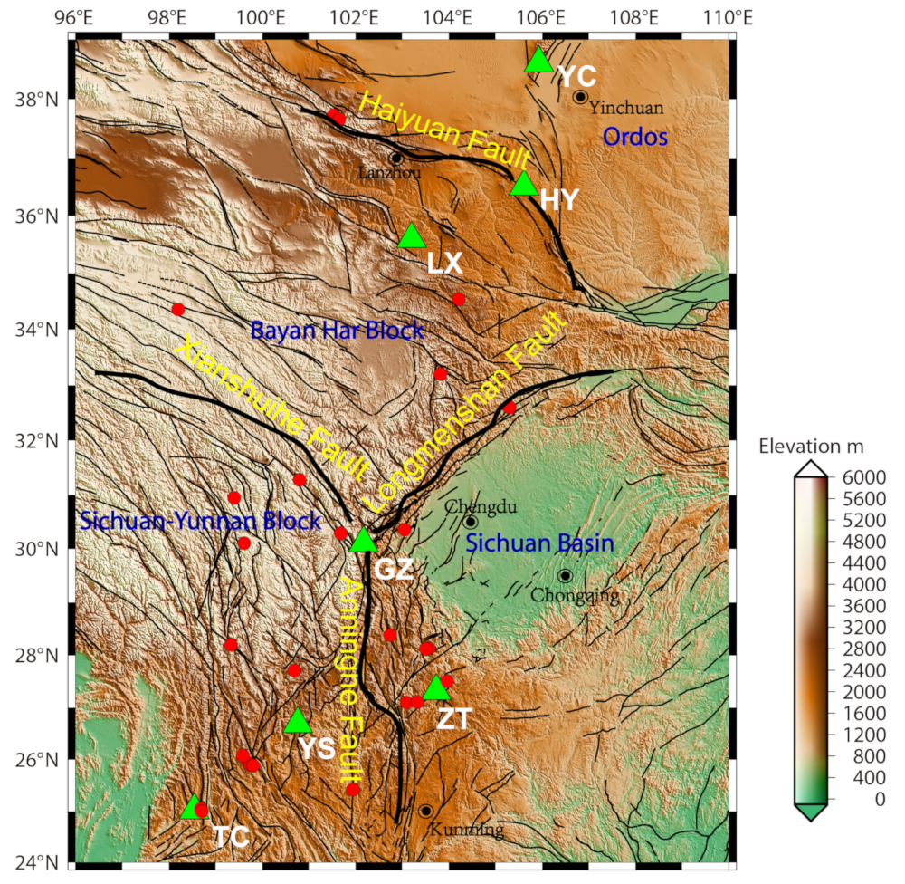
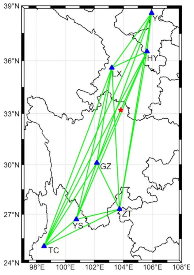
2.3. Tectonic Settings in Brief

The Longmenshan, the Xianshuihe and the Anninghe fault reflect the structural characteristics of the compression of the Yangtze block by the Qinghai Tibet Plateau, as shown in Figure 1. After a long period of geological development, these three fault zones have become the primary zonal faults of Bayan Har Block, Sichuan Basin and Sichuan-Yunnan Block. The total regional stress in this area comes from the compression of the Qinghai Tibet Plateau in the northwest direction [37]. However, the fault structure in this area is diversified, because of the complex geological environments. The Longmenshan fault, which shows a thrust motion from south to north, can be divided into three main faults: the Maoxian-Wenchuan fault (southern segment), the Beichuan-Yingxiu fault (central segment) and the Anxian-Guanxian fault (northern segment) [38]. These three faults are imbricate and all dip northwestward. At the depth of 20–24 km, they converge and merge into a gently inclined reverse fault, which becomes the dominant structure of the Qinghai Tibet Plateau napping over the Sichuan Basin [39,40]. The southernmost end of Xianshuihe fault is the approximately north-south striking Anninghe fault, also known as the Xianshuihe-Anninghe fault zone; it is a large left-lateral strike-slip shear zone [39,41]. The Haiyuan fault is an important active fault zone in the northeastern border of the Qinghai Tibet Plateau, which separates the Bayan Har Block of Qinghai Tibet Plateau from the relatively stable Ordos plate. Its present movement mode is mainly left-lateral strike-slip with thrust component [42].

3. Data Analysis

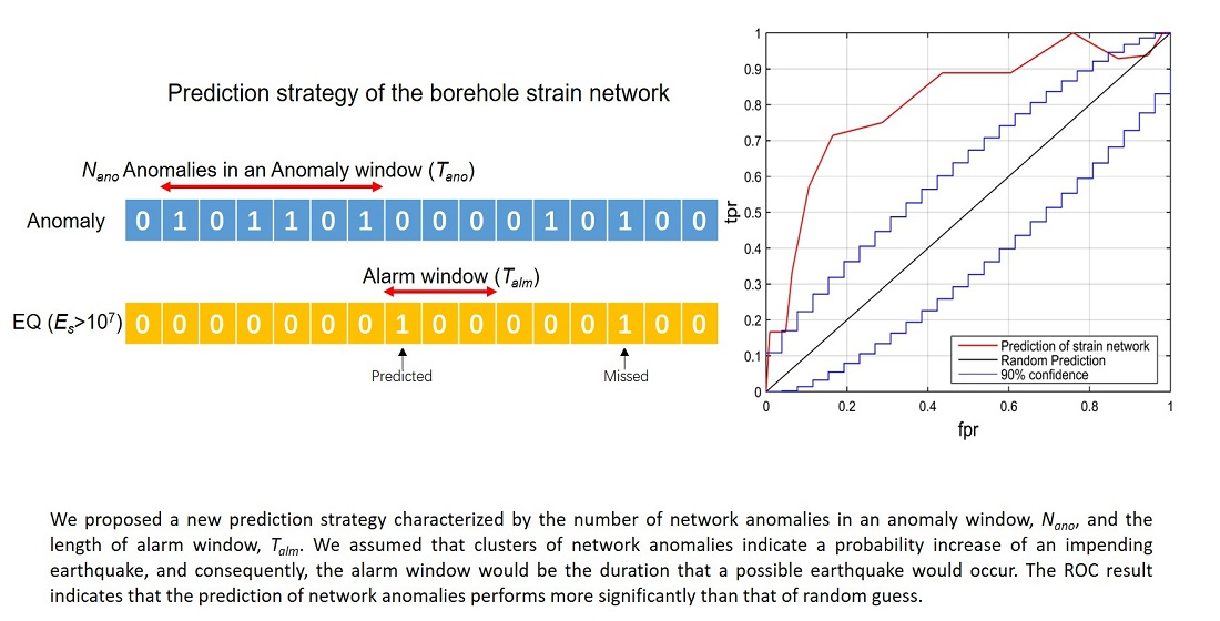
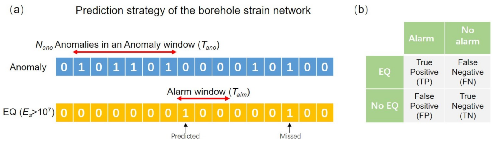
3.1. Extracting Network Anomalies of Borehole Strain

Complex networks can be used as an abstraction of strain monitoring systems to express concealed interactions or relationships between spatial and temporal characteristics [43,44,45,46,47,48,49]. we defined a borehole strain network by a graph consisting of M nodes and a set of edges between nodes. M nodes are on behalf of M borehole stations, while edges are defined by significant relationship between two nodes [50]. An adjacency matrix is applied to describe the graph; A = a i j , i , j V . The correlation between the sequences of length n from two nodes, P = P i and Q = Q j , i , j V , is defined as
R P Q = t = 1 n ( p t p ¯ ) ( q t q ¯ ) t = 1 n ( p t p ¯ ) 2 t = 1 n ( q t q ¯ ) 2 .
Here, p ¯ and q ¯ are the means of P and Q, respectively, and P and Q are the strain components of each observation site [50]. The adjacency matrix A = a i j , i , j V acquires the components that were assigned as “one” if the absolute value of R P Q was greater than 0.8, and as “zero” if R P Q was less than 0.8, indicating whether nodes i and j were connected or not connected. To monitor the changes in the borehole strain network connection, the network degree is used based on the adjacency matrix A . The degree k i of a node is defined as the total number of edges connected to that node in a borehole strain network:
k i = j = 1 M a i j .
Then, the network degree is calculated as the mean value of the k i , ( i = 1 , , M ) in the network, which is expressed as follows:
k ¯ = 1 M i = 1 M k i .
The greater the network degree, the stronger the connection between networks; otherwise, the nodes are considered to be weakly connected, indicating a disordered network. Figure 3 shows an example of the strain network result of 2017 Ms7.0 Jiuzhaigou earthquake, Sichuan. The green lines represent the connections between two stations. It is a fully connected network of that day. The red star shows the epicenter of the earthquake. The daily network degree together with the seismicity and the daily Es are shown in Figure 2 for the complete period of 2010–2017.

3.2. Evaluation of Strain Network Anomalies and Earthquake Occurrence

Due to an increase in the spatiotemporal coherence during earthquake precursory activity [31,50,51], we assumed that the network would be highly connected during such activities. In order to explore the correlations between strain network connection and earthquakes, we proposed a prediction model to test their relationship through a Receiver Operating Characteristic (ROC) curve. The prediction strategy is shown in Figure 4. We analysed how many anomalies of the strain network degree, N a n o , are in an anomaly window, T a n o , where the first day and last day of an anomaly window are required to be anomalous. An alarm window, T a l m , is described as the period in which an impending earthquake would occur. First, we select a threshold to define the anomalies in the strain network degrees. An anomaly is detected when the network degree exceeds the threshold. Next, if the anomalies ( N a n o ) in the alarm window ( T a n o ) account for more than half (as shown in Figure 4, the length of the anomaly window is 6 and the number of anomalies exceeds 3), we assume that a target earthquake with E s 10 7 will occur in the following alarm window, T a l m .
A target earthquake is labelled as predicted if it falls in the alarm window, or as missed if it falls outside the window. The selected threshold is set to vary from the maximum to the minimum network degree. Consequently, the number of anomalies changes from 0 to the length of the sequence. As a result, t p r and f p r change from 0.0 to 1.0. Thus, the confusion matrix shown in Figure 4b can be used to estimate the true positive rates, t p r , and false positive rates, f p r . We set t p r = T P / ( T P + F N ) and f p r = F P / ( F P + T N ) [31,52]. Figure 5 shows an ROC detection result with t p r against f p r . For a given alarm rate, t p r , the probability of n 1 predictions in n target earthquakes is subject to a binomial distribution [28]:
B ( n 1 | n , t p r ) = C n n 1 ( t p r ) n 1 ( 1 t p r ) ( n n 1 ) .
As a result, the diagonal line in the ROC diagram indicates a prediction by random guessing [24,53,54], and the confidence interval of the true positive rate at each alarm rate can be computed. Any prediction above the diagonal line shows that the number of predicted earthquakes is better than that of false alarm days. Next, the Area Under the Curve (AUC) is introduced to evaluate the efficiency of the prediction. The expected area of random prediction is 0.5, where an area greater than 0.5 indicates that the strain network anomalies may contain precursory earthquake information. The result in Figure 5 shows that the prediction for N a n o = 7 and T a l m = 1 days is obviously better than random guess with AUC = 0.81.

4. Results

To reduce the contingency of ROC detection, we performed statistical studies based on Superposed Epoch Analysis (SEA) of the strain network during 2010–2017 preferentially. SEA is a statistical method to highlight typical features of a special event by reducing random noise by superposition [55,56,57]. First, if there is a network anomaly, we count one for that corresponding day for the whole dataset. Here, we set the threshold of the network degree to 4. Then, for each target earthquake, we extracted a data set of 45 days before and 30 days after its occurrence day. We repeated this procedure for the 26 target earthquakes, and then superposed the counts for all data sets. We performed the SEA results of 1-day count and 5-day counts as shown in Figure 6, respectively. To evaluate statistical significance, we randomly selected 26 days instead of studied earthquakes in the whole dataset, and conducted the same procedure. We repeated such random SEA tests 10,000 times to calculate the random_mean and the random standard deviation ( σ ) [54,57].
Generally, if the earthquake events and the network anomalies are not correlated, the count distribution probably is random. In other words, if the 1-day or 5-day counts exceed the random_mean+ 1.5 σ level, it is indicative of a statistically significant correlation between the earthquakes and the network anomalies. In Figure 6, the most anomalies occurred on the earthquake day inferring that coseismic anomalies were recorded by each station. Before an earthquake, there are clearly higher probabilities of network anomalies than after. We found, about 20 days before, the results of 1-day counts are mostly significant. The results of 5-day counts are also clearly significant during the periods 1–20 days before the earthquake. We backtracked Figure 5, and found when f p r was surrounding 0.1–0.2, t p r was more significant. The corresponding threshold is 3–5 at that time, which is consistent with that in the above SEA analysis results. These results highly suggested the correlation between the local earthquakes ( E s 10 7 ) and strain network anomalies.
Moreover, we performed a comparative analysis with shuffled target earthquakes [58]. The SEA analysis and the ROC detection results are shown in Figure 7. The counts of network anomalies corresponding to the shuffled target earthquakes are random and not significant. And the ROC result indicates that the network anomalies do not contain precursory information, with AUC being 0.42. Therefore, the above results further suggest a possible relationship between the network anomalies and earthquakes ( E s 10 7 ).
Next, their correlation was further discussed using the ROC prediction. Regarding the prediction model, there are two variables related to the efficiency of detection: the number of network anomalies in an anomaly window, N a n o , and the length of the alarm window, T a l m . Thus, we first repeated the detections for the earthquakes ( E s 10 7 ) with different variable lengths. N a n o and T a l m were varied from 1 to 30 days as shown in Figure 8a.
We found that an optimal efficiency of predictability exists for N a n o and T a l m , as shown in Figure 8a. When there were within 20 anomalies in the anomaly window and the alarm window length was 1–25, the AUC was greater than 0.5, indicating the effectiveness of the prediction strategy. Next, we extracted the row and column of the maximum AUC (0.81), i.e., T a l m = 1 when N a n o = 7 , and a detailed optimal area as shown in Figure 8b. The AUC value exceeded the upper boundary of the 90% confidence interval when N a n o was between 1 and 15 and T a l m was 1–12. Especially in Figure 5, the prediction of strain network is clearly better than the random prediction when N a n o = 7 and T a l m = 1 days. These results further suggested the statistical efficiency of short-term forecasts and indicate that the network tends to be highly connected prior to the earthquakes ( E s 10 7 ).
Moreover, with regard to the prediction model in Figure 4, three other factors should be discussed: different E s thresholds, different proportions of the anomalies in an anomaly window, and local earthquake region. In the following, we further investigate the impact of these three factors on ROC prediction efficiency. First, target earthquakes with different E s values were selected, consisting of 8, 26, 75, and 184 earthquakes with E s thresholds of 10 8 , 10 7 , 10 6 , and 10 5 , respectively. With fixed values of N a n o = 7 and T a l m = 1 , we performed ROC analysis for these different target earthquakes as shown in Figure 9. The detection efficiency increases when the threshold of E s was 10 7 and 10 8 , with AUC values of 0.81 and 0.76, respectively. However, the ROC curves are not significant when the threshold was 10 5 and 10 6 . This illustrates the higher efficiency of ROC analysis for the earthquakes with larger energy.
Second, we tested the influence of different proportions of anomalies in an anomaly window, as shown in Figure 10. This test also shows the ROC curves with fixed values of N a n o = 7 and T a l m = 1 . We found that, when there were more than half ( 2 N ) or a third ( 3 N ) of network degree anomalies in an anomaly window, the detection efficiency was more significant and stable. When there were few anomalies in an anomaly window, the detection efficiency was low and especially when T a n o = 8 N a n o , the result seems to be accidental and irregular. This result shows that clusters of anomalies indicate an increased probability of an earthquake, which is also consistent with the physical assumption [32].
Third, we selected the local seismicity for other two larger region, that is, 23 40 N, 97 107 E, and 22 41 N, 96 108 E, respectively. The condition of this ROC prediction is that E s 10 7 , N a n o T a n o / 2 , N a n o = 7 and T a l m = 1 . The results are shown in Figure 11. The AUC values decrease as the detection range increases, which also indicates the network anomalies are related with local earthquakes. Earthquake selection within a larger region may bring irrelevant events, thereby increasing the missing rate. Thus, ROC prediction for earthquakes surrounding the network may be a good choice. In summary, we consider that clusters of highly connected network anomalies may contain precursory information related to local earthquakes ( E s 10 7 ) surrounding the strain network.

5. Discussion

By using the ROC prediction, we proved that the pre-earthquake strain-network anomalies are significant, which consequently suggests a possible correlation between the borehole strain data recorded in Western China the and local earthquakes ( E s 10 7 ). This research supports the understanding of pre-earthquake processes, and the fault network can be regard as a big seismogenic system in Mainland China [59]. In certain subsystems, multiple ‘potential sources’ appear because of fault activities and fault blocks, crustal movement and stress accumulation. The space-time evolution of the interaction between ‘potential sources’ and subsystems is considered as a self-organizing process. Regardless of the expression of the measurements, the dimensionality and disorder will decrease before reaching a new steady state [59]. Consequently, earthquake precursors are the dynamic behavior in the self-organizing evolution of the seismogenic system. With regard to borehole strain data, network anomalies before the target earthquakes probably indicate that the steady state started to weaken due to the crustal movements. Meanwhile, a new steady state is established through the recovery of the network after an earthquake. If we think of this self-organization process as the entropy reduction of a seismic system, then the unknown external energy that flows in may be related to impending earthquakes [50,60,61].
The crustal deformation before earthquakes is an important factor in integrated seismological research. To examine whether borehole strain measurements are useful crustal information before earthquakes, statistical tests were performed for the aligned GNSS-azimuths related to earthquakes with magnitudes greater than 5 during 2012–2015 in similar areas [24,62]. The ROC diagram of the optimal prediction strategy shows the prediction is obviously better than the random prediction, indicating the correlation between aligned GNSS-azimuths and earthquakes. Precursor patterns recorded several days before major earthquakes in the seismicity have also been found through the measurement of other remote sensing data, which may be helpful for earthquake prediction [63,64,65]. Sarlis et al. [64] used the natural time analysis to study the electric signal activity and found that changes of the order parameter appeared minima a few days before a mainshock. [64]. The statistical significance of this study has recently been verified through the ROC technique by focusing on the AUC [31] and event coincidence analysis [66].
From the 29 target earthquakes (Table 2), the 2013 Lushan Ms7.0 earthquake, 2014 Ms6.6 Ludian earthquake, and 2017 Ms7.0 Jiuzhaigou earthquake were the most remarkable. During the Lushan earthquake, the deformation signal was extracted by analysing the change of the GNSS geometry net-form, integrating the location, baseline length, and direction information of all GNSS stations in the seismic source area [67]. A significant pre-seismic deformation anomaly with locked status and deceleration in the first shear strain and direction were found in the GNSS time series, implying the occurrence of strong sinistral shear tectonic forces. Before the Ludian earthquake, the temporal evolution of the GNSS-derived orientation exhibited a unique disorder-alignment-disorder sequence that corresponded well with the four stages of an earthquake preparation [68]. This region of stress accumulation was generally consistent with the earthquake preparation zones estimated through numerical models [62]. And before the Jiuzhaigou earthquake, GNSS data were usually used to study the long-term strain accumulation of 3–8 years [2,69]. With regard to short-term anomalies, the seismo-conductivity anomalies could be observed by the geomagnetic data with epicentral distance from 63 to 385 km approximately 17 days before the earthquake, which matched the results of our predictive model. These anomalies are considered to be created by earthquake-related stress that accumulates in the crust [70]. Meanwhile, the rest target earthquakes with M s 5 were also occasionally accompanied by multiple types of pre-earthquake anomalies [71,72]. The pre-earthquake anomalies of seismo-crustal deformation are also proved to contain precursory information in New Zealand, California, Japan and Taiwan [27,28,73].
These results suggest that surface deformation provides useful crustal displacement information before relatively large earthquakes. However, it is still far from the practical application for short-term earthquake forecasts. Since mechanisms and preparation phases of earthquake events and the time lags between anomalies and earthquakes generally are different from case to case, we were still unable to deal with accurate prediction [53]. Moreover, actual earthquake processes are more complicated than this prediction model. In future studies, we will improve the model by including additional factors combined with physical backgrounds and utilise more types of data, such as a combination of satellite and ground-based measurements.

6. Conclusions

Strainmeters provide precise observation of surface deformation that permits to capture strain anomalies related to earthquakes. However, whether these anomalies contain precursory information and their use for forecasting earthquakes were not evaluated before. In this study, we used ROC prediction to study the borehole strain data observed in Western China from 2010–2017. Initially, daily connections between multiple stations of borehole strain network were detected. The correlation between the network anomalies and local earthquakes ( E s 10 7 ) was verified by Superposed Epoch Approach. Then, we proposed a new prediction strategy based on an assumption that clusters of network anomalies indicate an increased probability of an earthquake and discussed how it can be used in short-term forecasting. We further demonstrated the influences of N a n o and T a l m on short-term earthquake forecasting using AUC values. Furthermore, on comparing with GNSS geodetic data, the ROC prediction results indicate that the detection of borehole strain networks has a higher significance for forecasting. We found the optimal strategy for short-term forecast: that is to evaluate anomalies greater than 7 within 14 days and to set the alarm window at 1 day. After discussing three other influences on the prediction strategy, i.e., different E s thresholds, different proportions of anomalies in an anomaly window, and local earthquake selection, we consider that clusters of enhanced network connections may contain precursory information related to the earthquakes ( E s 10 7 ) surrounding the strain network. The methodology proposed in this study could help evaluate prediction strategies and investigate the possibility of using different measurements for short-term earthquake forecasting.

Author Contributions

Conceptualization, Z.Y., K.H. and K.Z.; methodology, Z.Y.; software, Z.Y.; validation, Z.Y., K.H. and K.Z; formal analysis, Z.Y., M.F., C.C. and X.H.; investigation, Z.Y.; resources, K.Z.; data curation, Z.Y., C.C. and K.Z.; writing—original draft preparation, Z.Y., D.M. and K.H.; writing—review and editing, Z.Y., K.H. and K.Z.; supervision, K.H., D.M. and K.Z. All authors have read and agreed to the published version of the manuscript.

Funding

This work was supported by the National Natural Science Foundation of China under Grant 41974084 (Zhu K. G.) and the Ministry of Education, Culture, Sports, Science and Technology (MEXT) of Japan, under its observation and Research Program for Prediction of Earthquakes and Volcanic Eruptions.

Acknowledgments

The borehole strain data can be acquired at National Earthquake Precursor Network Centre (http://qzweb.seis.ac.cn/twzx, last access: 9 October 2017). The authors would like to thank Wang X. Y., Yang D. H. and Yu H. C. from the China Earthquake Administration for giving essential help in accessing the website and downloading the strain data. The authors are also grateful to the China Earthquake Network for earthquake catalogues data (http://data.earthquake.cn/, last access: 13 October 2020) and the United States Geological Survey for moment tensors data (https:www.usgs.gov/, last access: 7 January 2021). Moreover, the authors thank Qiu Z. H. for his helpful suggestions and guidance.

Conflicts of Interest

The authors declare no conflict of interest.

References

  1. Noda, H.; Nakatani, M.; Hori, T. Large nucleation before large earthquakes is sometimes skipped due to cascade-up-Implications from a rate and state simulation of faults with hierarchical asperities. J. Geophys. Res. Solid Earth 2013, 118, 2924–2952. [Google Scholar] [CrossRef]
  2. Wu, W.; Su, X.; Meng, G.; Li, C. Crustal deformation prior to the 2017 Jiuzhaigou, northeastern Tibetan Plateau (China), Ms 7.0 earthquake derived from GPS observations. Remote Sens. 2018, 10, 2028. [Google Scholar] [CrossRef] [Green Version]
  3. Li, S.; Tao, T.; Gao, F.; Qu, X.; Zhu, Y.; Huang, J.; Wang, Q. Interseismic Coupling beneath the Sikkim–Bhutan Himalaya Constrained by GPS Measurements and Its Implication for Strain Segmentation and Seismic Activity. Remote Sens. 2020, 12, 2202. [Google Scholar] [CrossRef]
  4. Johnston, M.; Borcherdt, R.; Linde, A.; Gladwin, M. Continuous borehole strain and pore pressure in the near field of the 28 September 2004 M 6.0 Parkfield, California, earthquake: Implications for nucleation, fault response, earthquake prediction, and tremor. Bull. Seismol. Soc. Am. 2006, 96, S56–S72. [Google Scholar] [CrossRef]
  5. Santis, A.D.; Balasis, G.; Pavon-Carrasco, F.J.; Cianchini, G.; Mandea, M. Potential earthquake precursory pattern from space: The 2015 Nepal event as seen by magnetic Swarm satellites. Earth Planet. Sci. Lett. 2017, 461, 119–126. [Google Scholar] [CrossRef] [Green Version]
  6. Qiu, Z.H.; Zhang, B.H.; Chi, S.L.; Tang, L.; Song, M. Abnormal strain changes observed at Guza before the Wenchuan earthquake. Sci. China Earth Sci. 2011, 54, 233–240. [Google Scholar] [CrossRef]
  7. Zhang, L.; Cao, D.; Zhang, J. Strain Observation Affected by Groundwater-Level Change in Seismic Precursor Monitoring. Pure Appl. Geophys. 2017, 174, 981–996. [Google Scholar] [CrossRef]
  8. Kong, X.; Li, N.; Lin, L.; Xiong, P.; Qi, J. Relationship of Stress changes and anomalies in OLR data of the Wenchuan and Lushan earthquakes. IEEE J. Sel. Top. Appl. Earth Obs. Remote Sens. 2018, 11, 2966–2976. [Google Scholar] [CrossRef]
  9. Chi, C.; Zhu, K.; Yu, Z.; Fan, M.; Li, K.; Sun, H. Detecting Earthquake-Related Borehole Strain Data Anomalies With Variational Mode Decomposition and Principal Component Analysis: A Case Study of the Wenchuan Earthquake. IEEE Access 2019, 7, 157997–158006. [Google Scholar] [CrossRef]
  10. Parsons, T.; Ji, C.; Kirby, E. Stress changes from the 2008 Wenchuan earthquake and increased hazard in the Sichuan basin. Nature 2008, 454, 509–510. [Google Scholar] [CrossRef]
  11. Lai, G.; Ge, H.; Xue, L.; Brodsky, E.E.; Huang, F.; Wang, W. Tidal response variation and recovery following the Wenchuan earthquake from water level data of multiple wells in the nearfield. Tectonophysics 2014, 619, 115–122. [Google Scholar] [CrossRef] [Green Version]
  12. Kato, A.; Obara, K.; Igarashi, T.; Tsuruoka, H.; Nakagawa, S.; Hirata, N. Propagation of slow slip leading up to the 2011 Mw 9.0 Tohoku-Oki earthquake. Science 2012, 335, 705–708. [Google Scholar] [CrossRef] [Green Version]
  13. Skordas, E.; Sarlis, N. On the anomalous changes of seismicity and geomagnetic field prior to the 2011 Mw 9.0 Tohoku earthquake. J. Asian Earth Sci. 2014, 80, 161–164. [Google Scholar] [CrossRef]
  14. Meng, G.; Su, X.; Wu, W.; Nikolay, S.; Takahashi, H.; Ohzono, M.; Gerasimenko, M. Crustal Deformation of Northeastern China Following the 2011 Mw 9.0 Tohoku, Japan Earthquake Estimated from GPS Observations: Strain Heterogeneity and Seismicity. Remote Sens. 2019, 11, 3029. [Google Scholar] [CrossRef] [Green Version]
  15. Sturkell, E.; Ágústsson, K.; Linde, A.T.; Sacks, S.I.; Einarsson, P.; Sigmundsson, F.; Geirsson, H.; Pedersen, R.; LaFemina, P.C.; Ólafsson, H. New insights into volcanic activity from strain and other deformation data for the Hekla 2000 eruption. J. Volcanol. Geotherm. Res. 2013, 256, 78–86. [Google Scholar] [CrossRef]
  16. Sacks, I.S.; Linde, A.T.; Suyehiro, S.; Snoke, J.A. Slow earthquakes and stress redistribution. Nature 1978, 275, 599. [Google Scholar] [CrossRef]
  17. Sacks, I.S.; Linde, A.T.; Snoke, J.A.; Suyehiro, S. A Slow Earthquake Sequence Following the Izu-Oshima Earthquake of 1978. In Earthquake Prediction; American Geophysical Union (AGU): Washington, DC, USA, 2013; pp. 617–628. [Google Scholar] [CrossRef]
  18. Johnston, M.; Linde, A.; Agnew, D. Continuous borehole strain in the San Andreas fault zone before, during, and after the 28 June 1992, Mw 7.3 Landers, California, earthquake. Bull. Seismol. Soc. Am. 1994, 84, 799–805. [Google Scholar]
  19. Linde, A.T.; Johnston, M.J.S.; Gladwin, M.T.; Bilham, R.G.; Gwyther, R.L. A slow earthquake sequence on the San Andreas fault. Nature 1996, 383, 65–68. [Google Scholar] [CrossRef]
  20. Qi, L.; Jing, Z. Application of S transform in analysis of strain changes before and after Wenchuan earthquake. J. Geod. Geodyn. 2011, 31, 6–9. (In Chinese) [Google Scholar] [CrossRef]
  21. Qiu, Z.H.; Tang, L.; Zhang, B.; Guo, Y. In situ calibration of and algorithm for strain monitoring using Four-gauge borehole strainmeters (FGBS). J. Geophys. Res. Solid Earth 2013, 118, 1609–1618. [Google Scholar] [CrossRef]
  22. Fawcett, T. An introduction to ROC analysis. Pattern Recognit. Lett. 2006, 27, 861–874. [Google Scholar] [CrossRef]
  23. Mandrekar, J.N. Receiver Operating Characteristic Curve in Diagnostic Test Assessment. J. Thorac. Oncol. 2010, 5, 1315–1316. [Google Scholar] [CrossRef] [Green Version]
  24. Molchan, G.M. Structure of optimal strategies in earthquake prediction. Tectonophysics 1991, 193, 267–276. [Google Scholar] [CrossRef]
  25. Molchan, G.; Kagan, Y. Earthquake prediction and its optimization. J. Geophys. Res. Solid Earth 1992, 97, 4823–4838. [Google Scholar] [CrossRef]
  26. Sarlis, N.V.; Christopoulos, S.R.G. Visualization of the significance of Receiver Operating Characteristics based on confidence ellipses. Comput. Phys. Commun. 2014, 185, 1172–1176. [Google Scholar] [CrossRef] [Green Version]
  27. Wang, T.; Zhuang, J.; Kato, T.; Bebbington, M. Assessing the potential improvement in short-term earthquake forecasts from incorporation of GPS data. Geophys. Res. Lett. 2013, 40, 2631–2635. [Google Scholar] [CrossRef]
  28. Han, P.; Hattori, K.; Zhuang, J.; Chen, C.H.; Liu, J.Y.; Yoshida, S. Evaluation of ULF seismo-magnetic phenomena in Kakioka, Japan by using Molchan’s error diagram. Geophys. J. Int. 2016, ggw404. [Google Scholar] [CrossRef]
  29. Sarlis, N.V.; Skordas, E.S.; Christopoulos, S.R.; Varotsos, P. Statistical significance of minimum of the order parameter fluctuations of seismicity before major earthquakes in Japan. Pure Appl. Geophys. 2016, 173, 165–172. [Google Scholar] [CrossRef] [Green Version]
  30. Kapplerab, K.N.; Schneidera, D.D.; MacLeana, L.S.; Bleiera, T.; Lemona, J.J. An algorithmic framework for investigating the temporal relationship of magnetic field pulses and earthquakes applied to California. Comput. Geosci. 2019, 133, 104317. [Google Scholar] [CrossRef]
  31. Sarlis, N.V.; Skordas, E.S.; Christopoulos, S.R.G.; Varotsos, P.A. Natural Time Analysis: The Area under the Receiver Operating Characteristic Curve of the Order Parameter Fluctuations Minima Preceding Major Earthquakes. Entropy 2020, 22, 583. [Google Scholar] [CrossRef]
  32. Marzocchi, W.; Melini, D. On the earthquake predictability of fault interaction models. Geophys. Res. Lett. 2014, 41, 8294–8300. [Google Scholar] [CrossRef] [Green Version]
  33. Papadopoulos, G.A.; Agalos, A.; Minadakis, G.; Triantafyllou, I.; Krassakis, P. Short-Term Foreshocks as Key Information for Mainshock Timing and Rupture: The Mw6.8 25 October 2018 Zakynthos Earthquake, Hellenic Subduction Zone. Sensors 2020, 20, 5681. [Google Scholar] [CrossRef]
  34. Hattori, K.; Serita, A.; Yoshino, C.; Hayakawa, M.; Isezaki, N. Singular spectral analysis and principal component analysis for signal discrimination of ULF geomagnetic data associated with 2000 Izu Island Earthquake Swarm. Phys. Chem. Earth Parts A/B/C 2006, 31, 281–291. [Google Scholar] [CrossRef]
  35. Reasenberg, P. Second-order moment of central California seismicity, 1969–1982. J. Geophys. Res. Solid Earth 1985, 90, 5479–5495. [Google Scholar] [CrossRef]
  36. Wiemer, S. A software package to analyze seismicity: ZMAP. Seismol. Res. Lett. 2001, 72, 373–382. [Google Scholar] [CrossRef]
  37. Sisheng, L.; Zhu, Z. Characteristics of the seismic source stress field in the intersection region of Xianshuihe, Longmenshan and Anninghe faults. ACTA Seismol. Sin. 2000, 22, 457–464. (In Chinese) [Google Scholar]
  38. Xuan, S.; Shen, C.; Li, H.; Hao, H. Characteristics of subsurface density variations before the 4.20 Lushan M S7.0 earthquake in the Longmenshan area: Inversion results. Earthq. Sci. 2015, 28, 49–57. (In Chinese) [Google Scholar] [CrossRef] [Green Version]
  39. Yi, G.; Wen, X.; Xu, X. Study on Recurrence Behaviors of Strong Earthquakes for Several Entireties of Active Fault Zones in Sichuan-Yunnan Region. Earthq. Res. China 2002, 18, 267–276. (In Chinese) [Google Scholar]
  40. Zhang, P. Earthquake disaster prevention and reduction in China. Seismol. Geol. 2008, 30, 577–583. (In Chinese) [Google Scholar]
  41. Zhang, X.; Jiang, F.; Cui, D.; Zhang, X.; Li, R. Analysis of strain accumulation and influence of great earthquake observed by GPS in Sichuan and its adjacent areas. J. Geod. Geodyn. 2011, 31, 9–13. (In Chinese) [Google Scholar]
  42. Wang, W.; Zhang, P.; Zheng, D.; Pang, J. Late Cenozoic tectonic deformation of the Haiyuan fault zone in the northeastern margin of the Tibetan Plateau. Earth Sci. Front. 2014, 21, 266–274. (In Chinese) [Google Scholar]
  43. Abe, S.; Suzuki, N. Small-world structure of earthquake network. Phys. A Stat. Mech. Its Appl. 2004, 337, 357–362. [Google Scholar] [CrossRef] [Green Version]
  44. Min, L.; Xiao-Wei, Z.; Tian-Lun, C. A Modified Earthquake Model of Self-Organized Criticality on Small World Networks. Commun. Theor. Phys. 2004, 41, 557. [Google Scholar] [CrossRef]
  45. Jiménez, A.; Tiampo, K.F.; Posadas, A.M. Small world in a seismic network: The California case. Nonlinear Process. Geophys. 2008, 15, 389–395. [Google Scholar] [CrossRef] [Green Version]
  46. Baiesi, M.; Paczuski, M. Scale-free networks of earthquakes and aftershocks. Phys. Rev. E 2004, 69, 066106. [Google Scholar] [CrossRef] [Green Version]
  47. Pastén, D.; Torres, F.; Toledo, B.; Muñoz, V.; Rogan, J.; Valdivia, J.A. Time-Based Network Analysis Before and After the M_w 8.3 Illapel Earthquake 2015 Chile. Pure Appl. Geophys. 2016, 173, 2267–2275. [Google Scholar] [CrossRef]
  48. Abe, S.; Suzuki, N. Main shocks and evolution of complex earthquake networks. Braz. J. Phys. 2009, 39, 428–430. [Google Scholar] [CrossRef]
  49. Chorozoglou, D.; Kugiumtzis, D.; Papadimitriou, E. Application of complex network theory to the recent foreshock sequences of Methoni (2008) and Kefalonia (2014) in Greece. Acta Geophys. 2017, 65, 543–553. [Google Scholar] [CrossRef]
  50. Yu, Z.; Hattori, K.; Zhu, K.; Chi, C.; Fan, M.; He, X. Detecting Earthquake-Related Anomalies of a Borehole Strain Network Based on Multi-Channel Singular Spectrum Analysis. Entropy 2020, 22, 1086. [Google Scholar] [CrossRef]
  51. Han, P.; Zhuang, J.; Hattori, K.; Chen, C.H.; Febriani, F.; Chen, H.; Yoshino, C.; Yoshida, S. Assessing the Potential Earthquake Precursory Information in ULF Magnetic Data Recorded in Kanto, Japan during 2000–2010: Distance and Magnitude Dependences. Entropy 2020, 22, 859. [Google Scholar] [CrossRef]
  52. Lalkhen, A.G.; McCluskey, A. Clinical tests: Sensitivity and specificity. Contin. Educ. Anaesth. Crit. Care Pain 2008, 8, 221–223. [Google Scholar] [CrossRef] [Green Version]
  53. Zechar, J.D.; Jordan, T.H. Testing alarm-based earthquake predictions. Geophys. J. Int. 2008, 172, 715–724. [Google Scholar] [CrossRef] [Green Version]
  54. Han, P.; Hattori, K.; Hirokawa, M.; Zhuang, J.; Chen, C.H.; Febriani, F.; Yamaguchi, H.; Yoshino, C.; Liu, J.Y.; Yoshida, S. Statistical analysis of ULF seismomagnetic phenomena at Kakioka, Japan, during 2001–2010. J. Geophys. Res. Space Phys. 2014, 119, 4998–5011. [Google Scholar] [CrossRef]
  55. Hocke, K. Oscillations of global mean TEC. J. Geophys. Res. Phys. 2008, 113, 4302. [Google Scholar] [CrossRef] [Green Version]
  56. Kon, S.; Nishihashi, M.; Hattori, K. Ionospheric anomalies possibly associated with M >= 6 earthquakes in Japan during 1998–2011: Case studies and statistical study. J. Asian Earth Sci. 2011, 41, 410–420. [Google Scholar] [CrossRef]
  57. Hattori, K.; Han, P.; Yoshino, C.; Febriani, F.; Yamaguchi, H.; Chen, C.H. Investigation of ULF Seismo-Magnetic Phenomena in Kanto, Japan During 2000–2010: Case Studies and Statistical Studies. Surv. Geophys. 2013, 34, 293–316. [Google Scholar] [CrossRef]
  58. Němec, F.; Santolík, O.; Parrot, M.; Berthelier, J.J. Spacecraft observations of electromagnetic perturbations connected with seismic activity. Geophys. Res. Lett. 2008, 35, 544–548. [Google Scholar] [CrossRef] [Green Version]
  59. Huang, Q. Direction speciality of fault network and its self-organization evolution. Crustal Deform. Earthq. 1994, 14, 24–28. (In Chinese) [Google Scholar]
  60. Akopian, S.T. Open dissipative seismic systeMs and ensembles of strong earthquakes: Energy balance and entropy funnels. Geophys. J. Int. 2015, 201, 1618–1641. [Google Scholar] [CrossRef] [Green Version]
  61. Zhu, K.; Yu, Z.; Chi, C.; Fan, M.; Li, K. Negentropy anomaly analysis of the borehole strain associated with the Ms 8.0 Wenchuan earthquake. Nonlinear Process. Geophys. 2019, 26, 371–380. [Google Scholar] [CrossRef] [Green Version]
  62. Chen, C.H.; Su, X.; Cheng, K.C.; Meng, G.; Wen, S.; Han, P. Seismo-deformation anomalies associated with the M6. 1 Ludian earthquake on August 3, 2014. Remote Sens. 2020, 12, 1067. [Google Scholar] [CrossRef] [Green Version]
  63. Sarlis, N.; Skordas, E.; Lazaridou, M.; Varotsos, P. Investigation of seismicity after the initiation of a seismic electric signal activity until the main shock. Proc. Jpn. Acad. Ser. B 2008, 84, 331–343. [Google Scholar] [CrossRef] [PubMed]
  64. Sarlis, N.V.; Skordas, E.S.; Varotsos, P.A.; Nagao, T.; Kamogawa, M.; Tanaka, H.; Uyeda, S. Minimum of the order parameter fluctuations of seismicity before major earthquakes in Japan. Proc. Natl. Acad. Sci. USA 2013, 110, 13734–13738. [Google Scholar] [CrossRef] [PubMed] [Green Version]
  65. Varotsos, P.A.; Sarlis, N.V.; Skordas, E.S. Identifying the occurrence time of an impending major earthquake: A review. Earthq. Sci. 2017, 30, 209–218. [Google Scholar] [CrossRef]
  66. Christopoulos, S.R.G.; Skordas, E.S.; Sarlis, N.V. On the Statistical Significance of the Variability Minima of the Order Parameter of Seismicity by Means of Event Coincidence Analysis. Appl. Sci. 2020, 10, 662. [Google Scholar] [CrossRef] [Green Version]
  67. Xu, K.; Gan, W.; Wu, J. Pre-seismic deformation detected from regional GNSS observation network: A case study of the 2013 Lushan, eastern Tibetan Plateau (China), Ms7.0 earthquake. J. Asian Earth Sci. 2019, 180, 103859. [Google Scholar] [CrossRef]
  68. Scholz, C.H.; Sykes, L.R.; Aggarwal, Y.P. Earthquake prediction: A physical basis. Science 1973, 181, 803–810. [Google Scholar] [CrossRef]
  69. Qi, L.; Tan, K.; Zhao, B.; Zhang, C.; Lu, X.; Wang, D.; Yu, J. Slip rate change of East Kunlun fault and its stress effect on 2017 Jiuzhaigou earthquak. Chin. J. Geophys. 2019, 62, 912–922. [Google Scholar] [CrossRef]
  70. Mao, Z.; Chen, C.H.; Zhang, S.; Yisimayili, A.; Yu, H.; Yu, C.; Liu, J.Y. Locating Seismo-Conductivity Anomaly before the 2017 Mw 6.5 Jiuzhaigou Earthquake in China Using Far Magnetic Stations. Remote Sens. 2020, 12, 1777. [Google Scholar] [CrossRef]
  71. Chi, S.; Jing, Z.; Yi, C. Failure of self-consistent strain data before Wenchuan, Ludian and Kangding earthquakes and its relation with earthquake nucleation. Recent Dev. World Seismol. 2014, 12, 3–13. [Google Scholar] [CrossRef]
  72. Zhang, X.; Bai, Z.; Liu, X. Discussion on the Mechanism of Short-term Anomalies for Cross-fault Short-leveling before the 2016 Menyuan Ms6.4 Earthquake. J. Seismol. Res. 2020, 43, 644–650. (In Chinese) [Google Scholar]
  73. Chen, C.H.; Yeh, T.K.; Wen, S.; Meng, G.; Han, P.; Tang, C.C.; Liu, J.Y.; Wang, C.H. Unique Pre-Earthquake Deformation Patterns in the Spatial Domains from GPS in Taiwan. Remote Sens. 2020, 12, 366. [Google Scholar] [CrossRef] [Green Version]
Figure 1. Map showing the tectonic settings of the Western China and the locations of seven borehole strain staioins (green triangles). The thin Black curves indicate faults. The bold black curves indicate the main faults. The red circles show the epicenters of 26 earthquakes ( E s 10 7 ) in the study area.
Remotesensing 13 00515 g001
Figure 2. From top to bottom are variations of the seismicity, the E s parameter and daily network degree during 2010-2017, respectively. The pink horizontal line indicates E s = 10 7 .
Remotesensing 13 00515 g002
Figure 3. An example of the strain network result for a fully connected network on 8 August 2017, Ms7.0 Jiuzhaogou earthquake. The green lines represent the connections between two stations. The red star shows the epicenter of the earthquake.
Remotesensing 13 00515 g003
Figure 4. (a) Schematic diagram of the prediction strategy of the borehole strain network. We assume that a target earthquake with E s 10 7 will occur in an alarm window, T a l m , if N a n o T a n o / 2 . (b) Confusion matrix of the prediction results.
Remotesensing 13 00515 g004
Figure 5. Receiver operating characteristic (ROC) curve used to detect the relationship between the network degree and the earthquakes with E s 10 7 . The black diagonal line shows prediction by random guessing, whereas the blue steps provide 90% confidence intervals for the random prediction. The red solid line indicates the prediction result for N a n o = 7 and T a l m = 1 days. For this prediction, the AUC (Area Under the ROC Curve) was 0.81.
Remotesensing 13 00515 g005
Figure 6. The Superposed Epoch Analysis (SEA) results of strain network anomalies. The blue, the black, and the red lines indicate the counts of 1-day count, random_mean, and random_mean+ 1.5 σ , respectively. The grey bars and the pink line demonstrate 5-day counts and corresponding random_mean+ 1.5 σ . The “0 day” indicates the day when E s 10 7 .
Remotesensing 13 00515 g006
Figure 7. (a) The SEA results of strain network anomalies for shuffled earthquakes with E s 10 7 . The blue, the black, and the red lines indicate the counts of 1-day count, random_mean, and random_mean+ σ , respectively. The grey bars and the pink line demonstrate 5-day counts and corresponding random_mean+ σ . (b) The pink line shows the ROC prediction between the network degree and the shuffled earthquakes, under the condition of N a n o = 7 and T a l m = 1 days. The black diagonal line indicates prediction by random guessing, whereas the blue steps provide 90% confidence intervals for the random prediction. For this prediction, the AUC was 0.42.
Remotesensing 13 00515 g007
Figure 8. (a) AUC for the condition of E s 10 7 for different numbers in an anomaly window and different lengths of the alarm window. (b) Two typical AUC changes. The pink line indicates AUC changes with N a n o when T a l m = 1 , whereas the blue line indicates AUC changes with T a l m when N a n o = 7 . The horizontal line is the threshold, which is the AUC of the upper boundary of the 90% confidence interval for random prediction. The AUC of the upper boundary curve is 0.64.
Remotesensing 13 00515 g008
Figure 9. ROC prediction of earthquake events selected according to different E s values.
Remotesensing 13 00515 g009
Figure 10. ROC prediction of different proportions of N a n o to T a n o .
Remotesensing 13 00515 g010
Figure 11. ROC prediction of different earthquake selection regions. Region A: 24 39 N, 98 106 E, Region B: 23 40 N, 97 107 E and Region C: 22 41 N, 96 108 E.
Remotesensing 13 00515 g011
Table 1. Specifications of borehole strain stations used in this study.
Station NameLocationsDepth (m)
YC38.61°N, 105.61°E50.00
HY36.51°N, 105.93°E60.37
LX35.60°N, 103.20°E44.70
GZ30.11°N, 102.17°E41.00
ZT27.32°N, 103.73°E45.00
YS26.69°N, 100.76°E43.00
TC25.02°N, 98.54°E45.00
Table 2. List of earthquakes with E s 10 7 in the study area.
No.Date a LocationsDepth (km)Magnitude ( Ms ) b Es (lg)Type of Fault
125 February 201025.42°N, 101.94°E205.27.1right-lateral strike-slip
210 April 201131.28°N, 100.80°E105.47.4left-lateral strike-slip
320 June 201125.05°N, 98.69°E105.37.4
49 August 201125.00°N, 98.70°E115.27.3
51 November 201132.60°N, 105.30°E65.27.1reverse
624 June 201227.71°N, 100.69°E115.78.0normal
77 September 201227.51°N, 103.97°E145.78.3strike-slip
818 January 201330.95°N, 99.40°E155.57.4left-lateral strike-slip
919 February 201327.10°N, 103.10°E104.97.1
103 March 201325.93°N, 99.72°E95.57.6normal
1117 April 201325.90°N, 99.75°E105.17.0
1220 April 201330.30°N, 102.90°E177.010.0reverse
1322 July 201334.54°N, 104.21°E156.79.4reverse
1431 August 201328.15°N, 99.35°E105.98.2normal
1520 September 201337.73°N, 101.53°E155.37.1
165 April 201428.14°N, 103.57°E135.17.1
173 August 201427.11°N, 103.33°E106.69.4left-lateral strike-slip
1817 August 201428.12°N, 103.51°E75.27.3
191 October 201428.38°N, 102.74°E105.27.3
2022 November 201430.29°N, 101.68°E206.49.1strike-slip
2112 October 201534.36°N, 98.20°E105.37.0
2221 January 201637.66°N, 101.65°E106.48.7reverse
2318 May 201626.08°N, 99.58°E175.17.1
2423 September 201630.11°N, 99.61°E165.27.4
2527 March 201725.89°N, 99.80°E125.17.2
268 August 201733.20°N, 103.82°E107.09.8left-lateral strike-slip
a The date refers to UTC+8 time. b M s is the largest magnitude on one day.
Publisher’s Note: MDPI stays neutral with regard to jurisdictional claims in published maps and institutional affiliations.

