
Application of Deep Learning for Speckle Removal in GOCI Chlorophyll-a Concentration Images (2012–2017)


1
Center of Remote Sensing and GIS, Korea Polar Research Institute, Incheon 21990, Korea
2
Department of Earth Science Education, Seoul National University, Seoul 08226, Korea
3
Research Institute of Oceanography, Seoul National University, Seoul 08226, Korea
*
Author to whom correspondence should be addressed.
Remote Sens. 2021, 13(4), 585; https://0-doi-org.brum.beds.ac.uk/10.3390/rs13040585
Submission received: 17 December 2020
/
Revised: 3 February 2021
/
Accepted: 3 February 2021
/
Published: 6 February 2021
(This article belongs to the Special Issue Optical Oceanographic Observation)
Abstract
:The detection and removal of erroneous pixels is a critical pre-processing step in producing chlorophyll-a (chl-a) concentration values to adequately understand the bio-physical oceanic process using optical satellite data. Geostationary Ocean Color Imager (GOCI) chl-a images revealed that numerous speckle noises with enormously high and low values were randomly scattered throughout the seas around the Korean Peninsula as well as in the Northwest Pacific. Most of the previous methods used to remove abnormal chl-a concentrations have focused on inhomogeneity in spatial features, which still frequently produce problematic values. Herein, a scheme was developed to detect and eliminate chl-a speckles as well as erroneous pixels near the boundary of clouds; for the purpose, a deep neural network (DNN) algorithm was applied to a large-sized GOCI database from the 6-year period of 2012–2017. The input data of the proposed DNN model were composed of the GOCI level-2 remote-sensing reflectance of each band, chl-a concentration image, median filtered, and monthly climatology chl-a image. The quality of the individual images as well as the monthly composites of chl-a data was improved remarkably after the DNN speckle-removal procedure. The quantitative analyses showed that the DNN algorithm achieved high classification accuracy with regard to the detection of error pixels with both very high and very low chl-a values, and better performance compared to the general arithmetic algorithms of the median filter and threshold scheme. This implies that the implemented method can be useful for investigating not only the short-term variations based on hourly chl-a data but also long-term variabilities with composite products of the GOCI chl-a concentration over the span of a decade.
1. Introduction
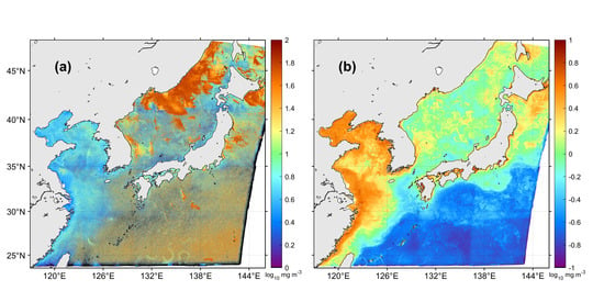
The Geostationary Ocean Color Imager (GOCI) is the world’s first geostationary optical satellite sensor dedicated to ocean observations (as opposed to meteorological observations). Since its launching in 2010, it has produced ocean color data over the seas around the Korean Peninsula, with an unprecedented high temporal resolution of 1 h and eight bands from visible to near infrared (Figure 1a) [1]. It has contributed significantly to various research fields by taking advantage of geostationary orbit, enabling time-based observation during the daytime [2,3,4,5]. In particular, the ocean-atmosphere interactions or the responses of marine ecosystems over short-term periods can be studied using GOCI chlorophyll-a (chl-a) concentration data [6]; several polar-orbit ocean color satellites launched previously did not offer this advantage. GOCI is expected to be used not only for investigating short-term variability, but also for mid- to long-term variability studies on the seas around the Korean Peninsula based on the GOCI database accumulated over the past 10 years.
Ocean color data have been reported to have noise errors and diverse problems, including stray light effects from instruments, difficulties in sensor calibration, and failures with atmospheric correction related to contamination from cloud edges, sun glint, whitecaps, and aerosols [7,8,9,10,11,12,13,14,15]. Moreover, these were particularly more conspicuous than other variables in the chl-a concentration products. Similar to previous ocean color satellite sensors such as the Sea-viewing Wide Field-of-view Sensor (SeaWiFS) and Moderate Resolution Imaging Spectroradiometer (MODIS), the level-2 product of the GOCI data also exhibited problems related to error with extremely high values, i.e., up to 1.00 × 10³ times higher than the neighboring values of the background field. Erroneous low-value pixels are also apparent in GOCI data. In GOCI chl-a images, these errors frequently appear as speckle noise in a single pixel, unexpectedly congregated patches, or array-like features; they may be associated with unsuccessful atmospheric corrections caused by factors such as aerosol and cloud contamination or instrumental-related artifacts such as slot-related stray light (e.g., [16]). Unlike traditional ocean color sensors, the target area of GOCI is covered by 16 consecutive acquisitions in 4 × 4 slots, which tends to induce inconsistencies and noise between the adjacent slots in GOCI products (Figure 1b) [17,18]. The Korea Ocean Satellite Center/Korea Institute of Ocean Science and Technology (KOSC/KIOST) recently updated the standard GOCI atmospheric correction by modifying the aerosol model and applying a vicarious calibration [19,20]. However, although the overall quality of the database was improved owing to this update of the atmospheric correction, it still contains substantial noise errors. The errors in the chl-a concentration image need to be processed properly to enhance the reliability of the data for scientific analysis.
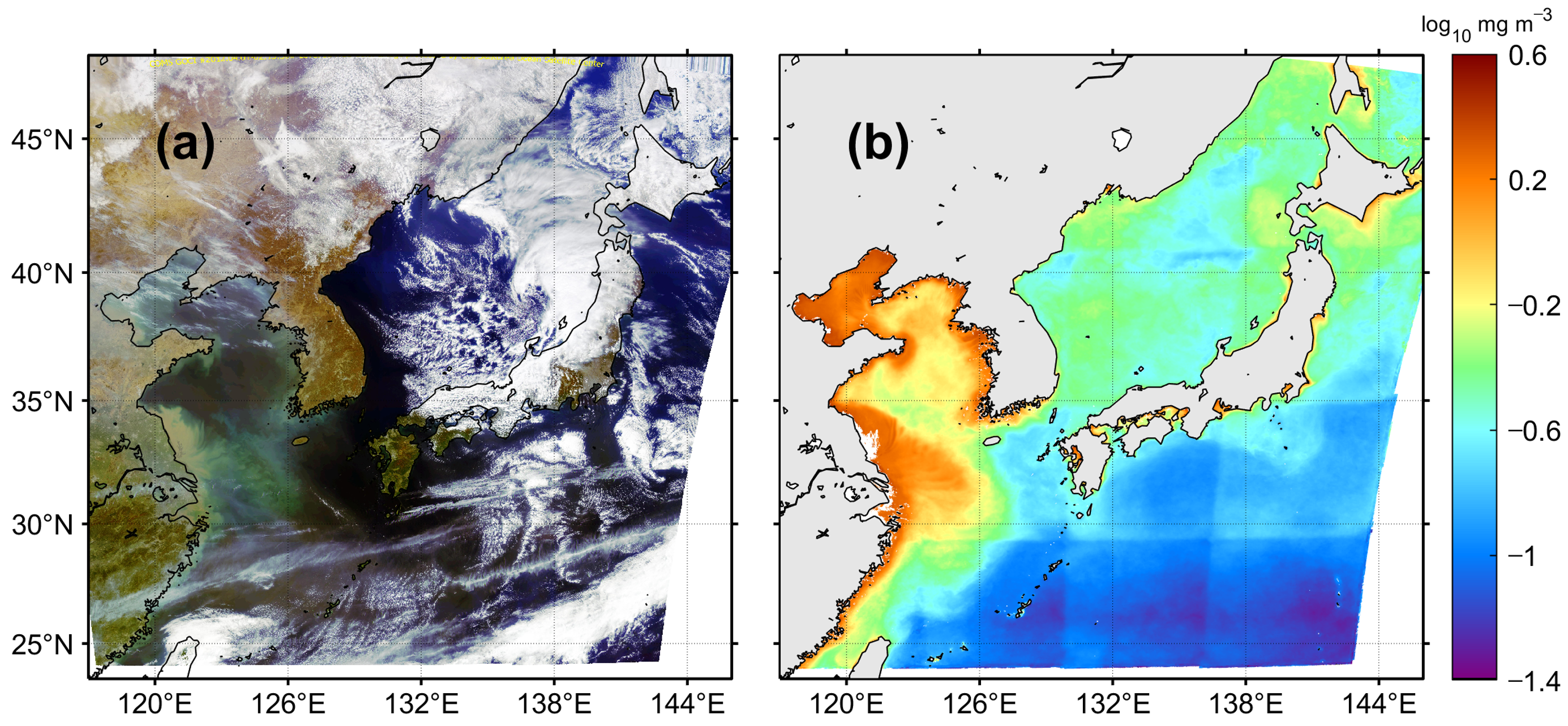
Methodologies for the removal of erroneous pixels in ocean color images has been proposed based on the spatial and temporal distribution of the data values [8,9,16,21,22]. Most of them were based on smoothing scheme or thresholds to eliminate speckles in the chl-a concentration images; however, this is mainly advantageous when the distribution of the image background field does not change much, or when the speckle values are extremely high compared with the surroundings. Ocean color properties in the GOCI observation area vary remarkably from oligotrophic water, known as Case 1, to very turbid water, known as Case 2, as shown in the monthly climatology map in April (Figure 1b). The general distribution of chl-a concentration values in the GOCI coverage was divided into three groups: the Northwest Pacific, East Sea, and Yellow Sea from an image of chl-a concentration (Figure 2). The three regions each tend to have a unique distribution of chl-a concentration values in terms of number density. However, the three regions have some portions with significant overlapping, as shown in Figure 2. In particular, the East Sea is a mixture of several optical properties based on large spatio-temporal variability of chl-a concentration caused by large seasonal variability, strong spatial chl-a fronts, and complicated mesoscale features [23,24,25,26,27]. These wide ranges of variabilities of bio-optical conditions make it difficult to detect pixels of abnormal value properly. Thus, a more advanced methodology should be developed.
Recently, deep neural networks (DNN), have been rapidly developed to be utilized for ocean color satellite image processing, such as image classification, target detection, and prediction of oceanic features [28,29,30]. One of the most significant improvements of the deep-learning methods may be found in automated feature extractions, which were previously performed manually. The DNN were built as a hierarchy of data representations dealing with spectral information for each pixel. Semantic segmentation is the task of assigning each pixel of an input image to a specific class, which is an area where deep-learning has shown particularly good results. Additionally, they can effectively identify substantial noises, performing well under different background image conditions in remote sensing. DNN-based ocean color algorithms can also be adopted for operational and near-real-time satellite observations thanks to their high speed and accuracy [31,32]. Therefore, the deep-learning method can be applied to improve the quality of GOCI variables by eliminating potential noises.
The objectives of this study are: (1) to identify the spectral characteristics of erroneous pixels in the GOCI chl-a concentration images, (2) to develop a detection algorithm for chl-a speckles based on the DNN method, (3) to compare the monthly composites prior to and post the speckle removal procedure using GOCI chl-a data for six years from 2012 to 2017, and (4) to verify the capability of the developed DNN algorithm for erroneous pixel removal procedures.
2. Data and Methods
2.1. Geostationary Ocean Color Imager (GOCI) Data
GOCI level-2 remote-sensing reflectance (λ, sr−1), chl-a concentration image, and flag information from 2012 to 2017 were used for detection of erroneous pixels in the chl-a concentration images. These data were calculated from level-1B data by atmospheric corrections based on GOCI data-processing system (GDPS) 2.0 of the KOSC/KIOST. The GOCI sensor has six visible bands centered at λ = 412, 443, 490, 555, 660, and 680 nm and two near infrared (NIR) bands centered at λ = 745 and 865 nm. To estimate chl-a concentration using data, the GDPS suggests an empirical ocean chl-a algorithm for GOCI (OC3G) by using three bands:
where CHL represents the chl-a concentration (mg m−3) and the coefficients from to are the empirically regressed coefficients of 0.0831, −1.9941, 0.5629, 0.2944, and −0.5458, respectively. The GOCI data has a spatial resolution of 500 m × 500 m and a high temporal sampling capability of eight times per day from 9:30 AM to 4:30 PM local time (KST) [1,33]. In this study, we used all hourly databases of GOCI data for six years, from 2012 to 2017 including a total of 17,522 chl-a concentration images.
2.2. Speckle Detection Based on Deep Neural Network Approach
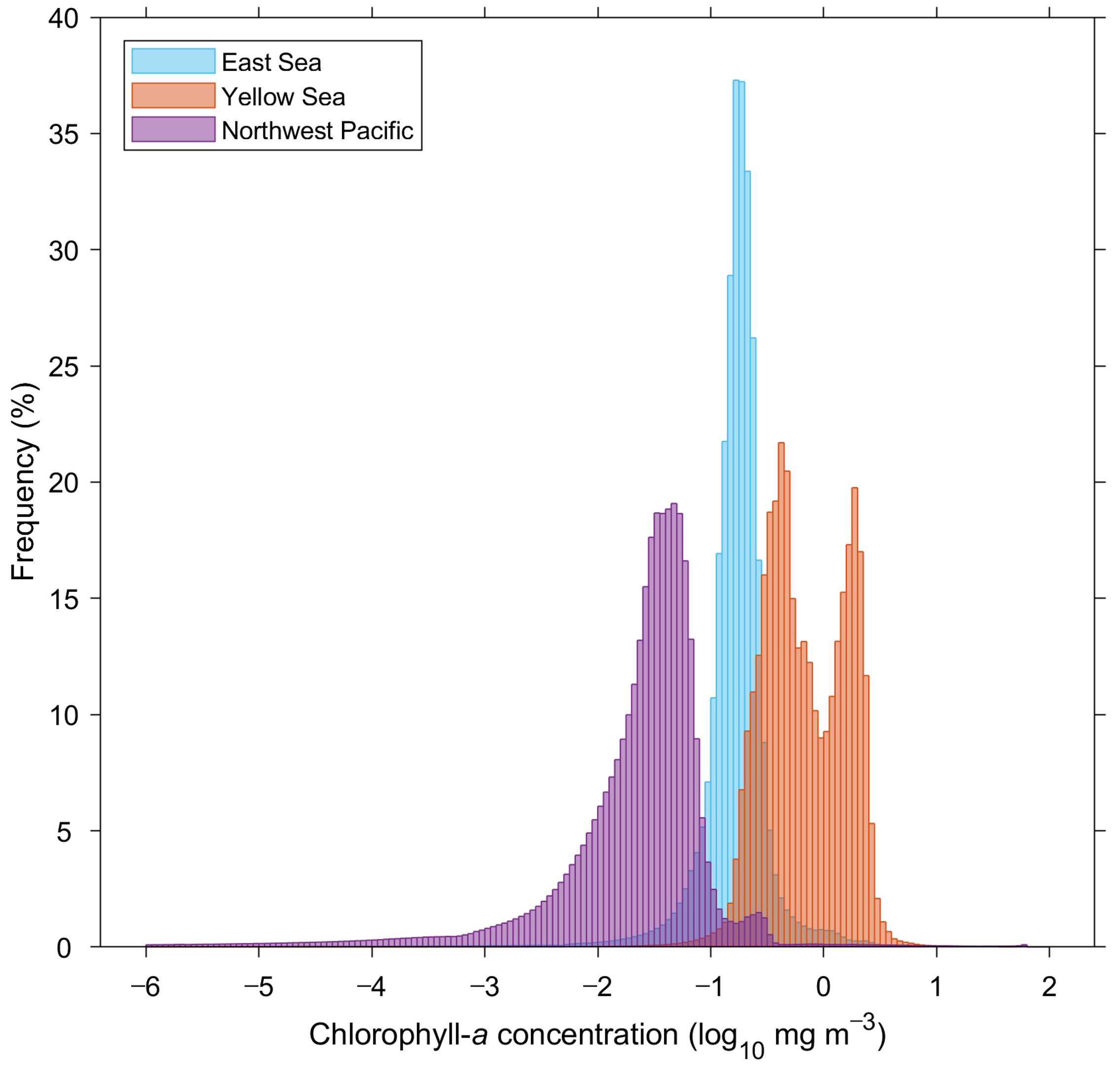
We developed a neural network algorithm based on a deep-learning model to classify the pixels into three categories: normal, abnormally high, and abnormally low values of chl-a concentration in a GOCI image. In this study, a multilayer feedforward neural network (MFNN) was utilized through DNN with three hidden layers. For the MFNN presented in this work, a back-propagation learning technique with a Levenberg-Marquardt optimization, also known as the damped least-squares method, was implemented [34,35,36,37]. The input layer comprised 11 datasets of (λ) of eight bands, a chl-a concentration image, a 3 × 3 median filtered chl-a concentration image, and monthly climatological data on chl-a concentration that were used to consider the spectral shape of each pixel and the spatiotemporal variability of the field (Figure 3). The monthly climatological chl-a concentration data were acquired by taking an average of level-2 chl-a concentration data over the six years from 2012 to 2017 for each month after applying a median filter within a 3 × 3 window for smoothing. Each input layer received data from an entire GOCI image, with pixel sizes of 5685 × 5567, in latitudinal and longitudinal directions. The output layer returned a pixel-wise confidence metric from 0 to 1 continuously for the classes being processed. Pixel-wise calculations in the model, which are based on the spectral characteristics and spatiotemporal properties of chl-a, enable the detection of both sporadic and patch-type errors.
2.3. Construction of Dataset
To reduce the range of calculations required during the MFNN process as well as the resulting uncertainty, the input data were conditionally masked using the following criteria. Various level-2 flags were rendered as invalid pixels to discard low-quality data, that were in turn clearly marked with flag information including divergence from the iterative atmospheric condition, a high aerosol concentration, negative normalized water-leaving radiance, negative Rayleigh-corrected NIR, turbid water, a high possibility of pixel contamination, and an invalid condition to derive chl-a, with zero or empty values. After the flags were applied, the pixels were rejected from the subsequent process when any of the values of 443, 490, and 555 nm used in the chl-a retrieval algorithm were negative and when (660) was infinite, these were also invalid pixel conditions for that were not filtered out by flags. To prevent overfitting errors during the development of the algorithm, the input data were randomly divided into three groups as follows: 70% for training, 15% for validation, and 15% for testing as a completely independent dataset for network generalization. The training set was used to compute and update the neural network model. The validation set was not involved in the training process; instead, it was used to determine the optimal learning. The model stopped updating when the minimum error was reached in the validation set. The test set was used to evaluate the final performance of the model after the training process was completed. The training, validation, and testing datasets were constructed from a total of 72 chl-a concentration images using a 1:30 PM (KST) image obtained on the 15th of each month during 2012–2017, to utilize the maximum possible chl-a spatiotemporal variability in the study area. Actual (target) data, that defined the pixels with abnormal values compared to the normal pixels, were determined based on the threshold scheme described in previous research on speckle removal in ocean color images [14]. Pixels detected as speckles were divided into abnormally high- and low- value pixels using the ratios between the chl-a concentration image, its 3 × 3 median filtered image, and the monthly climatology chl-a concentration image; the thresholds of 1.3 and 0.7 were provided for high and low values, respectively, prior to the application of the deep-learning procedures.
2.4. Statistical Errors
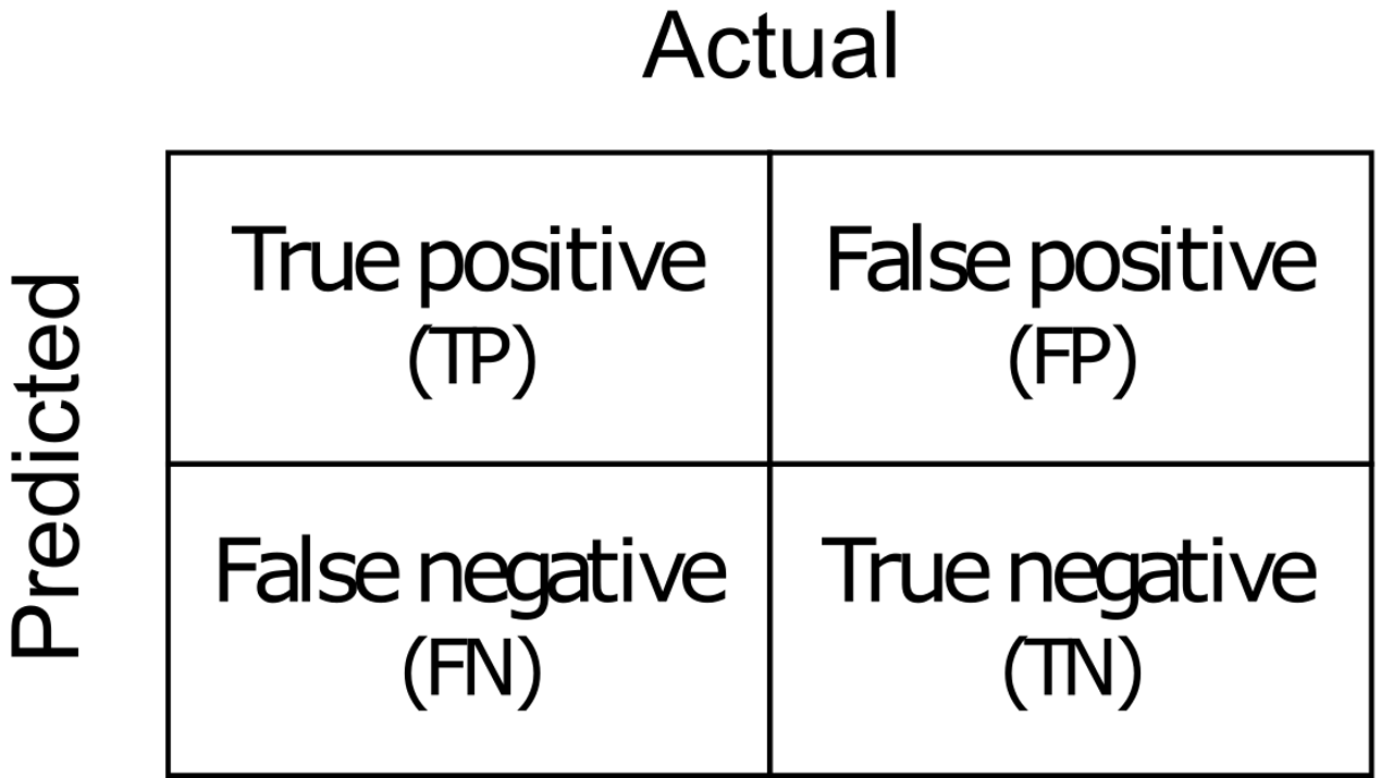
The performance of the MFNN model was quantitatively evaluated in terms of the accuracy, precision, and sensitivity based on a confusion matrix (Figure 4). The accuracy of the model () in equation (2) gives the overall accuracy of the model. This means that it is the fraction of the total samples that were correctly classified by the algorithm on the basis of the pixel classification among the true positive (TP), true negative (TN), false positive (FP), and false negative (FN), where the positive and the negative signify the target pixel and not target pixel of each class, respectively. To calculate the accuracy, the following Equation (2) was used:
The sensitivity of the model () identifies the fractions of all positive samples correctly predicted as positive by the model given by Equation (3):
The precision of the model () indicates what fractions of predictions as a positive class were actually positive, as presented in the following Equation (4):
F-score of the model () is calculated from the and the to find the optimal balance between the two as the harmonic mean of Equation (5):
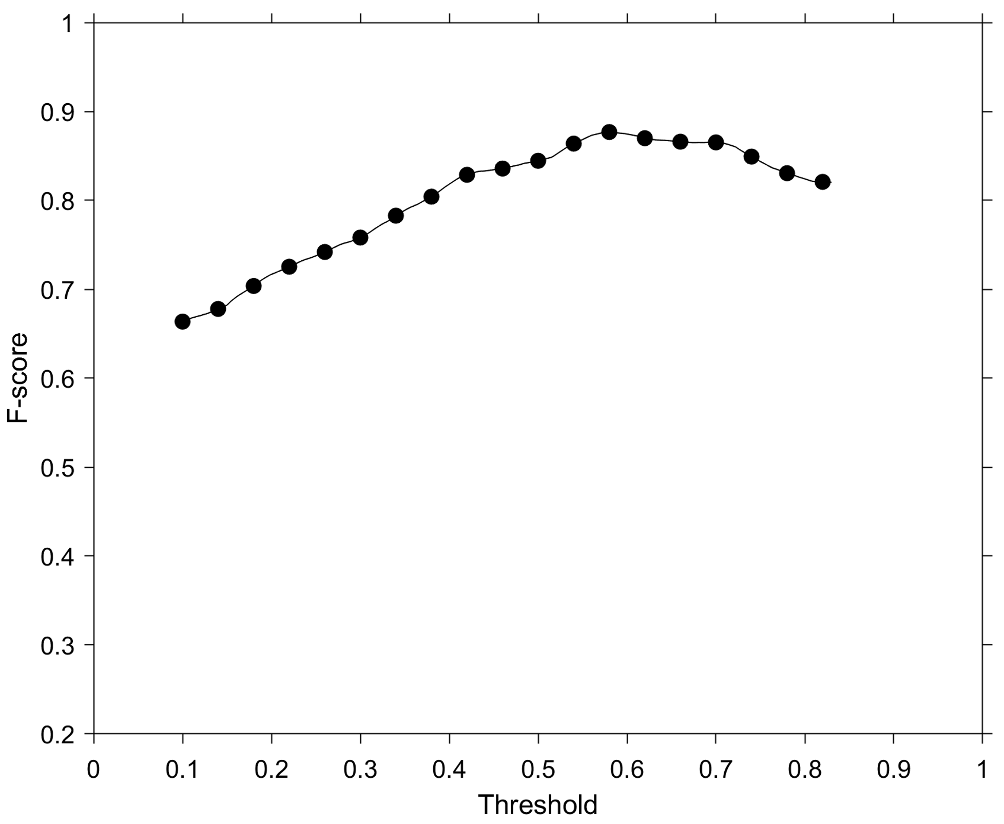
All segmented values of the model near 1 show better segmentation. The output of the MFNN algorithm is an erroneous pixel confidence metric ranging from zero to 1; therefore, a threshold value must be determined for classification. In this study, we used a fixed threshold value of 0.6 for the output classes, when evaluating the models.
3. Results
3.1. Speckles from Annual Maximum
The annual maximum value of chl-a and the month with the annual maximum were computed for each pixel by using all the chl-a concentration images for the year 2015 to investigate the appearance of abnormally high speckles per year. Figure 5a shows the spatial distribution of yearly maximum values randomly distributed in the forms of salt and pepper noises or patched chl-a concentration. The enlarged area (Figure 5b), marked in the red box in Figure 5a, also reveals a discontinuous noise and patch type with abnormally high chl-a concentrations. These unusual features are notably different from the general distribution of normal chl-a concentration values in space, as shown in the monthly climatology map of Figure 1b. The annual maximum values in the East Sea and northwest Pacific are higher at approximately 60 and 40 mg m−3, respectively, which are even higher than the highly turbid Case 2 water of the Yellow Sea in Figure 5b. Furthermore, they are much higher than the April monthly climatology distribution, shown in Figure 1b, for the spring bloom season of phytoplankton in the East Sea [4,38,39,40]. The distribution of the month with the annual maximum in each region also tended to be very sporadic and locally patched (Figure 5c). In the northern part of the East Sea, there are high chl-a patches, mainly observed in winter and early spring (December to March) (Figure 5c). This is not the local maximum bloom season or at the beginning of bloom [4,38,39,40]. Therefore, it is unlikely that an intensity bloom of up to 60 mg m−3 will appear in the northern East Sea during winter or early spring.
3.2. Abnormal Chlorophyll-a Features around Clouds
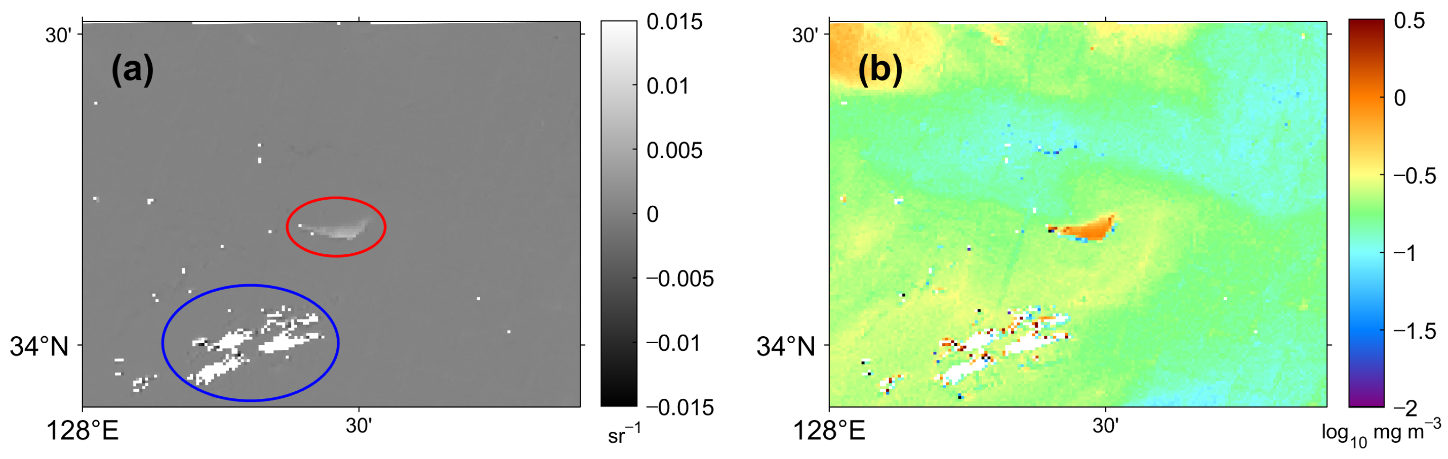
There are many types of cloud passing over the seas around the Korean Peninsula, depending on the local atmospheric and oceanic conditions. The GOCI instrument takes 8-band images sequentially for 2 min at each pixel in a slot and approximately 30 min for all pixels within the entire region in total. During a 2-min period, the locations of the clouds may be shifted from their original locations between the first and last bands, which generates time differences between each band observation, resulting in a cloud pixel registration error. Unlike the interior thick and large patched cloud pixels with a high spatial uniformity of reflectance, the boundaries of the clouds are affected by the rapid changes in the reflectance values for each GOCI band. The cloud pixel registration error can constitute an inappropriate band spectrum and may produce abnormally high- or low- value errors around the cloud edges. Thin or small fragmented clouds, by contrast, are not likely to be detected during the atmospheric calibration process. If clouds are not properly classified as cloud pixels, the pixels may retrieve abnormal chl-a values owing to higher reflectance than their surroundings originating from the ocean.
The grayscale image of (555) shows bright pixels of high reflectance considering clouds in the central (red ellipse) and lower-left (blue ellipse) areas of Figure 6a. At the location of the blue ellipse in Figure 6a, abnormally high and low chl-a values appear around the boundary of the scattered clouds, as marked in white pixels in Figure 6b. The scattered abnormal values along the cloud patches are distinguished from the background chl-a concentrations at approximately 0.4 mg m−3 (~−0.4 on a log10 scale). Other forms of erroneous values can be found in Figure 6b from the position, marked in the red circle, in Figure 6a. Relatively high chl-a values appear in the type of a small triangle-like patch, which is approximate 6-times higher than the surroundings. These abnormal distributions of the chl-a values are likely due to some failures in the cloud detection.
3.3. Dual Structure of Speckles
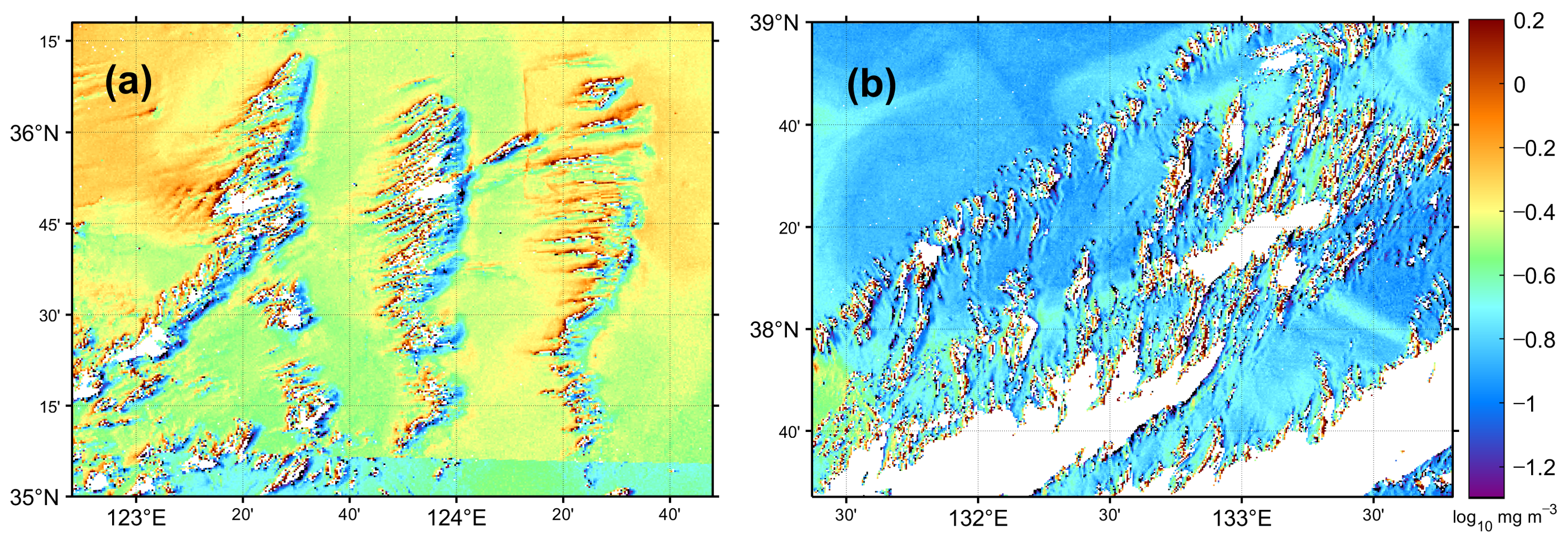
Figure 7 represents other examples of erroneous pixels near various types of clouds in chl-a concentration image on 3 June 2015. One intriguing feature of Figure 7a is the appearance of a dual structure of abnormal chl-a values with higher values aligned with unexpected lower values across the cloud pixels, as marked in white. There are three arrays of elongated clouds across which two arrays of higher chl-a concentration values on the left side and lower chl-a concentration values on the right side are detected. This trend is also apparent near the patchy-type clouds between two elongated cloud arrays in the lower portion of Figure 7a. More systematic features, with the dual structure, were detected from the scattered clouds in Figure 7b. Both higher and lower values appear systematically near the clouds except for the pixels inside the clouds illustrated in white. Such structures had remarkably different values of chl-a concentration, as compared with the background chl-a image showing spatially consistent variations with high uniformity.
All of these features seemed to be related to the failure in cloud detection due to the movement of the clouds during GOCI observations within a slot of 2 min. When these features are given into a composite procedure to produce a monthly map, the resulting composite will bring errors with spatially much less uniformity of chl-a values. Water leaving radiance around shallow coastal areas disturbed by seafloor reflectance and stray light originating from land also have the potential to cause incorrect atmospheric correction results. These complex optical properties may influence the retrieval of low chl-a concentrations compared to background images near the island and mainland. In addition, high-altitude aerosol conditions around cloud edges are likely to be different from the aerosol type of the background field especially in the open ocean, which makes it difficult to choose the proper aerosol model in the atmospheric correction procedure. This type of improper selection in the aerosol models may also lead to the emergence of an unexpected low chl-a concentration distribution [16]. Thus, the spectral characteristics of such erroneous pixels should be investigated. The following section deals with the spectrum with respect to the wavelengths corresponding to the GOCI bands.
3.4. Spectral Characteristics of Speckles
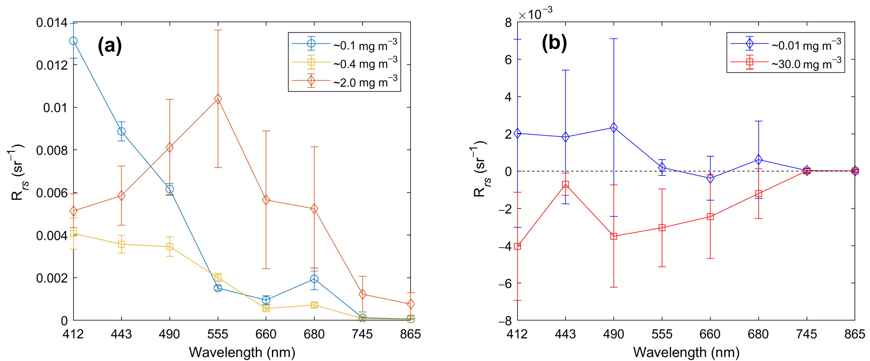
To examine the spectral characteristics of the speckles, the values of the speckles and normal pixels were averaged for each GOCI band, as shown in Figure 8. Normal pixels that retrieve proper chl-a concentration values have been revealed to have spectral patterns, as shown in Figure 8a. Each average spectral shape was obtained from 30 contaminated pixels in the Northwest Pacific, East Sea, and Yellow Sea, respectively in 3 June 2015, as representative optical types from oligotrophic to turbid water. The GOCI spectral signatures averaged over three different ranges of chl-a concentration, 0.1 mg m−3 and 0.4 mg m−3 illustrate the decreasing tendency of with respect to wavelengths. In the range of approximately 2.0 mg m−3, the values tended to increase from 412 nm to reach a peak at 555 nm, subsequently decreasing to the 865 nm wavelength. The shapes differ depending on phytoplankton, colored dissolved organic matter (CDOM), or other substances in seawater. Previous studies have mentioned that the spectral dependency for the different chl-a concentrations groups show that the shapes of the spectra change from a blue-wavelength peak to a green-wavelength peak with increasing chl-a concentration [41,42].
In contrast to normal pixels with overall patterns in Figure 8a, abnormally high and low chl-a concentrations had more flattened shapes as a function of wavelengths (Figure 8b). Unlike the normal pixels, values of 555 and 660 nm were close to zero with very small positive or negative of pixels with very low chl-a concentration of approximately 0.01 mg m−3. The ratio between small values in the green band ((555)) and the large value in the blue band ((443), (490)) may induce extremely low chl-a concentration due to the constant , which has a value of –1.9941, in the OC3G algorithm (Equation (1)). Pixels with very high chl-a concentration of 30 mg m−3 average, suspected as speckle error, show unexpected negative values in all visible bands except for the NIR 745 and 865 nm bands (Figure 8b). Among them, (443) is the closest to 0, so the absolute value of (443) is the smallest. In this case, contrary to the normal values, the retrieval of chl-a concentration according to Equation (1) can be amplified owing to the small value of (443).
3.5. Implementation of Multilayer Feedforward Neural Network (MFNN) Model
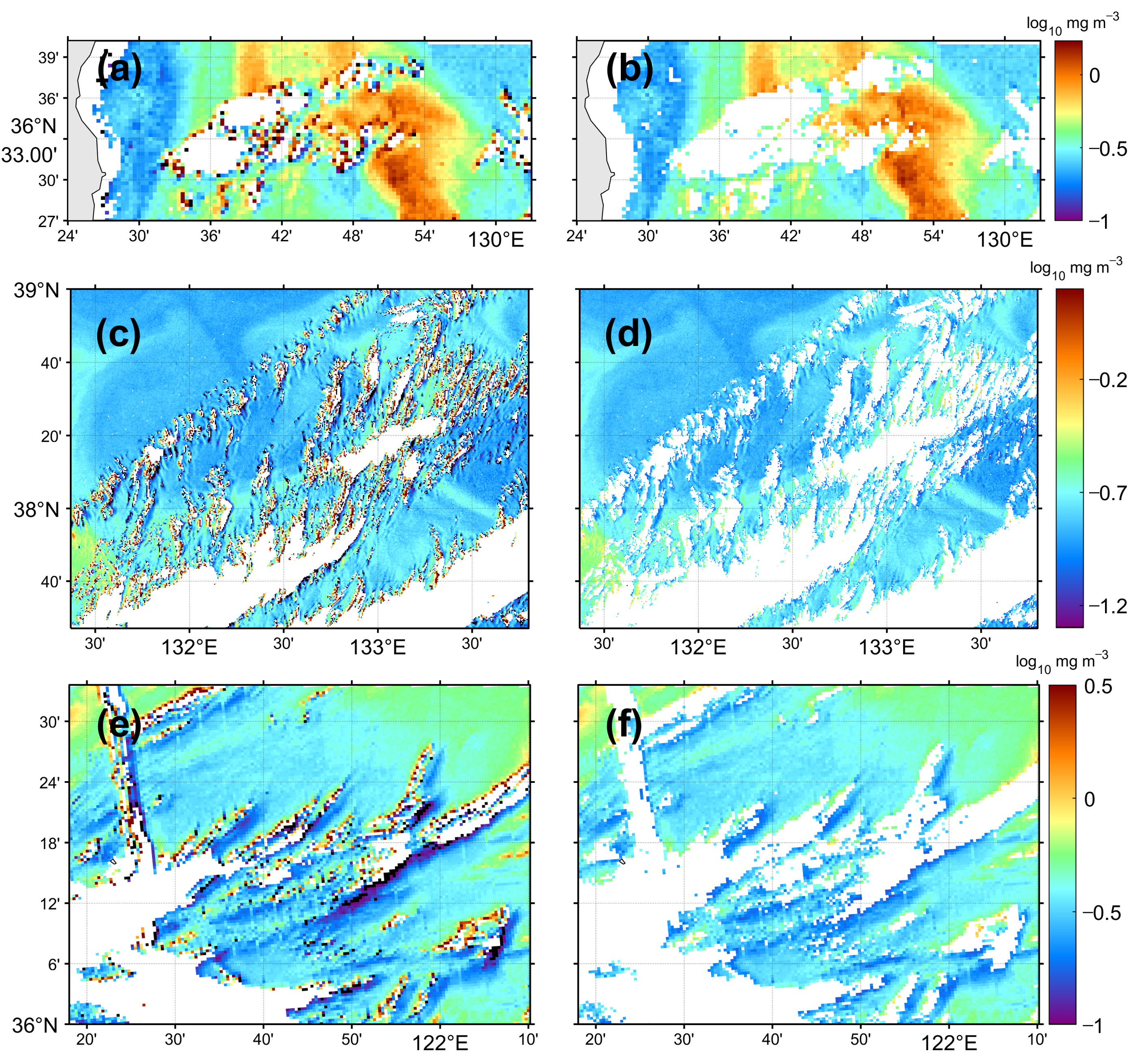
The results of applying the deep-learning model removing the erroneous pixels in individual level-2 chl-a images are presented in Figure 9. Figure 9a shows unexpected speckles along the boundary of cloud patches crossing the narrow upwelling area off the coast of the East Sea at 13:30 KST on 3 June 2015. This might be related to the movement of the clouds over a few minutes within a relatively short time of the sensor observation period. The speckle values are not constant; they are randomly distributed, with values that are spatially dominant compared with neighboring pixels a short distance from the cloud boundary. Figure 9b shows the disappearance of the erroneous pixels, marked in white, as a result of the MFNN model. Considering that the high chl-a concentrations bloom occurred during extensive upwelling events in summer, chl-a values over 1 mg m−3 around the cloud patches were not classified into the speckles. Figure 9c,d show another arbitrary example of the removal procedure applied to complicated clouds with small-scale elongated structures. The background chl-a field is relatively spatially homogeneous, mostly distributed around 0.2 mg m−3, while highly speckled chl-a values were detected around the cloud edges (Figure 9c). After the deep learning method was applied, abnormal speckle pixels were excluded with a high performance as shown in Figure 9d.
The spatially dominant pattern is a dual structure with a pair of high and low chl-a values on either side of an elongated cloud patch (Figure 9e). On one side of the cloud patch, the distribution of chl-a concentrations appears at approximately 3 mg m−3 while on the other side this occurs at almost 0.1 mg m−3. The low chl-a values, indicated in purple, seem to not have originated from a natural chl-a distribution in the highly turbid Yellow Sea. Figure 9f shows the result of applying the deep learning algorithm to remove abnormal pixel with both significantly high and low values. As shown in Figure 9e,f, both types of pixel were properly removed although some pixels with lower values still remained near the edge of clouds. This region corresponded to the cloud shadow region parallel to the pixels with abnormally high values. One potential cause of this is that the spectral shape of the low-value pixels had a relatively high similarity to those of ordinary pixels, as indicated in Figure 8. However, the differences in the chl-a values for the low-value pixels and the neighboring normal pixels are negligible at less than order of 10−1. Images of chl-a concentration on a logarithmic scale tend to visually exaggerate any differences, particularly for values lower than 0.1 mg m−3. Given this, the present method is believed to remove both erroneous values appropriately.
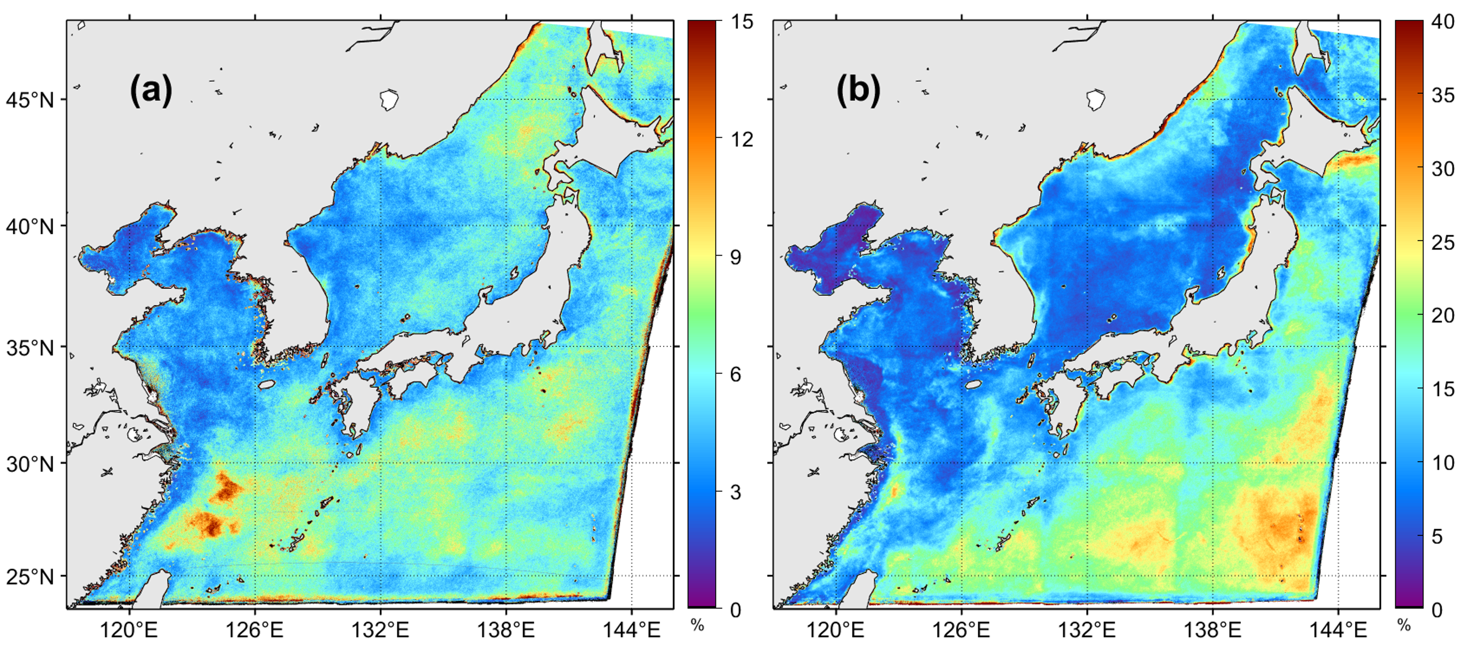
The frequency distribution of the erroneous pixels estimated from the speckle-removal process was obtained as a percentage of the total chl-a observations in 2015 (Figure 10). The frequency of high-value speckles was up to 15% of the total chl-a observation in the entire research area; speckles were frequently observed in the following order: the Yellow Sea (~3%), East Sea (5–10%), and Northwest Pacific (>10%). High-value speckles were observed more often in the eastern region than in the western area of the East Sea. The low-value speckle frequency was up to 40%, which was greater than that of high-value speckles in the entire area. Low-value speckles appeared much more frequently in the Northwest Pacific than in the Yellow Sea and East Sea. One of the interesting features is that the low-value speckles tended to appear more often toward the right side of the slot and lower latitudes, which is evident in the Northwest Pacific. The presence of both high- and low-value speckles at a high frequency in the Northwest Pacific could be attributed to the characteristics of the clouds passing over the Northwest Pacific and atmospheric conditions such as aerosol distribution being different from those of other seas in the study area.
3.6. Effect of De-Speckled Chlorophyll-a Concentration Data on Composite Field
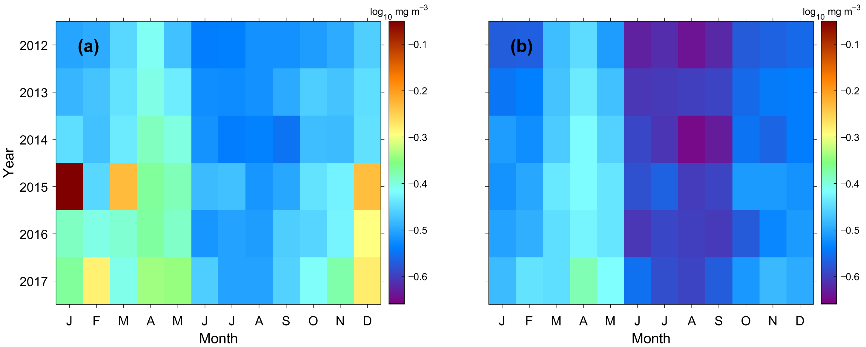
To show the effect of the erroneous speckles in the chl-a concentration of monthly composite, the monthly mean chl-a concentration before reprocessing was compared with the data after the removal algorithm in the study area from 2012 to 2017 (Figure 11). In the month-year plot of chl-a concentrations without applying the speckle removal procedure, the highest chl-a concentrations during the spring bloom of phytoplankton are only weakly apparent in April and May (Figure 11a). In particular, the monthly mean values of chl-a concentrations are abnormally higher in January and March 2015 than in other months. In the period of every December from 2015 to 2017 corresponding to a fall bloom, the chl-a concentration values are much more prominent than those of the spring bloom. In summer, the mean concentration values are significantly lower than in other seasons. The overall mean value of chl-a concentration before reprocessing ranges from 0.28 to 0.89 mg m−3. On the other hand, after the algorithm was applied, the year-month plot shows a remarkable change in the chl-a concentration variability. It exhibits obvious seasonality, as shown in Figure 9b. Seasonal variations in the chl-a concentration indicate a typical pattern with dominant spring blooms from March to May and a relatively weak fall bloom as disclosed by previous studies on the seasonal variability of chl-a in the seas around the Korean Peninsula [27,40]. The variations of the mean concentrations are reduced to a small range from 0.22 to 0.45 mg m−3, which is a narrower range as compared with the range before correction. The decreasing rate amounted to 67% in January 2015.
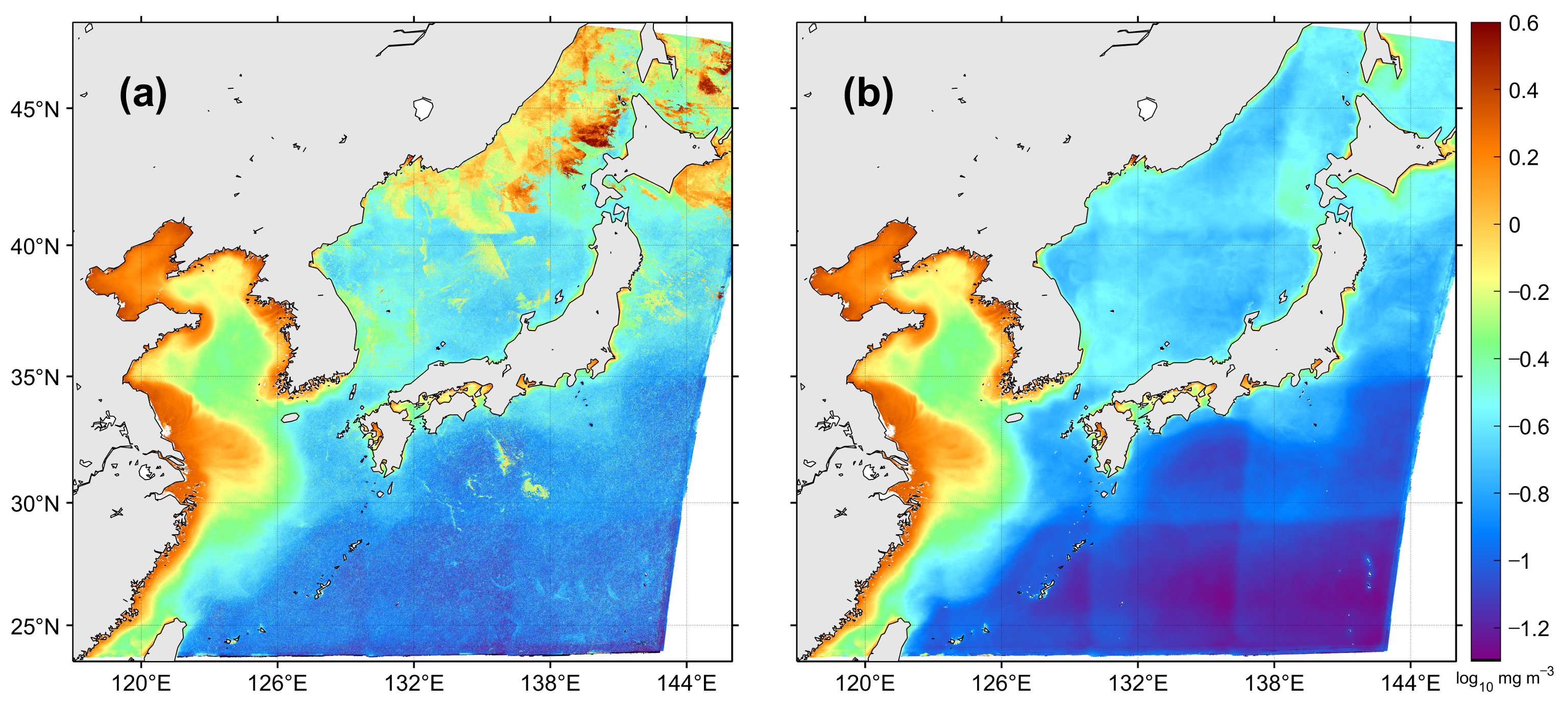
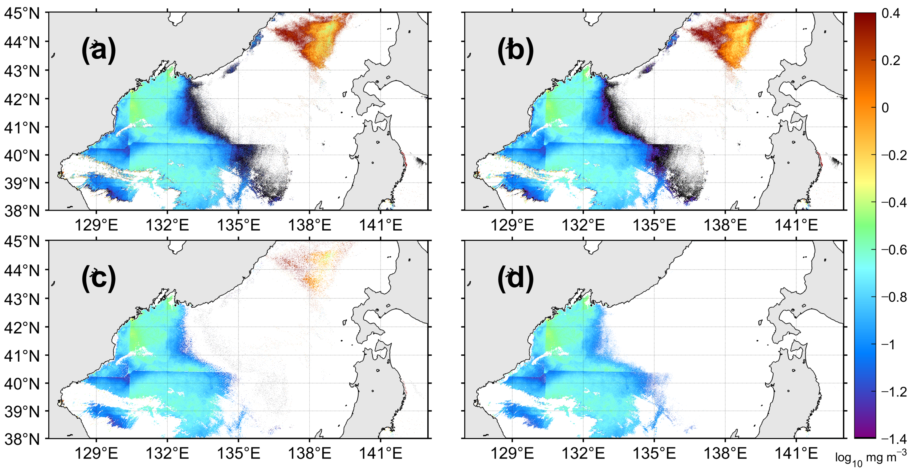
Figure 12 shows the dominant change in the yearly composite map of 2015 before and after the erroneous pixel removal procedure. Many single dots and patches with higher chl-a concentrations than background field appear over the entire yearly map, particularly in the Northwest Pacific and the East Sea prior to the speckle-removal procedure (Figure 12a). However, the reprocessed yearly composite map reveals detailed surface spatial structures of chl-a in 2015, which had been hidden by erroneous values of scattered speckles and patches (Figure 12b). For instance, a mesoscale eddy-like feature appears as a circular shape with chl-a values about 0.3 mg m−3 (−0.5 on a log10 scale) at about 36°N in the far-offshore region of the East Sea. In addition, relatively high chl-a concentrations are comparatively well represented along the coastlines of Russia, Korea, and Japan. High chl-a distribution in the Yellow Sea of case 2 water were also well preserved instead of being classified as abnormal values during the speckle-removal process. As mentioned previous, slot-related spatially distinctive discontinuity in the GOCI image have been reported [17,18], however, the effect of the slots is not clearly distinguished in Figure 12a due to high chl-a speckles around the slot boundaries. In contrast, Figure 12b illustrates the slot-related differences along the slot boundaries after the removal of abnormal values, which is more evident in the Northwest Pacific region of case 1 water with low chl-a distribution. This study did not cover the slot issue in further detail. These results confirm the good performance of the speckle removal model for the level-3 composite procedure.
3.7. Validation
The output layer of the MFNN model is a confidence metric, and thus the threshold for decision boundary of each class should be considered to maintain the high performance of the model. Over all valid pixels in a dataset, the relationship between the threshold value and averaged of output classes was investigated (Figure 13). As the threshold was increased from 0.1 to around 0.6, the tended to increase from 0.66 to 0.87. As a result of checking the , the threshold is assigned to 0.6 for output class. To validate the effectiveness of the proposed method, a confusion matrix is obtained using a given threshold of 0.6 for each output class (Table 1). The statistical parameters are higher than 0.85 for all classes of the model output, as shown in Table 1. In particular, the accuracy for the low chl-a value class is over 0.9, which is the highest among the three classes.
4. Discussion
As indicated by the results, the characteristics of speckles included randomly scattered or aggregated patches. The potential causes of the appearance of the noise errors can be understood primarily in terms of the problematic values related to atmospheric correction. Water vapor is known to contribute to the creation of the problematic spectral shape of the values. In the atmospheric correction procedure of GOCI data, it is somewhat difficult to consider the effect of water vapor correctly using only bands of GOCI, as this requires additional bands at 6.72, 8.55, and 12.0 μm to discriminate high-, medium-, and low-moisture conditions [43]. Although the GOCI atmospheric correction algorithm considers the moisture distribution from other atmospheric model, detailed information on water vapor is difficult to obtain under near real-time conditions. Such an imperfect atmospheric correction is liable to produce an invalid value for each band [19].
Other potential causes may originate from the cloud contamination, as evident from the appearance of many erroneous pixels at the edges of the clouds. The movement of clouds between observations of the eight GOCI bands over each slot for 2 min causes a spatial shift in the cloud boundary in a single image. Therefore, it is difficult for the atmospheric correction procedure for the GOCI to produce the appropriate values around clouds. One of the easiest ways to remedy this is to remove all pixels with weakly negative values or values extremely close to zero in the procedure to prevent speckles. However, those values do not necessarily provide erroneous chl-a concentrations; they could in fact produce normal chl-a values. Another simple way to counter the error problems is to apply all flags in the chl-a image. However, this can mask a very wide range of conditions that make up not only the noise errors but also the actual bloom itself. Such limitations emphasize the importance of the deep-learning approach.
To compare the general arithmetic algorithms and neural network model, in this study, a 3 × 3 median filter, a threshold method, and our MFNN model were applied to a GOCI chl-a image on 13 January 2015 (Figure 14a). The 3 × 3 median filter was effective in smoothing the spatial distribution as a whole and eliminating isolated problematic pixels; however, it was quite limited in detecting problem pixels in the form of a patch located in the northern area of the East Sea as shown in Figure 14b. The threshold method was based on the ratio between the standard deviation and the mean within a 3 × 3 window with a threshold value of 0.3, for detecting problematic pixels. The threshold method showed better performance in terms of detecting erroneous pixels than the median filter (Figure 14c). However, the interior of the high chl-a patch was not detected owing to its spatial uniformity, which was even lower than the plain values of the western area. The image-applied MFNN model proposed in this study performed well for patch-type errors as well as cloud edges with low values. The threshold method eliminated abnormal pixels by 31.5% of the total number of original pixels in Figure 14a (Figure 14c). In contrast, the MFNN method exhibited high performance capability with regard to the abnormal pixel removal by eliminating 45% of the original pixels (Figure 14d). Previous studies have reported the high performance of the threshold-based scheme for removal speckles in ocean color images [14,16]. The accuracy obtained from the confusion matrix of the threshold method based on the spatial uniformity within 3 × 3 pixels was 91.7% for the image obtained on 13 January 2015 (Figure 14). This accuracy value is quite high and similar to the 92.0% accuracy of the MFNN method for the same image. However, despite the high accuracy of the threshold scheme, a few speckles can remain and may affect the composite field of chl-a images.
The effectiveness of DNNs have been proven within a wide range of neural network applications [44,45]. Although the computational complexity of DNNs may require broader adoption in real-time as well as power-efficient facilities to train the model, once trained it has greater efficiency than general arithmetic algorithms (e.g., [46]). Assuming an algorithm is used that detects a value greater than a threshold as determined based on the ratio between the mean and the standard deviation within a particular window size, the time taken to process the single GOCI image is 103 times higher than the time taken by the MFNN algorithm in this study in the case of non-parallel processing. Therefore, it is expected that the DNN method can contribute to the preliminary processing of GOCI data by removing the erroneous pixels with respect to efficiency and accuracy.
5. Conclusions
The GOCI has observed ocean colors at unprecedented temporal and spatial resolutions in the seas around the Korean Peninsula since 2010. A tremendous amount of GOCI data has been accumulated, enough to be utilized in studies on intra-seasonal, seasonal, and interannual variations of diverse oceanic features as well as short-term variations at time scales from hourly to a couple of days. To investigate at long-term time scale, highly accurate time composites of chl-a concentration are of paramount importance. Speckles of extremely high chl-a concentrations randomly appeared in the GOCI images. In this study, the MFNN method was applied to eliminate such erroneous effects from GOCI chl-a concentration images and estimate its capability. The proposed error detection method based on the DNN algorithm was applied to each level-2 image (chl-a concentration) for six years from 2012 to 2017. The monthly maps showed the disappearance of the speckles at a high-performance rate. This study addressed the necessity of a deep-learning methodology to remove erroneous pixels in order to investigate the spatial and temporal variations of fundamental marine ecosystems.
Author Contributions
Conceptualization, K.-A.P.; data processing, J.-E.P.; methodology, K.-A.P. and J.-E.P.; resources, K.-A.P.; data curation, J.-E.P.; visualization, J.-E.P.; writing—original draft preparation, J.-E.P.; writing—review and editing, K.-A.P. All authors have read and agreed to the published version of the manuscript.
Funding
This research was a part of the projects entitled ‘Deep Water Circulation and Material Cycling in the East Sea (20160040)’ funded by the Ministry of Oceans and Fisheries, Korea and was funded partly by the Korea Meteorological Administration Research and Development Program under Grant KMI2018-05110.
Informed Consent Statement
Not applicable.
Data Availability Statement
GOCI data used in this study are available from KOSC/KIOST (http://kosc.kiost.ac.kr/).
Acknowledgments
We thank two anonymous reviewers for providing helpful comments on earlier drafts of the manuscript.
Conflicts of Interest
The authors declare no conflict of interest.
References
- Choi, J.K.; Park, Y.J.; Ahn, J.H.; Lim, H.S.; Eom, J.; Ryu, J.H. GOCI, the world’s first geostationary ocean color observation satellite, for the monitoring of temporal variability in coastal water turbidity. J. Geophys. Res. Oceans 2012, 117. [Google Scholar] [CrossRef]
- Choi, J.K.; Min, J.E.; Noh, J.H.; Han, T.H.; Yoon, S.; Park, Y.J.; Moon, J.-E.; Ahn, J.-H.; Ahn, S.-M.; Park, J.H. Harmful algal bloom (HAB) in the East Sea identified by the Geostationary Ocean Color Imager (GOCI). Harmful Algae 2014, 39, 295–302. [Google Scholar] [CrossRef]
- Yang, H.; Choi, J.K.; Park, Y.J.; Han, H.J.; Ryu, J.H. Application of the Geostationary Ocean Color Imager (GOCI) to estimates of ocean surface currents. J. Geophys. Res. Oceans 2014, 119, 3988–4000. [Google Scholar] [CrossRef]
- Park, J.E.; Park, K.A.; Ullman, D.S.; Cornillon, P.C.; Park, Y.J. Observation of diurnal variations in mesoscale eddy sea-surface currents using GOCI data. Remote Sens. Lett. 2016, 7, 1131–1140. [Google Scholar] [CrossRef] [Green Version]
- Park, K.A.; Lee, M.S.; Park, J.E.; Ullman, D.; Cornillon, P.C.; Park, Y.J. Surface currents from hourly variations of suspended particulate matter from Geostationary Ocean Color Imager data. Int. J. Remote Sens. 2018, 39, 1929–1949. [Google Scholar] [CrossRef] [Green Version]
- Park, J.E.; Park, K.A.; Kang, C.K.; Park, Y.J. Short-term response of chlorophyll-a concentration to change in sea surface wind field over mesoscale eddy. Estuaries Coast. 2020, 43, 646–660. [Google Scholar] [CrossRef]
- Gordon, H.R.; Wang, M. Influence of oceanic whitecaps on atmospheric correction of ocean-color sensors. Appl. Opt. 1994, 33, 7754–7763. [Google Scholar] [CrossRef]
- Hu, C.; Carder, K.L.; Muller-Karger, F.E. Atmospheric Correction of SeaWiFS Imagery over Turbid Coastal Waters: A Practical Method. Remote Sens. Environ. 2000, 74, 195–206. [Google Scholar] [CrossRef]
- Robinson, W.D.; Schmidt, G.M.; McClain, C.R.; Werdell, P.J. Changes Made in the Operational SeaWiFS Processing. SeaWiFS Postlaunch Calibration Valid. Anal. 2000, 2, 12–28. [Google Scholar]
- Hu, C.; Carder, K.L.; Muller-Karger, F.E. How precise are SeaWiFS ocean color estimates? Implications of digitization-noise errors. Remote Sens. Environ. 2001, 76, 239–249. [Google Scholar] [CrossRef]
- Oh, E.; Hong, J.; Kim, S.W.; Cho, S.; Ryu, J.H. Ray Tracing Based Simulation of Stray Light Effect for Geostationary Ocean Color Imager. In Proceedings of the Optical Modeling and Performance Predictions VI, International Society for Optics and Photonics, Society of Photo-Optical Instrumentation Engineers (SPIE), San Diego, CA, USA, 25–29 August 2013; Volume 8840, p. 884006. [Google Scholar]
- Chae, H.J.; Park, K.A. Characteristics of speckle errors of SeaWiFS chlorophyll-α concentration in the East Sea. J. Korean Earth Sci. Soc. 2009, 30, 234–246. [Google Scholar] [CrossRef]
- Hu, C.; Lee, Z.; Franz, B. Chlorophyll a algorithms for oligotrophic oceans: A novel approach based on three-band reflectance difference. J. Geophys. Res. Oceans 2012, 117. [Google Scholar] [CrossRef] [Green Version]
- Park, K.A.; Chae, H.J.; Park, J.-E. Characteristics of satellite chlorophyll—A concentration speckles and a removal method in a composite process in the East/Japan Sea. Int. J. Remote Sens. 2013, 34, 4610–4635. [Google Scholar] [CrossRef]
- Wang, M.; Son, S. VIIRS-derived chlorophyll-a using the ocean color index method. Remote Sens. Environ. 2016, 182, 141–149. [Google Scholar] [CrossRef]
- Lee, M.S.; Park, K.A.; Moon, J.E.; Kim, W.; Park, Y.J. Spatial and temporal characteristics and removal methodology of suspended particulate matter speckles from Geostationary Ocean Color Imager data. Int. J. Remote Sens. 2019, 40, 3808–3834. [Google Scholar] [CrossRef]
- Kim, W.; Ahn, J.H.; Park, Y.J. Correction of stray-light-driven interslot radiometric discrepancy (ISRD) present in radiometric products of geostationary ocean color imager (GOCI). IEEE Trans. Geosci. Remote Sens. 2015, 53, 5458–5472. [Google Scholar] [CrossRef]
- Kim, W.; Moon, J.E.; Ahn, J.H.; Park, Y.J. Evaluation of Stray Light Correction for GOCI Remote Sensing Reflectance Using in Situ Measurements. Remote Sens. 2016, 8, 378. [Google Scholar] [CrossRef] [Green Version]
- Ahn, J.H.; Park, Y.J.; Kim, W.; Lee, B. Vicarious calibration of the geostationary ocean color imager. Opt. Express 2015, 23, 23236–23258. [Google Scholar] [CrossRef] [PubMed]
- Ahn, J.H.; Park, Y.J.; Kim, W.; Lee, B. Simple aerosol correction technique based on the spectral relationships of the aerosol multiple-scattering reflectances for atmospheric correction over the oceans. Opt. Express 2016, 24, 29659–29669. [Google Scholar] [CrossRef]
- Patt, F.S.; Barnes, R.A.; Eplee, R.E.; Franz, B.A., Jr.; Robinson, W.D.; Feldman, G.C.; Bailey, S.W.; Gales, J.; Werdell, P.J.; Wang, M.; et al. Algorithm Updates for the Fourth SeaWiFS Data Reprocessing, NASA Tech. Memo; 2003–206892; Hooker, S.B., Firestone, E.R., Eds.; NASA Goddard Space Flight Center: Greenbelt, MD, USA, 2003; Volume 22, p. 74.
- IOCCG. Guide to the Creation and Use of Ocean-Colour, Level-3, Binned Data Products; Antoine, D., Ed.; Reports of the International Ocean-Colour Coordinating Group, No. 4; IOCCG: Dartmouth, NS, Canada, 2004. [Google Scholar]
- Yoo, S.; Kim, H.C. Suppression and enhancement of the spring bloom in the southwestern East Sea/Japan Sea. Deep Sea Res. Part II: Top. Stud. Oceanogr. 2004, 51, 1093–1111. [Google Scholar] [CrossRef]
- Yoo, S.; Park, J. Why is the southwest the most productive region of the East Sea/Sea of Japan? J. Mar. Syst. 2009, 78, 301–315. [Google Scholar] [CrossRef]
- Park, K.A.; Woo, H.J.; Ryu, J.H. Spatial scales of mesoscale eddies from GOCI Chlorophyll-a concentration images in the East/Japan Sea. Ocean Sci. J. 2012, 47, 347–358. [Google Scholar] [CrossRef]
- Joo, H.; Lee, D.; Son, S.H.; Lee, S.H. Annual New Production of Phytoplankton Estimated from MODIS-Derived Nitrate Concentration in the East/Japan Sea. Remote Sens. 2018, 10, 806. [Google Scholar] [CrossRef] [Green Version]
- Park, J.E.; Park, K.A.; Kang, C.K.; Kim, G. Satellite-observed chlorophyll-a concentration variability and its relation to physical environmental changes in the East Sea (Japan Sea) from 2003 to 2015. Estuaries Coast. 2020, 43, 630–645. [Google Scholar] [CrossRef]
- Lee, M.S.; Park, K.A.; Chae, J.; Park, J.E.; Lee, J.S.; Lee, J.H. Red tide detection using deep learning and high-spatial resolution optical satellite imagery. Int. J. Remote Sens. 2020, 41, 5838–5860. [Google Scholar] [CrossRef]
- Zhu, X.X.; Tuia, D.; Mou, L.; Xia, G.S.; Zhang, L.; Xu, F.; Fraundorfer, F. Deep learning in remote sensing: A comprehensive review and list of resources. IEEE Geosci. Remote Sens. Mag. 2017, 5, 8–36. [Google Scholar] [CrossRef] [Green Version]
- Jeppesen, J.H.; Jacobsen, R.H.; Inceoglu, F.; Toftegaard, T.S. A cloud detection algorithm for satellite imagery based on deep learning. Remote Sens. Environ. 2019, 229, 247–259. [Google Scholar] [CrossRef]
- Doerffer, R.; Schiller, H. The MERIS Case 2 water algorithm. Int. J. Remote Sens. 2007, 28, 517–535. [Google Scholar] [CrossRef]
- Brockmann, C.; Doerffer, R.; Peters, M.; Stelzer, K.; Embacher, S.; Ruescas, A. Evolution of the C2RCC neural network for Sentinel 2 and 3 for the retrieval of ocean colour products in normal and extreme optically complex waters. In Proceedings of the Living Planet Symposium, Prague, Czech Republic, 9–13 May 2016. [Google Scholar]
- Ryu, J.-H.; Han, H.-J.; Cho, S.; Park, Y.-J.; Ahn, Y.-H. Overview of Geostationary Ocean Color Imager (GOCI) and GOCI Data Processing System (GDPS). Ocean Sci. J. 2012, 47, 223–233. [Google Scholar] [CrossRef]
- Bishop, C.M. Neural Networks for Pattern Recognition; Oxford University Press: Oxford, UK, 1995. [Google Scholar]
- Gross, L.; Thiria, S.; Frouin, R. Applying artificial neural network methodology to ocean color remote sensing. Ecol. Modell. 1999, 120, 237–246. [Google Scholar] [CrossRef]
- Chen, S.; Hu, C. Estimating sea surface salinity in the northern Gulf of Mexico from satellite ocean color measurements. Remote Sens. Environ. 2017, 201, 115–132. [Google Scholar] [CrossRef]
- Moré, J.J. The Levenberg-Marquardt algorithm: Implementation and theory. In Numerical Analysis; Springer: Berlin/Heidelberg, Germany, 1978; pp. 105–116. [Google Scholar]
- Yamaguchi, H.; Kim, H.C.; Son, Y.B.; Kim, S.W.; Okamura, K.; Kiyomoto, Y.; Ishizaka, J. Seasonal and summer interannual variations of SeaWiFS chlorophyll a in the Yellow Sea and East China Sea. Prog. Oceanogr. 2012, 105, 22–29. [Google Scholar] [CrossRef]
- Lee, S.H.; Son, S.; Dahms, H.U.; Park, J.W.; Lim, J.H.; Noh, J.H.; Kwon, J.-I.; Joo, H.T.; Jeong, J.Y.; Kang, C.K. Decadal changes of phytoplankton chlorophyll-a in the East Sea/Sea of Japan. Oceanology 2014, 54, 771–779. [Google Scholar] [CrossRef]
- Joo, H.; Son, S.; Park, J.W.; Kang, J.J.; Jeong, J.Y.; Lee, C.I.; Kang, C.-K.; Lee, S.H. Long-term pattern of primary productivity in the East/Japan Sea based on ocean color data derived from MODIS-aqua. Remote Sens. 2016, 8, 25. [Google Scholar] [CrossRef] [Green Version]
- Werdell, P.J.; Bailey, S.W. An improved in-situ bio-optical data set for ocean color algorithm development and satellite data product validation. Remote Sens. Environ. 2005, 98, 122–140. [Google Scholar] [CrossRef]
- Ye, H.; Li, J.; Li, T.; Shen, Q.; Zhu, J.; Wang, X.; Zhang, F.; Zhang, J.; Zhang, B. Spectral classification of the Yellow Sea and implications for coastal ocean color remote sensing. Remote Sens. 2016, 8, 321. [Google Scholar] [CrossRef] [Green Version]
- Ackerman, S.A.; Strabala, K.I.; Menzel, W.P.; Frey, R.A.; Moeller, C.C.; Gumley, L.E. Discriminating clear sky from clouds with MODIS. J. Geophys. Res. Atmospheres 1998, 103, 32141–32157. [Google Scholar] [CrossRef]
- LeCun, Y.; Bengio, Y.; Hinton, G. Deep learning. Nature 2015, 521, 436–444. [Google Scholar] [CrossRef]
- Chen, Y.; He, J.; Zhang, X.; Hao, C.; Chen, D. Cloud-DNN: An open framework for mapping DNN models to cloud FPGAs. In Proceedings of the 2019 ACM/SIGDA International Symposium on Field-Programmable Gate Arrays, Seaside, CA, USA, 24–26 February 2019; pp. 73–82. [Google Scholar]
- Bentes, C.; Velotto, D.; Lehner, S. Target classification in oceanographic SAR images with deep neural networks: Architecture and initial results. In Proceedings of the 2015 IEEE International Geoscience and Remote Sensing Symposium (IGARSS), Milan, Italy, 26–31 July 2015; pp. 3703–3706. [Google Scholar]
Figure 1.
(a) Full disk red-green-blue (RGB) image of the Geostationary Ocean Color Imager (GOCI) acquired on 1 April 2012 and (b) monthly climatology of chlorophyll-a concentration in April.
Figure 1.
(a) Full disk red-green-blue (RGB) image of the Geostationary Ocean Color Imager (GOCI) acquired on 1 April 2012 and (b) monthly climatology of chlorophyll-a concentration in April.

Figure 2.
Frequency distribution of chlorophyll-a concentration in the GOCI observing area consisting of the East Sea, Yellow Sea, and Northwest Pacific.
Figure 2.
Frequency distribution of chlorophyll-a concentration in the GOCI observing area consisting of the East Sea, Yellow Sea, and Northwest Pacific.

Figure 3.
Schematic diagram of the construction of the error detection MFNN algorithm.

Figure 4.
Confusion matrix showing the probability values inherent in the general framework for model verification.
Figure 4.
Confusion matrix showing the probability values inherent in the general framework for model verification.

Figure 5.
(a) Maximum chlorophyll-a (chl-a) concentration in 2015, (b) enlarged area of red box in (a), and (c) distribution of month with the yearly maximum chl-a concentration.
Figure 5.
(a) Maximum chlorophyll-a (chl-a) concentration in 2015, (b) enlarged area of red box in (a), and (c) distribution of month with the yearly maximum chl-a concentration.

Figure 6.
Example of failure in cloud detection in the (a) grayscale image of (555) and (b) chlorophyll-a concentration image on 3 June 2015.
Figure 6.
Example of failure in cloud detection in the (a) grayscale image of (555) and (b) chlorophyll-a concentration image on 3 June 2015.

Figure 7.
Example of erroneous chlorophyll-a concentration around clouds in the (a) Yellow and (b) East Sea on 3 June 2015.
Figure 7.
Example of erroneous chlorophyll-a concentration around clouds in the (a) Yellow and (b) East Sea on 3 June 2015.

Figure 8.
Average spectra for the chlorophyll-a concentration of (a) normal pixels ranging 0.1, 0.4, and 2.0 mg m−3 and (b) abnormally high (red line) and low (blue line) pixels from a GOCI level-2 remote sensing reflectance image on 3 June 2015.
Figure 8.
Average spectra for the chlorophyll-a concentration of (a) normal pixels ranging 0.1, 0.4, and 2.0 mg m−3 and (b) abnormally high (red line) and low (blue line) pixels from a GOCI level-2 remote sensing reflectance image on 3 June 2015.

Figure 9.
Examples of removal results of erroneous chlorophyll-a concentration pixels (a), (c), (e) before and (b), (d), and (f) after speckle removal procedure of each GOCI image from 3 June 2015.
Figure 9.
Examples of removal results of erroneous chlorophyll-a concentration pixels (a), (c), (e) before and (b), (d), and (f) after speckle removal procedure of each GOCI image from 3 June 2015.

Figure 10.
Spatial distribution of appearances frequency of (a) high- and (b) low-value erroneous pixels in 2015.
Figure 10.
Spatial distribution of appearances frequency of (a) high- and (b) low-value erroneous pixels in 2015.

Figure 11.
Month-year plot of chlorophyll-a concentration from (a) GOCI level-2 data and (b) reprocessed data after the speckle-removal process for the period of 2012–2017.
Figure 11.
Month-year plot of chlorophyll-a concentration from (a) GOCI level-2 data and (b) reprocessed data after the speckle-removal process for the period of 2012–2017.

Figure 12.
Yearly composite map of chlorophyll-a concentration from (a) GOCI level-2 data and (b) reprocessed data after the speckle-removal process for the period of 2015.
Figure 12.
Yearly composite map of chlorophyll-a concentration from (a) GOCI level-2 data and (b) reprocessed data after the speckle-removal process for the period of 2015.

Figure 13.
Averaged F-score curves of MFNN model as a function of the threshold for the decision of each class.
Figure 13.
Averaged F-score curves of MFNN model as a function of the threshold for the decision of each class.

Figure 14.
(a) Image of level-2 chlorophyll-a concentration image on 13 January 2015, and the result of several speckle removal methods applying a (b) 3 × 3 median filter, (c) threshold method, and (d) the MFNN model in this study applied to (a).
Figure 14.
(a) Image of level-2 chlorophyll-a concentration image on 13 January 2015, and the result of several speckle removal methods applying a (b) 3 × 3 median filter, (c) threshold method, and (d) the MFNN model in this study applied to (a).


Table 1.
Statistical evaluation (precision, sensitivity, and accuracy) for each class of normal, high, and low chlorophyll-a concentration pixel.
Table 1.
Statistical evaluation (precision, sensitivity, and accuracy) for each class of normal, high, and low chlorophyll-a concentration pixel.
| Class | Precision | Sensitivity | Accuracy |
|---|---|---|---|
| Normal | 0.917 | 0.880 | 0.889 |
| High | 0.857 | 0.882 | 0.857 |
| Low | 0.909 | 0.968 | 0.911 |
Publisher’s Note: MDPI stays neutral with regard to jurisdictional claims in published maps and institutional affiliations. |
© 2021 by the authors. Licensee MDPI, Basel, Switzerland. This article is an open access article distributed under the terms and conditions of the Creative Commons Attribution (CC BY) license (http://creativecommons.org/licenses/by/4.0/).
Share and Cite
MDPI and ACS Style
Park, J.-E.; Park, K.-A. Application of Deep Learning for Speckle Removal in GOCI Chlorophyll-a Concentration Images (2012–2017). Remote Sens. 2021, 13, 585. https://0-doi-org.brum.beds.ac.uk/10.3390/rs13040585
AMA Style
Park J-E, Park K-A. Application of Deep Learning for Speckle Removal in GOCI Chlorophyll-a Concentration Images (2012–2017). Remote Sensing. 2021; 13(4):585. https://0-doi-org.brum.beds.ac.uk/10.3390/rs13040585
Chicago/Turabian StylePark, Ji-Eun, and Kyung-Ae Park. 2021. "Application of Deep Learning for Speckle Removal in GOCI Chlorophyll-a Concentration Images (2012–2017)" Remote Sensing 13, no. 4: 585. https://0-doi-org.brum.beds.ac.uk/10.3390/rs13040585
Note that from the first issue of 2016, this journal uses article numbers instead of page numbers. See further details here.