Automatic Target Recognition for Low Resolution Foliage Penetrating SAR Images Using CNNs and GANs

Abstract

In recent years, the technological advances leading to the production of high-resolution Synthetic Aperture Radar (SAR) images has enabled more and more effective target recognition capabilities. However, high spatial resolution is not always achievable, and, for some particular sensing modes, such as Foliage Penetrating Radars, low resolution imaging is often the only option. In this paper, the problem of automatic target recognition in Low Resolution Foliage Penetrating (FOPEN) SAR is addressed through the use of Convolutional Neural Networks (CNNs) able to extract both low and high level features of the imaged targets. Additionally, to address the issue of limited dataset size, Generative Adversarial Networks are used to enlarge the training set. Finally, a Receiver Operating Characteristic (ROC)-based post-classification decision approach is used to reduce classification errors and measure the capability of the classifier to provide a reliable output. The effectiveness of the proposed framework is demonstrated through the use of real SAR FOPEN data.

1. Introduction

Automatic Target Recognition (ATR) in Synthetic Aperture Radar (SAR) images is a topic of great interest and demanding requirements [1,2,3,4]. In particular, for defense applications, the knowledge of the vehicles deployed in a specific area of interest is fundamental to the understanding of the threat that exists (e.g., Small Intercontinental Ballistic Missile launcher rather than a theatre missile launcher). As current systems have reached a high level of target classification capabilities, more demanding tasks, such as recognition and identification of the targets, pose still a fundamental technical challenge. The ATR challenge has been investigated with a number of different approaches, including $L_2$ normalization [5], where the normalization is applied to the image thereby preserving all the information of the image whilst assigning to the classifier the task of deriving the model and separation of targets. In Reference [1], an analysis investigating both detection and classification of stationary ground targets using high resolution, fully polarimetric SAR images is provided. Many approaches use feature extractions from the detected SAR targets, such as the algorithm proposed in Reference [6], where a relatively large number of scatterers are selected with a variability reduction technique. Discriminative graphical models have been used in Reference [7] with the aim to fuse different features and allow good performance with small training datasets. A two-stage framework is proposed to model dependencies between different feature representations of a target image. The approach has been tested using the MSTAR dataset and the performance resulted to overcome Extended Maximum Average Correlation Height (EMACH), Support Vector Machines (SVM), AdaBoost, and Conditional Gaussian Model classifiers. Finally, in Reference [8], a Krawtchouk moments-based approach has been introduced in order to recognize military vehicles by exploiting invariance, orthogonality, and low computational complexity. Recently, a broad set of approaches has investigated the latest advances in Artificial Intelligence (AI) applied to the SAR ATR challenge [3,4,9]. Specifically, in Reference [10], a Convolutional Neural Network (CNN) was developed for target classification and was tested in MSTAR dataset for 10 targets. The results demonstrated significant performance improvement compared to more traditional approaches, such as SVM [5] and Bayesian compressive sensing [11], when tested in different operational conditions. To deal with high complexity SAR ATR systems may impose, a lossless lightweight CNN design is proposed in Reference [12], based on pruning and knowledge distillation. Results demonstrated that using all-convolutional networks (A-ConvNets) and visual geometry group network (VGGNet) on MSTAR dataset, the proposed approach can achieve 65.68× and 344× lossless compression while reducing the computational cost by 2.5 and 18 times, respectively, with minimum impact on accuracy. Furthermore, in Reference [13], a different lightweight CNN approach was investigated utilizing two streams to extract multilevel features. Tested on MSTAR dataset, the presented approach offers $99.71\%$ accuracy while significantly reducing the number of parameters compared to previously proposed networks. Bidirectional long short-term memory (LSTM) recurrent neural networks were also proposed for SAR ATR in Reference [14], reaching classification accuracy of $99.9\%$.

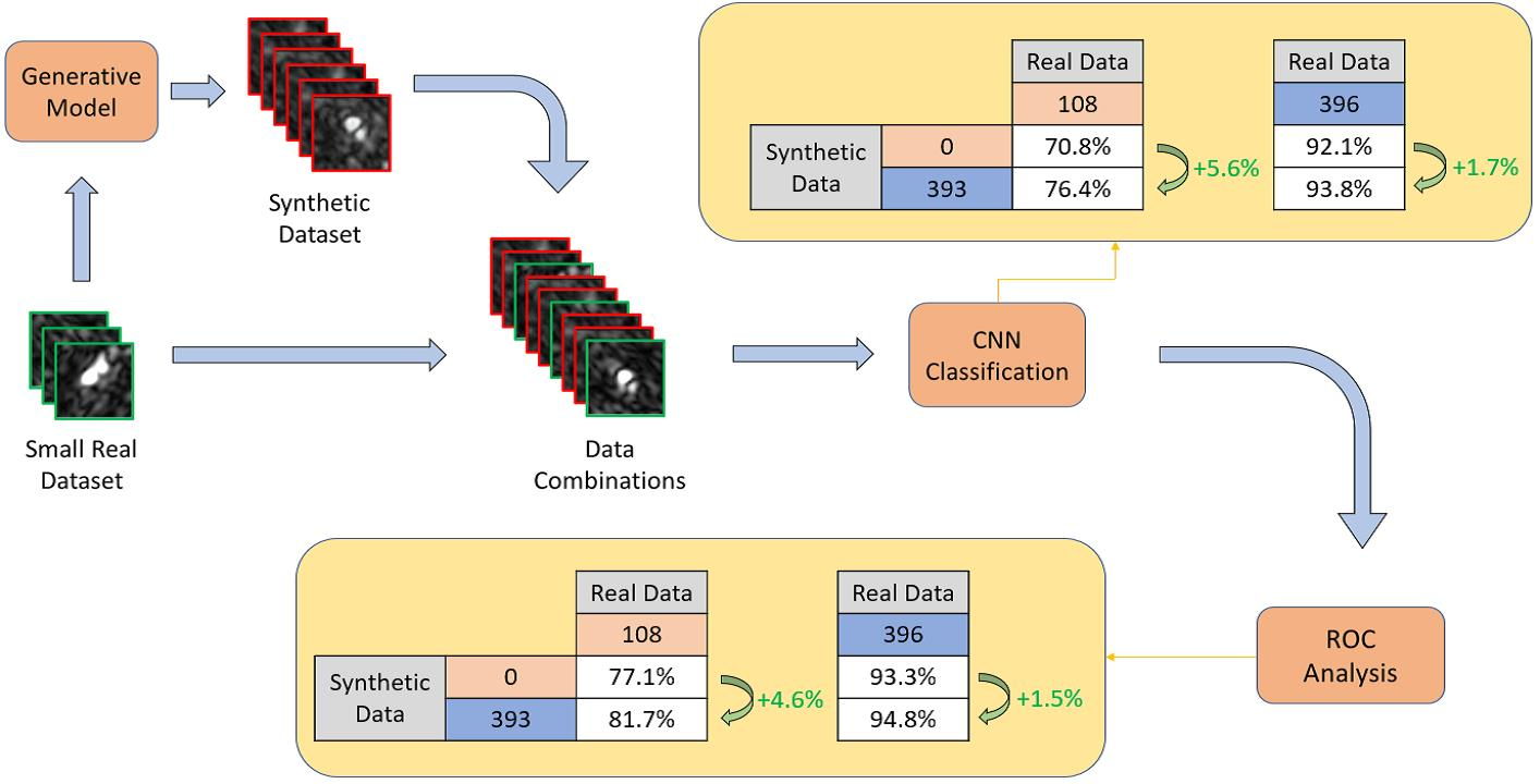
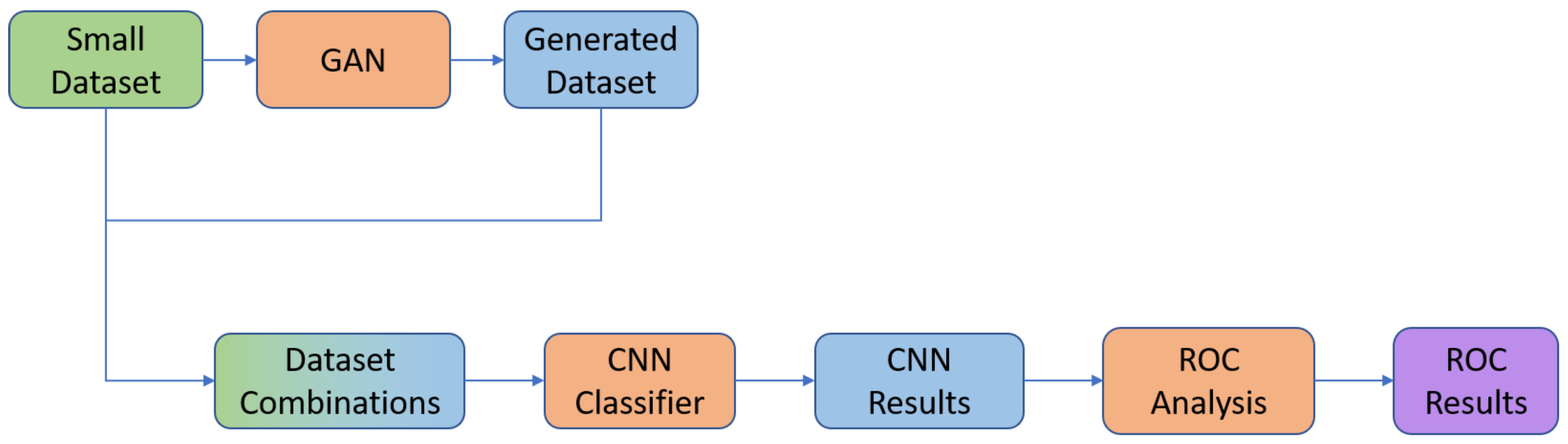
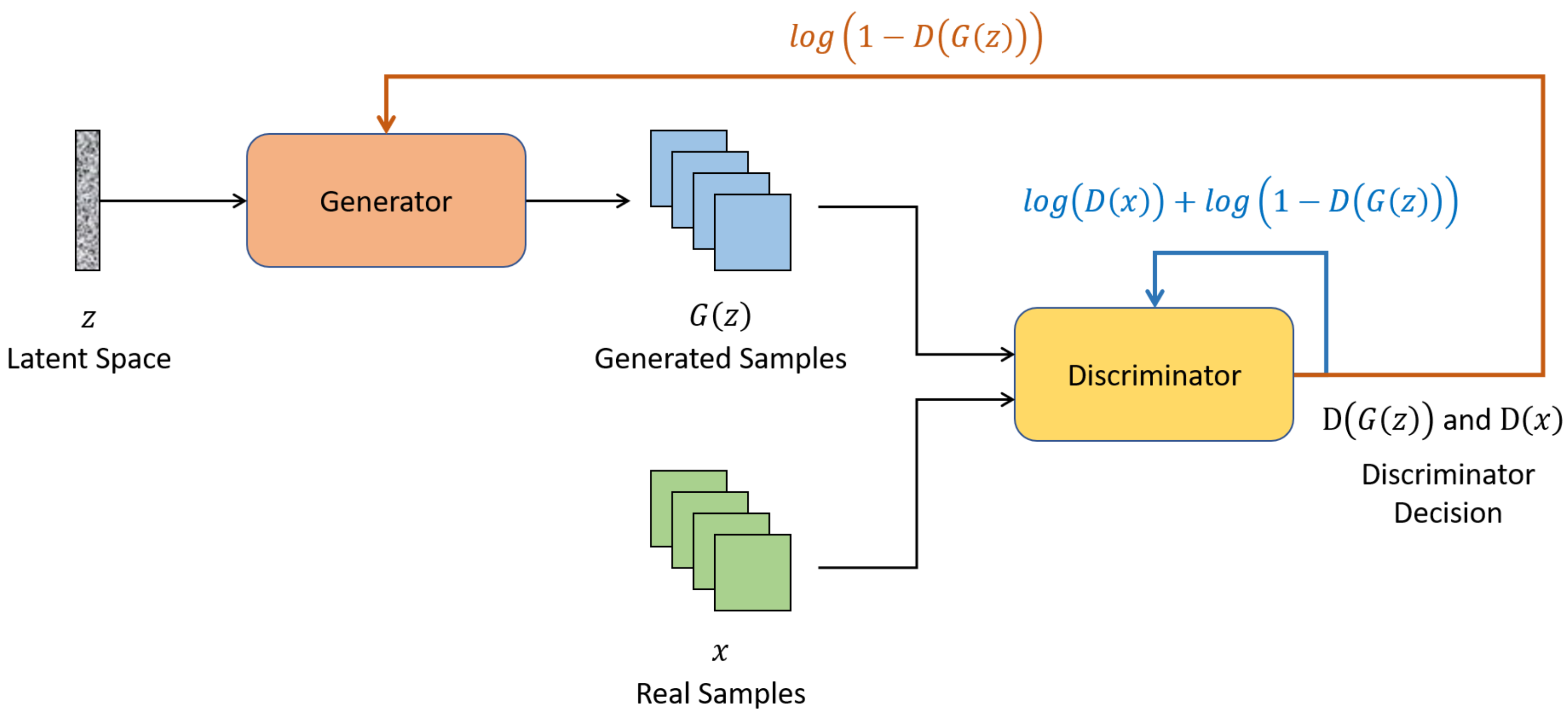
Generative Adversarial Networks (GAN) have also been widely suggested in SAR ATR as at tool to generate synthetic images. In Reference [15], a Multi-Discriminator GAN (MGAN) was proposed for dataset expansion in combination with a CNN classifier. The conducted analysis demonstrated that inclusion of synthetic data in the training can improve the CNN accuracy especially when the number of real images is low. Moreover, in Reference [16], a novel Integrated GANs (I-GAN) model for SAR image generation and recognition was presented combining the ability of the unconditional and conditional GANs for unsupervised feature extraction and supervised image-label matching, respectively. Performance analysis in the MSTAR dataset showed that the proposed framework can generate high quality SAR images outperforming previously proposed semi-supervised learning methods.

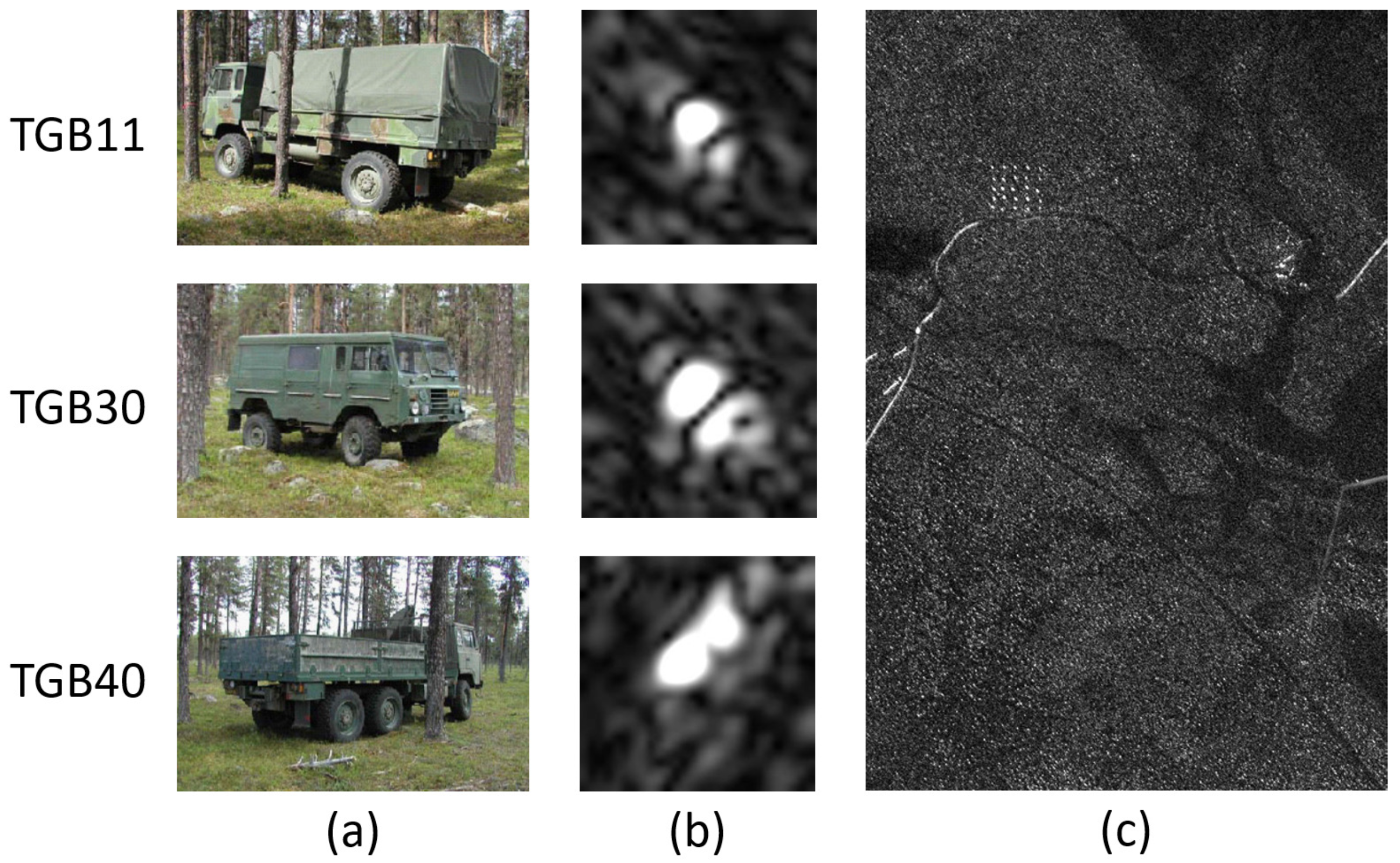
A common limitation of all the above mentioned approaches and of most of the SAR ATR literature is that these are designed and applied on high-resolution SAR images and such a scenario is not always verified. Indeed, the ATR problem becomes even more difficult when the SAR images are not acquired with high spatial resolution due to sensor’s limitations and/or to the actual SAR imaging mode used, such as in Foliage Penetrating (FOPEN) SAR [17]. FOPEN SAR uses relatively low carrier frequencies in order to be able to penetrate canopies, and as a consequence has relatively low bandwidths in both range and cross-range directions, meaning that the final SAR image has a relatively poor spatial resolution, and while such a resolution is enough to detect extended targets, such as vehicles hidden under canopies [18], the target recognition task become very challenging. The problem of low resolution SAR and FOPEN SAR ATR has been only marginally investigated in the literature mainly due to the lack of data availability to the research community. In Reference [2], the performance of SAR ATR was examined using imagery of three different resolutions. Results demonstrated significant impact lowering resolution has on the classification performance, as well as the improvement super-resolution can offer. For these reasons, we are investigating whether the consolidated techniques in the area of AI, such as CNNs and GANs, can be used also in this context to provide a significant operational advantage, such as reducing the need to gather large datasets in hostile environments.

To assess the potential of CNNs and GANs in this context, this paper introduces a framework for target recognition in FOPEN SAR imagery. The framework is applied to the CARABAS II dataset [19] and exploits CNNs in conjunction with GANs to address the ATR challenge of limited data availability by performing an augmentation of the dataset that allows a more reliable training of the CNN. Additionally, the framework introduces an Receiver Operating Characteristic (ROC)-based analysis applied on the CNN output to refine the performance of the recognition framework, while providing an assessment of the confidence that the target recognition framework has when labeling the targets. It is worth noting that aim of this work is not to compare the performance of the proposed framework with existing methods but to demonstrate the capabilities AI can enable in the challenging topic of FOPEN SAR ATR.

The reminder of the paper is organized as follows: Section 2 discusses the proposed Framework, including data generation (Section 2.1), CNN implementation (Section 2.2), ROC Analysis (Section 2.3), and the dataset used (Section 2.4). Section 3 presents the results of the framework, by first presenting the choice of GAN in Section 3.1 with the choice of CNNs described in Section 3.2. The performance analysis is provided in Section 4. Section 5 concludes the paper.

2. Materials and Methods

This section describes the proposed framework for low resolution SAR ATR. The workflow of this framework is illustrated in Figure 1. In order to train a deep learning classifier, a large dataset can greatly increase the classification performance and relative confidence. However, this is not always available, therefore making the application of deep learning not directly suitable to many scenarios. In these cases, augmentation techniques can be used to add small variations to the samples in the dataset, so to present the classifier with a more varied representation of the input data. However, augmentation is a rather simplistic approach. Therefore, in the ATR framework presented in this work, the generation of new data for training is achieved through the use of a Generative Adversarial Network (GAN).

After identifying the GAN most suitable for the specific scenario, the first step is to use the GAN to generate new synthetic samples, which are introduced into the training of a CNN classifier. After training is complete, the classification results are then further refined through a thresholding process, where the optimal threshold is computed with a Receiver Operating Characteristic (ROC) Curve. This additional step allows the classifier to be more confident in its decisions, therefore reducing the number of incorrect classifications.

2.1. Synthetic Data Generation with GANs

Generative adversarial networks (GANs) [20] are a generative modeling method capable of learning deep representations without extensively annotated training data. The basic principle of GANs is in the coexistence of a generator and a discriminator which play against each other in an adversarial process. The generator creates samples which aim to have the same distribution as the training data. The discriminator examines such samples and determines whether they are real or synthetic, and learns through traditional supervised learning methods. The goal of the generator is to create synthetic data that is indistinguishable from the real data, and it must learn to create samples which are drawn from the same distribution as the training data.

Within the original GAN structure [20], both the generator and discriminator are established as multilayer perceptrons. A fixed-length vector is first randomly drawn from a gaussian distribution. The vector is then used as an input to the generator, providing a random seed for the generative process. The vector space—otherwise referred to as latent space—is a projection of a data distribution. With respect to GANs, the generator learns to assert meaning to points in a chosen latent space, such that new points drawn from the latent space can be provided to the generator model as input, and used to generate new and different output examples. Noise is also added in input to the generator, as it allows the GAN to create a wide variety of data, by sampling from different places in the target distributions. The discriminator acts as a classifier, which takes an unknown sample from either the generator or real training data and predicts a binary class label, i.e., real or synthetic.

This training process is described by the value function in Equation (1), where the latent space is represented as z and the discriminator and generator are defined as $D\left(·\right)$ and $G\left(·\right)$, respectively. $\mathbb{E}$ is the expectation operator.

$$\underset{G}{min}\underset{D}{max}V(D,G)={\mathbb{E}}_{x\sim P_{\mathrm{data}}\left(x\right)}[log\left(\mathrm{D}\left(\mathrm{x}\right)\right)]+{\mathbb{E}}_{\mathrm{z}\sim P_z\left(\mathrm{z}\right)}[log(1-D\left(G\left(z\right)\right)].$$

(1)

The typical layout of a GAN architecture is illustrated in Figure 2, where the input to the generator is a random sample from the latent space z. The output $G\left(z\right)$ from the generator is then fed into the discriminator, alongside a sample from the real distribution. The discriminator assigns a value to each of the samples, according to its belief of if the sample is real (1) or synthetic (0). These two outputs are then utilized to analyze the performance of the two models, where the generator is trained to minimize the function $log(1-D(G\left(z\right)\left)\right)$. This, in turn, trains the generator to produce images that the discriminator cannot identify as synthetic (i.e., $D\left(G\right(z\left)\right)\approx 1$). Alongside the training of the generator, the discriminator is trained to maximize the function $log\left(D\right(x\left)\right)+log(1-D(G\left(z\right)\left)\right)$, which in turn aims to train the discriminator to maximize the probability of correctly identifying the real samples, $\left(D\right(x\left)\right)$, whilst also correctly identifying the synthetic samples ($D\left(G\right(z\left)\right)$).

The two models are trained in parallel, therefore introducing a form of competition, where each network tries to outperform the other. The training process is complete when the two networks are no longer able to improve on their current state. That is, the generator is able to produce samples that are indistinguishable from real samples, and the discriminator is no longer able to tell the difference between real and synthetic samples. This is what is known as Nash equilibrium [21]. Once complete, the generator can then be used to generate new, unseen synthetic samples.

Due to the complex training process, GANs are sensitive to instabilities during the training process, and this can lead to two well-document problems, namely gradient vanishing and mode collapse. Gradient vanishing can become an issue when any subset of data distribution and model distribution are disjointed, such that the discriminator identifies real and synthetic data perfectly, which means that the generator no longer improves [21]. Mode collapse occurs when the generator creates the same or similar output, as the model distribution only encapsulates the major or single modes of data distribution to misdirect the discriminator. Traditionally there is a trade-off between image quality and mode collapse, where improvements in image quality cause a lack of image diversity. Variations of the original GAN architecture have been proposed in literature, to overcome the aforementioned two issues. In the context of the work presented here, two GAN alternative architectures have been considered, namely Deep Convolutional GANs (DCGANs) [22] and, Wasserstein GAN + Gradient Penalty (WGAN-GP) [23].

In DCGANs, the generator is made of convolutional-transpose layers, batch norm layers and ReLU activations. DCGANs also use batch normalization for many of the layers in both the discriminator and the generator, with two minibatches for the discriminator normalized separately. The final layer of the generator and first layer of the discriminator are not batch normalized, such that the model can learn the correct mean and scale of the data distribution. This inclusion of batch normalization was shown to reduce the effects of mode collapse, as well as assisting gradient flow [22].

WGAN-GP is a type of GAN which uses the Wasserstein loss formulation [23], plus a gradient norm penalty. This aims to achieve Lipschitz continuity, which is a general solution to make the gradient of the optimal discriminative function reliable, allowing for more stable training of GANs and higher quality generated data [24]. Instead of using a discriminator to classify/predict the probability of generated images being real or synthetic, WGANs uses a critic function which scores the likelyhood of an image of being real or synthetic. The Wasserstein distance is informally defined as the minimum cost of transporting mass in order to transform the distribution q into the distribution p [23]. The critic function has a more stable gradient with respect to its input, therefore making the optimization of the generator easier.

When comparing different GAN models, the lack of an objective loss function during training is an issue. To compare GAN models, different metrics have been proposed in literature. To this aim, the inception score [25] is a widely used metric, which evaluates the quality of the generated data by passing the samples into the Inception v3 [26] classification model, the classification of which then determines the quality of the generated images. This evaluation approach, however, does not actually provide insight into the similarity between real samples and synthetic ones. In fact, this should be the focus of attention when synthetic samples are to be used to enhance datasets for classification applications. Therefore, a metric that measures the similarity between real and synthetic samples should be used, when choosing the best GAN for an application. In this work, the Fréchet Inception Distance (FID) is used, as it compares the statistics of generated and real samples. This is done by measuring the distance between the Inception V3 activation distributions of both cases, i.e., real and synthetic samples. To achieve this, the distributions of an intermediate layer of the inception V3 network are extracted. The means (${\mu }_r,{\mu }_g$) and covariances (${\mathsf{\Sigma }}_r,{\mathsf{\Sigma }}_g$) are then used to evaluate the FID score as,

$$\mathrm{FID}={\left(∥{\mu }_r-{\mu }_g∥\right)}^2+Tr\left({\mathsf{\Sigma }}_r+{\mathsf{\Sigma }}_g-2{\left({\mathsf{\Sigma }}_r{\mathsf{\Sigma }}_g\right)}^{\frac{1}{2}}\right),$$

(2)

where Tr is the trace operator, and the distributions are taken from the 2048-dimensional activation’s of the Inception-v3 pool3 layer [27]. A low FID score indicates more similar distributions, with a FID score of zero representing identical distributions. In this context, the results are reported in Section 3.2, show that, for the data used in this work, the DCGAN generates synthetic images with the lowest FID score.

2.2. Image Classification with CNNs

A convolutional neural network (CNN) is a type of deep neural network often applied to problems involving image data [28], and its architectural design was initially inspired by research on primate’s visual cortex [29]. The key feature of a CNN is that the network learns the weights for its convolutional filters during training, rather than relying on hand-crafted filters that are designed to identify specific features within an image. The filters in the initial convolutional layers may be used to identify simple features, such as straight lines, with subsequent convolutional layers being used to identify more complicated features composed of combinations of lower-level features. For the convolutional filters, the aim is to learn sets of weights that extract features from the input which prove useful for correctly classifying the input data, thus minimizing the loss for the specific task under consideration.

In the framework presented in this work, CNNs are used to classify real low resolution SAR images, with and without the use of synthetic images generated with a GAN network as described in the previous section in the training set. In order to provide a thorough investigation of the effects of different mixes of real and synthetic samples on the classification accuracy of the CNN under exam, multiple network architectures are tested. This analysis allows for any bias of a single network to be mitigated. The CNNs evaluated in this work are Resnet18 [30], Alexnet [31], Vgg11 [32], Squeezenet [33], Densenet121 [34], and Inceptionv3 [26], and they have been selected for testing as they all achieve high classification accuracy on the ImageNet dataset.

To train a classifier, the data must be first split into training and test data. This allows the networks ability to classify unseen data to be evaluated. In this framework, all the test data is compiled using real samples. Once the data is prepared, the networks can then be trained. In this case, transfer learning is used to speed up the training process. The technique of transfer learning makes use of a pre-trained network which is able to reduce an input image into a high dimensional feature space. This feature space is then transformed into a classification with fully connected layers. It is these layers that are re trained in transfer learning. This speeds up the training process and also removes the need of an extremely large dataset for training the full network.

2.3. ROC Analysis for Error Rejection

In the final step of the proposed framework, the Receiver Operating Characteristic (ROC) Curve is used to evaluate a confidence threshold to the CNN classification output. In this way, only classification labels which bear an acceptable level of confidence are retained, while low confidence outputs are rejected (i.e., labeled as unknown). For each class, a separate optimal confidence threshold is computed as follows.

Each class has N associated test samples, with $N^c$ correctly classified samples, and $N^e$ incorrectly classified samples, so that $N=N^c+N^e$. Each classification label in output has a confidence $p_n$ with $n=[1,N]$. Given any value of threshold $\tau$, if it is $p_n<\tau$, then the n-th classification, i.e., test sample, is rejected; if it is $p_n\ge \tau$, the n-th classification is retained. Of all the classifications retained for a given value of $\tau$, $N_{\tau }^e$ is the number of incorrect classifications retained after thresholding, while $N_{\tau }^c$ is the number of correct classifications retained. The coordinates ${\mathbf{x}}_{\tau }=(N_{\tau }^e/N^e,N_{\tau }^c/N^c)$ identify points on the ROC curve, in a graph where the x-axis is normalized between 0 and 1, and it represents the error rate after thresholding, while the y-axis represents the correct classification rate, and it is also normalized between 0 and 1. In such an ROC curve, each point has an associated value of threshold $\tau$, and the optimal operating point corresponds to the top left point on the curve, as this simultaneously minimizes the error rate and maximizes the correct classification rate. Ideally, the ROC curve can be written as:

$$N_{\tau }^c/N^c=f\left(N_{\tau }^e/N^e\right).$$

(3)

Therefore, the optimal threshold ${\tau }^{opt}$ for the class can be found as:

$${\tau }^{opt}=\underset{\tau }{argmin}\left\{\underset{N_{\tau }^e/N^e}{argmax}\left\{f\left(N_{\tau }^e/N^e\right)-N_{\tau }^e/N^e\right\}\right\}.$$

(4)

In the proposed framework, this ROC analysis is applied to each classification individually, therefore providing as many thresholds as the number of classes to be discriminated. Once each threshold is found, the results are then re-evaluated. If a classification is below the given threshold, the associated test sample is discarded. This process, in turn, then reduces the number of errors made by the classifier. As well as a new classification accuracy, the ROC analysis also produces a rejection rate metric. This is a percentage of the input samples that the network has classified with low confidence. Lower rejection rates mean that the overall framework is more reliable as the classifier is more confident in its output.

2.4. Dataset Description

The data used in this framework was a publicly available dataset of 24 magnitude CARABAS-II VHF-Band SAR images. These images were obtained during a flight campaign held in Sweden in 2002 [35]. The system transmits HH-polarized radio waves between 20 and 90 MHz, corresponding to wavelengths between 3.3 and 15 m. In the imaged areas, 25 military vehicles are concealed by the forest, in four deployments (for reader’s convenience, see Reference [35]). The motivation for the campaign was to collect new low VHF-band SAR images of targets under foliage canopies, which would then be utilized for new object detection algorithms [18]. The targets deployed during the measurement campaign were three terrain vehicles of differing size: the TGB11, TGB30, and TGB40 shown in Figure 3a. In total, seventeen missions were carried out, each performed under different operating conditions. The variables in consideration for each missions were the incidence angle, flight heading, target orientation, target size, and radio Frequency Interference (RFI) (For more information regarding the flight missions, the reader is referred to Reference [35].). Of the seventeen missions, four have been made available to the public, named Sigismund, Karl, Frederik, and Adolf-Frederik. The operating conditions for these missions are shown in

Table 1. Mission configurations of CARABAS-II VHF-Band SAR dataset.

Target Deployment	Flight Heading (deg)	Incidence Angle (deg)	RFI	Target Heading (deg)
Sigismund	225	58	High	225
Sigismund	135	58	Low	225
Sigismund	230	58	High	225
Karl	225	58	High	315
Karl	135	58	Low	315
Karl	230	58	High	315
Frederik	225	58	High	225
Frederik	135	58	Low	225
Frederik	230	58	High	225
Adolf-Fredrik	225	58	High	270
Adolf-Fredrik	135	58	Low	270
Adolf-Fredrik	230	58	High	270

, where two images were captured for each condition, providing a total of 24 images. Each image contained ten TGB11s, eight TGB30s, and seven TGB40s.

Figure 3c shows an example SAR image, as well as examples of the extracted targets (Figure 3b). These are extracted as 38 × 38 images with the use of the provided ground truth positions of each target within the images.

In order to ensure a fair distribution of the three targets, the same count of each was used during training. To accommodate for the low representation of the TGB40 class (14 per configuration), any additional samples of the remaining classes were discarded, such that the sample count of each class was equal. This provided a total of 168 samples of each target class, and a total dataset size of 504.

Additionally, each mission configuration was equally represented in both training and testing, the train/test ratio was chosen such that the fourteen samples per mission configuration were split equally. It was decided that a split of 11 training samples and 3 test samples would provide a suitable train/test ratio, providing a train dataset of 396 samples and a test dataset of 108. This was to be used as the base dataset, that synthetic data could be introduced into, to form eight separate data configurations, detailed in Section 3.1.

3. Results

3.1. GAN Selection

When identifying the optimal GAN architecture, all of the real data was utilized to gain a full understanding of the performances. Once trained, the individual FID scores were evaluated and are presented in

Table 2. Fréchet Inception Distance Scores of each GAN.

GAN Model	FID Score
GAN	310.2
DCGAN	163.42
WGAN-GP	171.12

. DCGAN provided the lowest FID score, indicating that it was best able to emulate the training data. This is reflected also in the appearance of the generated images, as an example some of the TGB11 GANs outputs are shown in Figure 4.

The original GAN architecture generates images that are noiser and more blurred. DCGAN and WPGAN-GP produce images of similar quality; however, it can be seen that the DCGAN produces sharper samples when compared with WPGAN-GP. This agrees with the FID scores, and DCGAN was, therefore, the chosen model for this framework.

Using the DCGAN architecture, 393 synthetic samples were generated (131 of each target type). These were then introduced with the real samples to form the assessment configurations (C1 to C8). These can be seen in

Table 3. Definition of the real/synthetic sample split in each configuration.

	Training Data			Testing Data
Configurations	Real	Synthetic	Total	Real
C1	396	0	396	108
C2	396	132	528	108
C3	396	261	657	108
C4	396	393	789	108
C5	252	0	252	108
C6	252	393	645	108
C7	108	0	108	108
C8	108	393	501	108

, where configurations C1-C4 analyze the effect of introducing additional synthetic samples into the training process, while the pairs of configurations C1/C4, C5/C6, and C7/C8 assess the effect of the integration of synthetic data on configurations with much more limited real data availability.

3.2. CNN Selection

Classification of the ImageNet dataset [36] is a well known deep learning challenge. For years, improvements have been made, ever increasing the resulting scores, to the point that deep learning architectures are able to outperform a human. The CNN architectures used in this comparison have provided great improvements in the field of classification and have performed well on the ImageNet dataset in the past. To test the validity of these architectures, an initial test was performed using C1 from Table 3. For each of the networks, the settings were chosen as shown in

Table 4. Hyperparameters for training the Convolutional Neural Networks (CNNs).

Optimizer	Adam
Learning Rate	0.001
Batch Size	32
Epochs	100

and the results are shown in

Table 5. Initial CNN architecture test results, trained on C1.

Network	Test Accuracy
Resnet18	90%
Alexnet	34%
Vgg11	94%
Squeezenet	36%
Densenet121	87%
Inceptionv3	83%

.

It can be seen that the Alexnet and Squeezenet architectures were not able to provide comparable results when trained with the data available. Therefore, these networks were no longer considered for this framework.

As well as this initial test with dataset C1, traditional image augmentation techniques were also tested. This consists of expanding the available dataset by applying various augmentations, such ad rotations and reflections. This technique can be considered as another approach to improve the performance of classification when using a limited dataset. However, when tested with the data samples in question, the accuracy performance was found to decrease.

3.3. Testing with GAN Images

The four networks were trained on each of the 8 configurations. In order to mitigate potential biases in performance each configuration is randomly represented four times (C1_1, C1_2, C1_3, C1_4, etc.).

Table 6. Original classification accuracy of each CNN on each of the configurations.

	Networks
Configuration	Densenet	Inception	Resnet	Vgg
C1	87.5%	87%	93.1%	92.1%
C2	90%	89.8%	93.3%	92.8%
C3	91.4%	88.7%	93.3%	91.9%
C4	92.6%	91%	93.1%	93.8%
C5	79.4%	81.3%	83.3%	83.8%
C6	87.3%	84%	86.1%	90.5%
C7	61.1%	65.5%	68.3%	70.8%
C8	71.3%	71.5%	78%	76.4%
Average	82.6%	82.3%	86.1%	86.5%

provides the obtained target recognition results, where the presented value is the average over the four configuration iterations.

A final investigation consisted of assessing the performance of the trained networks in cases where noise is present within the test samples. This was to identify the robustness of the trained network to the presence of multiplicative noise, where multiplicative noise is most common in the case of SAR imagery. In this case, the modulus of each pixel is multiplied with the square root of a Gamma random variable [8]. For the results presented, values of the shape parameter $\nu$ of the Gamma distribution used are of 0.5 and 10, and the scale parameter $\mathsf{\mu }=1/\nu$. These were applied to each of the dataset configurations in Table 3, and the resulting performance of the VGG architecture is given in

Table 7. Accuracy of the Vgg on each dataset configuration corrupted by various levels of multiplicative noise.

Configuration	No Noise	$\mathit{\nu }=10$	$\mathit{\nu }=0.5$
C1	92.1%	88.9%	63.7%
C2	92.8%	89.6%	61.6%
C3	91.9%	87.7%	64.6%
C4	93.8%	88.7%	60.4%
C5	83.8%	78.9%	50.2%
C6	90.5%	86.1%	56.3%
C7	70.8%	63.4%	51.2%
C8	76.4%	71.3%	50.5%

.

3.4. ROC Analysis

As the final step of the proposed framework, ROC analysis was applied to the confidence levels of each network. An example ROC curve for the TGB30 target from the Densenet121 architecture trained on C1 is shown in Figure 5. The best threshold is found by subtracting the ROC curve (blue) from the ROC space diagonal (red), and then selecting the highest point on the resulting plot (green). This process allows the best threshold for each classification to be found, which aims to keep the correct classification rate high, whilst also reducing the error rate. Once the best threshold for each target for each network is found, the confidence of each network is reevaluated. If the confidence is lower than the set threshold, the sample is discarded. This analysis, therefore, provides two seperate metrics, a new classification accuracy and a rejection rate. An ideal threshold would aim to increase the new accuracy whilst keeping the rejection rate low. The new accuracies after the ROC analysis stage is shown in

Table 8. Classification accuracy after ROC analysis.

	Networks
Configuration	Densenet	Inception	Resnet	Vgg
C1	95.8%	94.4%	98.5%	93.3%
C2	95.9%	97.2%	97.3%	93.2%
C3	95.8%	96%	96.7%	95.4%
C4	97.2%	96.4%	99.1%	94.8%
C5	89.6%	92.2%	95.7%	88%
C6	94%	93.1%	93.6%	94.9%
C7	71.5%	74.4%	80.2%	77.1%
C8	81%	87%	87.3%	81.7%
Average	90.1%	91.3%	93.5%	89.8%

, and the corresponding rejection rates are provided in

Table 9. Rejection rate after ROC analysis.

	Networks
Configuration	Densenet	Inception	Resnet	Vgg
C1	44.4%	38%	25%	7.4%
C2	31.5%	34.5%	23.1%	4.4%
C3	27.8%	35.6%	22.5%	14.1%
C4	25.9%	21.8%	25.9%	6.7%
C5	41.9%	37.7%	46.5%	16.9%
C6	34.3%	46.1%	35.2%	14.1%
C7	52.1%	45.8%	56.7%	30.3%
C8	50%	57.4%	45.1%	24.1%

.

4. Discussion

4.1. Testing with GAN Images

The highest original test accuracy was achieved by Vgg on C4 (93.8%), as seen in Table 6. This was a configuration that included the maximum amount of synthetic samples. However, this does not necessarily indicate that the inclusion of synthetic samples provides a significant improvement as, when compared to the Resnet results, it can be seen that without any synthetic data, an accuracy of 93% can be achieved. To better visualize these results, Figure 6 shows how the accuracy of each network varies over different counts of synthetic data. These results correspond to configurations C1, C2, C3, and C4 in Table 3.

From this graph, it can be seen that for the selected scenario, introducing additional synthetic samples introduces a limited performance increase. The Resnet18 and Vgg11 architectures see very little improvement over the range of synthetic data, where Densenet121 and Inceptionv3 show a better response. However, even in the best case, only an accuracy increase of 5% is achieved.

In particular, Resnet only varies by 0.2%, Densenet increases from 87.5% to 92.6%, and VGG has a maximum of 93.8% when 393 synthetic data are used, while Inception increases from 87% to 91%.

Another insight that can be gained from the results is to see how the accuracy changes when the availability of real samples is reduced. These results correspond to the configuration pairings C1/C4, C5/C6, and C7/C8 in Table 3 and can be seen in Figure 7. This shows that the introduction of synthetic samples can greatly aid the training process when a small amount of real samples are available (This is a very important aspect as it is difficult and expensive to gather large training dataset in the investigated application domain.). It can be seen that as less real samples become available, the potential benefit of additional synthetic data increases. This can especially be seen in the case of Resnet18, where the potential gain in accuracy increases 0% to 9.7%, therefore showing that the the use of synthetic samples becomes more important in poorly represented datasets.

The difference for Densenet increases from 5.1% to 10.2% with decreasing number of real data samples used, similarly for Resnet, the performance improvement moves from 0.2% to 9.7% with this trend not confirmed only for the case of the Vgg11 network.

The response of the VGG network to noisy samples can also be analyzed. The results of the multiplicative noise experiment can be seen in Figure 8. These results show that, when light noise is present ($\nu =10$), a similar trend in the results are exhibited, being that the inclusion of synthetic data is able to boost performance when limited real data is available. However, it can be seen that, when severe noise is present ($\nu =0.5$), the accuracy of the network is greatly reduced, with little suport from the additional synthetic samples. This is as to be expected, as this level of severe noise is able to remove any useful information from within the samples.

4.2. ROC Analysis

As with the results in Section 4.1, it is best to analyze the response of the networks first as a function of synthetic data (C1, C2, C3, C4), shown in Figure 9, where both the network accuracy and rejection rates are shown. These plots show that, after ROC analysis, the accuracy over the differing levels of synthetic data follows the same pattern as seen in Section 4.1 (Figure 6), where, due to the abundant presence of real data, the addition of synthetic data is unable to provide significant improvements.

The best decrease in reject rate is for Densenet, where it decreases from 44% to 25.9%. All the other classifiers maintain approximately constant performance as more synthetic data is added. Inception has a big loss in performance at the end from 35% to 21.7%, while it is worth noting that Vgg already produces a low rejection rate and does not benefit much when synthetic data are introduced.

Figure 10 shows the response of the networks as the availability of real data is altered (C1, C4, C5, C6, C7 & C8). This also agrees with the results found in Section 4.1 (Figure 7) where, in the case of when real data is sparse, the accuracy can be increased by introducing additional synthetic data. This plot also provides new analysis, in which it can be seen that the inclusion of synthetic data also increases the confidence level of each network. With the exception of inceptionv3, the additional synthetic data increases the confidence of the networks, independently from the amount of real data present in the training set. The maximum increase of 18% is obtained in the case of Densenet, when the maximum amount of real data was available. This shows that the additional synthetic data can increase the overall confidence of the classifications.

In particular, from Figure 10 it can be observed that with the exception of Inception, the inclusion of 396 synthetic samples always reduces the rejection rate, as well as increasing the accuracy. The best examples are Densenet and Vgg, where the difference in reject rate for Densenet increases from 2% to 18%. The accuracy difference decreased. For inception, the inclusion of synthetic data only comes into effect when there is a relatively large number of real data, providing a decrease in rejection rate from 46% to 21.7%, even though the accuracy does increase with the synthetic data.

5. Conclusions

In this paper, a framework to perform SAR-based ATR in low resolution Foliage Penetrating SAR images is proposed. This specific ATR challenge is particularly difficult given the low resolution nature of the data and the fact that is difficult to obtain well populated datasets. The proposed approach investigates the potential use of CNN and GANs to address the target recognition problem. The paper has analyzed four different architectures of CNNs and how the introduction of GANs derived training data could benefit the capability of an ATR system to correctly recognize targets hiding under canopies. The analysis on the accuracy of the four networks and how they perform when trained with different amounts of real data and synthetic data has confirmed that the introduction of GANs generated data can improve the ATR performance, with larger benefits achieved when real training data are more limited. This trend has been confirmed also when assessing the confidence of a specific network to perform the recognition task, with rejection rates generally decreasing with increasing synthetic data injected at the training stage. Future work will investigate the use of ad-hoc networks to address this task, as well as the introduction of additional of the use of Single Look Complex SAR images and Polarimetric information.

References

1. Novak, L.M.; Halversen, S.D.; Owirka, G.J.; Hiett, M. Effects of Polarization and Resolution on SAR ATR. IEEE Trans. Aerosp. Electron. Syst. 1997, 33, 102–116. [Google Scholar] [CrossRef]
2. Novak, L.; Owirka, G.; Weaver, A. Automatic target recognition using enhanced resolution SAR data. IEEE Trans. Aerosp. Electron. Syst. 1999, 35, 157–175. [Google Scholar] [CrossRef]
3. Kechagias-Stamatis, O.; Aouf, N. Automatic Target Recognition on Synthetic Aperture Radar Imagery: A Survey. arXiv 2020, arXiv:cs.CV/2007.02106. [Google Scholar]
4. El-Darymli, K.; Gill, E.W.; Mcguire, P.; Power, D.; Moloney, C. Automatic Target Recognition in Synthetic Aperture Radar Imagery: A State-of-the-Art Review. IEEE Access 2016, 4, 6014–6058. [Google Scholar] [CrossRef] [Green Version]
5. Zhao, Q.; Principe, J.C. Support vector machines for SAR automatic target recognition. IEEE Trans. Aerosp. Electron. Syst. 2001, 37, 37. [Google Scholar] [CrossRef] [Green Version]
6. Doo, S.H.; Smith, G.; Baker, C. Reliable target feature extraction and classification using potential target information. In Proceedings of the 2015 IEEE Radar Conference (RadarCon), Arlington, VA, USA, 10–15 May 2015; pp. 0628–0633. [Google Scholar]
7. Srinivas, U.; Monga, V.; Raj, R. SAR Automatic Target Recognition Using Discriminative Graphical Models. IEEE Trans. Aerosp. Electron. Syst. 2014, 50, 591–606. [Google Scholar] [CrossRef]
8. Clemente, C.; Pallotta, L.; Gaglione, D.; De Maio, A.; Soraghan, J.J. Automatic Target Recognition of Military Vehicles with Krawtchouk Moments. IEEE Trans. Aerosp. Electron. Syst. 2017, 53, 493–500. [Google Scholar] [CrossRef] [Green Version]
9. Blasch, E.; Majumder, U.; Zelnio, E.; Velten, V. Review of recent advances in AI/ML using the MSTAR data. In Algorithms for Synthetic Aperture Radar Imagery XXVII; Zelnio, E., Garber, F.D., Eds.; International Society for Optics and Photonics, SPIE: Bellingham, WA, USA, 2020; Volume 11393, pp. 53–63. [Google Scholar]
10. Chen, S.; Wang, H.; Xu, F.; Jin, Y. Target Classification Using the Deep Convolutional Networks for SAR Images. IEEE Trans. Geosci. Remote Sens. 2016, 54, 4806–4817. [Google Scholar] [CrossRef]
11. Zhang, X.; Qin, J.; Li, G. SAR target classification using Bayesian compressive sensing with scattering centers features. Prog. Electromagn. Res. 2013, 136, 385–407. [Google Scholar] [CrossRef] [Green Version]
12. Zhang, F.; Liu, Y.; Zhou, Y.; Yin, Q.; Li, H.C. A lossless lightweight CNN design for SAR target recognition. Remote Sens. Lett. 2020, 11, 485–494. [Google Scholar] [CrossRef]
13. Huang, X.; Yang, Q.; Qiao, H. Lightweight Two-Stream Convolutional Neural Network for SAR Target Recognition. IEEE Geosci. Remote Sens. Lett. 2020, 1–5. [Google Scholar] [CrossRef]
14. Zhang, F.; Hu, C.; Yin, Q.; Li, W.; Li, H.; Hong, W. Multi-Aspect-Aware Bidirectional LSTM Networks for Synthetic Aperture Radar Target Recognition. IEEE Access 2017, 5, 26880–26891. [Google Scholar] [CrossRef]
15. Zheng, C.; Jiang, X.; Liu, X. Semi-Supervised SAR ATR via Multi-Discriminator Generative Adversarial Network. IEEE Sens. J. 2019, 19, 7525–7533. [Google Scholar] [CrossRef]
16. Gao, F.; Liu, Q.; Sun, J.; Hussain, A.; Zhou, H. Integrated GANs: Semi-Supervised SAR Target Recognition. IEEE Access 2019, 7, 113999–114013. [Google Scholar] [CrossRef]
17. Hellsten, H.; Ulander, L.M.; Gustavsson, A.; Larsson, B. Development of vhf carabas ii sar. In Radar Sensor Technology; International Society for Optics and Photonics: Bellingham, WA, USA, 1996; Volume 2747, pp. 48–60. [Google Scholar]
18. Izzo, A.; Liguori, M.; Clemente, C.; Galdi, C.; Bisceglie, M.D.; Soraghan, J.J. Multimodel CFAR Detection in Foliage Penetrating SAR Images. IEEE Trans. Aerosp. Electron. Syst. 2017, 53, 1769–1780. [Google Scholar] [CrossRef] [Green Version]
19. SDMS. Sensor Data Management System Public Web Site. 2018. Available online: https://www.sdms.afrl.af.mil/index.php (accessed on 18 December 2020).
20. Goodfellow, I.; Pouget-Abadie, J.; Mirza, M.; Xu, B.; Warde-Farley, D.; Ozair, S.; Courville, A.; Bengio, Y. Generative Adversarial Nets. In Advances in Neural Information Processing Systems 27; Curran Associates, Inc.: Red Hook, NY, USA, 2014; pp. 2672–2680. [Google Scholar]
21. Bang, D.; Shim, H. Improved training of generative adversarial networks using representative features. arXiv 2018, arXiv:1801.09195. [Google Scholar]
22. Radford, A.; Metz, L.; Chintala, S. Unsupervised representation learning with deep convolutional generative adversarial networks. arXiv 2015, arXiv:1511.06434. [Google Scholar]
23. Gulrajani, I.; Ahmed, F.; Arjovsky, M.; Dumoulin, V.; Courville, A.C. Improved training of wasserstein gans. Adv. Neural Inf. Process. Syst. 2017, 30, 5767–5777. [Google Scholar]
24. Zhou, Z.; Song, Y.; Yu, L.; Wang, H.; Liang, J.; Zhang, W.; Zhang, Z.; Yu, Y. Understanding the Effectiveness of Lipschitz-Continuity in Generative Adversarial Nets. arXiv 2018, arXiv:1807.00751. [Google Scholar]
25. Salimans, T.; Goodfellow, I.; Zaremba, W.; Cheung, V.; Radford, A.; Chen, X. Improved techniques for training gans. Adv. Neural Inf. Process. Syst. 2016, 29, 2234–2242. [Google Scholar]
26. Szegedy, C.; Vanhoucke, V.; Ioffe, S.; Shlens, J.; Wojna, Z. Rethinking the inception architecture for computer vision. In Proceedings of the IEEE Conference on Computer Vision and Pattern Recognition, Las Vegas, NV, USA, 26 June–1 July 2016; pp. 2818–2826. [Google Scholar]
27. Heusel, M.; Ramsauer, H.; Unterthiner, T.; Nessler, B.; Hochreiter, S. Gans trained by a two time-scale update rule converge to a local nash equilibrium. Adv. Neural Inf. Process. Syst. 2017, 30, 6626–6637. [Google Scholar]
28. LeCun, Y.; Boser, B.; Denker, J.S.; Henderson, D.; Howard, R.E.; Hubbard, W.; Jackel, L.D. Backpropagation applied to handwritten zip code recognition. Neural Comput. 1989, 1, 541–551. [Google Scholar] [CrossRef]
29. Hubel, D.H.; Wiesel, T.N. Receptive fields, binocular interaction and functional architecture in the cat’s visual cortex. J. Physiol. 1962, 160, 106. [Google Scholar] [CrossRef]
30. He, K.; Zhang, X.; Ren, S.; Sun, J. Deep residual learning for image recognition. In Proceedings of the IEEE Conference on Computer Vision and Pattern Recognition, Las Vegas, NV, USA, 26 June–1 July 2016; pp. 770–778. [Google Scholar]
31. Krizhevsky, A.; Sutskever, I.; Hinton, G.E. Imagenet classification with deep convolutional neural networks. Commun. ACM 2017, 60, 84–90. [Google Scholar] [CrossRef]
32. Simonyan, K.; Zisserman, A. Very deep convolutional networks for large-scale image recognition. arXiv 2014, arXiv:1409.1556. [Google Scholar]
33. Iandola, F.N.; Han, S.; Moskewicz, M.W.; Ashraf, K.; Dally, W.J.; Keutzer, K. SqueezeNet: AlexNet-level accuracy with 50× fewer parameters and <0.5 MB model size. arXiv 2016, arXiv:1602.07360. [Google Scholar]
34. Huang, G.; Liu, Z.; Weinberger, K.Q. Densely Connected Convolutional Networks. In Proceedings of the CVPR 2017, Honolulu, HI, USA, 21–26 July 2017. [Google Scholar]
35. Lundberg, M.; Ulander, L.M.; Pierson, W.E.; Gustavsson, A. A challenge problem for detection of targets in foliage. In Algorithms for Synthetic Aperture Radar Imagery XIII; International Society for Optics and Photonics: Bellingham, WA, USA, 2006; Volume 6237, p. 62370K. [Google Scholar]
36. Deng, J.; Dong, W.; Socher, R.; Li, L.J.; Li, K.; Fei-Fei, L. Imagenet: A large-scale hierarchical image database. In Proceedings of the 2009 IEEE Conference on Computer Vision and Pattern Recognition, Ieee, Miami, FL, USA, 20–25 June 2009; pp. 248–255. [Google Scholar]
Figure 1. Proposed Automatic Target Recognition (ATR) framework.
Remotesensing 13 00596 g001
Figure 2. Typical Generative Adversarial Networks (GAN) architecture.
Remotesensing 13 00596 g002
Figure 3. (a) Terrain vehicle targets [35] (b) Extracted Synthetic Aperture Radar (SAR) targets (c) Example image from the CARABAS-II VHF-Band SAR dataset.
Remotesensing 13 00596 g003
Figure 4. Generated images from the GANs under review. Classification TGB11.
Remotesensing 13 00596 g004
Figure 5. Resulting ROC Curve for the TGB30 classification from the Densenet121 architecture trained on C1.
Remotesensing 13 00596 g005
Figure 6. Accuracy of each network when altering the count of synthetic data within the training process. These results correspond to configurations C1, C2, C3, and C4.
Remotesensing 13 00596 g006
Figure 7. Accuracy of each network when altering the count of real data within the training process. Two counts of synthetic data are shown. These results correspond to the configuration pairings C1/C4, C5/C6, and C7/C8.
Remotesensing 13 00596 g007
Figure 8. Resulting accuracy of the Vgg architecture when presented with samples corrupted by multiplicative noise. N C represents the count of synthetic data used in training.
Remotesensing 13 00596 g008
Figure 9. Response of networks after ROC analysis with increasing levels of synthetic data.These results correspond to configurations C1, C2, C3, and C4. The orange lines represent the rejection rates of the networks, whilst the blue lines represents the accuracy after ROC analysis.
Remotesensing 13 00596 g009
Figure 10. Response of networks after ROC analysis with increasing levels of real data. These results correspond to the configuration pairings C1/C4, C5/C6, and C7/C8.
Remotesensing 13 00596 g010