
Visual Growth Tracking for Automated Leaf Stage Monitoring Based on Image Sequence Analysis

1
Department of Computer Science and Engineering, University of Nebraska-Lincoln, Lincoln, NE 68588, USA
2
School of Natural Resources, University of Nebraska-Lincoln, Lincoln, NE 68583, USA
3
Agricultural Research Division, University of Nebraska-Lincoln, Lincoln, NE 68583, USA
*
Author to whom correspondence should be addressed.
†
These authors contributed equally to this work.
Remote Sens. 2021, 13(5), 961; https://0-doi-org.brum.beds.ac.uk/10.3390/rs13050961
Submission received: 21 January 2021
/
Revised: 19 February 2021
/
Accepted: 24 February 2021
/
Published: 4 March 2021
(This article belongs to the Special Issue Acquire and Perceive: Novel Approaches for Imaging-Based Plant Phenotyping)
Abstract
:In this paper, we define a new problem domain, called visual growth tracking, to track different parts of an object that grow non-uniformly over space and time for application in image-based plant phenotyping. The paper introduces a novel method to reliably detect and track individual leaves of a maize plant based on a graph theoretic approach for automated leaf stage monitoring. The method has four phases: optimal view selection, plant architecture determination, leaf tracking, and generation of a leaf status report. The method accepts an image sequence of a plant as the input and automatically generates a leaf status report containing the phenotypes, which are crucial in the understanding of a plant’s growth, i.e., the emergence timing of each leaf, total number of leaves present at any time, the day on which a particular leaf ceased to grow, and the length and relative growth rate of individual leaves. Based on experimental study, three types of leaf intersections are identified, i.e., tip-contact, tangential-contact, and crossover, which pose challenges to accurate leaf tracking in the late vegetative stage. Thus, we introduce a novel curve tracing approach based on an angular consistency check to address the challenges due to intersecting leaves for improved performance. The proposed method shows high accuracy in detecting leaves and tracking them through the vegetative stages of maize plants based on experimental evaluation on a publicly available benchmark dataset.
1. Introduction
Visual tracking is an emerging research field that deals with the problem of localizing a pre-specified object in a video sequence. It is a challenging problem with many practical applications, e.g., player detection and tracking in sports videos [1], tracking of pedestrians in video sequences for visual surveillance and scene awareness [2], and moving vehicle detection and tracking for traffic surveillance [3,4]. More recently, tracking has been applied in a completely different domain, i.e., image-based plant phenotyping analysis, for leaf growth monitoring of Arabidopsis [5]. Different plants exhibit different architectures, the complexity of which gradually increases with time. This results in automated growth monitoring of a plant being challenging, as a whole and its parts (e.g., leaves, flowers, roots), based on image sequence analysis. Hence, this research area requires focused and long-term attention from the computer vision community. The role of plants is critical in the context of food security and the wellbeing of humans and animals. The application of visual tracking in automated growth stage determination of economically important crops, e.g., maize and sorghum, for plant phenotyping is yet to be explored despite their role as the source of staple foods in most areas of the world.
Image-based plant phenotyping facilitates the extraction of advanced biophysical traits by analyzing a large number of plants non-destructively in a short period of time with limited manual intervention. Understanding genetic diversity and the impacts of abiotic and biotic stresses on plant performance and yield is of critical importance to address current and emerging issues related to food security and climate variability. For example, in maize, the vegetative growth stage, which is important for yield predictions, is determined by the number of leaves emerging before flowering. Maize is one of three grain crops along with rice and wheat that directly or indirectly provides half of the total world’s calorie consumption each year. Hence, the study of its growth stages influenced by various stress conditions, e.g., drought, salinity, and heat, is of critical importance [6,7]. However, after the natural senescence of the lower leaves, the growth stage determination requires manual splitting of the lower part of the stalk to inspect the internode elongation. To the best of our knowledge, this is the first study that uses image-based automated leaf growth stage monitoring as an alternative to the time-consuming manual process. Thus, the paper introduces a novel method for automated monitoring of leaf growth stages of maize plants, i.e., to accurately detect the emergence timing of individual leaves and track them over the vegetative stage. The method is applicable to other economically important grain crops that share a similar architecture and growth pattern as maize, e.g., sorghum, for all existing high-throughput plant phenotyping systems in a controlled greenhouse environment (e.g., LemnaTec Sanalyzer 3D, PlantScreenTM modular system, and Phenomix automated greenhouse system), where plants are placed on carriers upon a conveyor belt that automatically moves the plants from the greenhouse to the imaging cabinet one at a time for proximal sensing.
Unlike visual tracking of rigid bodies, e.g., vehicles and pedestrians, we define a new problem, visual growth tracking (i.e., tracking of different parts of an object that grow at different rates over time), using plant image sequences with a different set of computer vision challenges. Plants are not static, but living organisms with constantly increasing complexity in terms of shape, structure, and appearance. While rapid displacement of the entire body takes place for vehicles and pedestrians in motion, plants remain fixed in the soil, but their different parts grow at different rates over time. Plants alter leaf positioning (i.e., phyllotaxy) in response to light signals perceived through the phytochrome in order to optimize light interception. In addition to variation in phyllotaxy, the growth of individual leaves over time leading to self-occlusions and leaf crossovers also poses additional challenges to automated leaf growth monitoring.
The proposed method is divided into four phases: (a) optimal view selection, (b) plant architecture determination, (c) leaf tracking, and (d) computation of the leaf status report. The high-throughput plant phenotyping proximal sensing systems are constrained by the presence of a single camera in the imaging cabinets. Thus, each cabinet has a pneumatic lifter fitted with an electric motor rotator that rotates the plant at a desired angle in the range [0 360] to capture images from multiple view angles. We first identify the view of the plant that provides the most detailed structure of the plant from all available views. We represent each single plant image in the sequence as a graph to detect the plant components, i.e., leaves and stem, using a graph theoretic approach. The leaves in the plant images in the sequence are relabeled by their emergence order to track them over time. Here, we exploit an important growth characteristic feature of a maize plant, i.e., the leaves in maize emerge using a bottom-up approach in alternate-opposite orientation. The algorithm addresses the challenge of leaf losses and the emergence of new leaves for efficient growth stage monitoring. The growth pattern in the early stage of the life cycle provides the most crucial phenotypic information related to yield, and hence is of interest to plant scientists. The challenge of leaf intersections is uncommon in the early growth stages, but a usual occurrence in late vegetative stages. Hence, we introduce a novel curve tracing technique based on an angular consistency check to address the challenge of leaf crossovers to achieve robustness.
The emergence timing, total number of leaves present at any given time, total number of leaves emerged, the day on which a particular leaf stopped growing or was lost, and the length and relative growth rate of individual leaves are the significant phenotypes (i.e., observable morphological and biophysical traits of the plants regulated by genotype and the environment) that best assess the health of the plants. Automated growth stage monitoring by leaf tracking will enable us to develop a novel system that will accept the plant image sequence as the input and will automatically produce a leaf status report containing the above-mentioned phenotypic information for monitoring leaf growth, and thus the overall growth of the plant. The proposed method is evaluated on the benchmark dataset called the University of Nebraska-Lincoln Component Plant Phenotyping Dataset (UNL-CPPD) [8].
The rest of the paper is organized as follows. Section 2 discusses related research in this emerging field and Section 3 presents the proposed method. Section 4 provides a discussion of the benchmark UNL-CPPD used to evaluate our method. Section 5 presents the experimental results, and Section 7 concludes the paper.
2. Related Work
Multiple object tracking is a challenging task, yet of fundamental importance for many real-life practical applications [1]. The method in [1] uses a progressive observation model followed by a dual-mode two way Bayesian inference-based tracking strategy to track multiple highly interactive players with abrupt view and pose variations in different kinds of sports videos, e.g., football, basketball, as well as hockey. The method in [2] uses an interacting multiple model framework to simultaneously track multiple pedestrians in monocular video sequences. Computer vision-based vehicle detection and tracking play an important role in the intelligent transport system [4]. The method in [4] enhances the universal background subtraction algorithm for video sequences known as ViBe algorithm for accurate detection of multiple vehicles in the scene. It uses two classifiers, i.e., support vector machine and the convolutional neural network, to track vehicles in the presence of occlusions.
The emergence of a new leaf, the growth of the individual leaves over time, and growth cessation followed by senescence leading to increased complexity with variations in the shape and appearance of the plant pose a different set of challenges compared to visual tracking of vehicles or humans. Although few attempts have been made to count and track individual leaves of plants, these are only conducted on top view images of rosette plants in their early growth stages, e.g., Arabidopsis (Arabidopsis thaliana) and tobacco (Nicotiana tabacum), which are commonly used as the model plants for image-based plant phenotyping research [9,10,11]. The method in [9] combines the local leaf features extracted in the log-polar domain to form a global descriptor, which is then fed to a support vector regression framework to estimate the number of leaves of rosette plants. A probabilistic parametric active contours model was applied in [9] for leaf segmentation and tracking to automatically measure the average temperature of leaves by analyzing infra-red image sequences. However, this method does not address the challenge of overlapping leaves. The method in [5] proposes a joint framework for multi-leaf segmentation and the alignment and tracking of the rosette leaves by analyzing fluorescent image sequences to account for the leaf-level photosynthetic capability of the plants. The method uses Chamfer matching followed by forward and backward warping for multi-leaf alignment and overcomes the challenge of overlapping leaves. In addition to the leaf counting and tracking, rosette plants have been used for the study of leaf segmentation using three-dimensional histogram cubes and superpixels [10], plant growth and chlorophyll fluorescence analysis exposed to abiotic stress conditions [11], automated plant segmentation using the active contour model [12], and the rate of leaf growth monitoring following leaf tracking using infrared stereo image sequences [13].
Compared to rosette plants, computer vision-based research for automated plant phenotyping analysis of the three most important cereal crops, e.g., rice, wheat, and maize, is only in the budding stage due to their more complex architecture. The method in [14] uses a graph theoretic approach for the determination of stem angle to account for the stem’s susceptibility to lodging by analyzing visible light image sequences of maize plants. A time series clustering followed by genotypic purity analysis on a public dataset called Panicoid Phenomap-1 established that the temporal variation of the stem angles is likely to be regulated by genetic variation under similar environmental conditions. The key novelty of our previous publication in [8] was the introduction of a general taxonomy of 2D plant phenotypes that can be computed by imaging techniques. The method also provides algorithms to compute a set of new component phenotypes, e.g., junction-tip distance, leaf curvature, and integral-leaf skeleton area, with a discussion of their significance in the context of plant science. However, in this method, the leaves are tracked manually over the image sequence to demonstrate the temporal variation of these phenotypes regulated by genotypes.
Motivated by the unavailability of any previous study on the automated growth stage determination of cereal crops, we introduce in this paper a novel algorithm to accurately detect the emergence timing of individual leaves and track them over the vegetative stage life cycle of the plant, based on plant architecture determination using a graph theoretic approach. The algorithm accepts a temporal image sequence of a maize plant as the input and automatically generates a leaf status report, which contains information of the entire life history of each leaf. Most importantly, this defines a pioneering study in the field of visual tracking, which tracks parts (i.e., leaves) of a growing living object in an image sequence.
3. Materials and Methods
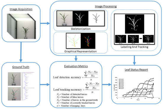
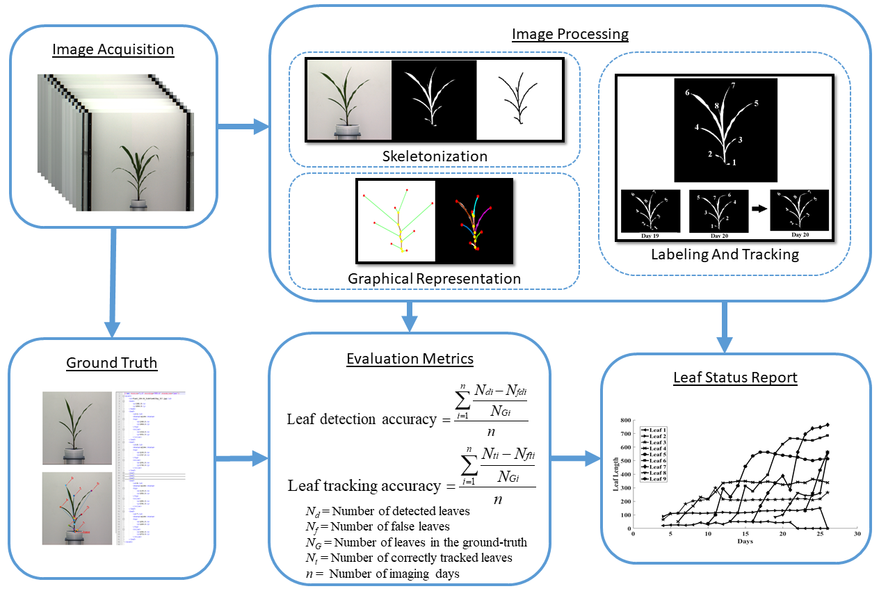
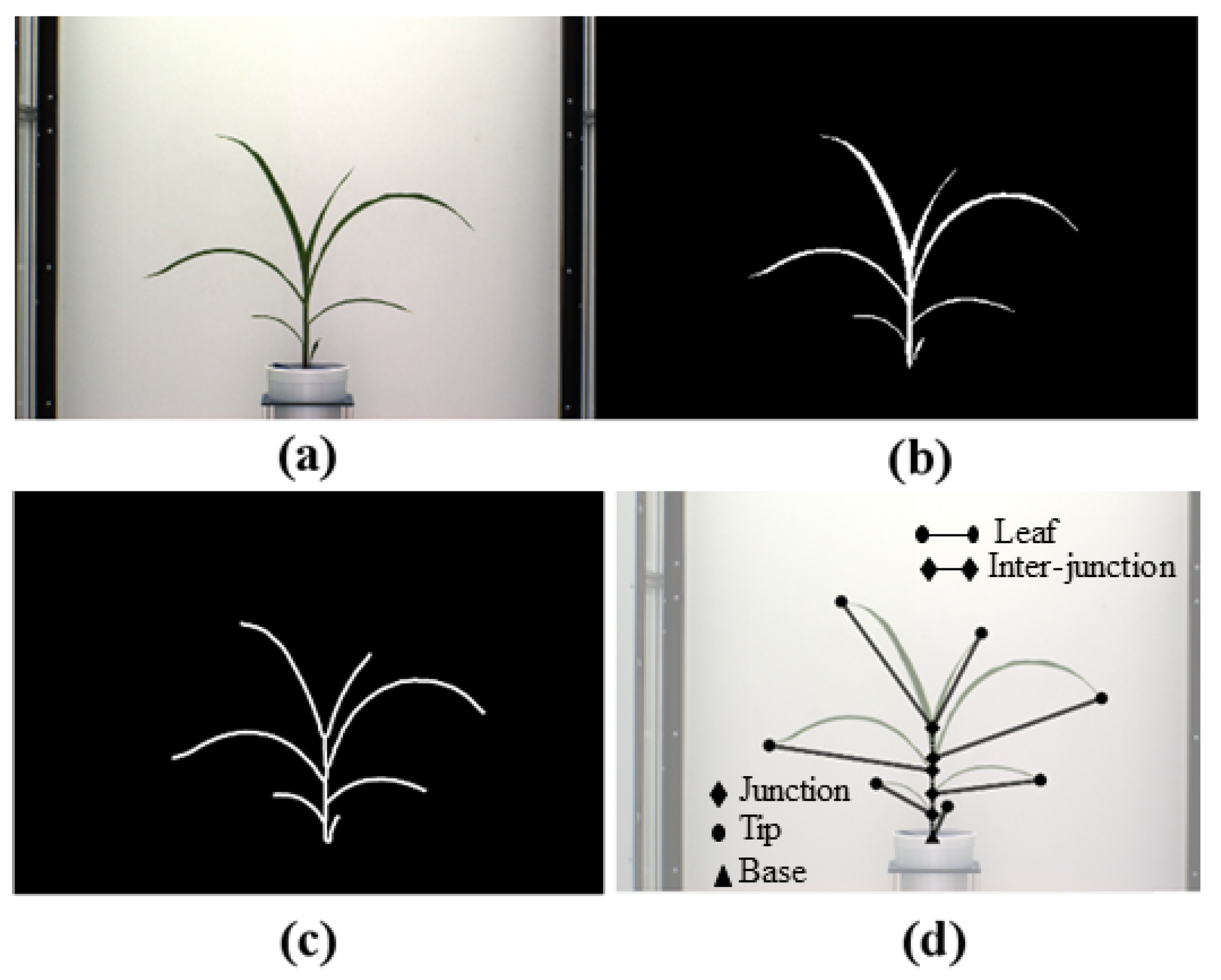
Figure 1 shows an overall image processing pipeline for the proposed method. Figure 1a shows the original image, and Figure 1b shows the corresponding binary image. The binary image is then skeletonized (see Figure 1c) to determine the graph representation of the plant, as shown in Figure 1d. Figure 1e shows each detected leaf is marked with a distinct color. Finally, Figure 1f shows each leaf numbered in order of emergence. The proposed method accepts a sequence of plant images captured at regular intervals over the vegetative stage life cycle of a plant as the input and generates a leaf status report along with a visual representation that encode the dynamic properties of all leaves that emerged during this period. The embedded phenotypic information is useful to plant scientists to provide greater understanding of the underlying physiological processes. This novel objective is achieved in four phases:
- View selection: Each plant is captured from multiple viewpoints to get a more accurate representation. We select the view at which the leaves are most distinct.
- Plant architecture determination: For each image in the sequence, we determine the architecture of the plant using a graph theoretic approach.
- Leaf tracking: The plant architectures are reconciled to determine the correspondences between the leaves over time to track them over the vegetative stage life cycle and demonstrate the temporal variation of the leaf-based phenotypes.
- Leaf status report: A leaf status report is produced as an output of the algorithm containing phenotypic information related to the entire life history of each leaf that best contributes to assessing plant vigor.
3.1. View Selection
Many plants alter leaf positioning (i.e., phyllotaxy) in response to light signals to optimize light interception [15]. To determine a plant’s architecture, the accurate location of the junctions (or collars, i.e., the points of contact of the leaves to the stem) and the tips (free endpoints of the leaves) is critical. Therefore, each plant is imaged from multiple viewpoints. The best view of the junctions is obtained in a view of the plant at which the line of sight of the camera is perpendicular to the axis of the leaves, as evident from Figure 2. In this view, the plant has the largest projection in the image. To determine this view, we first compute the area of the convex-hull of the plant for the available number of m views for the day the plant is imaged. The view at which the area of the convex-hull of the plant is the maximum, is selected for subsequent analysis. Given that a plant is imaged at m viewing angles each day, the optimal view () for day i is given by:
for i = 1, …, n, where n denotes the total number of imaging days, is the j-th view of the plant on day i, and the function returns the area of the convex-hull of the plant in the image.
3.2. Plant Architecture Determination
The steps for plant architecture determination are described below.
3.2.1. Segmentation
In a high-throughput phenotyping system, the plants are grown in a controlled environment like a greenhouse and imaged in a closed chamber. Thus, the imaging environment remains consistent in both camera and plant locations. Therefore, a frame-differencing approach using background subtraction gives a good approximation of the segmented plant [14]. This is followed by color-based thresholding to extract the foreground, i.e., the plant. A simple erosion removes noisy pixels, and a dilation step is used to fill in any small holes inside the plant image. At the end, the largest connected component in the image is deemed to be the plant.
3.2.2. Skeletonization
Skeletonization, i.e., the process of reducing a shape into one pixel wide connected lines, is widely used in object representation and recognition, character recognition, image retrieval, biomedical image processing, and computer graphics. Since many plants, including grasses such as corn and sugarcane, have elongated primary structures (stem, leaves, etc.), the skeleton provides the basis for the plant’s architecture.
Skeletonization algorithms are mainly based on morphological operations, discrete domain analysis using the Voronoi diagram, and fast marching distance transform. The morphological thinning-based methods iteratively peel off the boundary layer by layer, identifying the points whose removal does not affect the topology. Although straightforward, it requires extensive use of heuristics to ensure the skeletal connectivity, and hence does not perform well in the case of complex dynamic structures like plants. The geometric methods compute the Voronoi diagram to produce an accurate connected skeleton from the connected component. However, their performance largely depends on the robustness of the boundary discretization and is computationally expensive. We propose the use of fast marching distance transform to skeletonize the binary image [16] of the plants due to its robustness to noisy boundaries, low computational complexity, and accuracy in preserving skeleton connectivity structures.
The skeletonization process often results in the formation of unwanted spurious branches or spurs, which, in our application, can be erroneously identified as leaves [17]. The proposed method uses a thresholding-based skeleton pruning technique to remove spurs, i.e., if the length of the edge is less than the threshold value, it is considered as a spur, and hence discarded. The threshold can be determined through experimentation or using a supervised learning approach. Based on the experimental analysis of our dataset, we set the threshold value as 10 pixels, as this value removes spurs from all images of the dataset. Irrespective of the method chosen, in rare cases, this process will eliminate true leaves, when they are very small, right after emergence. However, leaves are dynamic structures; they will grow and be identified accurately in the image at the next time point.
Graph representations of skeletons have been investigated in the literature in many object recognition problems [18]. The method in [18] uses a skeletal graph to model a shape in order to use graph matching algorithms to determine similarity between objects. In this paper, we propose a graph representation for a plant. The plant structure lends itself naturally to such a representation since it consists of branches emerging from the main trunk and sub-branches emerging from branches and so on. Thus, the points where branches connect (and their ends) can be represented as nodes on a graph, and the branches (and leaves) and the internode segments in the stem can be represented as edges. The skeleton of the plant already is a good starting point to develop the graph representation. Furthermore, the use of graphs makes it efficient to decode the underlying structures (e.g., leaves and branches), and hence easier to track the dynamic properties of plants at a high level.
Before we formally introduce the algorithm for plant architecture determination, we define a few basic terms and show them graphically in Figure 1d.
- Base: The base of the plant is the point from which the stem of the plant emerges from the soil and is the lowest point of the skeleton.
- Collar/junction: The point at which a leaf is connected to the stem. The junctions, i.e., collars, are nodes of degree 3 or more in the graph.
- Tip: The free end of the leaf that is not connected to the stem.
- Leaf: The segments of the plant that connect the leaf tips and collars on the stem.
- Inter-junction: The segments of the plant connecting two collars are called inter-junctions.
A number of important properties of a plant can be directly identified from the graph representation. For example, the leaf tips and the base are nodes with a degree of 1, and the collars are nodes of degree 3. There are two types of edges in the graph: (a) leaves and (b) inter-junctions. Similarly, the stem of the plant can be formed by iteratively traversing the graph from the base along a connected path of collars.
Formally, we represent the plant by a graph , where V and E denote the set of vertices and the set of edges, respectively. The set of vertices is defined as , where B is the base of the plant, T is the set of the tips of the leaves, and J is the set of collars. The set of edges is defined as , where L and I represent the set of leaves and inter-junctions, respectively.
Algorithm 1 outlines the steps used for the determination of a plant’s architecture. We begin with a sequence of images of a plant P. Without loss of generality, we assume that the plant is imaged on a regular daily interval starting with Day 1. Thus, }, where is the image of the plant on day i and n is the number of days the plant was imaged. After view selection, each image is segmented to generate a sequence of segmented images .
Each segmented image is then skeletonized. The skeleton is transformed into a graph representation after the removal of spurious branches. The vertices and edges of the graph are directly determined from the skeleton. As described before, the vertices of the graph with a degree of 1 represent either the tip of a leaf or the base of the plant. Since the base of a plant holds a unique landmark in a plant, we first identify it. The base is determined by examining the degree one nodes (the base must have one of the lowest y-coordinates) and the edge that connects to the plant (it must be a straight line segment that is close to vertical). These special conditions are needed since a leaf may droop in such a way that its tip may fall below the base.
Once the base is determined, the next step is to determine the stem of the plant since all leaves emerge from it. We again leverage the structure of the stem, i.e., it is straight and consists of inter-node segments. Thus, starting from the base and following the edges, neither of whose nodes has degree one (collar), generates the stem of the plant. This is summarized in Algorithm 2. After the stem is identified, we determine the orientation of each leaf. In the maize plant, the leaves emerge in alternate-opposite orientation. Without loss of generality, we assign the leaves emerging to the left as 0 and those emerging to the right as 1.
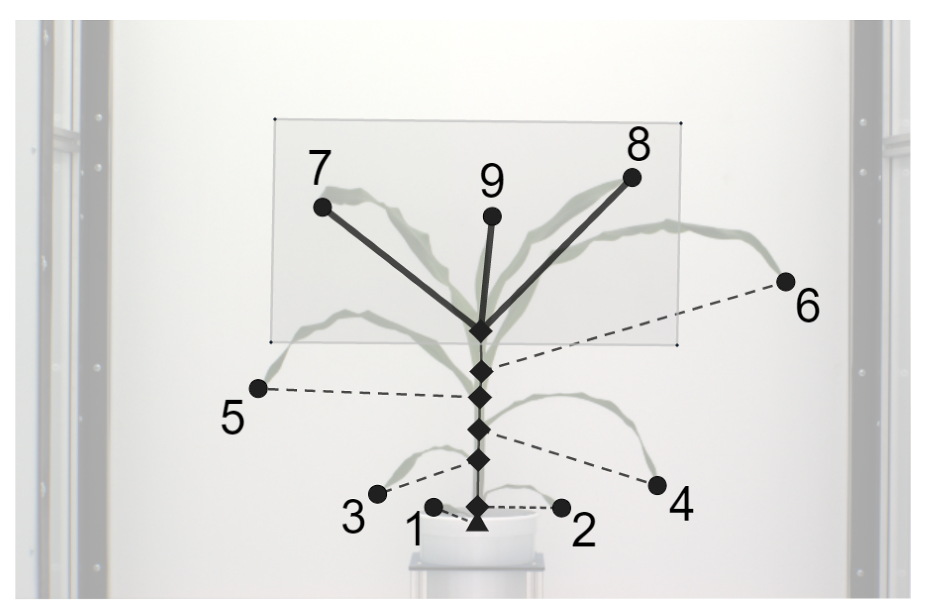
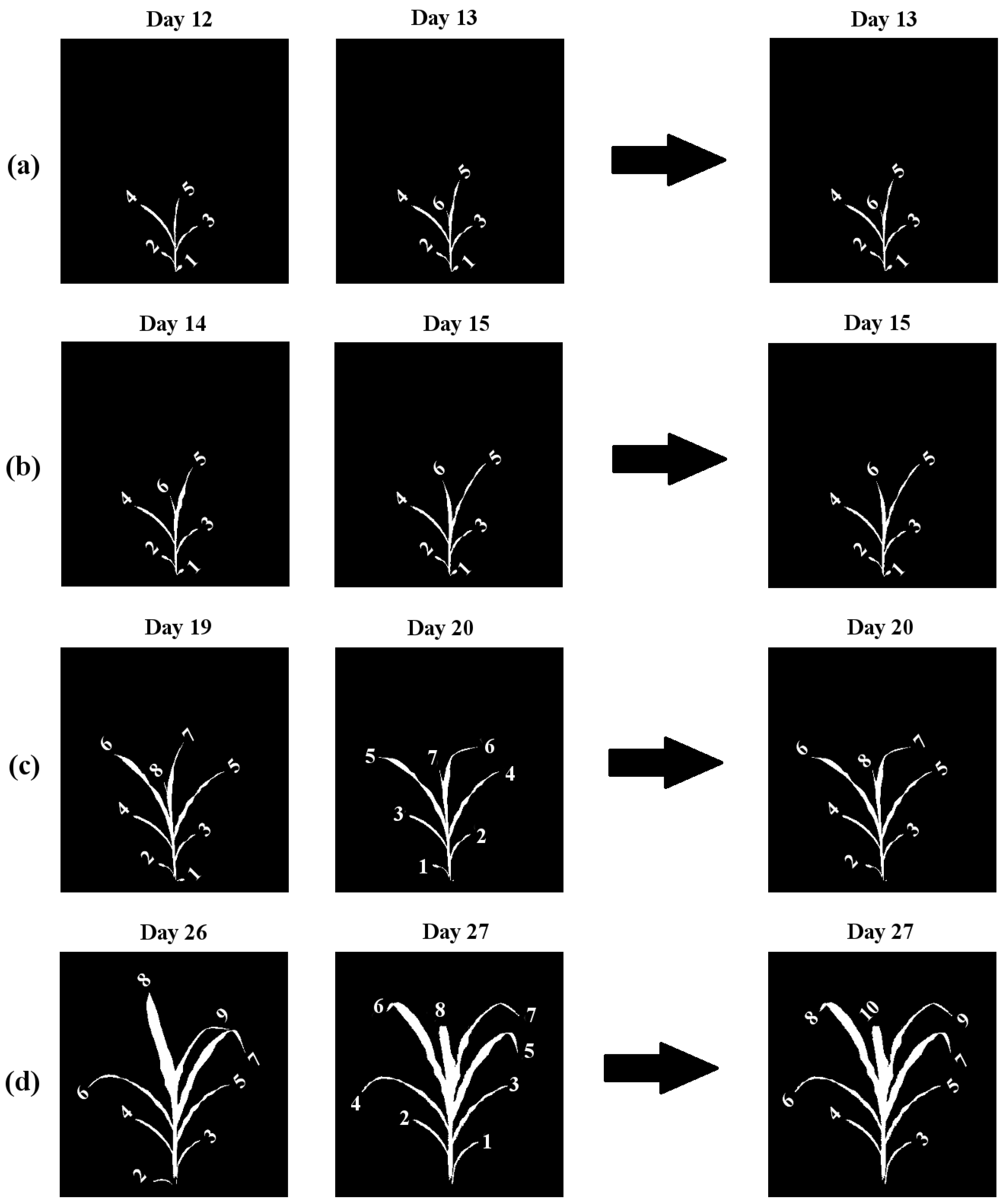
The final step in the plant architecture determination is the identification of the leaves and labeling them in emergence order. We use two properties of the plant growth in this process: (a) the order of the emergence of leaves in the plant is bottom to top; (b) a new leaf emerges on the opposite side of the last leaf in the plant; and (c) older leaves are typically longer than newer leaves. Thus, the oldest leaf is closest to the base of the plant and the newest the farthest. Hence, our algorithm follows the stem from the base and, at each collar (c), determines the leaves present by identifying the edges with one vertex as the collar and a leaf tip as the other vertex (degree 1 vertex). A counter (label) is used to keep track of the label for the next leaf in the emergence order. If there is only leaf present at the collar, then it is labeled with the value of the counter, and the counter is incremented. It is possible, however, that in some cases, typically the last collar, multiple leaves may be connected to a single collar (see Figure 3). In such a case, we use the constraint that the next leaf to be the longest leaf in the set has the orientation opposite the previous leaf. This process is repeated until all the leaves in the set are labeled. Figure 4 shows the process of the graph representation of a plant from the original image.
| Algorithm 1 Plant architecture determination: produces a graphical representation of all the images of a plant sequence to detect the leaves and stem. |
| Input: The image sequence of a plant, i.e., } Output: G = {, , …, }, where is the graphical representation of the i-th image ∀i = 1,…, n. for do { // segment the image for day i // compute the skeleton of the segmented image . = // remove spurious edges with a threshold of pixels. // represent the plant skeleton as a graph // vertices and edges of the graph // degree 1 vertices // find the base ; // tips of the leaves // collars or junctions ; // Assign orientation to each leaf count = 1; // starting label for leaves for do { // follow junctions starting from base []=; // extract the vertices from edge if () continue; if () { // there is only one leaf at the junction .label = count; count ++; } else { // there are multiple leaves at the junction orient = count //previous leaf orientation orient = ¬ orient; // next leaf orientation leaves = // initialize with the leaves at the node while (l) do { // orientation of the next leaf // remove the leaf count ++; end while end for end for |
| Algorithm 2: determine the stem in a graph. |
| Input: A graph G and its base B. Output: A list of edges in G that constitute the stem (S). v = B; done = FALSE; S = []; while (¬ done) { = ; // find the non-visited adjacent vertex of degree ≠ 1 if ( = NULL) // there is no adjacent vertex with degree ≠1 done = TRUE; else{ S.append() // add the inter-stem segment to the stem ; } } |
3.3. Leaf Tracking
Each leaf in a plant has a unique time of emergence, pattern of growth, and senescence. We, therefore, assign each leaf a label that determines its emergence order. Thus, the leaf that emerged first will be labeled 1 throughout the life of the plant, even if the leaf may die. Thus, the leaf tracking problem is equivalent to the determination of the correct label for each leaf in the plant in a sequence of plant images. The correspondence between the leaves in any two images (or any sequence of images) can be directly determined from the labels.
Our leaf tracking algorithm is based on the following set of properties that hold for a large class of plants including grasses like maize.
- A new leaf emerges above the last leaf in opposite alternate orientation, i.e., if the previous leaf emerged from the left side, the next leaf will emerge from the right side and will originate from a collar situated above the collar of the immediate previous leaf.
- In the event of a loss of a leaf, the height of its collar decreases, and the length of the corresponding inter-junction increases compared to the previous image.
In addition, we make the following assumptions, which hold in most high-throughput phenotyping systems, where each plant is imaged on a daily scale.
- No more than one leaf may die in two consecutive images in a sequence.
- No more than one new leaf may emerge in two consecutive images in a sequence.
Based on these properties, only four scenarios are possible when examining an image in a sequence with respect to the previous image (illustrated in Figure 5).
- 1
- Leaf emergence: A new leaf emerged, but no leaf was lost (Figure 5a).
- 2
- No change: No new leaf emerged, and no leaf was lost (Figure 5b). In this case, we transfer the labels from the previous graph to the next graph.
- 3
- Leaf loss: A leaf was lost, but no new leaf emerged (Figure 5c).
- 4
- Loss and emergence: A new leaf emerged, and a leaf was lost (Figure 5d).
Algorithm 3 summarizes the leaf tracking process for the plant image sequence using graphs generated by Algorithm 1. The leaf tracking algorithm begins with a sequence of labeled graphs {}, where is the graph for day i for a plant and n is the number of days the plant is imaged. The leaves for each plant in the graph are labeled starting with 1, as each plant was labeled independently. The problem of tracking reduces to finding the correspondence between the leaves of two consecutive plants, i.e., graphs and . We assume that has been properly labeled, and we must label . As stated before, since the plants are imaged frequently, the change in , if any, can come in the form of either a new leaf or a dead leaf or both.
New leaf: Since new leaves always emerge from the last collar, the newest leaf in a plant will have the highest label in its corresponding graph. Given graphs and , if the leaves with the highest labels in the two do not match in the image, then a new leaf has emerged in . Matching can be done by simply matching their orientations. Thus, has a new leaf with respect to , iff:
where lastLeaf returns the leaf (edge in a graph) whose label is the highest. In this case, each label of the leaves in is incremented by the label of the first leaf in .
Dead leaf: Similarly, the oldest visible leaf in a plant will have the lowest label, in its corresponding graph. Thus, if the leaves with the smallest labels do not align in graphs and , then a leaf in has been lost in . In such a case, the first leaf will not align with the first leaf (Leaf 1) . Again, the alignment can be done by simply matching their orientations. Thus, has lost a leaf with respect to , iff:
where firstLeaf returns the leaf (edge in a graph) whose label is the smallest. In this case, the labels for the rest of the leaves in are transferred from .
Table 1 summarizes the four possible scenarios when tracking the leaves from to .
The leaf tracking process is summarized in Algorithm 3. We assume that is correctly labeled. We then update the labels for from starting with . At each step, we first examine if a leaf has been lost or if a new leaf has emerged. If no leaf has been lost, we simply update the labels of the leaves in , by incrementing them by the label of the first leaf of (). If, however, a leaf is lost, the increment term () is the label of the second leaf in .
| Algorithm 3 Leaf tracking algorithm. |
| Input: G = {, , …, , …, }, where is the graphical representation of the i-th image ∀i = 1,…, n, obtained from Algorithm 1. Output: = {, , …, , …, }, where is the graphical representation of the i-th image ∀i = 1,…, n, with the leaves correctly tracked and labeled. for do { lostLeaf = checkLostLeaf(, ); // See Equation (3) if (¬ lostLeaf) = firstLabel(); else = firstLabel() + 1; = updateGraph(, ); end for |
3.4. Leaf Status Report
Once all the leaves are tracked from their emergence over the life cycle of the plant, a leaf status report can be generated to provide significant phenotypic information based on the property of each leaf. For this paper, we report the length of the leaves, which may be replaced or augmented with other phenotypes (e.g., curvature) seamlessly. The steps to compute the length of a leaf are as follows.
Leaf Length
Leaf length can be computed by counting the number of pixels for an edge in the graph in the corresponding skeleton segment. A more accurate approach may use a curve fitting approach as follows. Let the n-th order polynomial curve p for each leaf be given by:
where , , …, are the coefficients of the best fit polynomial for the leaf skeleton optimizing the least squares error. The leaf length is measured by:
where and denote the x-coordinates of the collar and tip for the leaf, respectively.
The leaf status report displays the phenotypic information of each leaf as a function of time throughout its life. It explicitly provides the following phenotypic information, which is significant in the context of plant sciences: (a) the total number of leaves emerged during the life cycle, (b) the day on which a particular leaf emerged, (c) the number of leaves present at any point of time, (d) the length of each leaf at any point of time, (e) the day on which a particular leaf died, and (f) the rate of growth of each leaf.
3.5. Evaluation Metrics
The success of the leaf tracking algorithm depends on how accurately the leaves are detected. Thus, the performance of the proposed method is evaluated using two criteria, i.e., leaf-detection accuracy (LDA) and leaf-tracking accuracy (LTA). These are defined below.
- Leaf-detection accuracy (LDA): The leaf-detection accuracy and leaf-tracking accuracy are respectively given by:where , , and are the number of detected leaves, the number of false leaves, and the actual number of leaves (as noted in the ground truth) for the i-th day for a given plant. This is computed for each plant separately.
- Leaf-tracking accuracy (LTA): This measures the accuracy of our leaf tracking algorithm and is given by:where , , and are the number of correctly tracked leaves, the number of wrongly tracked leaves, and the actual number of leaves (as noted in the ground truth) for the i-th day for a given plant, respectively. This is also computed for each plant separately.
4. UNL-CPPD
The performance of the algorithm is evaluated based on experimental analyses on the UNL-CPPD. The UNL-CPPD is introduced to stimulate research in the development and comparison of algorithms for leaf detection and tracking, leaf segmentation, and leaf alignment of cereal crops, e.g., maize and sorghum [8].
4.1. Imaging Setup
The UNL-CPPD was created in a greenhouse equipped with a Lemnatec Scanalyzer 3D high-throughput plant phenotyping facility at the center for plant science innovation at the University of Nebraska-Lincoln (UNL), USA. The facility is managed by the Argus environmental control system that controls heating, air conditioning, light timing, roof vent opening, etc., and records greenhouse temperature, humidity, light intensity, and atmospheric pressure. Each pot is fitted in a metallic/composite carrier, which was placed on the automated conveyor belt that moves the plant (of height up to 2.5 m) from the greenhouse to the imaging cabinets in succession for capturing images in different modalities, i.e., visible light (side view and top view), fluorescent (side view and top view), infrared (side view and top view), hyperspectral (side view), and near-infrared (top view). Each imaging chamber has a rotating lifter, which rotates the plant in front of the camera for up to 360 side view images. The conveyor belt has the capacity to accommodate a maximum number of 672 plants. It has three watering stations that water the plants on a daily basis to the target weight or a specific volume. The target weight can be increased as plants grow to compensate for increased mass.
4.2. Dataset Organization
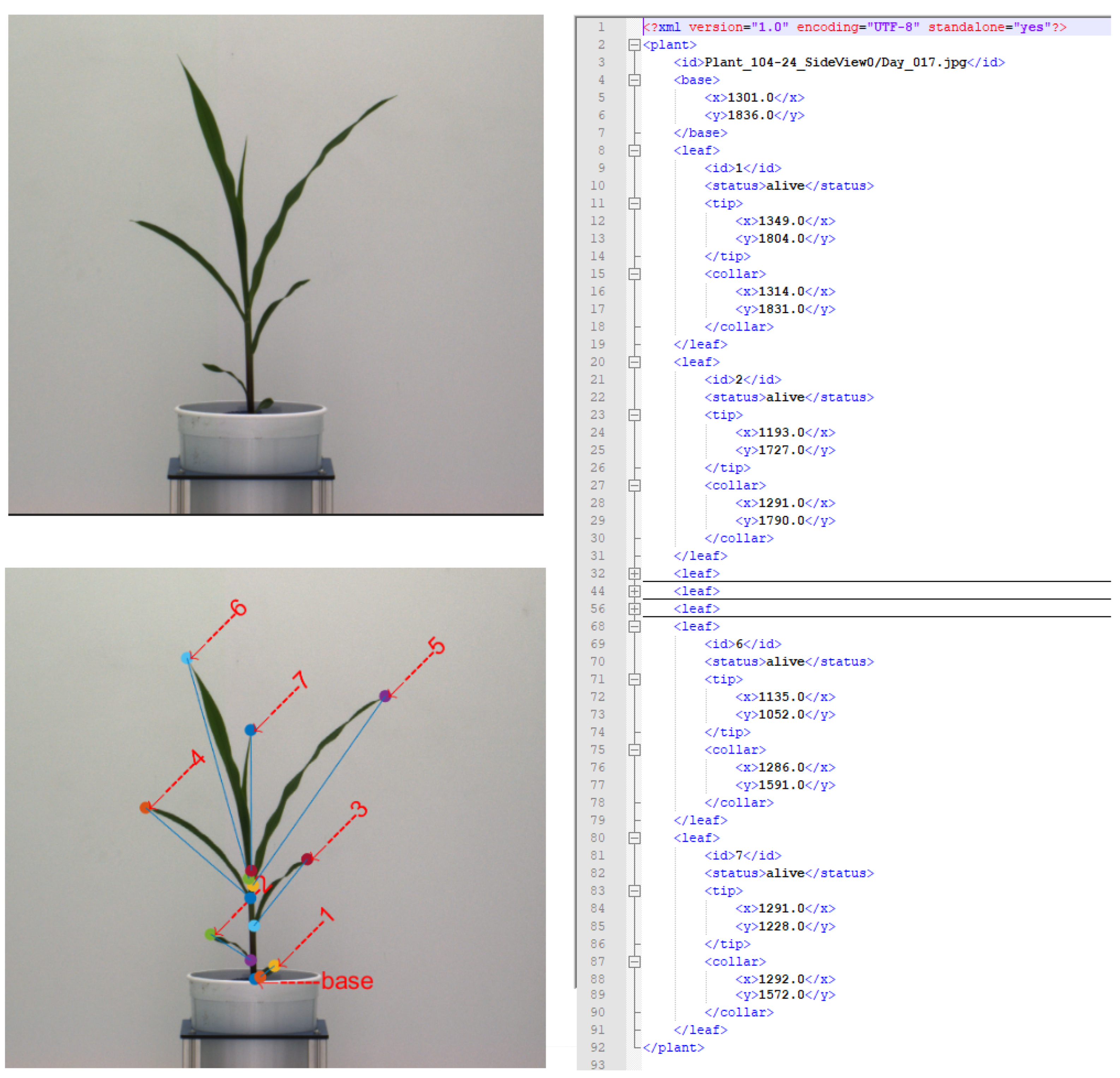
The UNL-CPPD has two versions: UNL-CPPD-I (small) and UNL-CPPD-II (large). UNL-CPPD-I consists of images of 13 maize plants for 2 side views, i.e., 0 and 90, captured by the visible light camera once daily for 27 days, starting from two days after germination, which merely excludes self-occlusions due to crossovers. UNL-CPPD-II is comprised of images of the same 13 plants for the same two views, but for a longer duration, i.e., 32 days, which includes images of plants with leaf crossovers and self-occlusions [8]. Each image of the UNL-CPPD dataset is accompanied by the ground truth in the form of: (a) an XML document that embeds the information about the plant id, the coordinates of the base of the plant, the information about the leaves including the leaf number (in order of emergence), the coordinates of the base, collars, and tips, and if the leaf is alive, missing, or dead; and (b) an annotated image with each leaf numbered in order of emergence [8]. The leaf emergence order was visually tracked during a plant’s growth process and recorded. This knowledge was used to create the annotated image sequence of the plant to serve the purpose of the ground truth for leaf tracking. We customized the web-based image annotation tool called LabelMe [19] to meet our requirements for ground truth generation. The labels, i.e., the co-ordinates of the base, collar, and tips, were created by manually clicking on those points. While clicking, the values of their coordinates are automatically stored in the XML file format, which makes the annotations portable and easy to extend.
Figure 6 shows an original image from UNL-CPPD-I and its ground truth, i.e., the annotated image and the XML document. The root element of the XML document is Plant, which has three child elements, i.e., id, base, and leaf [8]. The interpretations of these elements are provided below.
- Id: It serves two purposes based on its placement. If it is inside the Plant element, it serves the purpose of the image identifier, i.e., the day and the view of the image for which the information is represented in the XML document. When placed inside the Leaf element, it refers to the leaf number in order of emergence.
- Base: It has two attributes, i.e., x and y, which represent the pixel coordinates for the location of the base in the image.
- Leaf: It has four children, i.e., id, status, tip, and collar. id refers to the leaf emergence order, and status represents the status of the leaf (alive, dead, or missing). status “alive” means the leaf is visible in the image connected to a collar. status “dead” means that the leaf appears to be dead in the image mainly due to the separation from the stem. status “missing” means the leaf is no longer visible in the image either due to shedding or occlusion at a particular view. The tip element has children x and y, which represent the coordinates of the pixel location of the leaf tip; similarly, the collar element represents the coordinates of the pixel location of the junction.
5. Results
We evaluated the performance of the proposed method using UNL-CPPD-I and provide improvement directions to handling the leaf tracking challenges due to the presence of intersecting leaves using UNL-CPPD-II. The results of the evaluation in terms of LDA and LTA are discussed. We also demonstrate the benefit of the leaf status report in this section.
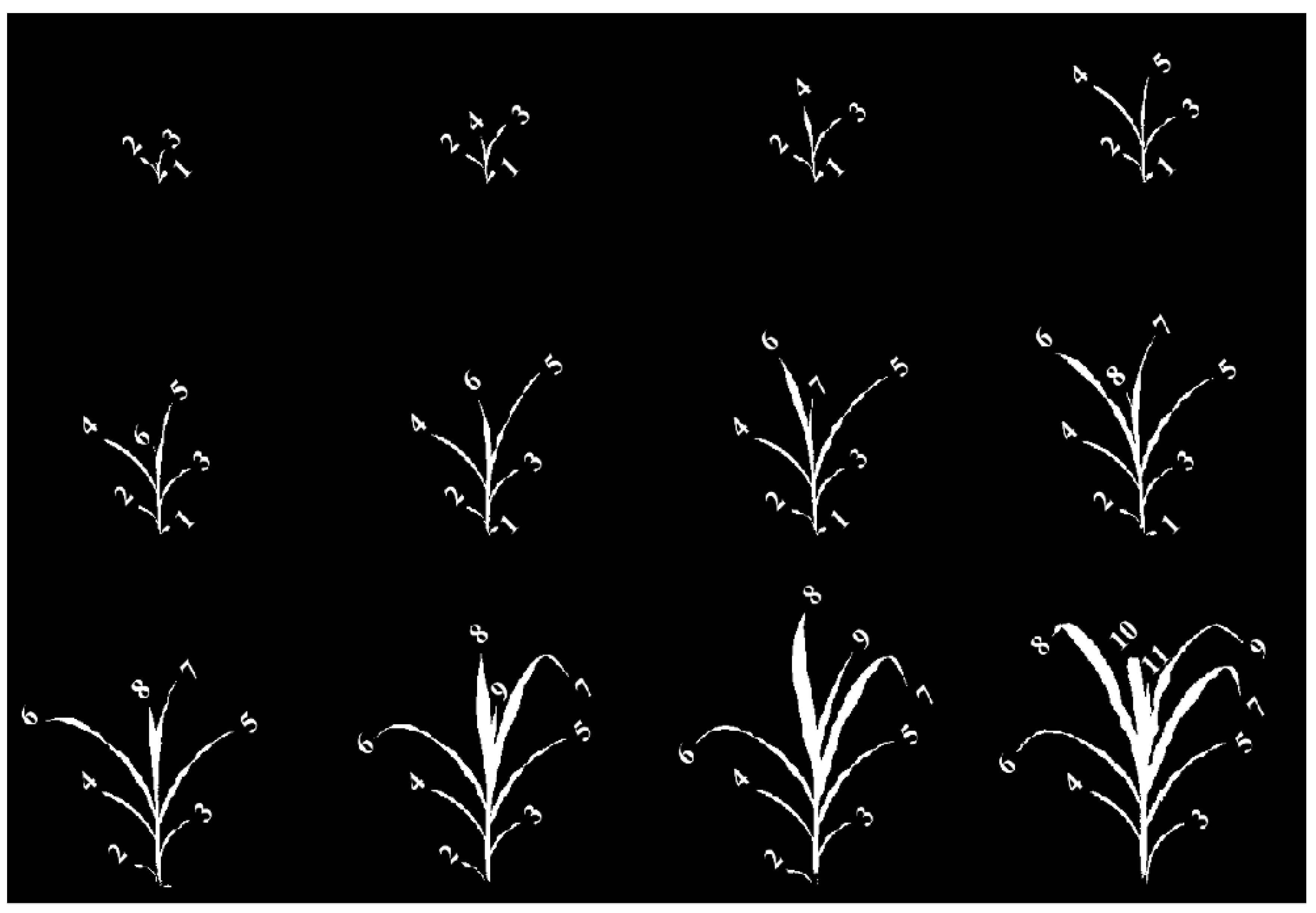
Table 2 shows the results of the experimental analyses of the proposed method on UNL-CPPD-I. In the case of seven out of 13 plant sequences, all leaves were tracked correctly, showing 100% LTA. However, the poor performance of and in terms of LTA was attributed to the fact that a failure in the detection of a leaf in the early stage rendered the tracking of leaves wrong throughout the life cycle. The proposed method achieves promising LTA for the remaining four sequences. The table shows that the average LDA is 92%, whereas the average LTA is 88%. Figure 7 shows the results of tracking using a plant sequence () from UNL-CPPD-I.
5.1. Leaf Status Report
Figure 8 shows the leaf status report generated for a plant sequence (i.e., ) in the dataset. Each leaf in the plant is represented by a graph. The axes of the graphs are time (in days) and phenotype (leaf length). The report shows the dates of emergence of the leaves, e.g., Leaf-1 emerged on Day 4, whereas Leaf-5 emerged on Day 10. Furthermore, we can get information on the length of each leaf on any given day, e.g., the length of Leaf-4 on Day 10 is 180 pixels. The report shows that senescence (death) for Leaf-1 occurred on 22 and Leaf-2 on Day 26. It is evident from the report that the growth of the leaves that emerged later in the plant’s life was significantly higher compared to the leaves that emerged during the early phase of the plant. One possible explanation for this pattern is the reduction in the amount of sunlight received by the lower leaves as they grow under the upper leaves. Note that for some days, the length of a leaf decreases from the previous day, e.g., Leaf-4 on Day 10. Some factors that influence this include plant rotation, occlusion, and the fact that that the measurements are made from the 2D projection of the 3D leaves.
5.2. Limitation Handling
The growth pattern in the early plant stages provides critical phenotypic information related to yield, and hence is of most interest to plant scientists and agronomists. The early growth stages are characterized by the absence of self-occlusions and leaf crossovers, and the proposed method achieves high proficiency in tracking the leaves in that scenario. However, the architectural complexity of plants increases with time due to the development of new organs, resulting in more frequent occlusions and crossovers. With a limited number of views, the determination of the plant architecture based on skeleton-graph transformation becomes increasingly challenging in the late vegetative stages.
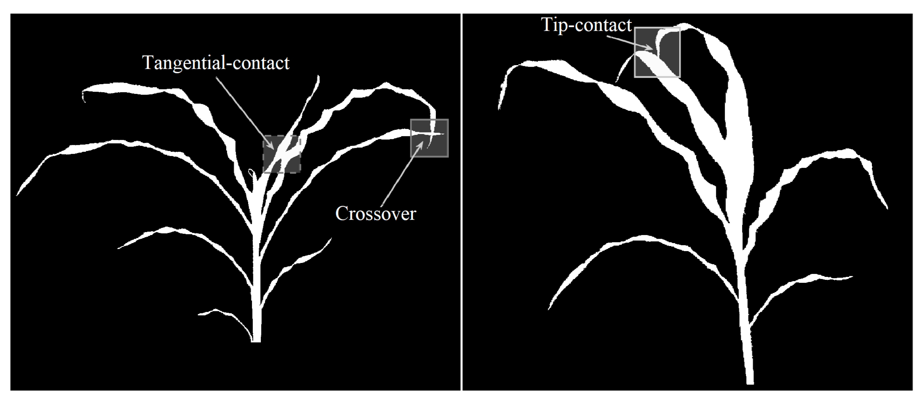
When two leaves in a plant intersect, their representations in the skeleton-graph share one or more nodes. Furthermore, the skeleton-graph is no longer a tree since it contains one or more loops due to the intersections. Based on the nature of the contact between the leaves, the intersections are classified into three types: (a) tip-contact, (b) tangential-contact, and (c) crossover. Figure 9 shows examples of these cases where the proposed algorithm fails to track the leaves accurately. The proposed method can be extended to address the above three failure cases by leveraging the growth characteristics of the leaves, i.e., the leaves represented as the edges in the skeleton-graph must demonstrate angular consistency.
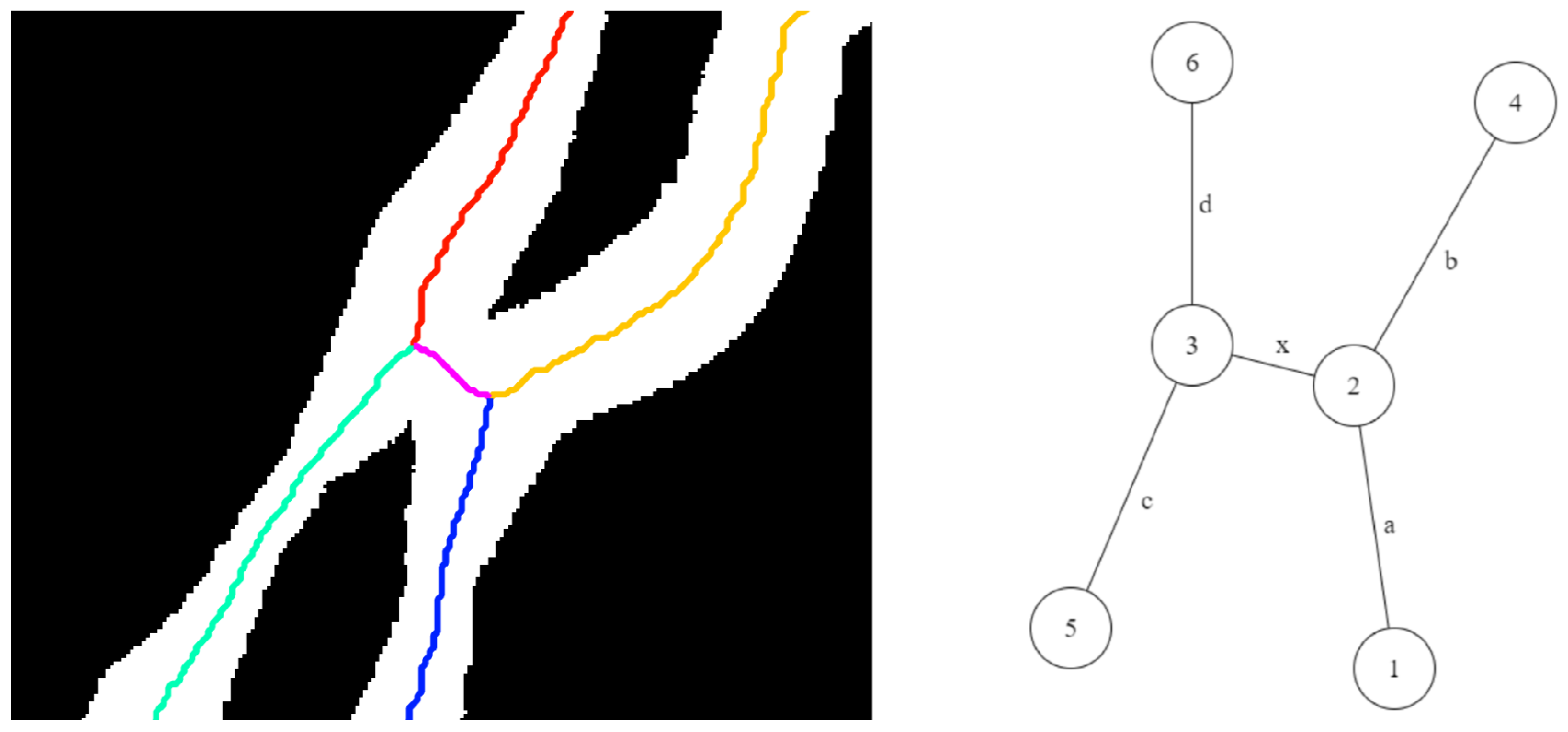
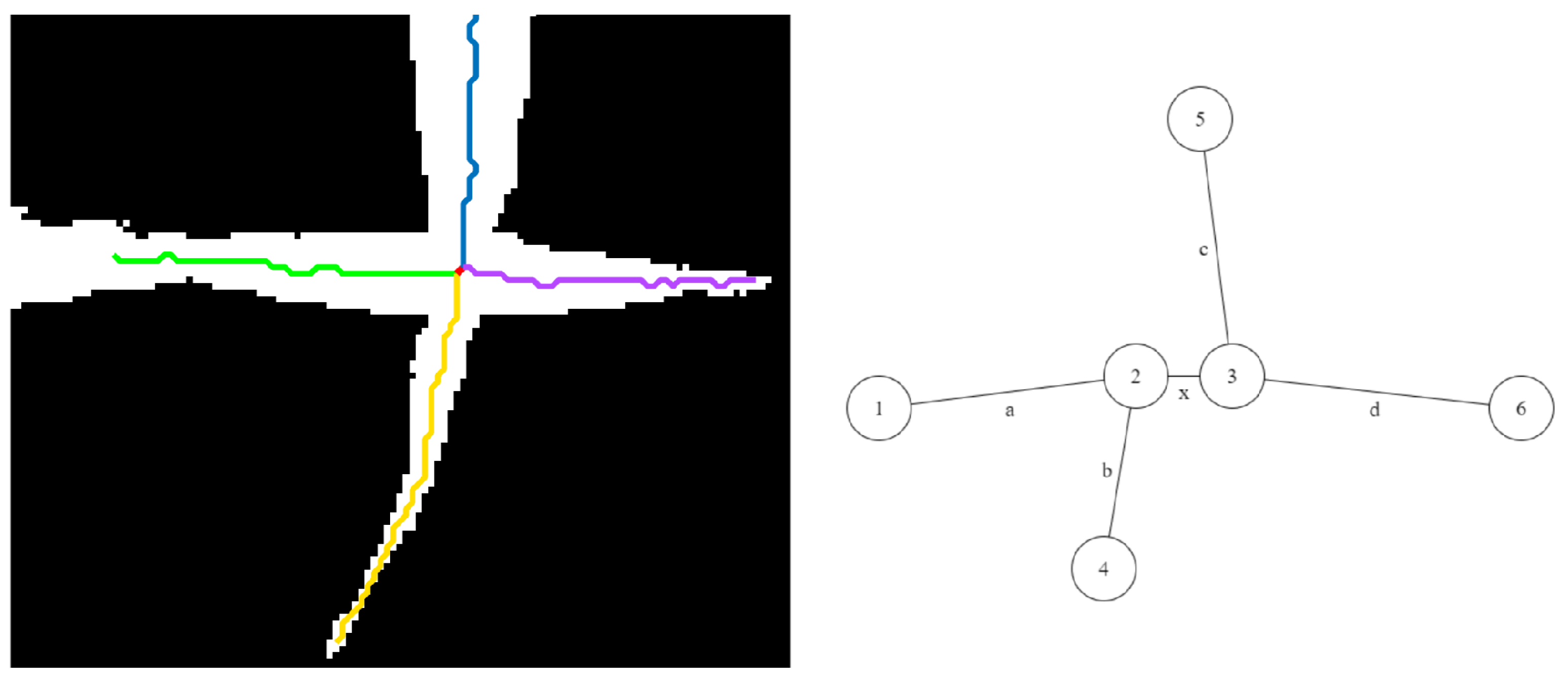
The proposed algorithm tracks each leaf starting from its junction, using a bottom-up approach, by following the edge until it reaches a tip (degree one node). When there is no leaf intersection, only degree two nodes are encountered along the way. In the presence of leaf intersections, the algorithm encounters higher degree nodes and must select the edge that represents the continuation of the current leaf. A look-ahead approach is used to determine the next node in the path, i.e., we select the node that provides the highest continuity, measured by angular consistency, with the leaf segment traced so far. Figure 10, Figure 11 and Figure 12 illustrate this process for three common scenarios of leaf intersections, i.e., tangential-contact, tip-contact, and crossover, respectively. In every case, the algorithm starts with Node 1, follows edge a, and reaches Node 2, a degree three node. The algorithm must now choose between two nodes: Node 3 and Node 4 as the continuation of the current leaf. Depending on the degrees of these two nodes, the following two scenarios can arise:
- (1)
- Case A: The degrees of both the nodes are less than three. This case corresponds to the scenarios shown in Figure 10. In this case, the node with the most angular consistency with edge a is chosen. In Figure 11, Node 3 is selected, and edge b is marked with the current leaf number. When Node 2 is reached via edge c, the algorithm stops tracking since there are no unseen edges to follow, and it labels it as the tip for that leaf.
- (2)
- Case B: One node has degree three, and the other has degree two or less: This case may correspond to the scenarios in either Figure 11 or Figure 12. In this case, a two node look-ahead (from the new degree three node) is performed to identify all combinations of edges that form a path from Node 1 to the resulting nodes from the second look-ahead. The path with the highest angular consistency is chosen to continue the current leaf.Depending on the type of intersection, edge x is either shared (in the case of a crossover) or ignored (in the case of a tangential contact) for detecting leaves accurately. In Figure 10, the possible leaf segments are {}, and the path is selected for the highest angular consistency. When the algorithm reaches Node 5 from Node 3 following edge b, a similar analysis will continue the leaf to Node 6 using edge d, and edge x will remain unused and eventually ignored by the algorithm. For the scenario in Figure 12, however, with the same set of possible leaf segments, i.e., {}, the path is chosen for the highest angular consistency. When the algorithm reaches Node 2 from Node 4, the same analysis will select as the best path for leaf continuation, in essence sharing edge x. Thus, the leaves are detected accurately in the presence of different types of intersections.
6. Discussion
Leaves are one of the primary organs of plants that transform solar energy into chemical energy in the form of carbohydrates through photosynthesis, releasing oxygen as a byproduct. The total number, emergence timing, and size of leaves are therefore related to plant photosynthetic light efficiency and net primary productivity. Leaf stage monitoring of cereal crops plays a crucial role in the understanding of plant’s vigor and yield prediction modeling. The paper introduces a new concept of visual growth tracking to solve a previously unexplored topic of automated leaf stage monitoring of maize plants.
The proposed method is applicable for plants with distinct stems that are above ground, not highly branched, and characterized by distinct nodes and internodes. The skeletonization process plays a crucial role in the accurate determination of the plant architecture. The proposed method uses a threshold-based skeleton pruning technique to remove spurs based on experimental analysis tailored to a specific dataset. This spur removal process often eliminates true leaves along with the spurs when the leaves are very tiny after emergence. This reduces the LDA. However, for these cases, the older leaves that are detected can all be tracked successfully, resulting in a higher LTA. This explains the cases of the lower LDA for plants with 100% LTA in Table 2. Note that these newly emerged tiny leaves will grow in the later days to surpass the spur threshold and can be detected successfully. False leaf detection or failure in the detection of one or more older leaves due to crossovers and occlusions for the early days might result in inaccurate leaf tracking throughout the life cycle, and thus significantly reduce the LTA.
Presently, the method provides curve tracing solutions of three identified types of leaf intersections, i.e., tip-contact, tangential-contact, and crossover. This study is based on 13 maize plants only; hence, future work will consider the formation of a larger dataset for a detailed investigation to identify if there is any other type of leaf intersection that impacts the efficacy of the proposed method. Our future dataset will also include image sequences of other species sharing a similar architecture as maize, i.e., sorghum, for experimental evaluation. A plant’s overall growth is significantly impacted by environmental stress factors. The proposed method has the potential to investigate the effect of drought or thermal stress on leaf growth stages regulated by genotypes.
A fundamental challenge in computer vision is that images do not carry all the information about the scene that they represent. As the plants proceed through the late vegetative stages, their architectural complexity increases with a higher level of branching and self-occlusions. Therefore, accurate leaf detection and tracking from the 2D images of the plants, which are 3D in nature, become increasingly challenging. Hence, we will consider the reconstruction of a 3D model of a plant from multi-view image sequences in the future work to achieve robustness.
The proposed method was implemented using MATLAB R2016a on an Intel(R)Core(TM) i7 processor with 16 GB RAM working at 2.60-GHz using the 64 bit Windows 7 operating system. The average execution time of a single plant sequence consisting of 27 × 2 = 54 images was 15.38 min. The time included view selection, determination of individual plant architecture, leaf tracking, and leaf status report generation.
7. Conclusions
The paper introduces a novel method for automated tracking of individual leaves that change in size, shape, and structure over time, using multi-view image sequences of a plant for application in phenotyping. This is a pioneering study that replaces the manual and destructive process of growth stage determination of an economically important crop like maize. The method has four phases: (a) optimal view selection; (b) plant architecture determination based on a graph theoretic approach; (c) leaf tracking to assign labels to each leaf based on the order of emergence; and (d) the generation of the leaf status report. The method starts with an image sequence of a plant captured by a visible light camera as the input and produces a leaf status report containing phenotypic information useful to assess the plant vigor, i.e., the timing of the emergence and senescence of each leaf, the length of each leaf on a particular day, and the relative growth rates of individual leaves. The paper introduces a curve tracing technique based on an angular consistency check in an attempt to augment the proposed algorithm to address the challenge of intersecting leaves for robust leaf tracking. The method requires the availability of the image view of the plant at which the nodes (tips and junctions) are distinctively visible. The future work will consider the reconstruction of the 3D model of the plant from multi-view image sequences to address the challenges of intersecting leaves more efficiently.
Author Contributions
S.B. and S.D.C. developed and implemented the algorithm and led the experimental analysis and the manuscript writing. A.S. supervised the research and provided constructive feedback throughout the algorithm development process. A.S. and T.A. contributed to the manuscript writing. All authors contributed to the article and approved the submitted version. All authors have read and agreed to the published version of the manuscript.
Funding
This research is supported by the Nebraska Agricultural Experiment Station with funding from the Hatch Act capacity funding program (Accession Number 1011130) from the USDA National Institute of Food and Agriculture.
Institutional Review Board Statement
Not applicable.
Informed Consent Statement
Not applicable.
Data Availability Statement
The UNL-CPPD is freely available at https://plantvision.unl.edu/dataset (accessed on 1 March 2021).
Acknowledgments
The authors would like to thank the High-Throughput Plant Phenotyping Core Facility (Scanalyzer 3D, LemnaTec Gmbh, Aachen, Germany), located at the Nebraska Innovation Campus of the University of Nebraska-Lincoln, USA, for generating the images used in this study.
Conflicts of Interest
The authors declare no conflict of interest.
Sample Availability
A short video of the result is available at https://plantvision.unl.edu/projects-0 (accessed on 1 March 2021).
References
- Xing, J.; Ai, H.; Liu, L.; Lao, S. Multiple Player Tracking in Sports Video: A Dual-Mode Two-Way Bayesian Inference Approach With Progressive Observation Modeling. IEEE Trans. Image Process. 2011, 20, 1652–1667. [Google Scholar] [CrossRef] [PubMed]
- Jiang, Z.; Huynh, D.Q. Multiple Pedestrian Tracking From Monocular Videos in an Interacting Multiple Model Framework. IEEE Trans. Image Process. 2018, 27, 1361–1375. [Google Scholar] [CrossRef] [PubMed]
- Velazquez-Pupo, R.; Sierra-Romero, A.; Torres-Roman, D.; Shkvarko, Y.V.; Santiago-Paz, J.; Gómez-Gutiérrez, D.; Robles-Valdez, D.; Hermosillo-Reynoso, F.; Romero-Delgado, M. Vehicle Detection with Occlusion Handling, Tracking, and OC-SVM Classification: A High Performance Vision-Based System. Sensors 2018, 18, 374. [Google Scholar] [CrossRef] [PubMed] [Green Version]
- Min, W.; Fan, M.; Guo, X.; Han, Q. A New Approach to Track Multiple Vehicles With the Combination of Robust Detection and Two Classifiers. IEEE Trans. Intell. Transp. Syst. 2018, 19, 174–186. [Google Scholar] [CrossRef]
- Yin, X.; Liu, X.; Chen, J.; Kramer, D.M. Joint Multi-Leaf Segmentation, Alignment, and Tracking from Fluorescence Plant Videos. IEEE Trans. Pattern Anal. Mach. Intell. 2017, 40, 1411–1423. [Google Scholar] [CrossRef] [Green Version]
- Cakir, R. Effect of water stress at different development stages on vegetative and reproductive growth of corn. Field Crop. Res. 2004, 89, 1–6. [Google Scholar] [CrossRef]
- Hardacre, A.K.; Turnbull, H.L. The Growth and Development of Maize (Zea mays L.) at Five Temperatures. Ann. Bot. 1986, 89, 779–787. [Google Scholar] [CrossRef]
- Choudhury, S.D.; Bashyam, S.; Qui, Y.; Samal, A.; Awada, T. Holistic and Component Plant Phenotyping using Visible Light Image Sequence. Plant Methods 2018, 19, 174–186. [Google Scholar] [CrossRef]
- Vylder, J.; Ochoa, D.; Philips, W.; Chaerle, L.; Straeten, D. Leaf Segmentation and Tracking using Probabilistic Parametric Active Contours. Vis. Comput. Graph. Collab. Tech. 2011, 6930, 75–85. [Google Scholar]
- Scharr, H.; Minervini, M.; French, A.P.; Klukas, C.; Kramer, D.M.; Liu, X.; Luengo, I.; Pape, J.; Polder, G.; Vukadinovic, D.; et al. Leaf segmentation in plant phenotyping: A collation study. Mach. Vis. Appl. 2016, 27, 585–606. [Google Scholar] [CrossRef] [Green Version]
- Jansen, M.; Gilmer, F.; Biskup, B.; Nagel, K.A.; Rascher, U.; Fischbach, A.; Briem, S.; Dreissen, G.; Tittmann, S.; Braun, S.; et al. Simultaneous phenotyping of leaf growth and chlorophyll fluorescence via GROWSCREEN FLUORO allows detection of stress tolerance in Arabidopsis thaliana and other rosette plants. Funct. Plant Biol. 2009, 36, 902–914. [Google Scholar] [CrossRef] [PubMed]
- Minervini, M.; Abdelsamea, M.M.; Tsaftaris, S.A. Image-based plant phenotyping with incremental learning and active contours. Ecol. Informatics 2014, 23, 35–48. [Google Scholar] [CrossRef] [Green Version]
- Aksoy, E.E.; Abramov, A.; Wörgötter, F.; Scharr, H.; Fischbach, A.; Dellen, B. Modeling leaf growth of rosette plants using infrared stereo image sequences. Comput. Electron. Agric. 2015, 110, 78–90. [Google Scholar] [CrossRef] [Green Version]
- Choudhury, S.D.; Goswami, S.; Bashyam, S.; Samal, A.; Awada, T. Automated Stem Angle Determination for Temporal Plant Phenotyping Analysis. In Proceedings of the ICCV workshop on Computer Vision Problmes in Plant Phenotyping, Venice, Italy, 28 October 2017; pp. 22–29. [Google Scholar]
- Maddonni, G.A.; Otegui, M.E.; Andrieu, B.; Chelle, M.; Casal, J.J. Maize leaves turn away from neighbors. Plant Physiol. 2002, 130, 1181–1189. [Google Scholar] [CrossRef] [PubMed] [Green Version]
- Hassouna, M.S.; Farag, A.A. MultiStencils Fast Marching Methods: A Highly Accurate Solution to the Eikonal Equation on Cartesian Domains. IEEE Trans. Pattern Anal. Mach. Intell. 2007, 29, 1563–1574. [Google Scholar] [CrossRef] [PubMed]
- Bai, X.; Latecki, L.J.; Liu, W.Y. Skeleton Pruning by Contour Partitioning with Discrete Curve Evolution. IEEE Trans. Pattern Anal. Mach. Intell. 2007, 29, 1–14. [Google Scholar] [CrossRef] [PubMed]
- Ruberto, C.D. Recognition of shapes by attributed skeletal graphs. Pattern Recognit. 2004, 37, 21–31. [Google Scholar] [CrossRef]
- Russell, B.C.; Torralba, A.; Murphy, K.P.; Freeman, W.T. LabelMe: A Database and Web-Based Tool for Image Annotation. Int. J. Comput. Vis. 2008, 77, 157–173. [Google Scholar] [CrossRef]
Figure 1.
Image-based plant phenotyping computation pipeline: (a) original image; (b) binary image; (c) plant skeleton; (d) graphical representation of the plant with tips and collars identified; (e) plant skeleton with leaves marked with different colors; and (f) leaf labeling in order of emergence.

Figure 2.
Illustration of view selection: (a) binary image of a maize plant enclosed by the convex-hull at a side view of 0; and (b) binary image of the same maize plant enclosed by the convex-hull at a side view of 90.
Figure 2.
Illustration of view selection: (a) binary image of a maize plant enclosed by the convex-hull at a side view of 0; and (b) binary image of the same maize plant enclosed by the convex-hull at a side view of 90.

Figure 3.
Illustration of leaf labeling in the case of a junction containing more than two leaves.

Figure 4.
Illustration of the graph representation of a plant: (a) original image; (b) binary image; (c) skeleton; and (d) graph representation.
Figure 4.
Illustration of the graph representation of a plant: (a) original image; (b) binary image; (c) skeleton; and (d) graph representation.

Figure 5.
Four scenarios for leaf emergence ordering for tracking: (a) Case 1, leaf emergence; (b) Case 2, no change; (c) Case 3, leaf loss; and (d) Case 4, loss and emergence.
Figure 5.
Four scenarios for leaf emergence ordering for tracking: (a) Case 1, leaf emergence; (b) Case 2, no change; (c) Case 3, leaf loss; and (d) Case 4, loss and emergence.

Figure 6.
An example of the ground truth of the University of Nebraska-Lincoln Component Plant Phenotyping Dataset (UNL-CPPD): (top-left) original image; (bottom-left) annotated image; and (right) XML document.
Figure 6.
An example of the ground truth of the University of Nebraska-Lincoln Component Plant Phenotyping Dataset (UNL-CPPD): (top-left) original image; (bottom-left) annotated image; and (right) XML document.

Figure 7.
Illustration of leaf tracking (with each leaf numbered in order of emergence) using a growing plant image sequence consisting of images captured on alternate days starting from Day 5 (top-left) until Day 27 (bottom-right).
Figure 7.
Illustration of leaf tracking (with each leaf numbered in order of emergence) using a growing plant image sequence consisting of images captured on alternate days starting from Day 5 (top-left) until Day 27 (bottom-right).

Figure 8.
Temporal variation of the length of each leaf starting from emergence.

Figure 9.
Illustration of types of leaf intersections: tip-contact, tangential-contact, and crossover.
Figure 9.
Illustration of types of leaf intersections: tip-contact, tangential-contact, and crossover.

Figure 10.
Illustration of tangential-contact: (left) skeleton; (right) skeleton-graph representation.
Figure 10.
Illustration of tangential-contact: (left) skeleton; (right) skeleton-graph representation.

Figure 11.
Illustration of tip-contact: (left) skeleton; (right) skeleton-graph representation.

Figure 12.
Illustration of crossover: (left) skeleton; (right) skeleton-graph representation.


Table 1.
Possible scenarios and corresponding actions for leaf tracking for two consecutive images.
| Lost Leaf | New Leaf | Action |
|---|---|---|
| No | No | Transfer labels from to  |
| No | Yes | Transfer labels from to , and increment other labels  |
| Yes | No | Transfer labels from to ∀ ∈  |
| Yes | Yes | Transfer labels from to ∀ ∈ , and increment other labels  |
Table 2.
Performance summary of the UNL-CPPD-I dataset. Keys—‘’: number of leaves in the ground truth; ‘’: number of detected leaves; ‘’: number of false leaves; ‘’: number of incorrectly tracked leaves; ‘LDA’: leaf-detection accuracy; ‘LTA’: leaf-tracking accuracy. Key—‘*’: Special cases with significantly reduced LTA due to false leaf detection at the early days.
| Plant−ID | LDA | LTA | ||||
|---|---|---|---|---|---|---|
| 116 | 93 | 1 | 78 | 0.79 | 0.16 * | |
| 138 | 136 | 0 | 2 | 0.98 | 0.98 | |
| 142 | 140 | 0 | 8 | 0.98 | 0.94 | |
| 103 | 86 | 0 | 47 | 0.83 | 0.45 * | |
| 113 | 101 | 0 | 0 | 0.89 | 1.00 | |
| 122 | 120 | 3 | 2 | 0.96 | 0.98 | |
| 148 | 142 | 2 | 0 | 0.94 | 1.00 | |
| 149 | 138 | 0 | 0 | 0.93 | 1.00 | |
| 125 | 111 | 0 | 0 | 0.89 | 1.00 | |
| 141 | 131 | 0 | 0 | 0.93 | 1.00 | |
| 135 | 126 | 2 | 0 | 0.92 | 1.00 | |
| 144 | 140 | 0 | 0 | 0.97 | 1.00 | |
| 137 | 111 | 0 | 2 | 0.96 | 0.98 | |
| Average | 132 | 123 | <1 | 10.69 | 0.92 | 0.88 |
Publisher’s Note: MDPI stays neutral with regard to jurisdictional claims in published maps and institutional affiliations. |
© 2021 by the authors. Licensee MDPI, Basel, Switzerland. This article is an open access article distributed under the terms and conditions of the Creative Commons Attribution (CC BY) license (http://creativecommons.org/licenses/by/4.0/).
Share and Cite
MDPI and ACS Style
Bashyam, S.; Choudhury, S.D.; Samal, A.; Awada, T. Visual Growth Tracking for Automated Leaf Stage Monitoring Based on Image Sequence Analysis. Remote Sens. 2021, 13, 961. https://0-doi-org.brum.beds.ac.uk/10.3390/rs13050961
AMA Style
Bashyam S, Choudhury SD, Samal A, Awada T. Visual Growth Tracking for Automated Leaf Stage Monitoring Based on Image Sequence Analysis. Remote Sensing. 2021; 13(5):961. https://0-doi-org.brum.beds.ac.uk/10.3390/rs13050961
Chicago/Turabian StyleBashyam, Srinidhi, Sruti Das Choudhury, Ashok Samal, and Tala Awada. 2021. "Visual Growth Tracking for Automated Leaf Stage Monitoring Based on Image Sequence Analysis" Remote Sensing 13, no. 5: 961. https://0-doi-org.brum.beds.ac.uk/10.3390/rs13050961
Note that from the first issue of 2016, this journal uses article numbers instead of page numbers. See further details here.