Hydrocarbon Pollution Detection and Mapping Based on the Combination of Various Hyperspectral Imaging Processing Tools

Abstract

Oil extraction and transportation may lead to small or large scale accidental spills, whether at sea or on land. Detecting these spills is a major problem that can be addressed by means of hyperspectral images and specific processing methods. In this work, several cases of onshore oil spills are studied. First, a controlled experiment was carried out: four boxes containing soil or sand mixed with crude oil or gasoil were deployed on the ONERA site near Fauga, France, and were overflown by HySpex hyperspectral cameras. Owing to this controlled experiment, different detection strategies were developed and tested, with a particular focus on the most automated methods requiring the least supervision. The methods developed were then applied to two very different cases: mapping of the shoreline contaminated due to the explosion of the Deepwater Horizon (DWH) platform based on AVIRIS images (AVIRIS: Airborne Visible/InfraRed Imaging Spectrometer), and detection of a tar pit on a former oil exploration site. The detection strategy depends on the type of oil, light or heavy, recently or formerly spilled, and on the substrate. In the first case (controlled experiment), the proposed methods included spectral index calculations, anomaly detection and spectral unmixing. In the case of DWH, spectral indices were computed and the unmixing method was tested. Finally, to detect the tar pit, a strategy based on anomaly detection and spectral indices was applied. In all the cases studied, the proposed methods were successful in detecting and mapping the oil pollution.

1. Introduction

The most significant onshore oil spills are due to well blowouts and pipeline ruptures. For instance, an average of one leak per year will occur on a pipeline of more than 1000 km [1]. Onshore pollution is also caused by oil reaching the shoreline after spills of oil or heavy fuel oil from tankers, ships, or offshore drilling platforms: eighty percent of tanker spills occur within ten nautical miles of the coastline, as mentioned in the ITOPF (International Tanker Owners Pollution Federation Ltd.) report [2]. This report provides statistics on oil tanker spills between 1970 and 2019. It shows that although the number of spills of more than seven tonnes has significantly decreased, from 78.8 to 6.2 per year (the averages for the 1970s and the 2010s, respectively), eighteen spills greater than 700 tonnes still occurred over the past decade.

Oil spillage can occur in inaccessible or sparsely populated areas, or be barely visible on the surface, and can cause serious damage to the environment. Oil pollution takes on different forms according to the source, the type of hydrocarbon spilt, and the type of soil impacted. It is therefore essential to have observation means and associated processing tools able to detect the various forms of pollution and to monitor the polluted areas. For this issue, hyperspectral imaging, which offers the possibility of differentiating materials with only subtle spectral signature differences.

Laboratory-based spectroscopy has shown that hydrocarbon-bearing objects, including soil-hydrocarbon mixtures, are characterized by specific spectral features [3,4,5]. In spectral remote sensing, two main features enable hydrocarbon (hereinafter written HC) assessment [6,7,8]: absorption maxima in the 1.720–1.760-µm range (C–H stretch of the first overtone band) and at around 2.3 µm (C–H stretch combination band). Hörig et al. [8] proved that by using these specific absorption bands it was possible to highlight the presence of hydrocarbons mixed with sand and plastics on images acquired with a hyperspectral airborne sensor, HyMap [9] (designed by Integrated Spectrometrics Ltd.). Several approaches to detect oil-contaminated soils are based on these spectral characteristics. One of them relies on spectral indices, which in many cases are effective for HC detection, and because they are so simple, can be used for real-time detection [10]. Kühn et al. [11] defined a hydrocarbon spectral index using the 1.7-µm absorption band in order to automatically detect hydrocarbon-bearing materials on hyperspectral images. Allen et al. [4] tested several normalized indices using the 1.7- and 2.3-µm HC absorption bands (NDHI) to assess mixtures of sand and hydrocarbons measured in laboratory conditions. Spectral indices can be calculated directly on the spectra or after continuum removal to enhance the absorption features [12]. In operations in the natural environment however, using only these two spectral characteristics to detect HC can lead to false detections or misdetections. On the one hand, the spectra of carbonate minerals such as calcite and dolomite, which are widely present on the earth’s surface, exhibit a pronounced absorption feature at 2.3 μm, which can lead to false HC detection when using the 2.3-µm spectral index [6]. Moreover, the signal-to-noise ratio is low in this spectral domain (especially for dark surfaces). On the other hand, stressed vegetation, because of organic hydrocarbon compounds, exhibits absorption features in the same range as oil, specifically at around 1.7 µm, which limits the use of the HC index [11]. Moreover, the absorption intensity depends on the oil type. For instance, dark-colored hydrocarbons do not always present a measurable 1.7-µm feature, and consequently cannot be detected using spectral indices. In [13], the authors also demonstrate that the spectral bands most suited to detecting HC depend on the soil type. Finally, a high soil moisture level can decrease detection performance when using spectral indices, as it flattens spectra and decreases their average level.

Spectral matching methods constitute a second approach and consist of measuring the similarities between spectra. The advantage of these methods is that they consider the entire spectral range (which limits the number of false detections), or a restricted range covering the spectral features of interest. In spectral imaging, pixels are compared with reference spectra taken from spectral libraries comprising laboratory or field measurements [14,15]. Reference spectra can be also extracted from the image itself, within a known contaminated area [16]. The need for relevant reference spectra is the main drawback of spectral matching methods, and the spectral libraries must cover a wide variety of contaminated soil types if they are to be used to detect different types of oil contamination.

Finally, spectral unmixing techniques, which consist in the blind extraction of all the spectra of pure materials and their abundances in each pixel have also been investigated to map contaminated soils [17,18]. Polluted soils can also be intimate mixtures of substrate and oil. Intimate mixing refers to materials that are combined into homogeneous mixtures and in which small-scale multiple scattering can occur. HC quantification and characterization in intimate mixtures have been attempted using regression methods such as PLSR (Partial Least Squares Regression) [19,20,21,22] on laboratory measurements or more recently on airborne data [22,23]. Scafutto et al. also conducted a large-scale controlled experiment [24], the objectives of which were the characterization and quantification of HC in intimate mixtures.

Several studies in the Gulf of Mexico have demonstrated the potential of using remote sensing to detect oiled shorelines, a consequence of the explosion of the Deep Water Horizon (hereinafter referred to as DWH) offshore well on 20 April 2010 [14,15,17,25]. Significant cleanup efforts were undertaken, but large amounts of oil reached the shore nonetheless [26]. As oil was spreading along the Louisiana coastline, hyperspectral images were acquired using the Airborne Visible InfraRed Imaging Spectrometer (AVIRIS) sensor. To map the coastlines impacted by the DWH oil, Kokaly et al. [14,15] used the Material Identification and Characterization Algorithm (MICA) of the PRISM module (Processing Routines in IDL for Spectroscopic Measurement) of the USGS (United States Geological Survey) [27] to compare each pixel with reference field- or lab-measured spectra. Another method proposed by Arslan [17] was based on endmember extraction using the Pixel Purity Index (PPI) and the n-D Visualizer (ENVI^® tools). This was not a fully automated method, however, as supervision was required during the endmember extraction process. Peterson et al. 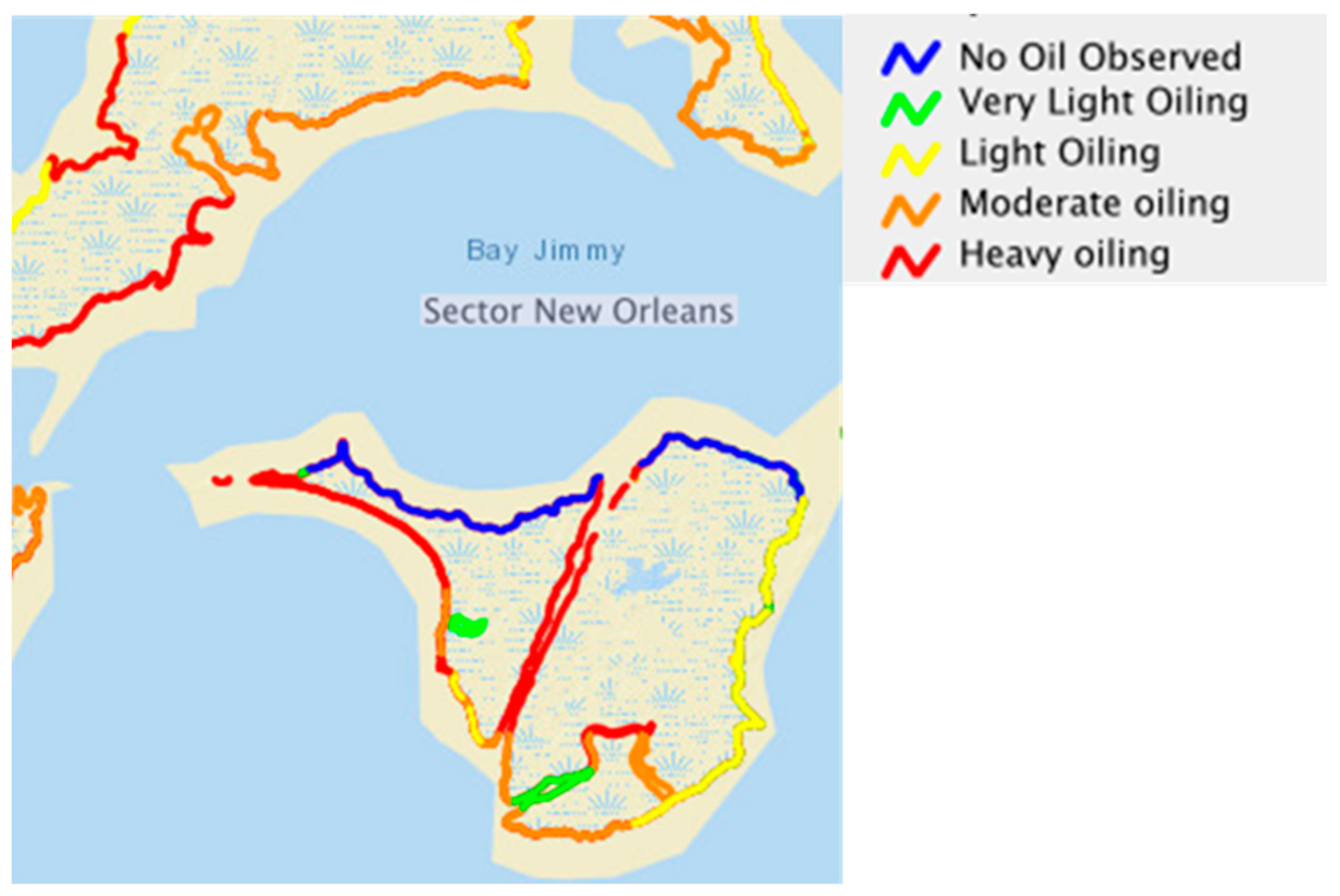[25] mapped the oil in the wetlands of Barataria Bay using the Multiple Endmember Spectral Mixture Analysis (MESMA) applied to a spectral subset of AVIRIS data obtained with a band selection algorithm. A spectral library was generated using spectra extracted from the hyperspectral image or acquired in the field. The method produced a detailed map of the oil spill, but as in the previous works, a set of possible endmembers had to be built beforehand.

The aim of this study was to develop strategies to detect very different cases of petroleum pollution: (i) oils mixed with soil or sand, (ii) oil deposited on shorelines, and (iii) tar pits. The methodologies developed in this work combine several detection methods, the aims being to achieve almost full automation and rely as little as possible on spectral libraries. Hydrocarbon indices developed in [18], were used to detect subtle HC absorption bands in noisy spectra, in the cases where these HC absorption bands were sufficiently discernible. Because there are generally very few oil-contaminated pixels in the images, the potential of anomaly detection methods was also assessed. Finally, the use of spectral unmixing to search for and map oiled materials was investigated. In this study, different approaches were combined in order to make the most of their respective advantages. For instance, anomaly detection looks for all types of atypical pixels in the image and hydrocarbon indices are used to detect hydrocarbon-bearing materials, but usually with false positives. By combining the two methods, the number of false positives was reduced. Similarly, HC indices were used in unmixing methods to select the endmembers of interest.

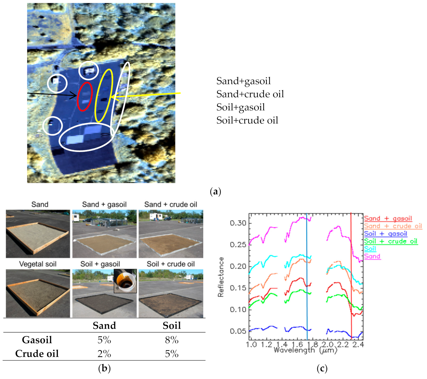
The methodology development and performance assessment of the different detection strategies were based on a proof of concept (POC) experiment that took place on the Fauga-Mauzac (France) site of ONERA, where boxes containing intimate mixtures of oil and soil or sand were set up.

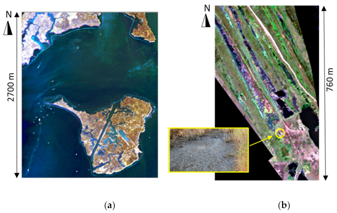
Two very different cases of real pollution were studied. The first was the coastal pollution caused by the DWH blowout in the Gulf of Mexico. In the second, the object of interest was a tar pit located on a former oil extraction site surrounded by vegetation.

2. Hyperspectral Images and Pre-Processing

2.1. POC Image

The hyperspectral images were acquired on 21 September 2015 using two HySpex cameras from NEO (Norsk Elektro Optikk)—a VNIR1600 and a SWIR320m—which have 160 spectral bands in the VNIR domain (0.4 μm–1.0 μm) and 256 bands in the SWIR domain (1.0 μm–2.5 μm), respectively. The cameras were installed onboard a Piper Aztec PA23-250 of SAFIRE (The French facility for airborne research). The ground sampling distance (GSD) is 0.5 m for the VNIR data and 1 m for the SWIR data. The radiometric correction, done using the NEO software, was followed by a correction of the aircraft window transmission. Calibration was also checked based on reference panels measured in-situ during the flight using an ASD FieldSpec spectroradiometer. Atmospheric compensation was performed using COCHISE (atmospheric COrrection Code for Hyperspectral Images of remote SEnsing sensors) software [28] which retrieves the surface spectral reflectance and water vapor content from the at-sensor radiance image, and also removes the atmospheric and the environmental effects. The atmospheric radiative parameters are computed using MODTRAN 5 [29]. The image was not geo-referenced.

Figure 1 shows an overview of the Fauga site and of the four 3 m × 3 m boxes of soil or sand mixed with gasoil or crude oil placed directly on the ground (asphalt). The crude oil is a Nigerian medium gravity oil. Its assay gives a proportion of 22% of paraffins, 44% of naphtenes, 34% of aromatics, and less than a percent of asphaltene (N-heptane insoluble). Mixtures were prepared using a concrete mixer to ensure homogeneity. Two boxes containing clean sand and soil were also set up. The sand was a non-homogeneous sand of coarse granularity. The soil was composed of clay, fine and coarse limestone, and fine and coarse sand.

The mean reflectance spectra of the six boxes extracted from the HySpex SWIR image are shown in Figure 1c. The HC spectral features in the 1.7-µm (blue vertical line) and the 2.3-µm (red vertical line) spectral areas are clearly visible in the mixtures with gasoil but much less so in the crude oil mixtures, particularly those with soil.

In order to quantify the results of spectral unmixing and anomaly detection, particularly in the case of subpixel detection, a synthetic image was built based on spectra extracted from the POC VNIR and SWIR images. In the case of the HC mixtures, the pixels at the center of the boxes were taken, and for each background material several spectra were extracted to take into account spectral variability. The distribution of materials is shown in Figure 2. The 3 × 3 small square pixels (the targets) are composed of a percentage x (x = 100, 75, 50, 25 from left to right) of HC mixed with soil or sand, and a percentage (100 − x, from left to right) of the corresponding background material (soil or sand). Targets containing mixtures with crude oil are positioned following a descending diagonal, while targets with gasoil follow an ascending diagonal. The first two rows and the last four rows of targets contain HC+sand mixtures, while the third to eighth rows of targets contain HC+soil mixtures. Out of the 102,400 pixels of the image, only 864 (less than 1%) contain an HC mixture. The background pixels are linear combinations of two of the three background material types (sand, soil, and various types of vegetation) with a continuous vertical variation from 0% to 100% abundance for the first and from 100% to 0% for the second, as shown in Figure 2. In order to add a cluttered area likely to generate false alarms in the detection process, patches of vegetation were included in the synthetic image. These patches were extracted from the HySpex VNIR and SWIR images, and registered using ENVI software and reference points.

2.2. Deep Water Horizon Image

The AVIRIS image, which can be downloaded on the NASA website [30], was acquired above Bay Jimmy, south of New Orleans between 29.252639°N, 89.907328°W and 29.588961°N, 89.859397°W on 14 September 2010. The instrument was mounted onboard a Twin Otter aircraft. Available images were geo-corrected with a spatial sampling of 3.5 m. The uploaded data are in radiance unit with 224 contiguous spectral bands from 400 to 2500 nm and a spectral sampling of 10 nm. In this work, part of this image, shown in Figure 3a, was processed. Atmospheric correction was performed using COCHISE.

2.3. Tar Pit Image

Hyperspectral images were acquired by the two HySpex cameras in June 2015 on a former oil exploration site in a tropical area in West Africa. The cameras were installed onboard a Flacon 20 of the French Aviation Defence Sevice. The pixel sizes of the VNIR image and the SWIR image were 0.65 m and 1.3 m across the track, and 1.3 m and 2.6 m along the track, respectively. The same radiometric calibration and atmospheric compensation method as for the POC image were applied. The two HySpex hypercubes were oversampled by 0.65 m by means of a nearest neighbor filter and coregistered using GeFolki [31], considering a SPOT 7 image as reference. The subset of 561 × 948 pixels used in this study is shown in Figure 3b. To focus on the area of interest and on the overlap region of VNIR and SWIR images which do not have the same field of view, a mask was built. Some pixels with an inconsistent spectral reflectance between VNIR and SWIR, due to the fact that the VNIR and SWIR cameras do not originally have the same GSD, were also masked out. The VNIR and SWIR bands of these spectra can exhibit a sharp discontinuity at around 1 µm. In order to limit the impact of these pixels on the image processing, those with a reflectance discontinuity greater than 0.1 were masked out. There ultimately remained 380,595 unmasked pixels.

3. Methodology Development

In this study, several approaches were applied, alone or in combination, to detect oil pollution. The first method made use of the specific spectral characteristics of hydrocarbons around 1.7 µm and 2.3 µm using the hydrocarbon indices defined in [18] which are less sensitive to noise than those based on a depth estimate of these absorption bands, such as the Kühn index:

$$KHI=\frac{{\lambda }_B-{\lambda }_A}{{\lambda }_C-{\lambda }_A}\left(R_C-R_A\right)+R_A-R_B$$

(1)

with $R_{A,B,C}$ being the reflectances at the wavelengths ${\lambda }_{A,B,C}$ where B is the center of the absorption band (~1.730 µm), whereas A and C are on the shoulders of the absorption band (~1.70 µm and ~1.74 nm).

Although they are generally effective for detecting oil pollution, the indices mentioned here cannot be used to identify the type or abundance of hydrocarbons. A second method, based on autonomous spectral unmixing, was evaluated as regards its capacity to discriminate between different hydrocarbon compounds and quantify them in terms of abundance in pixels. Finally, the benefits of anomaly detection methods were assessed, as in most cases of onshore oil spills, there are few impacted pixels in the image, and these constitute atypical pixels. Moreover, when hydrocarbons are biodegraded, they do not systematically present specific spectral features at 1.7 and 2.3 µm, and so cannot be reliably detected with the help of HC indices.

3.1. Spectral Indices

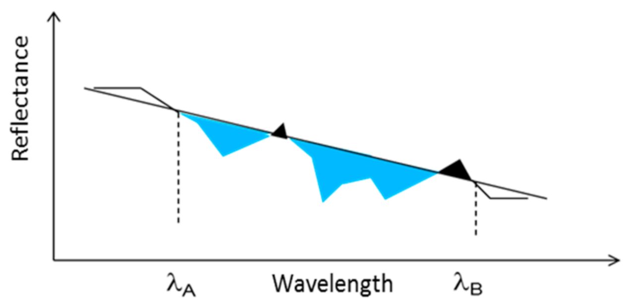
The hydrocarbon indices Area1700 and Area2300 [18] represent the area of the absorption bands under a virtual line drawn between λ_A = 1.66 and λ_B = 1.75 µm (Area1700) and λ_A = 2.21 and λ_B = 2.38 µm (Area2300) as illustrated in the Figure 4. The advantage of these indices is that they are less sensitive to noise and to the center position of the absorption bands, which varies according to the HC composition as shown by laboratory measurements [5]. The absorption band centers of aromatic HC are between 1.67 and 1.70 µm, while those of aliphatic HC are around 1.725 µm. Both aromatic and aliphatic HC have strong spectral features around 2.3 µm, and aromatic HC have spectral features at 2.14–2.18 µm.

3.2. Spectral Unmixing

The second method we developed was presented in [18]. It combines unmixing with spectral index calculation. The goal of unmixing methods is to identify pure materials in a hyperspectral image (the endmembers) and to estimate the related abundances in each pixel. A review of unmixing methods can be found in [32].

A commonly used assumption is that the different pure components (endmembers) are linearly mixed in the pixels, as it allows to model macroscopic mixing phenomena for flat surfaces. [33,34]. This assumption can be made because the objective is to search for the spectral signature of polluted soils and not to extract the spectra of pure HC into the mixture. Indeed, polluted soils are themselves intimate mixtures of HC and soil that cannot be modeled by a linear mixing model. Characterization of intimate mixtures does not fall within the scope of this study, but the reader can refer to the works of Schwartz et al. and Okparanma et al. for example [20,35].

The linear mixing model can be formulated as follows:

$$p_{ij} = {\displaystyle \sum }_{k=1,\mathrm{K}}{e}_{ik}{a}_{kj}+w_{ij} s.t.0\le a_{kj}\le 1\&{\displaystyle \sum }_{k=1,\mathrm{K}}{a}_{kj} = 1$$

(2)

where $p_{ij}$ is the radiance or reflectance of the pixel j in the band i, and $e_{ik}$ is the reflectance of the endmember k in the band i, $a_{kj}$. is the abundance of the endmember k in the pixel j, and $w_{ij}$ is an additive perturbation (e.g., noise and modeling errors). K is the total number of endmembers.

In this work, a method based on the Orthogonal Subspace Projection (OSP) was used to extract the endmembers [36]. We chose the OSP method because the algorithm is deterministic (it contains no random draw) and therefore its results are reproducible. In addition, it is unnecessary to set an a priori number of endmembers in the image, a tricky issue that has a significant impact on results in most endmember extraction methods. This number can be estimated using methods such as HYSIME [37] or HFC [38], but they produce results that vary according to the image noise and the spectral variability of the materials present in the image. The principle of the OSP method is to search iteratively for extrema pixels. At each iteration, data are projected orthogonally onto the subspace supported by the endmembers (extrema pixels) previously extracted and a new search is run to find the next endmember. Therefore, increasing the number of endmembers makes no change to the endmembers already extracted with a smaller value of K. After the endmembers have been extracted, abundance maps of each endmember are computed using the FCLS (Fully Constrained Least Squares) method [39].

The next stage consisted in finding the endmembers of interest, i.e., those corresponding to the oil-impacted materials. For this purpose, the endmembers were sorted in descending order according to their Area1700 score. Area2300 was also computed.

The possibility of distinguishing different types of HC compounds—which is impossible using only the spectral indices mentioned above—and of mapping the endmembers of interest, was evaluated using this method.

3.3. Anomaly Detection

Anomaly detection methods are interesting for detecting HC whose spectral signatures have no or poorly detectable specific spectral characteristics. However, they can also be used in combination with spectral index calculation to reduce the number of false alarms.

Before the actual detection process, a PCA (Principal Component Analysis) transform was applied to the image in order to reduce the spectral dimension. The number of principal components (PC) to be retained was computed using the Growing Ratio method [40], but the minimum number of PC was set to 8. Consequently, the number of PC considered in the detection was equal to the maximum value between 8 and GR, GR being the number of significant PC estimated using the Growing Ratio method.

Many types of anomaly detectors (ADs) have been proposed in the literature [41,42,43]. The most frequently used is the Reed–Xiaoli (RX) detector [44] that often serves as a benchmark for other methods. RX derived methods have been widely used, are easy to implement, and their performance has been assessed on many cases, which is why we chose them for this work. The RX detector characterizes the background by its spectral mean ${\overrightarrow{\mu }}_B$, ${\overrightarrow{\mu }}_B$ being a column vector of size N, the spectral dimension, and its spectral covariance matrix ${\sum }_B$ of size NxN. The detector calculates the Mahalanobis distance between the pixel under test $\overrightarrow{p}$ (column vector of size N) and the background. ${\overrightarrow{\mu }}_B$ and ${\sum }_B$ can be calculated on the entire image (Global RX) either in a sliding window around the pixel under test (Local RX or LRX) or on clusters after a clustering step. In this work, we used LRX and a Class-conditional version of RX (CRX) [43].

In the CRX method we have developed, the clustering step is performed using a K-means algorithm based on Euclidian distance. Five runs of K-means were performed and the result with the smallest intra-class inertia was kept. A maximum number of classes was set, as well as a minimum number of pixels per class to prevent the anomalies from constituting their own class. In the CRX method the covariance matrix and mean spectrum within each class i (i.e., ${\sum }_{B,i}$ and ${\mu }_{B,i }$) are calculated, followed by the Mahalanobis distance between $\overrightarrow{p}$, the pixel under test (PUT), and each of the classes. The anomaly score is the minimum of these distances:

$$D_{CRX}\left(\overrightarrow{p}\right)=\underset{i}{\min }\left[{\left(\overrightarrow{p}-{\overrightarrow{\mu }}_{B,i}\right)}^t{\sum }_{B,i}^{-1}\left(\overrightarrow{p}-{\overrightarrow{\mu }}_{B,i}\right)\right]$$

(3)

In the LRX method, the covariance matrix and mean spectrum of the background are estimated locally using a triple window centered on the PUT. In our implementation of the method, the size of the guard window, W_g, (set to avoid contamination of the background statistics by the PUT) is a parameter based on which the sizes of the other two windows W_µ and W_∑ are determined according to the number of variables, n, (spectral bands or principal components) that describe the data:

$$W_{\mu }=mi{n}_{kodd}\left(k^2-W_g{}^2\ge \sqrt{10n}\right)$$

(4)

$$W_{\Sigma }=mi{n}_{kodd}\left(k^2-W_g{}^2\ge 10n\right)$$

(5)

These parameters make it possible to estimate the covariance matrix and the mean spectrum of the background as locally as possible, while ensuring a sufficient number of samples for estimating the statistical parameters. The anomaly score is then defined by

$$D_{LRX}\left(\overrightarrow{p}\right)={\left(\overrightarrow{p}-{\overrightarrow{\mu }}_{W_{\mu }}\right)}^t{\sum }_{W_{\sum }}^{-1}\left(\overrightarrow{p}-{\overrightarrow{\mu }}_{W_{\mu }}\right)$$

(6)

${\overrightarrow{\mu }}_{W_{\mu }}$ being the mean spectrum computed in the window of size W_μ, and ∑_W∑ being the covariance matrix computed in the window of size W_∑.

The pixel under test $\overrightarrow{p}$ is an anomaly if $D_{CRX}\left(\overrightarrow{p}\right)>\eta$ (or $D_{CRX}\left(\overrightarrow{p}\right)>\eta )$, $\eta$ being the detection threshold to be set by the user. For instance, it can be set to detect 1/100 of the pixels in the image (i.e., the 1% most atypical pixels). One can also visualize the anomalies with the highest values of $\eta$ to focus on the first detections.

3.4. Performance Evaluation

Detection

To quantitatively evaluate the detection results, the ROC curves (Receiver Operating Characteristic)—i.e., the detection rate vs the false alarm rate—can be computed if the target location is known. In this case, target masks were built and used to count true and false detections (false alarms). The false alarm rate is shown on a logarithmic scale in order to place the emphasis on low false-alarm rate values. The area under the curve, hereafter known as LogAUC, was computed with the false-alarm rate in logarithmic scale, to obtain a global detection performance criterion.

Spectral Unmixing

To evaluate the accuracy of the endmembers, the spectral angle and the root mean square error (RMSE) between the true spectra and the extracted endmembers were computed. The spectral angle, written SAM in the following, is defined as

$$SAM\left(\overrightarrow{x},\overrightarrow{y}\right)=arccos\left(\frac{\langle \overrightarrow{x}.\overrightarrow{y}\rangle }{\Vert \overrightarrow{x}\Vert \Vert \overrightarrow{y}\Vert }\right)$$

(7)

where $\overrightarrow{x}$ and $\overrightarrow{y}$ are two spectra (column vectors of size N), 〈 〉 is the scalar product and ‖ ‖ is the Euclidian norm. The spectral angle measures the similarity of shapes between spectra. It was also used to pair the endmembers extracted with the pure material spectra of the image.

The RMSE is computed as follows:

$$RMSE\left(\overrightarrow{x},\overrightarrow{\hat{x}}\right)=\frac{\Vert \overrightarrow{x}-\overrightarrow{\hat{x}}\Vert }{\Vert \overrightarrow{x}\Vert }$$

(8)

where $\overrightarrow{\hat{x}}$ is an estimate of $\overrightarrow{x}$.

The reconstruction error is used to evaluate the accuracy of the unmixing. It is the difference between the actual value of a pixel and its estimated value based on the endmembers and their abundance in the pixel. Using the notation of Equation (2), it is written:

$$E{R}_j=\frac{\sqrt{{\sum }_{i=1,B}{\left(p_{ij}-e_{ik}{a}_{kj}\right)}^2}}{\sqrt{{\sum }_{i=1,B}{p}_{ij}{}^2}}\times 100$$

(9)

4. Application to the Controlled Experiment

The methodologies developed were first tested on data acquired during the POC campaign, on the image itself and on a synthetic image built from the former, in order to quantify and compare the performances of the three different approaches studied.

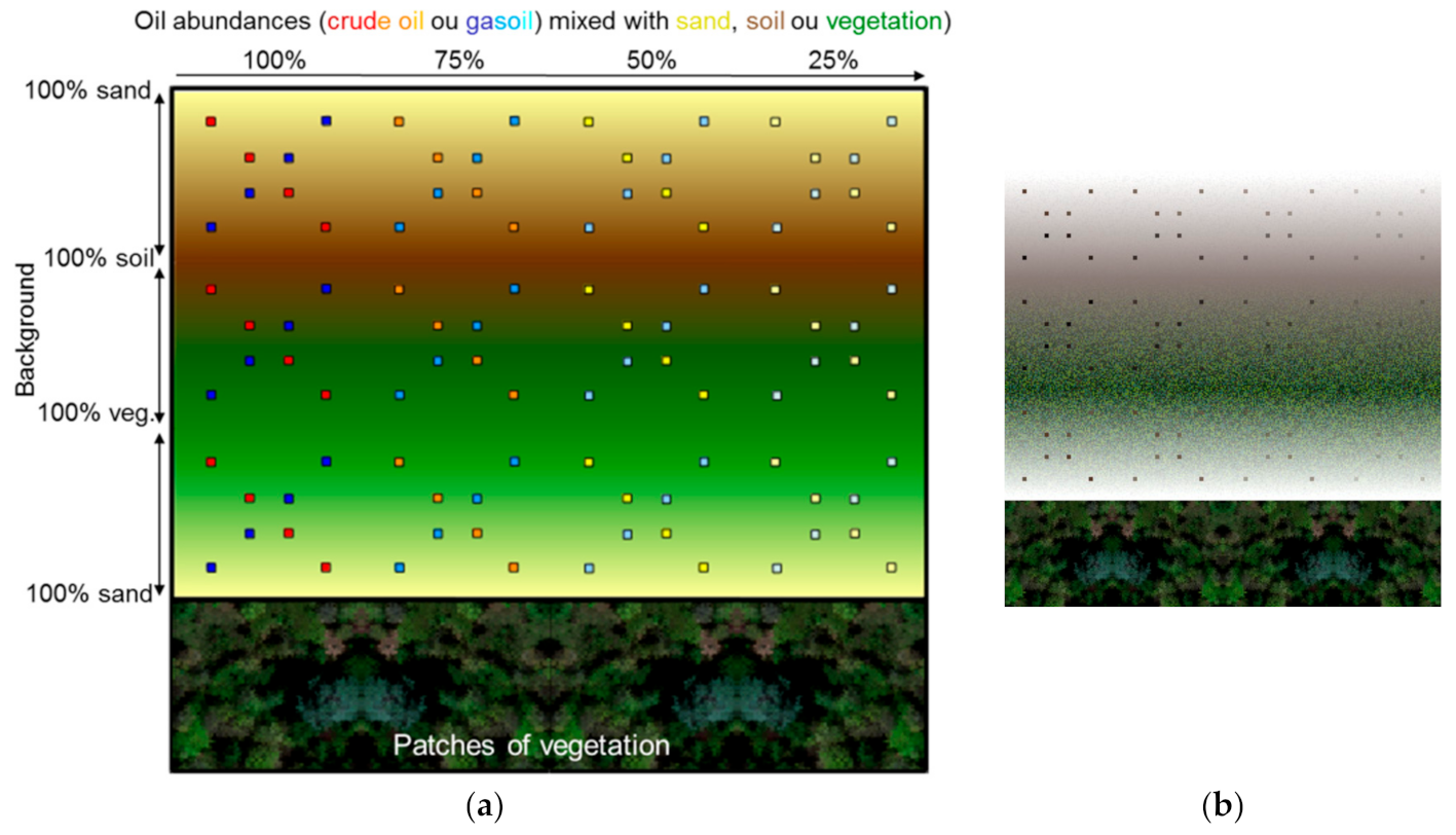
4.1. Application to the POC Synthetic Image

Anomaly detection was first assessed on the synthetic image. Target masks for each mixture were built to evaluate the detection rate versus false-alarm rate. First, a PCA transform was applied to the image in order to reduce spectral dimension. Eight principal components were retained. With LRX, the guard window was set to 5 × 5 or 11 × 11 pixels to assess the impact of this parameter. With CRX, the maximum number of clusters was set to 20, 30, or 40, and the minimum numbers of pixels per class was set to 200.

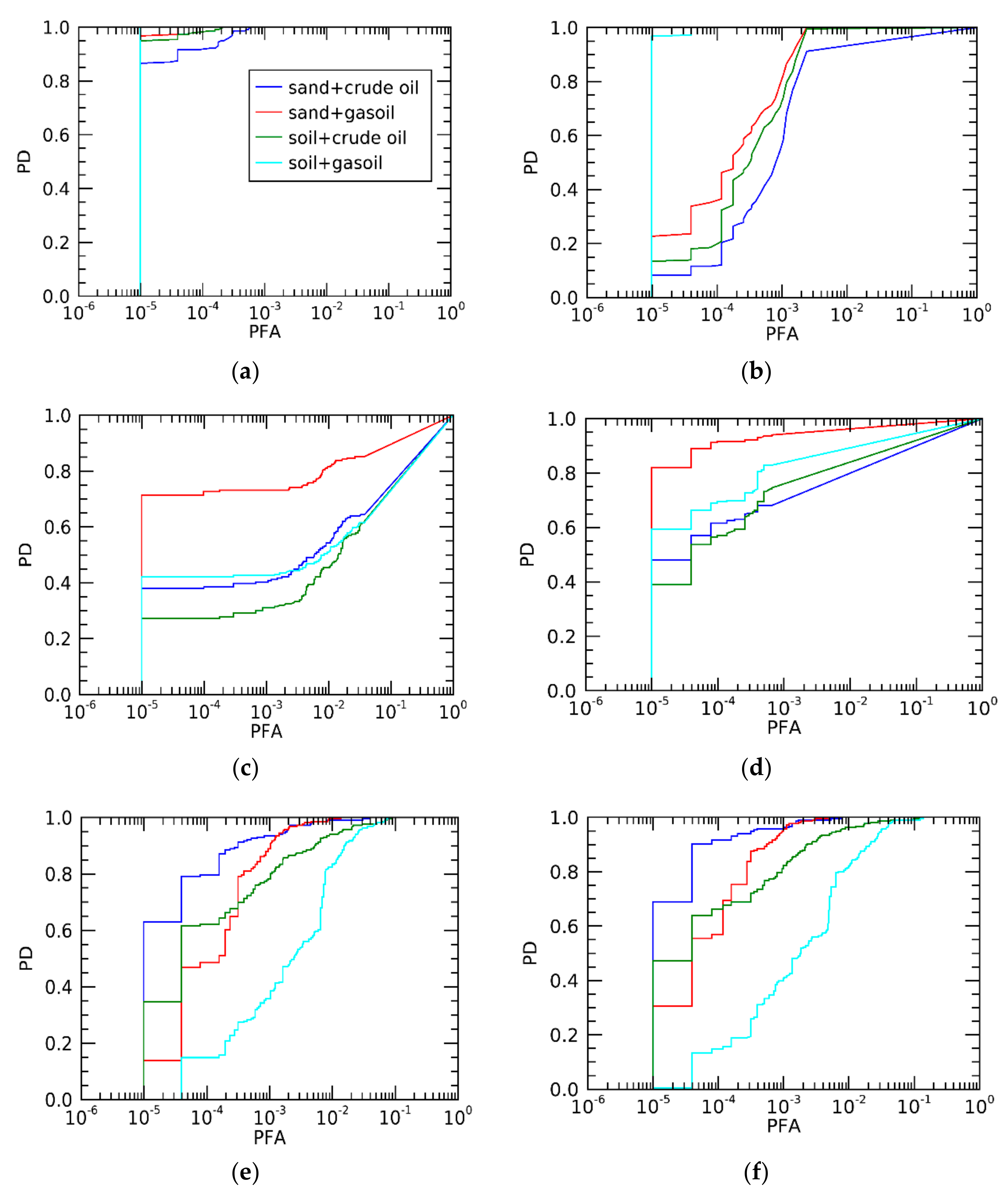
The ROC curves are shown in Figure 5 and the LogAUC are given in

Table 1. LogAUC obtained with the different detection methods, anomaly detection LRX, CRX, and hydrocarbon indices calculations: Area1700, Area2300, and Kühn index (KHI). The last line corresponds to Area1700 applied to the most atypical 1% of pixels. The size of $W_g$ for LRX and the maximum number of classes for CRX are given in brackets.

	Sand Crude Oil	Sand Gasoil	Soil Crude Oil	Soil Gasoil
Anomaly detection
LRX (5)	0.97	1.0	0.99	1.0
LRX (11)	0.64	0.77	0.72	1.0
CRX (40)	0.94	0.84	0.83	0.57
CRX (30)	0.91	0.79	0.80	0.56
CRX (20)	0.79	0.68	0.59	0.45
Spectral indices
Area1700	0.55	0.80	0.48	0.56
Area2300	0.36	0.57	0.22	0.22
KHI	0.26	0.73	0.22	0.35
LRX(11)(1%) + Area1700	0.74	0.94	0.75	0.83

. As the false-alarm rate is displayed on a logarithmic scale, its minimum value was set to 1/102,400 (102,400 being the total number of pixels). The Figure 5 shows that all the first detections correspond to the targets except for soil+gasoil using CRX method.

The values of LogAUC for LRX with $W_g$ = 5, are equal or very close to 1 (perfect detector) for all the targets, the worst result being for sand+crude oil with a LogAUC value of 0.97. LRX performance decreases (up to 0.64) with a guard window equal to 11 because ${\overrightarrow{\mu }}_{W_{\mu }}$ and ${\sum }_{W_{\sum }}$ are not computed in close vicinity to the targets. CRX gives satisfactory results but requires a large number of classes in the clustering step. The best result is obtained with 40 clusters. The LogAUC values are higher than 0.8, except for the soil+gasoil mixture where they drop to 0.57. Performance decreases slightly with 30 clusters and significantly with 20 clusters. The reflectance of soil+gasoil mixture is very low and shows a high contrast with the pixels in its vicinity, which explains its perfect detection using the LRX. However, the low contrast with shaded areas certainly explains the poor detection performance obtained with the CRX method. “Soil + gasoil” pixel spectra is too close from shadow spectra present in the whole image.

Although anomaly detection succeeded in detecting pixels containing HC-based mixtures because they are atypical pixels in the image, there was however no evidence to confirm that they were oil-contaminated pixels. A spectral analysis was therefore required. On the simulated image, several spectral HC indices were tested, the Kühn’s index and the indices Area1700 and Area2300 we defined in [18]. Vegetation generated a large number of false alarms, especially the dry vegetation patch at the bottom of the image. To fix this issue, vegetation was suppressed using an NDVI (Normalized Difference Vegetation Index) test prior to computing the HC indices. An NDVI threshold of 0.3 was set to detect vegetation. Satisfactory results were obtained after vegetation rejection, even though mixed pixels composed of vegetation/HC mixtures with a high proportion of vegetation were suppressed. The corresponding ROC curves and LogAUC values are given in Table 1. The LogAUC of Area1700 is higher than that of the Kühn index (hereafter referred to as KHI), and also higher than that of Area2300, except in the case of soil+crude oil. All the spectral indices have significantly lower LogAUC than LRX and CRX but have the advantage of tagging the pixels detected as hydrocarbon compounds. Finally, anomaly detection and Area1700 were combined: Area1700 was computed on the most atypical 1% of pixels obtained with LRX11. The detection rate is better than the one obtained using one of the two methods on its own for three of the four mixtures. For instance, LogAUC values are 0.64 and 0.55 for LRX11 and Area1700, respectively, and it increases to 0.74 when the methods are combined. Moreover, the likelihood of the anomalies being oil-contaminated pixels is increased.

One can see on the ROC curves of all the anomaly detection methods that the false-alarm rate at the first detection is equal to its minimum value (1/102,400) which means that the first anomalies detected are pixels containing the HC mixtures.

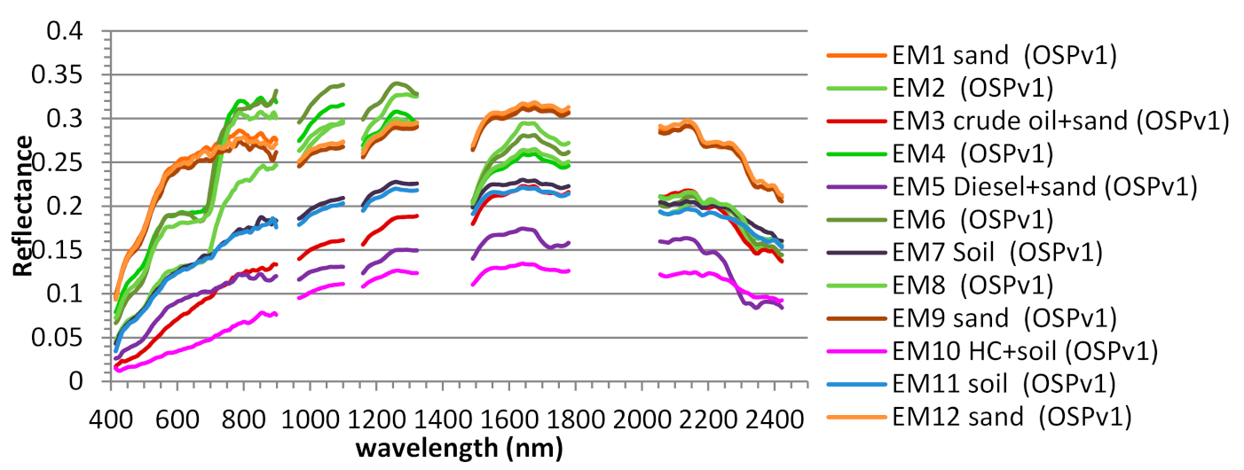
The unmixing method was also tested on the synthetic image. The objective was to extract the spectral signatures of the HC-substrate mixtures, but not to extract the pure HC signatures, which is a subject for the study of intimate mixtures. The method was first applied to the entire image, with the number of endmembers set to 15 after the vegetation was suppressed using the NDVI, in order to avoid endmember extraction in the vegetation patches (test called OSPv2). Indeed, vegetation (green and dry) presents a great spectral variability, which does not fall within the scope of this work. Moreover, the spectra resulting from the concatenation of VNIR and SWIR pixels, which do not have the same spatial resolution, may be inconsistent in some cases. In a second test (called OSPv1), the lower part of the image was removed in order to avoid this problem while preserving all pixels containing HC-based mixtures, even with a vegetation background. No vegetation rejection was performed on the rest of the image. The number of endmembers was set to 12.

In both cases, Area1700 was computed on all the endmembers (see

Table 2. Area1700 endmember values (values of the remaining endmembers are equal to 0), spectral angle values between each component and the closest endmember (considering spectral angle), and the corresponding RMSE. OSPv1: OSP applied to the entire image after vegetation rejection.

	Endmember	Area1700	SAM (°)	RMSE
Crude oil+soil	EM10	0.045	0.031	0.006
Gasoil+soil	EM10	0.045	0.113	0.048
Crude oil+sand	EM3	0.003	0.015	0.004
Gasoil+sand	EM5	0.347	0.014	0.002
Soil	EM12	0	0.011	0.004
Sand	EM11	0	0.011	0.003
Vegetation mixture	EM6	0	0.334	0.084

and

Table 3. Area1700 values of endmembers (values of the remaining endmembers are equal to 0), spectral angle values between each component and the closest endmember (considering spectral angle), and the corresponding RMSE. Case OPSv1: OSP applied to the image where the bottom part of the image showing vegetation has been removed, but without vegetation rejection test.

	Endmember	Area1700	SAM (°)	RMSE
Crude oil+soil	EM12	0.027	0.035	0.006
Gasoil+soil	EM12	0.027	0.086	0.058
Crude oil+sand	EM4	0.045	0.015	0.004
Gasoil+sand	EM7	0.337	0.014	0.002
Soil	EM11	0	0.011	0.003
Sand	EM1	0	0.012	0.004
Vegetation	EM9	0	0.039	0.009

) in order to identify those of the HC mixtures. Each mean spectrum of the background materials and HC mixtures (the four HC mixtures, soil, sand, and vegetation) was paired with the endmember with which it formed the smallest spectral angle. The Figure 6 shows all the endmembers extracted with OPSv1. Four endmembers (in green) with vegetation features are extracted, three endmembers are paired with sand spectrum, two endmembers, with soil spectrum and three endmembers with HC mixtures. The RMSE of each pair thus constituted was also computed. Spectral angles and RMSE are shown in Table 2 and Table 3. In both cases, the endmembers of crude oil or gasoil mixed with sand were easily extracted as indicated by Table 2 and Table 3, and as shown in Figure 7, but only one endmember, closer to the soil+crude oil spectrum than to the soil+gasoil spectrum, was retrieved in the case of the soil-based mixtures. This can be explained by the fact that the two spectra of soil-based mixtures have fairly similar shapes but have different reflectance levels. Consequently, when looking for extrema in the spectral space, the spectrum with the lowest level was not detected as being an extremum. The spectral angles between the endmembers and the associated mean spectra of the materials are very small (less than 1°) because the endmembers correspond to the spectra of these materials and differ from their mean only because of the spectral variability of the materials. The RMSE are also small for the same reasons, except in the case of the sand+gasoil mixture because the reflectance level of the associated endmember is higher than that of its mean spectrum.

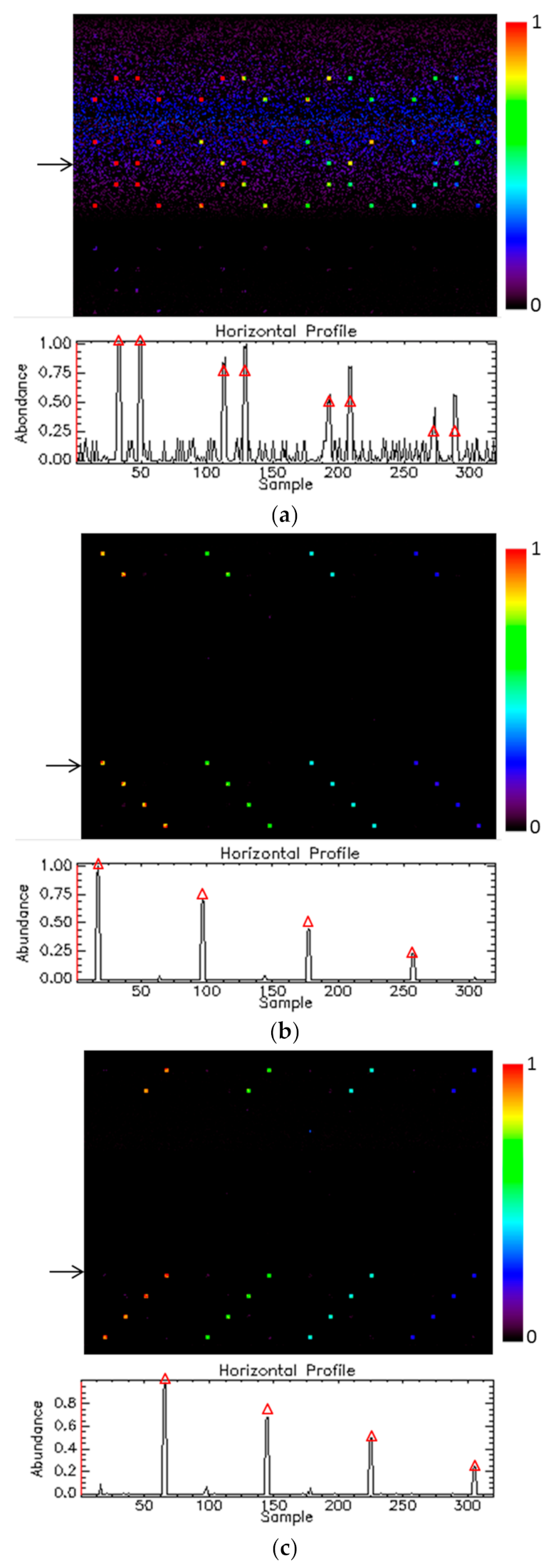
The abundance maps are shown in Figure 8 as is a horizontal profile of the abundance values for the case OSP2. For the sand+HC mixtures, the abundance map values, and the real abundance values are very close. However, for the soil+HC mixture, even though the maximum values are effectively located on the pixels containing the mixtures, residual values are also present in pixels without HC, and the abundance values of soil+gasoil are too high. Figure 9 shows the reconstruction error image. The error is very low across the entire image, except on pixels that contain the soil+gasoil mixture, where it can reach almost 100% because both the endmember level and the abundance value obtained on those pixels (to satisfy the sum to one constraint) are too high. Similar observations and tendencies were found in OSP1, so they are not mentioned in this paper.

4.2. Application to the POC Image

Anomaly detection and spectral index computation were applied to the SWIR HySpex image. The choice was made to focus the study on the SWIR image only in order to avoid the issues posed by the limited registration accuracy between VNIR and SWIR images, which also have different spatial resolutions. In particular, misregistration can cause artificial anomalies. The unmixing method was not applied to this image because the area where the experiments were conducted contained many objects, a lot of them made of plastic, which would have generated a very large number of endmembers.

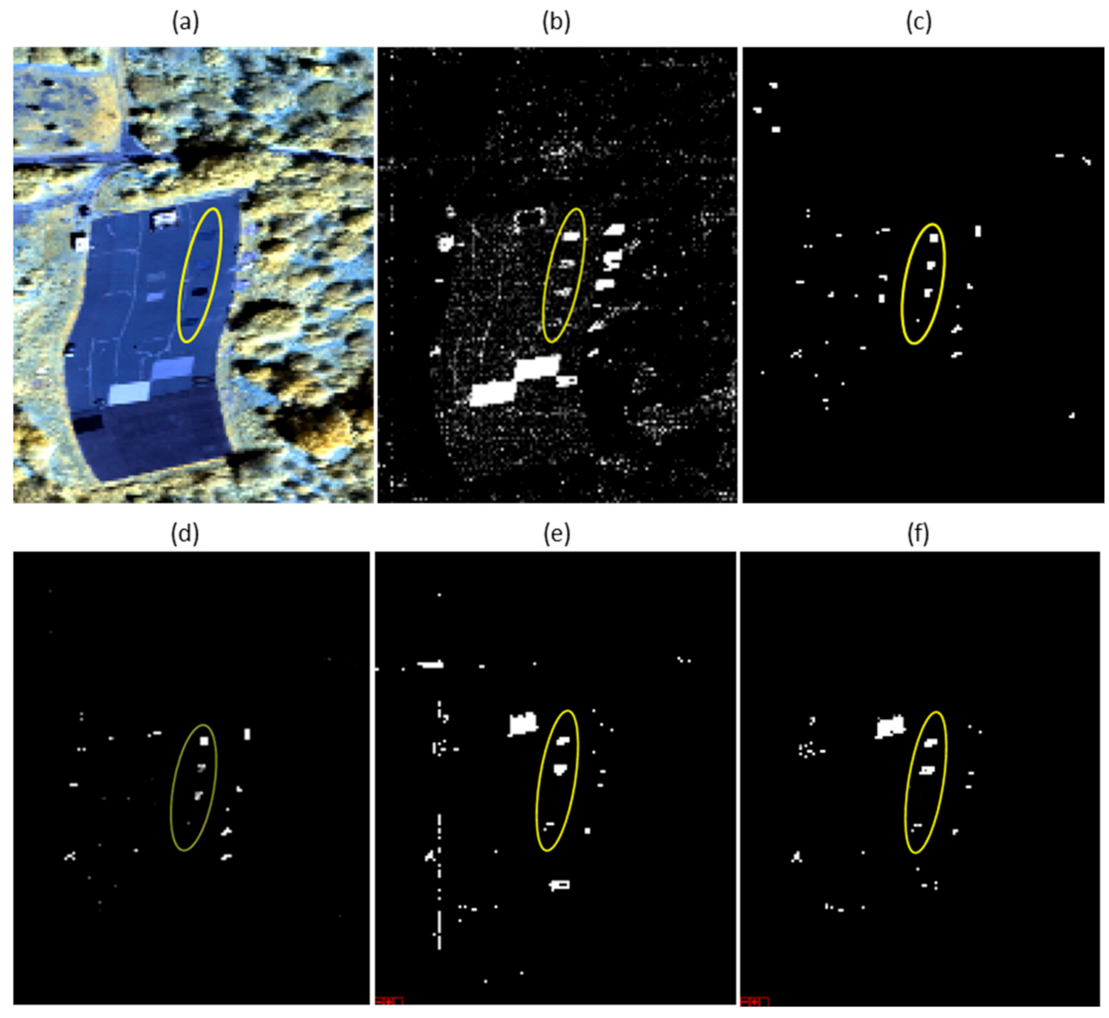
The results of anomaly detection and spectral index computation are illustrated in Figure 10. It shows the Area1700 scores (b) (arbitrary threshold), the pixels detected by LRX (c) and CRX (e) with a detection threshold of 0.01%, and the combination of both results: anomaly detection using LRX or CRX followed by Area1700 computation in (d) and (f), respectively. To avoid too many false detections on vegetation, especially dry vegetation, the NDNI (Normalized Difference Nitrogen Index) was computed and pixels with NDNI values greater than 0.1 were masked. The detection maps obtained with CRX and LRX differ: using the local detector, large plastic targets are undetected, and this is also true with CRX in the case of the largest targets as they are big enough to form a class. A vertical line corresponding to a defect on the detector array is detected with CRX.

All the methods were successful in detecting the two HC+sand mixtures. LRX detected the four mixtures—only one pixel on the soil+crude oil mixture—but with false alarms, located mainly in the vegetation shadow. CRX detected the mixtures except the soil+gasoil one, with false alarms that were different from those of LRX. The combination of anomaly detection and Area1700 reduced the number of false positives, and LRX combined with Area1700 produced the best results: three of the four mixtures were detected, and the other pixels detected were plastics.

5. Application to DWH

Part of the results shown in this section were presented in [19], but this paper gives a more detailed analysis.

5.1. Automatic Mapping Based on Hydrocarbon Indices

The hydrocarbon indices Area1700, Area2300, and KHI were computed on the image as shown in Figure 11. Area1700 and Area2300 make it possible to map the oiled shorelines, and also detect materials containing plastic components, such as boats and buoys that were deployed to prevent oil from reaching the coast. The detection maps obtained with Area1700 or Area2300 are in good agreement with results of previous works carried out in the same area on the same day [15] and shown in Figure 12. The two maps are also quite similar to the one featuring the most impacted soils in red and orange shown in Figure 13 drawn from ground observations three days after the AVIRIS image collection, on September 17, available on the Environmental Response Management Application (ERMA) website [45]. Some false alarms are present on the in-land vegetation patches, particularly on the Area2300 map. The Kühn index, shown in Figure 13c, detects some of the oiled shorelines, but throws up many false detections on the unpolluted coasts and inland. Moreover, it appears to be very sensitive to instrument noise. In particular, artifacts composed of regular spatial features are visible on the map.

5.2. Automatic Mapping with Endmember Extraction

In order to refine the mapping of oiled shorelines, the unmixing method was applied to the same AVIRIS image.

In order to avoid the detection of numerous undesirable elements during the endmember extraction process, a mask was applied to the boats and the plastic buoys around the islands. In the OSP unmixing method, the number of endmembers was set to 20. Endmember extraction was applied to a spectral subset containing the two main HC spectral features at 1.7 and 2.3 µm: the spectral ranges from 1.5923 µm to 1.8015 µm and from 1.9674 µm to 2.4962 µm. The next stage consisted in finding the endmembers (referred to as EM in the following) of interest, i.e., those corresponding to the oiled materials. To do so, EMs were sorted in descending order according to their HI, Area1700 and Area2300 scores. For greater clarity, hydrocarbon indices were normalized.

Table 4. Endmembers sorted according to their Area1700 index normalized between 0 and 1 (values in parenthesis). Normalized values of Area2300 are also shown.

	Area1700	Area2300
1	EM3 (1.000)	EM3 (1.000)
2	EM14 (0.665)	EM5 (0.680)
3	EM5 (0.487)	EM17 (0.517)

presents the EM sorted according to their HC indices (their values are given in parentheses). Figure 14 shows the spectra across the entire spectral range for EMs 3, 5, 14, and 17, and Figure 15 shows their abundance maps. The absorption bands at 1.72 and 2.3 µm are clearly visible on the spectra. The spectra of the 3rd, 14th, and 17th EM correspond to oiled vegetation, as measured in the field or the laboratory [15]. The 3rd and the 17th delineate the same area, but the pixels with the highest values for the 3rd and the 17th EM are not superimposed: in most cases, the highest values of the 17th EM are closer to the water and those of the 3rd are right behind. The 17th EM corresponds to a heavily oiled marsh [15], which is consistent with the location of the highest abundance values, near the water. The 3rd EM likely represents a marsh area that is somewhat less heavily affected by the oil, which is also consistent with the location of its highest abundance values. The 14th EM corresponds to oiled green vegetation. Its maximum abundance values are also found near the water.

The abundance maps of the 3rd, 14th, and 17th endmembers define the oiled shorelines. When comparing them with Figure 12 and Figure 13, the oiled areas detected are similar to those obtained by Kokaly [15], and with the highly and moderately oiled areas observed in the field three days after the event [45]. The maximum abundance values of the 5th endmember are near the shoreline, with significant values for two pixels only, and very low values elsewhere. Its spectrum, shown in Figure 14, most likely corresponds to a boat or a plastic object.

Compared to spectral index calculations, the unmixing strategy makes a finer analysis of the oiled shoreline possible, as it helps to distinguish several areas more or less impacted by the spill, while remaining nearly fully automated and without any need for spectral libraries.

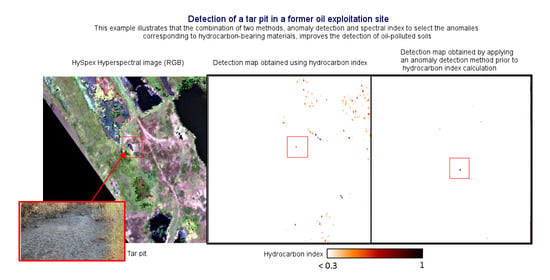
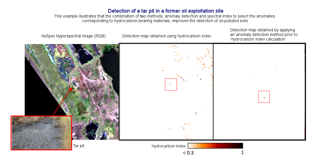
6. Tar Pit Detection

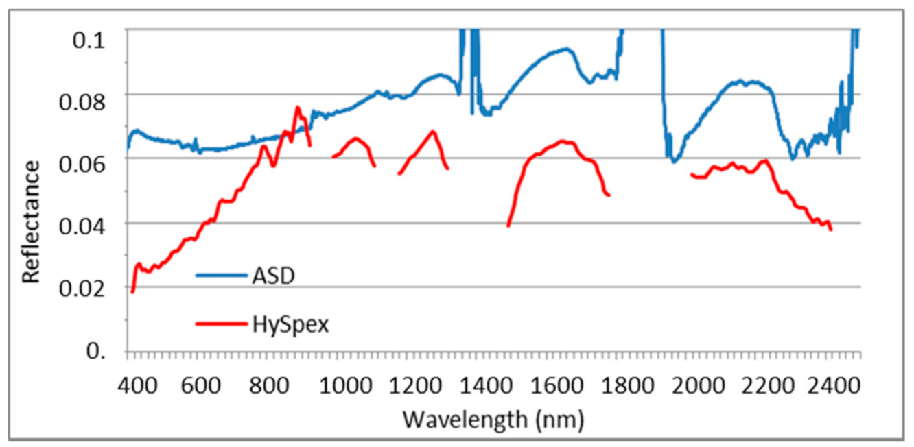
The tar taken from the pit was measured in the laboratory using an ASD FieldSpec spectroradiometer. Its spectral reflectance is shown in Figure 16 together with the spectrum acquired with the HySpex cameras. The HC 1.7 µm spectral feature of the tar is clearly visible on the ASD spectrum as well as a sharp decrease of the reflectance after 2.3 µm. On the HySpex spectrum, the large atmospheric water vapor absorption band, brought about by the high humidity levels in tropical areas, masks part of the 1.7 µm feature on the HySpex spectrum and the 2.3 µm spectral feature is less pronounced. The two instruments have a low signal-to-noise ratio at these wavelengths, which may partly explain this difference. Moreover, HC absorption is weaker on the spectrum acquired with HySpex because it corresponds to tar taken from the surface of the pit, which is crusty and likely more biodegraded than the tar measured in the laboratory, which was extracted from beneath the surface.

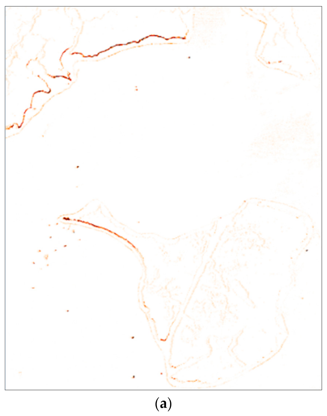
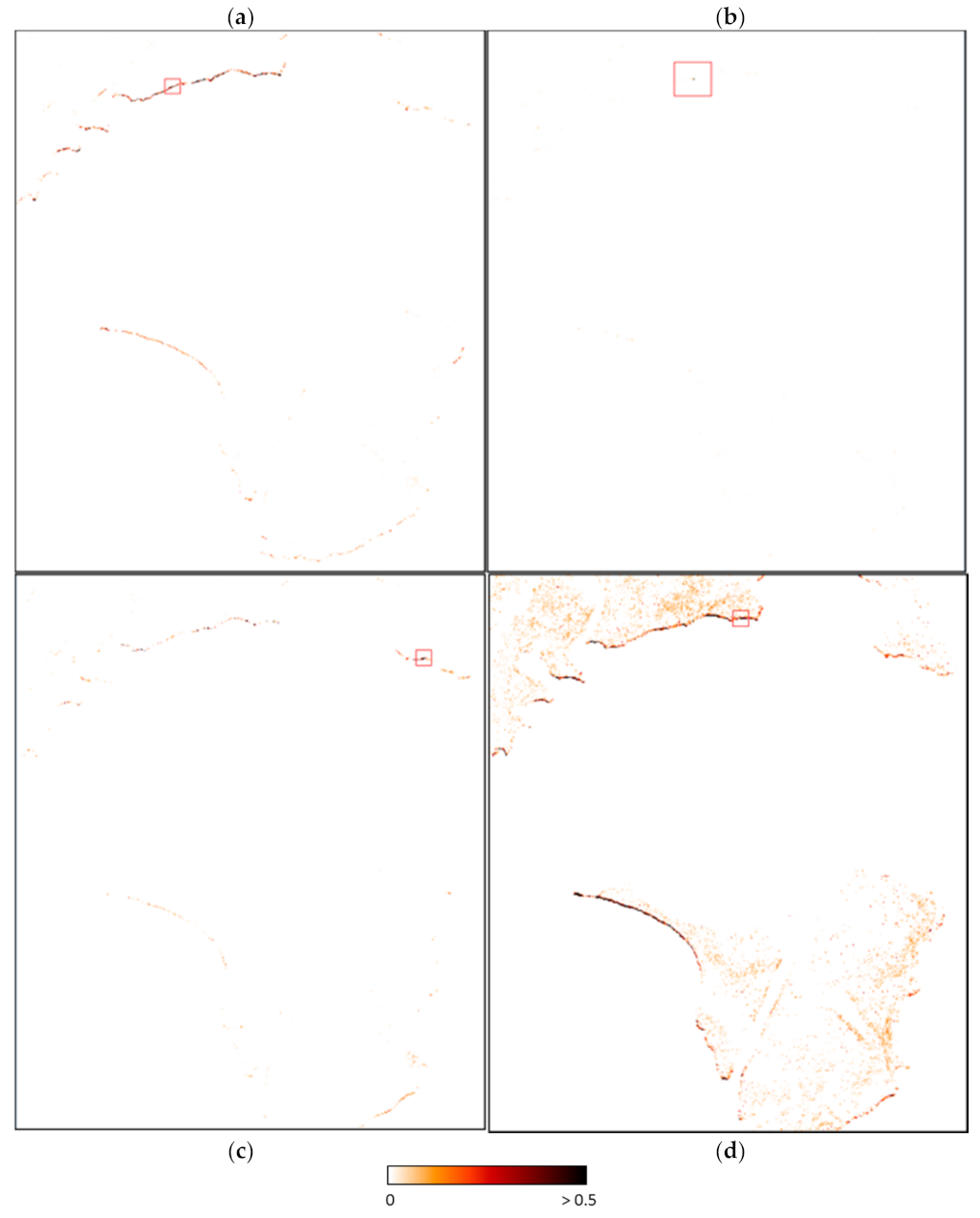
On the HySpex hypercube, the HC features are visible only at the center of the pit, which corresponds to one pixel at the GSD of the SWIR image. After resampling to 0.65 m and registration, the reflectance spectrum was duplicated as five pixels using the “nearest neighbor” resampling option. This choice was made in order to preserve the spectral shape, but it presents the disadvantage of making the objects appear deformed. Spectral indices KHI, area1700 and Area2300 were computed, but they generated many false alarms, especially on lagoons. To take into account the broad water vapor absorption band, the upper bound wavelengths of Area1700 and KHI were modified to 1.74 µm, and the center wavelength for KHI was set to 1.702 µm. The best result, obtained with Area1700, is shown in Figure 17, but many false alarms are still present on lagoons.

Because tar pits are rare, they are atypical and could be highlighted using anomaly detection. Some prior knowledge about the pit was considered. First, tar pits have a low reflectance in the 0.4–2.5-µm spectral range. So, anomalies with a reflectance value greater than 0.1 at 1.25 µm were excluded. Second, an NDVI test with a threshold of 0.3 was applied in order to mask vegetation pixels. At the end of these tests, which were carried out during post-processing, i.e., after the anomaly detector was applied, the only elements remaining on the image, in addition to the tar pit, were the lagoons of different depths, the mud surrounding them, composed mainly of organic matter, and other dark pixels.

LRX and CRX were applied to the image. LRX did not produce satisfying detection results because many of the elements in the image were the same size as the tar pit itself. This led to many false detections, as shown in Figure 18. CRX did not sustain this problem because elements of the same nature were grouped into clusters (results obtained with CRX were already presented in [46]). In order to evaluate the detection, two target masks were built, one to count the true positives, and the other to exclude pixels at the edge of the tar pit that could be a mixture of background material and tar. 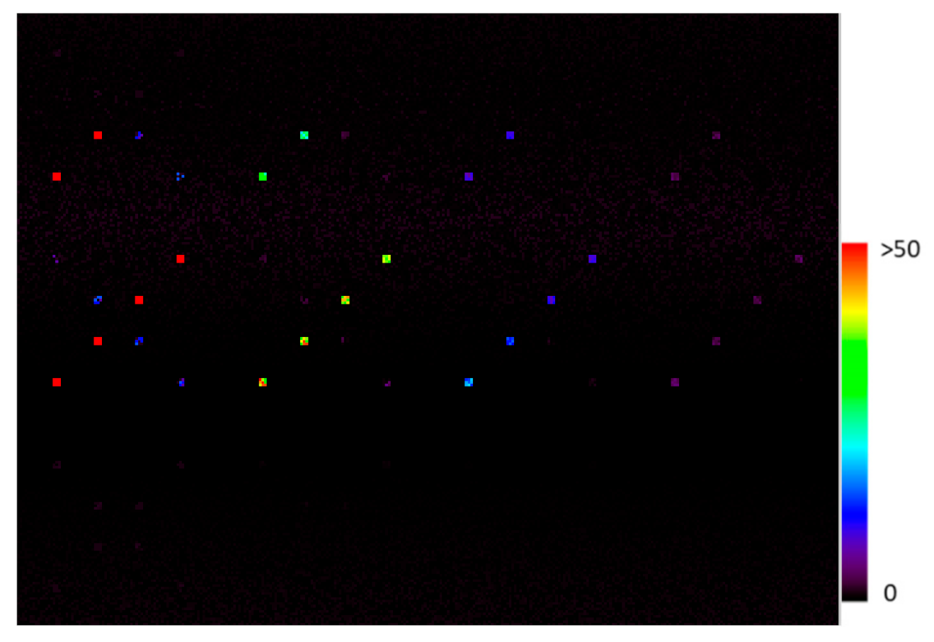Figure 18 shows the image of the RX score. The false-alarm rate for the first detection was 2.63 × 10⁻⁶. It corresponds to only one pixel, whose spectrum is non-physical but was not rejected by the spectral consistency test because the reflectance discontinuity between the VNIR and SWIR ranges is about 0.06, which is lower than the test threshold.

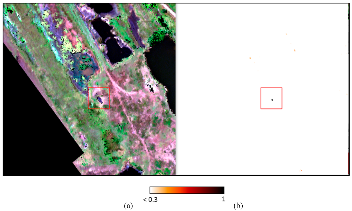
Spectral index computation and anomaly detection were then combined. First, CRX was applied, and the threshold was set to select one thousandth of the most atypical pixels. Area1700 was run on the pixels selected. The only pixel detected was at the center of the tar as shown in Figure 19. This result once again illustrates the benefit of combining two different detection strategies.

7. Discussion

7.1. Anomaly Detection Combined with Spectral Indices

In cases where the spectral features of hydrocarbons are clearly identifiable on the spectra, index calculations, in particular the Area1700 index, have proven to be effective in detecting hydrocarbons (“POC” and “DHW” cases) but can sometimes lead to numerous false alarms, especially on vegetation. To reduce the number of false alarms a vegetation rejection test has been applied, but at the risk of not detecting mixed pixels containing both vegetation and hydrocarbons, as observed on the simulated image based on the POC experiment. The spectral indices near 1.7 and 2.3 µm also detect plastics, as shown in the cases of POC and DWH images, which can make it difficult to automate the detection of oil-pollution.

In the case of the tar pit, the spectral features near 1.7 µm is weakly marked, and partly masked by the strong water vapor absorption in this tropical area. In this case, we shifted the upper bound wavelength for the calculation of area1700, but the detection results showed many false alarms.

An issue with spectral indices is that it is difficult to set a detection threshold automatically. For spectral indices that calculate the area of absorption bands, the zero value might seem adequate, positive value indicating the presence of hydrocarbons. However, because the spectra are noisy, and other materials can induce absorptions in these spectral regions, zero is not a reliable threshold.

In the case where the HC spectral features are not strong enough to be detected, anomaly detection is an alternative method to detect polluted areas, provided that the corresponding pixels are atypical in the image. The method has been tested on the POC experiment, on the synthetic image and on the tar pit cases. The results were very satisfactory, but performance varied depending on the methods of anomaly detection used, and their parameters. For instance, the LogAUC value varied from 1 to 0.79 for the sand+gasoil mixture in the synthetic image when using LRX with a guard window of size 5 and CRX considering 30 classes, and from 0.84 to 0.68 considering 40 or 20 classes in CRX. However, it is difficult to define criteria to guide the choice of the method and its parameters. Moreover, as with spectral index detection, it is difficult to automatically set a detection threshold, which often requires a visual and therefore subjective analysis of the detection score map. In addition, the anomaly detection methods detect all atypical pixels, regardless of their composition. A priori information can be introduced to target the type of anomalies sought. For example, anomalies corresponding to vegetation can be rejected using a NDVI (for vegetation) or NDNI (for dry vegetation and when the spectral range is limited to the SWIR) (“POC” and “tar pit” cases) or by rejecting pixels with reflectance higher that a threshold (“tar pit” case).

Combining spectral indices and anomaly detection reduces the drawbacks of each method used alone. The impact of the choice of anomaly detection method and its parameters is reduced when selecting anomalies using spectral indices (“POC” and “tar pit” cases). For instance, in the case of soil+crude oil mixture in the synthetic image, the LogAUC was 0.72 for LRX with a guard window of size 11, which was not the optimal size, and 0.48 for Area1700. By combining the two methods, the LogAUC reached 0.75, and the probability that the detected pixels correspond to oil pollution is significantly increased. In the case of “tar pit”, the detection combining the two methods had no false alarms. In addition, it is no longer necessary to set a very precise threshold for the anomaly detection. It can be set according to the size of the image. For instance, it has been set to 1/100 for the synthetic image and 1/1000 in the “tar pit” case.

7.2. Spectral Unmixing Combined with Spectral Indices

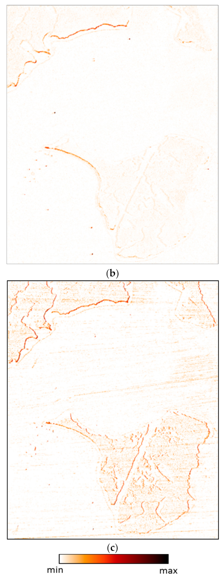
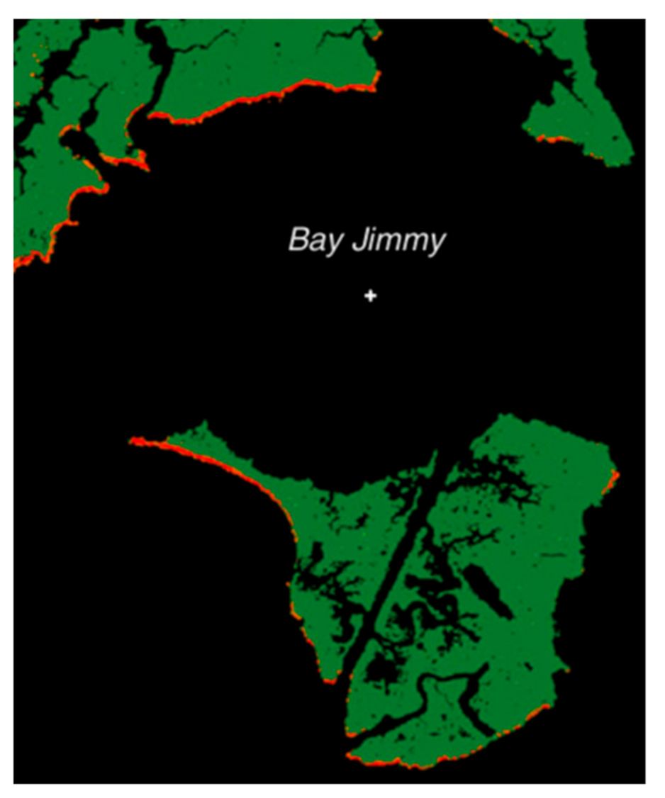
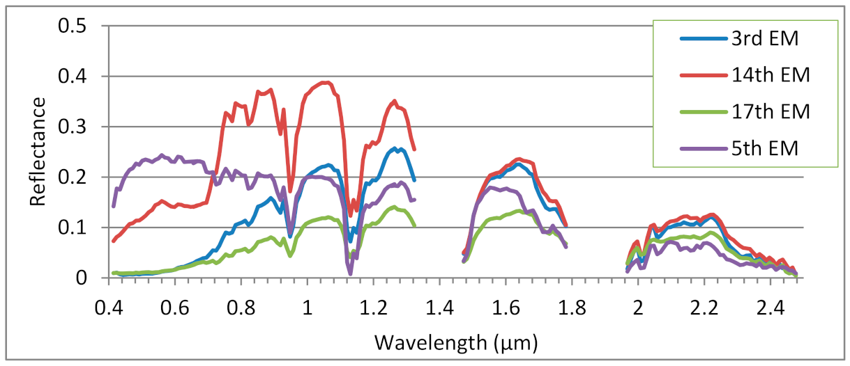
Spectral unmixing is used to extract the spectra of the pure materials present in the image, but as the image size or scene complexity increases, many endmembers can be extracted. In the cases of the synthetic image and DWH, spectral indices (Aera1700 and Area2300) were computed on the extracted endmembers to automatically select those of interest and map their abundance. Moreover, it was possible to distinguish the different types of HC+soil or sand mixtures in the simulated image, which is not possible using the existing spectral indices. In the case of DWH, even if the spectral index Area1700 has proven to be very efficient to map oiled coasts, combining spectral unmixing with Area1700 allowed a more detailed analysis of the polluted areas.

8. Conclusions

Several strategies have been developed to detect petroleum-contaminated soils. The first method uses spectral indices, specifically new ones that calculate the surfaces of the two main absorption bands of HC at 1.7 and 2.3 µm. The second is based on anomaly detection using prior knowledge to decrease the false-alarm rate. Finally, spectral unmixing was assessed using spectral indices to select endmembers of HC-bearing materials.

The cases studied cover a panel of different spill scenarios: intimate mixtures of soils and HC (“POC” case), oil deposited on the shoreline (“DWH” case), and a biodegraded tar pit on a former exploration site (“Tar pit” case). For each case, we demonstrated that the combination of two methods, anomaly detection and spectral indices to select anomalies of interest or spectral unmixing with spectral indices to select the endmembers of interest gave the most pertinent results.

HC indices have proven to be effective when HC spectral features are pronounced (cases POC and DWH), but there can be false positives due to dry vegetation for instance. Anomaly detection is also effective when there are few contaminated pixels in the image (POC and Tar pit cases) and can be an alternative method when the spectral characteristics of the HC are not sufficiently pronounced for the petroleum compounds to be efficiently detected (Tar Pit case). Furthermore, in most cases, the combination of anomaly detection and spectral index calculation reduced the number of false alarms as against using each method on its own. In the “POC” case for example, the logAUC was increased by approximately 50% for three of the four HC mixtures when the Area1700 spectral index was combined with the anomaly detection algorithm, compared to Area1700 on its own. Finally, spectral unmixing gave promising results (POC and DWH cases). More particularly, it enabled a finer analysis through the extraction of several distinct endmembers presenting HC spectral features, which is not possible with spectral indices.

The main advantages of all the proposed strategies are that they do not require spectral libraries containing oiled materials similar to those present in the images and are quasi-automatic. However, a disadvantage of all the methods using spectral indices is that they also detect plastic materials. This issue will be the subject of future work.

In this work, we focused on direct detection of petroleum-contaminated soil, but other recent studies (for instance [47,48,49]) have shown that vegetation health is a good indicator of soil pollution due to oil or gas. The combination of direct detection and vegetation health analysis opens up new perspectives for this work.