Meridional Changes in Satellite Chlorophyll and Fluorescence in Optically-Complex Coastal Waters of Northern Patagonia

Abstract

Northern Patagonia is one of the largest estuarine systems worldwide. It is characterized by complex geography, including islands, peninsulas, channels, and fjords. Here, the Inner Sea of Chiloé (ISC) is the largest estuarine system extending about 230 km in the meridional direction. Phytoplankton’s long-term dynamics and the main physical drivers of their variability are not well understood yet. Time-space fluctuations of Chlorophyll-a (Chl-a) and Chlorophyll fluorescence (nFLH) within the ISC and their association with meteorological and oceanographic processes were analyzed using high resolution (1000 m) satellite data (2003–2019). Our results revealed a meridional Chl-a and nFLH gradient along the ISC, with higher concentrations north of the Desertores islands where the topography promotes a semi-closed system with estuarine characteristics yearlong. Satellite Chl-a and nFLH were characterized by asynchronous seasonal cycles (nFLH peaks in fall) that differed from the southern ISC where the maximum Chl-a and nFLH occurs in spring-summer. The adjacent coastal ocean influences the southern ISC, and thus, the Chl-a and nFLH variability correlated well with the seasonal variation of meridional winds. The northern ISC was clearly influenced by river discharges, which can bias the Chl-a retrievals, decoupling the annual cycles of Chl-a and nFLH. In situ data from a buoy in Seno Reloncaví reaffirmed this bias in satellite Chl-a and a higher correlation with nFLH, by which the construction of a local Chl-a algorithm for northern Patagonia is essential.

1. Introduction

Coastal waters play a crucial role in the ecology and economy of coastal environments. It sustains fisheries (providing about 90% of global catches), aquaculture (which increases annually at a rate of 6%), and contributes with around 25% of global marine primary productivity, even though they cover a relatively small area [1]. Coastal waters are generally characterized by large variations in biological, physical and chemical properties and are an essential source of dissolved and particulate matter [2]. Coastal regions influenced by rivers and glaciers present additional complexities due to the significant freshwater inputs carrying constituents, such as suspended sediments, organic matter, and nutrients [3,4]. Thus, the study of coastal oceanographic processes based solely on field data typically lacks a high spatio-temporal coverage.

The synoptic coverage of satellite measurements allows us to quantify physical and biogeochemical parameters, providing valuable insights into coastal processes. The development of bio-optical algorithms provides valuable ocean color information associated with seawater constituents. They are commonly used in carbon cycling studies due to their ability to obtain estimates of phytoplankton biomass and primary productivity [2,5]. However, satellite chlorophyll observations are usually biased in coastal waters due to the high turbidity and complex optical properties.

Ocean primary production is modulated by processes at local, regional, and global scales [6] controlling the availability of nutrients and light [7]. In upwelling regions, such as the highly seasonal coastal ocean of northern Patagonia [8,9,10], the rise of nutrient-rich waters to the euphotic zone promotes high primary production [11]. River discharges also influence coastal productivity and biogeochemistry, modulating the supply of nutrients and organic matter from terrestrial/anthropogenic origin [12].

In northern Patagonia, the Inner Sea of Chiloé (ISC; 41${}^{\circ }$30${}^{\prime }$–44${}^{\circ }$00${}^{\prime }$S) provides multiple marine services, such as fish farming, shipping activity, mussel farming, fishing, and tourism. The ISC is a semi-closed system connected with the open ocean through Chacao channel and Boca del Guafo (Figure 1). Boca del Guafo is the largest water exchange area influencing the local circulation [13]. It presents elevated mixing in response to the influence of wind, tides, and the intrusions of Subantarctic Waters from the coastal ocean [14]. Seno Reloncaví, located on the northern edge of the ISC, is characterized by freshwater conditions (Figure 1). The high river discharges promote high turbidity and optically-complex conditions (Case II waters), similar to other estuarine systems [15,16]. In general, turbid conditions are characterized by increased suspended solids and dissolved organic matter, including CDOM (colored dissolved organic matter), affecting the performance of default Chlorophyll-a (Chl-a) ocean color algorithms [17,18]. A satellite chlorophyll algorithm has not been generated yet for the Inner Sea of Chiloé, mainly because of the lack of continuous In situ observations. However, a preliminary study has shown that default chlorophyll retrievals from Moderate Resolution Imaging Spectroradiometer (MODIS) do not perform well in the turbid conditions of northern Patagonia [19].

This study aims to assess the spatio-temporal distribution of remotely sensed chlorophyll (Chl-a) and fluorescence (Fluorescence Line Height, Chlorophyll fluorescence (nFLH)) and its relation with dominant oceanographic processes in the ISC for the period 2003–2019. Section 2 describes the data and methods. Section 3 highlights the main results associated with the importance of chlorophyll fluorescence in the northern ISC, where Chl-a seems to be highly biased. The discussion and main conclusions are presented in Section 4 and Section 5, respectively.

2. Data and Methods

2.1. Study Area

The Inner Sea of Chiloé, located in the southeastern Pacific ocean (Figure 1), has a latitudinal extension of c.a. 230 km and is the primary estuarine system of northern Patagonia [20,21]. Several islands (Desertores islands) generate an oceanographic barrier between the northern and southern basins. The northern ISC presents more estuarine characteristics because of several river discharges delivering freshwater and suspended materials, whereas the southern ISC has a significant marine influence due to the active water exchange through Boca del Guafo. The adjacent coastal ocean is mainly characterized by the presence of Subantarctic Waters (SAAW) and Equatorial Subsurface Waters (ESSW) [22]. The ISC receives significant freshwater from precipitation (between 2000 and 5000 mm per year) and river discharges [23,24].

2.2. Satellite Data

High resolution (1000 m) daily Chl-a and nFLH data from the Moderate Resolution Imaging Spectroradiometer (MODIS, on-board Aqua) were used for the period 2003–2019. The swath width of viewing is about 2330 km allowing MODIS to cover the entire Earth in 1–2 days. The spatial resolutions of MODIS bands are 250, 500, or 1000 m. Out of the 36 bands, 10 bands are useful for ocean color studies, with a spatial resolution of 1000 m [25]. The MODIS Aqua’s level-2 data were obtained from NASA’s (National Aeronautics and Space Administration) ocean color website (http://oceancolor.gsfc.nasa.gov, accessed on 1 September 2020). Standard procedures were used for Chl-a and nFLH estimates [26]. MODIS default algorithm is a fourth-degree polynomial algorithm that uses a maximum band ratio of 443, 448, and 551 nm wavelengths corresponding to spectral bands 9, 10, and 12, respectively [27]. The Ocean Biology Processing Group produces MODIS Chl-a and nFLH data (2014 reprocessing) at the Goddard Space Flight Center [28]. The quality controlled daily swaths were used to create gridded monthly composites at 1000 m horizontal resolution. The seasonal averages were computed considering Summer (January–March), Fall (April–June), Winter (July–September), and Spring (October–December). Considering that wind plays a crucial role in determining the spatial and temporal variability of phytoplankton blooms via surface advection and Ekman pumping in the coastal ocean [29], monthly wind fields were obtained from the Cross-Calibrated Multi-Platform (CCMP) project from Physical Oceanography Distributed Active Archive Center (PODAAC) website (https://podaac.jpl.nasa.gov/, accessed on 1 September 2020) for the period 2003–2019. The CCMP dataset combines cross-calibrated satellite winds obtained from Remote Sensing Systems (REMSS) using a Variational Analysis Method to produce high-resolution (0.25 degree) gridded fields [30]. To approximate the seasonal variability of surface circulation, AVISO (Archiving, Validation and Interpretation of Satellites Oceanographic Data) 2014 Delayed Time (DT14) gridded (0.25 degree) daily geostrophic velocities were obtained from the European Copernicus Marine Environment Monitoring Service (http://marine.copernicus.eu, accessed on 1 February 2021).

The meridional wind stress (MWS) was calculated following Montecinos and Balbontín [31]:

$${\tau }_y={\rho }_a\ast C_d\ast \left|v\right|\ast v,$$

(1)

where ${\tau }_y$ is the meridional component of the wind stress, ${\rho }_a$ is the air density (${\rho }_a$ = 1.22 kg ${\mathrm{m}}^3$), v is the meridional wind speed, and $C_d$ is the dimensionless drag coefficient ($C_d$ = 1.3 × ${10}^3$). Positive (negative) values of meridional wind stress indicate northward (southward) winds.

2.3. Field Data

In order to analyze the vertical structure of the water column under different environmental conditions, In situ data from two oceanographic cruises (August 2004 and July 2006) were analyzed (Figure 1). Both cruises sampled 13 stations along the ISC. At each station, hydrographic casts were carried out with a Seabird SBE-25 Conductivity-Temperature-Depth profiler mounted in a rosette equipped with 30 L Niskin bottles. From each Niskin bottle, filtered water was stored for dissolved nutrient analyses (phosphate, nitrate, and silicate) (see Reference [32]). Daily river discharge data were obtained from the Chilean General Water Department (Dirección General de Aguas). The gauging station (Carrera Basilio) is the closest to the Puelo River’s mouth and records a large fraction of the total freshwater outflow to northern Patagonia [33]. A comparison with a near-surface chlorophyll fluorescence time series from a buoy located in Seno Reloncaví (see Figure 1) was carried out to assess the performance of MODIS Chl-a and nFLH in northern ISC during 2017–2018. The data can be obtained at http://www.cdom.cl/estaciones.php?estacion=RLCV&seccion=Oceano (accessed on 1 October 2020).

2.4. Statistical Analyses

The main frequencies of spatio-temporal variability of Chl-a and nFLH were evaluated through a Multitaper Method-Singular Value Decomposition (MTM-SVD), following Correa-Ramírez and Hormazabal [34]. The MTM-SVD method detects statistically significant oscillations (frequency and period). The method also describes the frequencies of interest (i.e., annual cycle) through a time series reconstruction [35]. In using the MTM-SVD method, the local fractional variance spectra (LFV) were first calculated for Chl-a and nFLH. Then, the reconstructed time series and spatial fields were used to assess the link between Chl-a and nFLH and oceanographic processes in the ISC and coastal ocean. Once the frequency fields were reconstructed, the spatial structure was analyzed in terms of the explained variance (%) and phase (${}^{\circ }$) in significant frequency bands. While the first indicates the difference between the total variance and the variance of each significant frequency in a spatial context, the second shows the spread of this frequency along the spatial domain [36].

3. Results

3.1. Seasonal Variability of Wind and Geostrophic Flow

The seasonal variability of the wind field is shown in Figure 2a–d. A marked seasonality is observed off Chiloé Island with upwelling-favorable winds during summer (Figure 2b), and downwelling-favorable winds during fall-winter (Figure 2c,d). Furthermore, a meridional transition zone is found next to Boca del Guafo. Thus, upwelling-favorable winds are primarily located north of 44${}^{\circ }$S (Figure 2b) promoting the formation of a coastal upwelling thermal front [10]. The seasonal variability of the geostrophic flow field (Figure 2, lower panels) offers additional dynamical information on the surface circulation pattern. During spring-summer the formation of a pronounced northward jet is observed off Chiloé (Figure 2e,f), which is consistent with the formation of the coastal upwelling front [10]. During fall, a decrease in the magnitude of geostrophic velocities marks the transition to a predominantly southward flow in winter (Figure 2g,h) in response to changes in wind direction and sea level in the coastal band south of 35${}^{\circ }$S [37]. Notice that mean northward geostrophic currents appear within the ISC year-round suggesting an persistent connection between the Boca del Guafo and the ISC. Given the greater uncertainty of the satellite measurements in this relatively small basin, these data should be analyzed carefully. However, a northward geostrophic flow is consistent with the estuarine circulation reported by Sievers [38].

3.2. Seasonal Variability of Satellite Chl-a and nFLH

The seasonal climatology of Chl-a and nFLH fields shows an increased meridional gradient in the ISC. The maximum values of Chl-a and nFLH are confined to the northern sector (Figure 3). The highest mean Chl-a (>10 mg m${}^{-3}$) are uniformly distributed in the northern region in spring-summer (Figure 3a,b), whereas the higher values of Chl-a are restricted to the eastern margin in winter and fall (Figure 3c,d). The distribution of nFLH shows marked differences, compared to Chl-a, in the northern area (Figure 3e–h). This is especially evident in spring and summer, where the highest values of nFLH are primarily distributed around the western side of the basin (Figure 3e,f). The southern ISC showed a typical seasonal pattern for eastern boundary upwelling ecosystems, and revealed similar seasonality between Chl-a and nFLH with highest values in spring-summer. During fall, a marked decrease in Chl-a and nFLH is observed in the southern ISC (Figure 3c,g). This increases the meridional gradients, being largest for nFLH (Figure 3g).

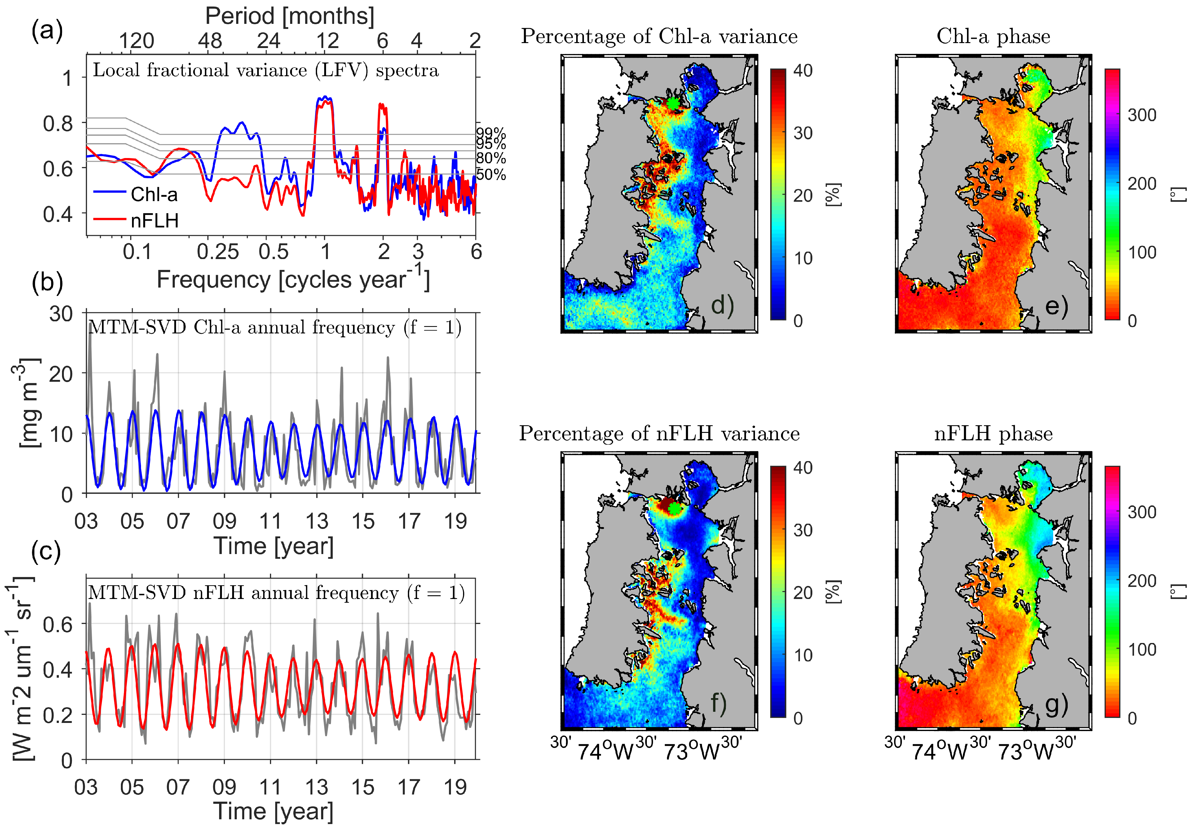
3.3. Spatio-Temporal Coupling/Decoupling between Chl-a and nFLH

The temporal variability of Chl-a and nFLH along the ISC is shown in Figure 4. The southern area (south of Desertores Islands; R3 and R4), where the ISC connects with the open ocean through Boca del Guafo (see Figure 1), presented a close co-variability with peaks during late spring and early summer (Figure 4b,c). The northern area, where the mean Chl-a is higher (Figure 3), presented a gradual decoupling between Chl-a and nFLH. Both variables presented joint variability. However, several Chl-a peaks are not consistent with maximum values of nFLH at R1 and R2. The peaks in nFLH (Chl-a) occur primarily in April–May (February–March) at R1 (Figure 4c). Thus, the coupling between Chl-a and nFLH increases in the southern direction along the ISC.

3.4. Spatio-Temporal Variability of Chl-a and nFLH along the ISC

During the 17 years of record, the dominant period of Chl-a variability was the annual oscillation (∼1 year; >99% confidence level), although a semiannual signal (∼180 days) was also significant (>95% confidence level). Other interannual frequencies (∼2 and 4 years) were also significant (>99%). The annual frequency of Chl-a and nFLH ranged between 10.8 and 13.2 months (Figure 5a). An interesting difference between Chl-a and nFLH was observed at low frequencies. Only Chl-a showed significant signals (>99%) in periods between 24 and 48 months (Figure 5a).

The spatial distribution of the variance explained by the annual Chl-a is represented in Figure 5d. In general, the variance explained was relatively high (>25%) around the northwestern area of the ISC and Boca del Guafo. A similar annual pattern is evidenced in nFLH (Figure 5f). In contrast, the Chl-a and nFLH annual variance was lower in the northeastern region of the ISC (<5%), where the semiannual frequency was dominant (>15%, not shown). The phase of the annual frequency was low along the entire western sector of the ISC (Figure 5e,g), confirming a synchronous annual variability between Chl-a and nFLH, with higher concentrations during summer (December–February), and lower values during winter (June–August) (Figure 5b,c). On the other hand, the phase varied to values around 120${}^{\circ }$ for Chl-a and 150${}^{\circ }$ for nFLH in northeastern ISC, revealing a decoupling of seasonality in this freshwater-influenced area (Figure 5e,g).

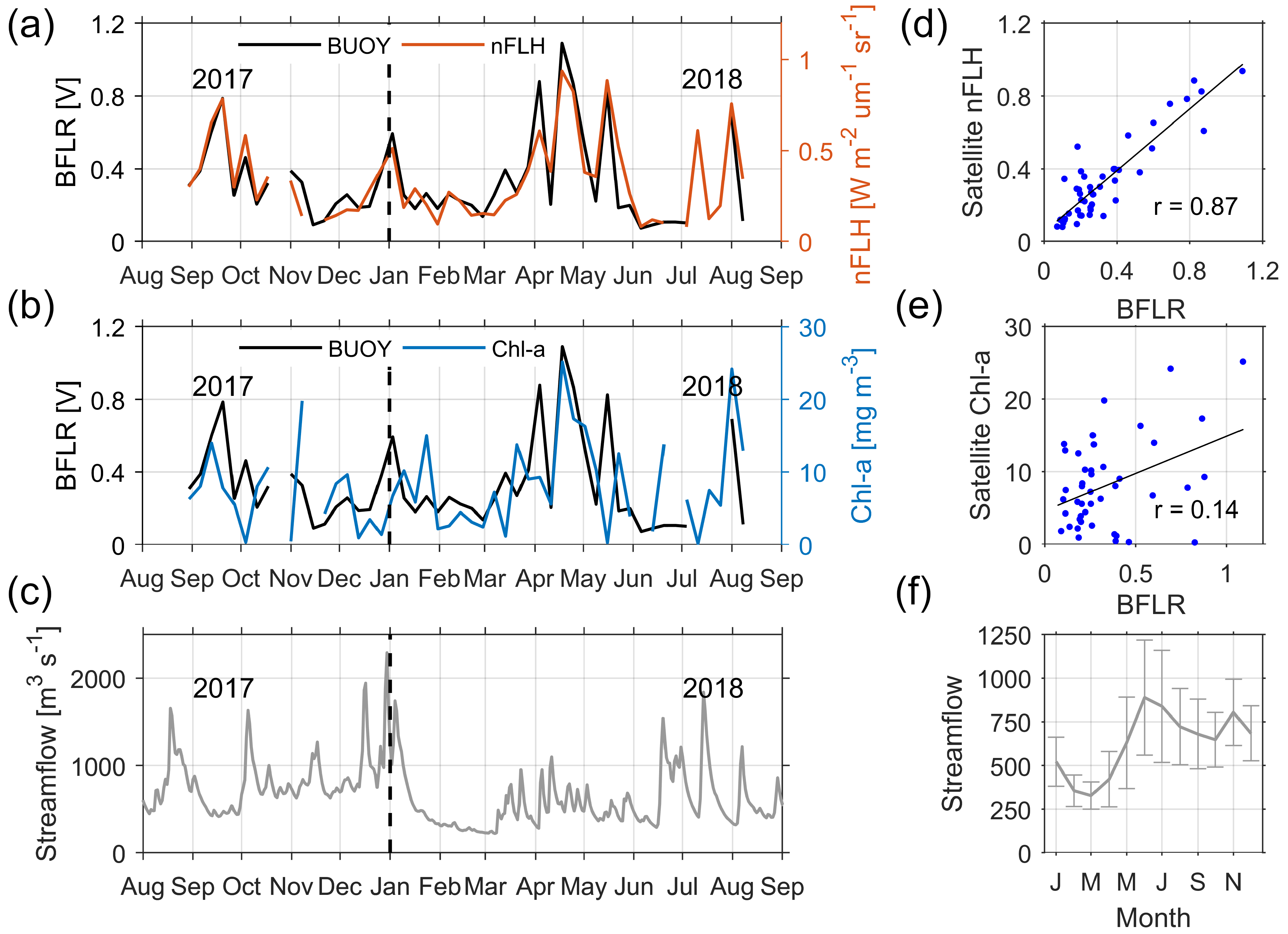
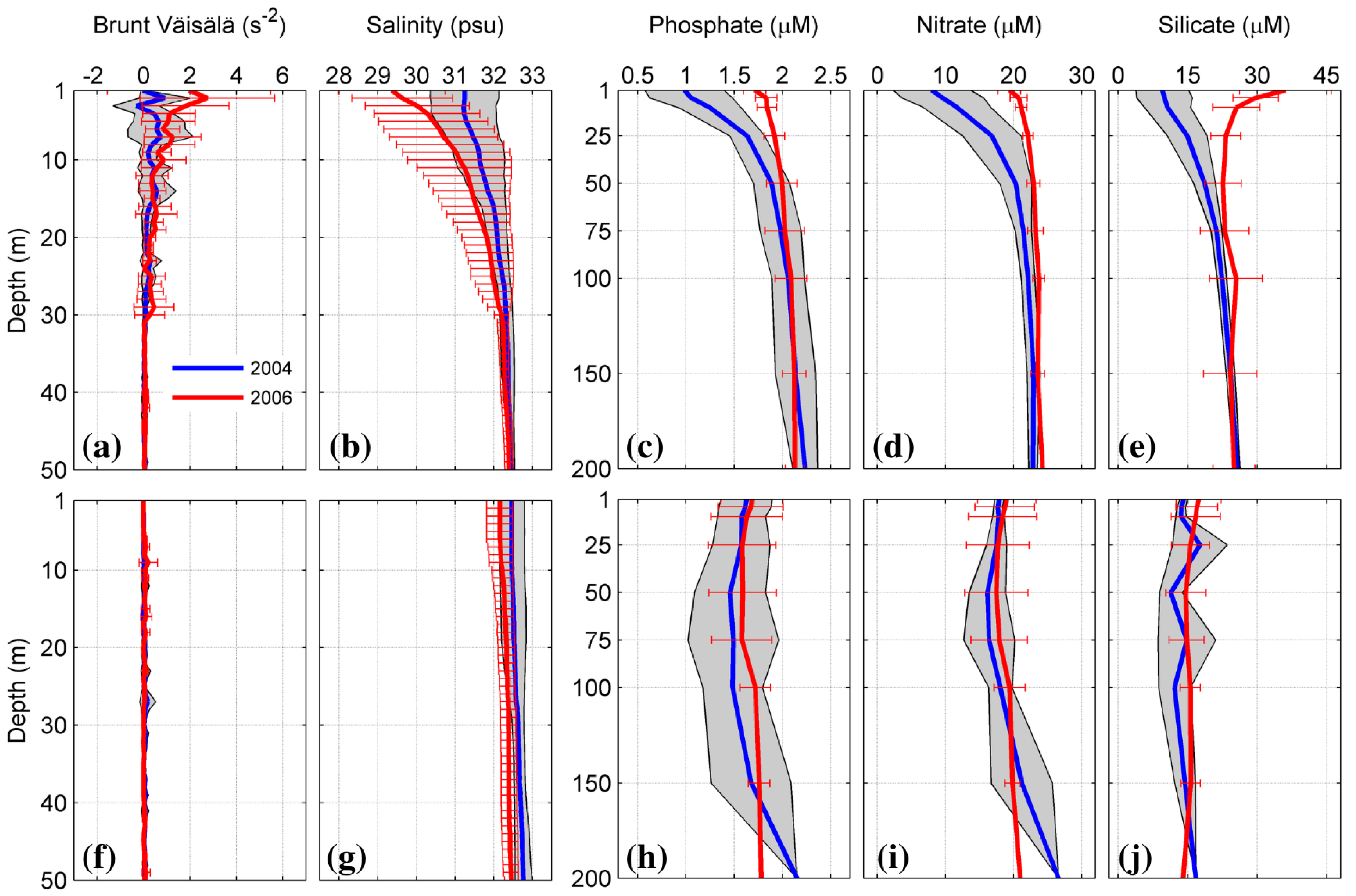
3.5. Oceanographic Processes Related to Chl-a and nFLH Variability

The meridional component of the wind stress was predominantly southward, with higher values during fall-winter, at Boca del Guafo. However, weaker and persistent northward winds were registered during spring-summer (Figure 6a). This would be linked to the development of coastal upwelling events off Chiloé Island in summer, potentially influencing the southern ISC via Boca del Guafo. Chl-a and nFLH varied synchronously in the southern ISC, which is confirmed by analyzing the time series in Boca del Guafo where peaks occurred in spring-summer (Figure 6b). The meridional wind stress showed positive correlations with both Chl-a and nFLH—high values of Chl-a and nFLH occurred under predominantly northward winds in spring-summer (Figure 6c). The latter may be associated with a greater supply of nutrients to the photic layer in response to the seasonal upwelling.

The spatial variability of the correlation between the meridional wind stress at Boca del Guafo and the Chl-a and nFLH along the ISC is shown in Figure 6f,g. Relatively high correlations (>0.5) were obtained along the western side of the ISC and its adjacent coastal ocean. A narrower and more coherent region of high correlations was found for nFLH (Figure 6e,g). The analysis highlighted the lack of temporal correlation with Chl-a and nFLH at the northeastern ISC (Figure 6f,g). Thus, it suggests that the Reloncaví basin responds to a different spatio-temporal dynamics.

The northeastern ISC is characterized by several river outflows with a pluvial-nival regime, which influences the stratification, the supply of nutrients, and the water’s optical properties. To analyze the evident decoupling between Chl-a and nFLH, time series were compared with In situ fluorescence observations from a buoy located at Seno Reloncaví (BFLR). Given the recent deployment of the oceanographic buoy (starting in 2017), this is the first time series comparison of satellite Chl-a and nFLH with In situ measurements. In situ measurements showed a seasonal signal with higher values during fall (Figure 7a,b). In general, the temporal variability of BFLR was well correlated (r = 0.87) with satellite nFLH (Figure 7a,d). Oppositely, the satellite Chl-a was poorly correlated (r = 0.14) with BFLR, particularly during spring-summer where several peaks observed by the satellite were inconsistent with the field data (Figure 7b). To further understand the differences between Chl-a and nFLH, and considering that river plumes are one of the most critical modulators of the optical properties of the ISC, Figure 7c shows the variability of Puelo River discharge. Its annual cycle presents two main peaks, during winter and spring, respectively (Figure 7f). Although the time series only covered a year, the highest coherence between Chl-a and nFLH were observed in fall when the river discharge was minimum (Figure 7a–c). In contrast, the largest mismatch between In situ fluorescence and satellite Chl-a occurred in winter and spring during peaks in freshwater discharges (Figure 7c). Thus, terrigenous materials must induce alterations in the optical properties, promoting errors in the quantification of Chl-a in northern ISC.

To evidence the influence of freshwater on satellite Chl-a retrievals, hydrographic and nutrient profiles were inspected for two years with contrasting river discharge regimes. Average profiles for all oceanographic stations north and south of Desertores Islands revealed a distinct vertical structure depending on the location and freshwater conditions. During the winter of 2006, the average river discharge was greater than 1600 m${}^3$ s${}^{-1}$, and a lower salinity and greater stratification characterized the northern ISC (Figure 8a,b). The river discharge only reached about 600 m${}^3$ s${}^{-1}$ during the winter of 2004, and consequently, weaker stratification and higher salinity values were observed (Figure 8a,b). In contrast, the southern ISC was characterized by more homogeneous profiles in both years with a lack of surface low-salinity layer (Figure 8f,g). Higher nutrient concentrations were observed in the northern ISC under higher river discharge conditions in 2006 (Figure 8c–e). Note that phosphate, nitrate, and particularly silicate showed a 25-m layer that was significantly higher during the high freshwater input period, which is most likely the result of the input of nutrient-rich river waters, in agreement with the vertical distribution of low-salinity water. Nutrient concentrations were similar in the surface layer of southern ISC, even under contrasting river discharge periods (Figure 8h–j).

4. Discussion

Satellite remote sensing is crucial for quantifying the spatio-temporal variability of physical and biogeochemical parameters in aquatic systems, particularly in regions with few field measurements [39]. Of particular interest is the remote sensing of phytoplankton pigments and dissolved and suspended matter. The wide range of composition of these substances poses a challenge in using satellite Chl-a retrievals in coastal waters [40]. Waters in which phytoplankton dominate the optical properties are classified as Case I waters. On the other hand, waters in which other constituents, such as suspended sediments and dissolved organic matter, dominate the optical properties are classified as Case II waters [41]. Coastal and estuarine waters, such as the ISC, often receive large freshwater discharges of fluvial and glacial origin with substantial loads of suspended organic and inorganic materials promoting an optically-complex environment—Case 2 waters [21,42].

Satellite Chl-a retrievals provide imprecise Chl-a estimates, hampering the understanding of the dynamics of primary productivity [17]. To better understand the spatio-temporal variability of phytoplankton biomass and its link with key oceanographic processes in the ISC, our study analyzed satellite Chl-a and nFLH for the period 2003–2019. The use of nFLH reduces the bias associated with Chl-a retrievals and is not affected by CDOM [43], standing as an improved indicator of physiological variability or phytoplankton biomass in some coastal regions [19].

The general meridional pattern of Chl-a and nFLH distribution (Figure 3 and Figure 4) were consistent with previous satellite-based results using coarser data for the ISC (e.g., Refs. [21,44]). The annual climatology (2003–2019) reveals distinct patterns related to geographical aspects of the entire basin. The northern ISC seems to be more productive throughout the year, splitting the ISC in two sub-basins separated by Desertores Islands (∼42${}^{\circ }$30${}^{\prime }$S) and regional circulation patterns [45]. Our results confirm the general patterns of Chl-a distribution [21,44] and provide new information regarding the spatio-temporal scales of variability of Chl-a and nFLH along the ISC. The southern ISC revealed a synchronous climatological pattern for Chl-a and nFLH with higher values observed during late spring and early summer, coupled with the seasonality of wind forcing [8,46,47]. However, the seasonal cycle of Chl-a and nFLH showed marked differences in the northern ISC and characterized by (i) a 2-month lag in the annual cycle of Chl-a compared to other regions of the ISC, and (ii) a 2-month lag between nFLH and Chl-a with higher values in fall. These large differences were associated with the influence of freshwater discharges from various rivers (e.g., Puelo River, Reñihue River) that provide allochthonous substances into the ISC [19,48]. Despite the meridional differences, the annual frequency of Chl-a and nFLH was spread between 10.8 and 13.2 months, resulting in a ±1.2-month displacement within the time series. This may be related to year-to-year changes in the phenology of phytoplankton biomass, similar to the coastal upwelling region off central-southern Chile [35,49].

Previous studies have revealed physical and biogeochemical variability in the ISC in response to interannual fluctuations of environmental forcing [21,47,50]. Overall, northern Patagonia’s atmospheric conditions present marked interannual variability [8,47]. The wind conditions around Boca del Guafo represented the regional variability. They revealed a climatological pattern with upwelling-favorable winds occurring in spring-summer, and fluctuations at interannual scale. These results are consistent with the findings of Garreaud [51] and Narváez et al. [8], suggesting that the seasonal and interannual variability of the regional wind is connected with large-scale climatic forcing (i.e., Pacific Decadal Oscillation, seasonal displacement of the South Pacific High, West Wind Drifts dynamics), and may also be related to intra-seasonal activity associated with the Madden-Julian Oscillation [52]. Our results confirm a synchronous annual cycle of Chl-a and nFLH in southern ISC and correlated with the meridional wind. This suggests an increase in the phytoplankton biomass in response to coastal upwelling events. Nonetheless, the entrance of nutrient-rich upwelling waters to the ISC through Boca del Guafo and its northward spreading is unclear. Furthermore, the high correlation between Chl-a and nFLH at Boca del Guafo suggests a lower influence of turbid freshwater plumes in summer and a fairly good performance of the Chl-a algorithm locally.

Boca del Guafo is the primary area for water exchange between the ISC and the open ocean with the presence of Subantarctic Waters and nutrient-rich Equatorial Subsurface Waters [22]. As noted by Narváez et al. [8], the influx of upwelling water into the ISC may cascade into nutrient availability changes and their relative concentrations, which could modulate the productivity and composition of phytoplankton. Furthermore, the variability of Chl-a and nFLH in the southwestern ISC was correlated with the adjacent coastal ocean suggesting a link with the mesoscale variability driven by coastal winds off southern Chile, which could explain the predominant annual cycles (Figure 5).

The northeastern area of the ISC was characterized by higher concentrations of Chl-a and nFLH throughout the year and contrasting annual cycles compared to those found in southern ISC (Figure 3 and Figure 4). The northern ISC is characterized by a shallower bathymetry and freshwater input from several rivers [13]. Our results confirmed that freshwater conditions promoted sharp vertical and horizontal salinity gradients (Figure 8), as proposed by previous studies [33,53,54,55]. These outflows generate an extended low-salinity tongue in the coastal ocean [24,56]. Moreover, the river runoff influences the nutrient composition of surface waters in northern Patagonia [50,57]. Our results were consistent with previous studies, showing a significant increase of silicate in the low-saline surface layer during a period of high river discharges (Figure 8). However, high phosphate and nitrate also characterized the surface freshwater layer, which could result from the mixing with oceanic waters.

Our results suggest a considerable bias of the Chl-a algorithm in northern ISC (Figure 7). The supply of terrigenous materials from large rivers and ice melt (e.g., CDOM and particulate materials) would modify the optical properties of seawater [58] through the formation of turbidity plumes, challenging the study of phytoplankton dynamics. Our results revealed marked differences in the temporal patterns of Chl-a and nFLH in northern ISC, including a lag in the annual cycle and inconsistencies in the intra-seasonal peaks (Figure 4). In situ fluorescence data from the buoy located in Seno Reloncaví showed a high correlation with the nFLH and coherent peaks during fall (Figure 7). The better performance of nFLH in this region supports previous results evaluating it with shipboard chlorophyll estimates [19]. Our results indicate that the largest differences between the In situ data and satellite Chl-a were recorded during events of high river discharge. The satellite Chl-a data seems to work better in fall, the period with the lowest river discharge and peaks in phytoplankton biomass [55].

At low frequencies, the local fractional variance (LFV) spectra showed differences between Chl-a and nFLH. During the 17-year time series, interannual frequencies (∼3–4 years) were highly significant (>99% confidence level) for Chl-a. However, these frequencies were not observed for nFLH (Figure 5). This interannual variability in Chl-a could be attributed to low-frequency processes incorporating colored materials and sediments into the ISC (e.g., river discharges, glacier melting, etc.) instead phytoplankton biomass variability. This is of particular interest considering that remote and large-scale climatic-oceanographic phenomena can alter the precipitation [59] and ocean temperatures [21] on interannual scales, as well as the modulation of freshwater discharges from rivers in central-southern Chile and northern Patagonia [60,61]. This study highlights the use of nFLH [19,43,62] to avoid the interference from other components in assessing the chlorophyll variability in the optically-complex waters of the ISC. Future studies should focus on the generation of a local Chl-a algorithm incorporating the meridional optical gradients of Chl-a and nFLH to further understand biophysical processes modulating the variability of phytoplankton biomass in the ISC.

5. Summary

The coastal ocean of northern Patagonia is a highly productive ecosystem with socio-economic implications. The study of coastal productivity and its variability has been barely analyzed historically because of a lacking continuous monitoring. The study area, including the Inner Sea of Chiloé (ISC), is characterized by high spatial variability in oceanographic and optically-complex conditions. Consequently, the use of default satellite Chl-a algorithms to monitor its coastal productivity is challenging. This study analyzes the spatio-temporal variability of both Chl-a and nFLH along the meridional gradient of the ISC and its adjacent coastal ocean. Our results highlight four main findings; (i) there is a decoupling between the Chl-a and nFLH in the northern ISC (north of Desertores Islands), (ii) the annual cycles of Chl-a and nFLH are synchronous in the southern ISC with peaks in spring-summer, (iii) the wind forcing correlated well with the variability of Chl-a and nFLH in the southern ISC, with maximum values associated with northward winds, and (iv) the nFLH agrees well with In situ measurements in Seno Reloncaví, whereas the satellite Chl-a was poorly correlated in In situ data during periods of high river discharge. The high contrast in oceanographic conditions between the northern and southern ISC suggests that the elevated loads of suspended and dissolved materials associated with turbid river plumes influences negatively the satellite readings of Chl-a in the Case II waters of northern ISC. Future studies evaluating the implementation of a new local Chl-a algorithm are crucial for northern Patagonia to properly quantify coastal productivity changes at different spatio-temporal scales.

References

1. Colella, S.; Falcini, F.; Rinaldi, E.; Sammartino, M.; Santoleri, R. Mediterranean ocean colour chlorophyll trends. PLoS ONE 2016, 11, e0155756. [Google Scholar] [CrossRef] [Green Version]
2. D’sa, E.J.; Miller, R.L.; Del Castillo, C. Bio-optical properties and ocean color algorithms for coastal waters influenced by the Mississippi River during a cold front. Appl. Opt. 2006, 45, 7410–7428. [Google Scholar] [CrossRef] [PubMed]
3. Saldías, G.S.; Kipp Shearman, R.; Barth, J.A.; Tufillaro, N. Optics of the offshore Columbia River plume from glider observations and satellite imagery. J. Geophys. Res. Ocean. 2016, 121, 2367–2384. [Google Scholar] [CrossRef] [Green Version]
4. Vargas, C.A.; Cuevas, L.A.; Silva, N.; González, H.E.; De Pol-Holz, R.; Narváez, D.A. Influence of glacier melting and river discharges on the nutrient distribution and DIC recycling in the southern Chilean Patagonia. J. Geophys. Res. Biogeosci. 2018, 123, 256–270. [Google Scholar] [CrossRef]
5. Hao, Q.; Chai, F.; Xiu, P.; Bai, Y.; Chen, J.; Liu, C.; Le, F.; Zhou, F. Spatial and temporal variation in chlorophyll a concentration in the Eastern China Seas based on a locally modified satellite dataset. Estuar. Coast. Shelf Sci. 2019, 220, 220–231. [Google Scholar] [CrossRef]
6. Falkowski, P.G.; Barber, R.T.; Smetacek, V. Biogeochemical controls and feedbacks on ocean primary production. Science 1998, 281, 200–206. [Google Scholar] [CrossRef] [Green Version]
7. Picado, A.; Alvarez, I.; Vaz, N.; Dias, J.M. Chlorophyll concentration along the northwestern coast of the Iberian Peninsula vs. atmosphere-ocean-land conditions. J. Coast. Res. 2013, 65, 2047–2052. [Google Scholar] [CrossRef]
8. Narváez, D.A.; Vargas, C.A.; Cuevas, L.A.; García-Loyola, S.A.; Lara, C.; Segura, C.; Tapia, F.J.; Broitman, B.R. Dominant scales of subtidal variability in coastal hydrography of the Northern Chilean Patagonia. J. Mar. Syst. 2019, 193, 59–73. [Google Scholar] [CrossRef]
9. Pérez-Santos, I.; Seguel, R.; Schneider, W.; Linford, P.; Donoso, D.; Navarro, E.; Amaya-Cárcamo, C.; Pinilla, E.; Daneri, G. Synoptic-scale variability of surface winds and ocean response to atmospheric forcing in the eastern austral Pacific Ocean. Ocean Sci. 2019, 15, 1247–1266. [Google Scholar] [CrossRef] [Green Version]
10. Saldías, G.S.; Hernández, W.; Lara, C.; Muñoz, R.; Rojas, C.; Vásquez, S.; Pérez-Santos, I.; Soto-Mardones, L. Seasonal Variability of SST Fronts in the Inner Sea of Chiloé and Its Adjacent Coastal Ocean, Northern Patagonia. Remote Sens. 2021, 13, 181. [Google Scholar] [CrossRef]
11. Rykaczewski, R.R.; Checkley, D.M. Influence of ocean winds on the pelagic ecosystem in upwelling regions. Proc. Natl. Acad. Sci. USA 2008, 105, 1965–1970. [Google Scholar] [CrossRef] [PubMed] [Green Version]
12. Vörösmarty, C.; Fekete, B.M.; Meybeck, M.; Lammers, R.B. Global system of rivers: Its role in organizing continental land mass and defining land-to-ocean linkages. Glob. Biogeochem. Cycles 2000, 14, 599–621. [Google Scholar] [CrossRef] [Green Version]
13. Iriarte, J.L.; González, H.E.; Nahuelhual, L. Patagonian fjord ecosystems in southern Chile as a highly vulnerable region: Problems and needs. Ambio 2010, 39, 463–466. [Google Scholar] [CrossRef] [PubMed] [Green Version]
14. Ramírez, B.; Pizarro, E. Distribución de clorofila ay feopigmentos en los canales australes chilenos comprendidos entre Puerto Montt y la laguna San Rafael, Chile. Cienc. Tecnol. Mar. 2005, 28, 45–62. [Google Scholar]
15. Chen, Z.; Muller-Karger, F.E.; Hu, C. Remote sensing of water clarity in Tampa Bay. Remote Sens. Environ. 2007, 109, 249–259. [Google Scholar] [CrossRef]
16. Gitelson, A.A.; Schalles, J.F.; Hladik, C.M. Remote chlorophyll-a retrieval in turbid, productive estuaries: Chesapeake Bay case study. Remote Sens. Environ. 2007, 109, 464–472. [Google Scholar] [CrossRef]
17. Dall’Olmo, G.; Gitelson, A.A.; Rundquist, D.C.; Leavitt, B.; Barrow, T.; Holz, J.C. Assessing the potential of SeaWiFS and MODIS for estimating chlorophyll concentration in turbid productive waters using red and near-infrared bands. Remote Sens. Environ. 2005, 96, 176–187. [Google Scholar] [CrossRef]
18. Schalles, J.F. Optical remote sensing techniques to estimate phytoplankton chlorophyll a concentrations in coastal waters with varying suspended matter and CDOM concentrations. In Remote Sensing of Aquatic Coastal Ecosystem Processes; Springer: Dordrecht, The Netherlands, 2006; pp. 27–79. [Google Scholar]
19. Lara, C.; Saldías, G.S.; Westberry, T.K.; Behrenfeld, M.J.; Broitman, B.R. First assessment of MODIS satellite ocean color products (OC3 and nFLH) in the Inner Sea of Chiloé, northern Patagonia. Lat. Am. J. Aquat. Res. 2017, 45, 822–827. [Google Scholar] [CrossRef]
20. Palma, S.; Silva, N. Distribution of siphonophores, chaetognaths, euphausiids and oceanographic conditions in the fjords and channels of southern Chile. Deep Sea Res. Part II Top. Stud. Oceanogr. 2004, 51, 513–535. [Google Scholar] [CrossRef]
21. Lara, C.; Saldías, G.S.; Tapia, F.J.; Iriarte, J.L.; Broitman, B.R. Interannual variability in temporal patterns of Chlorophyll–a and their potential influence on the supply of mussel larvae to inner waters in northern Patagonia (41–44 S). J. Mar. Syst. 2016, 155, 11–18. [Google Scholar] [CrossRef]
22. Silva, N.; Calvete, C.; Sievers, H. Características oceanográficas físicas y químicas de canales australes chilenos entre Puerto Montt y Laguna San Rafael (Crucero Cimar-Fiordo 1). Cienc. Tecnol. Mar. 1997, 20, 23–106. [Google Scholar]
23. Lara, A.; Villalba, R.; Urrutia, R. A 400-year tree-ring record of the Puelo River summer–fall streamflow in the Valdivian Rainforest eco-region, Chile. Clim. Chang. 2008, 86, 331–356. [Google Scholar] [CrossRef]
24. Saldías, G.S.; Sobarzo, M.; Quiñones, R. Freshwater structure and its seasonal variability off western Patagonia. Prog. Oceanogr. 2019, 174, 143–153. [Google Scholar] [CrossRef]
25. Abbas, M.M.; Melesse, A.M.; Scinto, L.J.; Rehage, J.S. Satellite Estimation of Chlorophyll-a Using Moderate Resolution Imaging Spectroradiometer (MODIS) Sensor in Shallow Coastal Water Bodies: Validation and Improvement. Water 2019, 11, 1621. [Google Scholar] [CrossRef] [Green Version]
26. O’Reilly, J.E.; Maritorena, S.; Siegel, D.A.; O’Brien, M.C.; Toole, D.; Mitchell, B.G.; Kahru, M.; Chavez, F.P.; Strutton, P.; Cota, G.F.; et al. Ocean color chlorophyll a algorithms for SeaWiFS, OC2, and OC4: Version 4. SeaWiFS Postlaunch Calibration Valid. Anal. Part 2000, 3, 9–23. [Google Scholar]
27. Hu, C.; Lee, Z.; Franz, B. Chlorophyll aalgorithms for oligotrophic oceans: A novel approach based on three-band reflectance difference. J. Geophys. Res. Ocean. 2012, 117. [Google Scholar] [CrossRef] [Green Version]
28. Feldman, G.; McClain, C. Ocean Color Web—SeaWiFS Reprocessing 2010.0, MODIS-Terra Reprocessing 2013.0, MODIS-Aqua Reprocessing 2013.1, VIIRS-SNPP Reprocessing 2014.0. NASA Goddard Space Flight Center, 2014. Available online: http://oceancolor.gsfc.nasa.gov/ (accessed on 1 September 2020).
29. Raitsos, D.E.; Pradhan, Y.; Brewin, R.J.; Stenchikov, G.; Hoteit, I. Remote sensing the phytoplankton seasonal succession of the Red Sea. PLoS ONE 2013, 8, e64909. [Google Scholar] [CrossRef] [Green Version]
30. Atlas, R.; Hoffman, R.; Ardizzone, J.; Leidner, S.; Jusem, J. Development of a new cross-calibrated, multi-platform (CCMP) ocean surface wind product. In Proceedings of the AMS 13th Conference on Integrated Observing and Assimilation Systems for Atmosphere, Oceans, and Land Surface (IOAS-AOLS), Phoenix, AZ, USA, 10 January 2009. [Google Scholar]
31. Montecinos, A.; Balbontín, F. Indices de surgencia y circulación superficial del mar: Implicancias biológicas en un área de desove de peces entre Los Vilos y Valparaíso, Chile. Rev. Biol. Mar 1993, 28, 133–150. [Google Scholar]
32. Silva, N.; Guerra, D. Distribución de temperatura, salinidad, oxígeno disuelto y nutrientes en el canal Pulluche-Chacabuco, Chile.(Crucero CIMAR 9 fiordos). Cienc. Tecnol. Mar 2008, 31, 29–43. [Google Scholar]
33. Valle-Levinson, A.; Sarkar, N.; Sanay, R.; Soto, D.; León, J. Spatial structure of hydrography and flow in a Chilean fjord, Estuario Reloncavi. Estuaries Coasts 2007, 30, 113–126. [Google Scholar] [CrossRef]
34. Correa-Ramirez, M.; Hormazabal, S. MultiTaper method-singular value decomposition (MTM-SVD): Spatial-frequency variability of the sea level in the southeastern Pacific. Lat. Am. J. Aquat. Res. 2012, 40, 1039–1060. [Google Scholar] [CrossRef]
35. Morales, C.E.; Hormazabal, S.; Andrade, I.; Correa-Ramirez, M.A. Time-space variability of chlorophyll-a and associated physical variables within the region off Central-Southern Chile. Remote Sens. 2013, 5, 5550–5571. [Google Scholar] [CrossRef] [Green Version]
36. Wallace, J.M.; Gutzler, D.S. Teleconnections in the geopotential height field during the Northern Hemisphere winter. Mon. Weather Rev. 1981, 109, 784–812. [Google Scholar] [CrossRef]
37. Strub, P.T.; James, C.; Montecino, V.; Rutllant, J.A.; Blanco, J.L. Ocean circulation along the southern Chile transition region (38–46 S): Mean, seasonal and interannual variability, with a focus on 2014–2016. Prog. Oceanogr. 2019, 172, 159–198. [Google Scholar] [CrossRef] [PubMed]
38. Sievers, H. Water masses and circulation in austral Chilean channels and fjords. In Progress in the Oceanographic Knowledge of Chilean Interior Waters, from Puerto Montt to Cape Horn; Comité Oceanográfico Nacional—Pontificia Universidad Católica de Valparaíso: Valparaíso, Chile, 2008; pp. 53–58. [Google Scholar]
39. Spyrakos, E.; O’Donnell, R.; Hunter, P.D.; Miller, C.; Scott, M.; Simis, S.G.; Neil, C.; Barbosa, C.C.; Binding, C.E.; Bradt, S.; et al. Optical types of inland and coastal waters. Limnol. Oceanogr. 2018, 63, 846–870. [Google Scholar] [CrossRef] [Green Version]
40. Mélin, F.; Vantrepotte, V. How optically diverse is the coastal ocean? Remote Sens. Environ. 2015, 160, 235–251. [Google Scholar] [CrossRef]
41. Morel, A.; Prieur, L. Analysis of variations in ocean color 1. Limnol. Oceanogr. 1977, 22, 709–722. [Google Scholar] [CrossRef]
42. Sarthyendranath, S. Remote Sensing of Ocean Colour in Coastal, and Other Optically-Complex Waters. In Reports of the International Ocean-Colour; Sathyendranath, S., Ed.; International Ocean Colour Coordinating Group (IOCCG): Dartmouth, NS, Canada, 2000. [Google Scholar]
43. Behrenfeld, M.J.; Westberry, T.K.; Boss, E.S.; O’Malley, R.T.; Siegel, D.A.; Wiggert, J.D.; Franz, B.; McLain, C.; Feldman, G.; Doney, S.C.; et al. Satellite-detected fluorescence reveals global physiology of ocean phytoplankton. Biogeosciences 2009, 6, 779. [Google Scholar] [CrossRef] [Green Version]
44. Rodriguez-Benito, C.; Alfredo Tello, G. Characterization of mesoscale spatio-temporal patterns and variability of remotely sensed Chl a and SST in the Interior Sea of Chiloe (41.4–43.5° S). Int. J. Remote Sens. 2009, 30, 1521–1536. [Google Scholar]
45. Silva, N.; Vargas, C.A. Hypoxia in Chilean patagonian fjords. Prog. Oceanogr. 2014, 129, 62–74. [Google Scholar] [CrossRef]
46. Montero, P.; Daneri, G.; Gonzalez, H.E.; Iriarte, J.L.; Tapia, F.J.; Lizarraga, L.; Sanchez, N.; Pizarro, O. Seasonal variability of primary production in a fjord ecosystem of the Chilean Patagonia: Implications for the transfer of carbon within pelagic food webs. Cont. Shelf Res. 2011, 31, 202–215. [Google Scholar] [CrossRef]
47. Garreaud, R.; Lopez, P.; Minvielle, M.; Rojas, M. Large-scale control on the Patagonian climate. J. Clim. 2013, 26, 215–230. [Google Scholar] [CrossRef]
48. Silva, N.; Vargas, C.A.; Prego, R. Land–ocean distribution of allochthonous organic matter in surface sediments of the Chiloé and Aysén interior seas (Chilean Northern Patagonia). Cont. Shelf Res. 2011, 31, 330–339. [Google Scholar] [CrossRef]
49. Corredor-Acosta, A.; Morales, C.E.; Hormazabal, S.; Andrade, I.; Correa-Ramirez, M.A. Phytoplankton phenology in the coastal upwelling region off central-southern C hile (35° S–38° S): Time-space variability, coupling to environmental factors, and sources of uncertainty in the estimates. J. Geophys. Res. Ocean. 2015, 120, 813–831. [Google Scholar] [CrossRef]
50. Iriarte, J.L.; Pantoja, S.; Daneri, G. Oceanographic processes in Chilean fjords of Patagonia: From small to large-scale studies. PrOce 2014, 129, 1–7. [Google Scholar] [CrossRef]
51. Garreaud, R. Record-breaking climate anomalies lead to severe drought and environmental disruption in western Patagonia in 2016. Clim. Res. 2018, 74, 217–229. [Google Scholar] [CrossRef]
52. Jacques-Coper, M.; Brönnimann, S.; Martius, O.; Vera, C.S.; Cerne, S.B. Evidence for a modulation of the intraseasonal summer temperature in Eastern Patagonia by the Madden-Julian Oscillation. J. Geophys. Res. Atmos. 2015, 120, 7340–7357. [Google Scholar] [CrossRef] [Green Version]
53. Calvete, C.; Sobarzo, M. Quantification of the surface brackish water layer and frontal zones in southern Chilean fjords between Boca del Guafo (43°30S) and Estero Elefantes (46°30S). Cont. Shelf Res. 2011, 31, 162–171. [Google Scholar] [CrossRef]
54. Pérez-Santos, I.; Garcés-Vargas, J.; Schneider, W.; Ross, L.; Parra, S.; Valle-Levinson, A. Double-diffusive layering and mixing in Patagonian fjords. Prog. Oceanogr. 2014, 129, 35–49. [Google Scholar] [CrossRef]
55. Iriarte, J.; León-Muñoz, J.; Marcé, R.; Clément, A.; Lara, C. Influence of seasonal freshwater streamflow regimes on phytoplankton blooms in a Patagonian fjord. N. Z. J. Mar. Freshw. Res. 2017, 51, 304–315. [Google Scholar] [CrossRef]
56. Dávila, P.M.; Figueroa, D.; Müller, E. Freshwater input into the coastal ocean and its relation with the salinity distribution off austral Chile (35–55 S). Cont. Shelf Res. 2002, 22, 521–534. [Google Scholar] [CrossRef]
57. Aracena, C.; Lange, C.B.; Iriarte, J.L.; Rebolledo, L.; Pantoja, S. Latitudinal patterns of export production recorded in surface sediments of the Chilean Patagonian fjords (41–55 S) as a response to water column productivity. Cont. Shelf Res. 2011, 31, 340–355. [Google Scholar] [CrossRef]
58. Jacob, B.G.; Tapia, F.J.; Daneri, G.; Iriarte, J.L.; Montero, P.; Sobarzo, M.; Quiñones, R.A. Springtime size-fractionated primary production across hydrographic and PAR-light gradients in Chilean Patagonia (41–50 S). Prog. Oceanogr. 2014, 129, 75–84. [Google Scholar] [CrossRef]
59. Daniels, L.D.; Veblen, T.T. ENSO effects on temperature and precipitation of the Patagonian-Andean region: Implications for biogeography. Phys. Geogr. 2000, 21, 223–243. [Google Scholar] [CrossRef]
60. Saldías, G.S.; Largier, J.L.; Mendes, R.; Pérez-Santos, I.; Vargas, C.A.; Sobarzo, M. Satellite-measured interannual variability of turbid river plumes off central-southern Chile: Spatial patterns and the influence of climate variability. Prog. Oceanogr. 2016, 146, 212–222. [Google Scholar] [CrossRef]
61. Sepúlveda, J.; Pantoja, S.; Hughen, K.A.; Bertrand, S.; Figueroa, D.; León, T.; Drenzek, N.J.; Lange, C. Late Holocene sea-surface temperature and precipitation variability in northern Patagonia, Chile (Jacaf Fjord, 44 S). Quat. Res. 2009, 72, 400–409. [Google Scholar] [CrossRef]
62. Hu, C.; Muller-Karger, F.E.; Taylor, C.J.; Carder, K.L.; Kelble, C.; Johns, E.; Heil, C.A. Red tide detection and tracing using MODIS fluorescence data: A regional example in SW Florida coastal waters. Remote Sens. Environ. 2005, 97, 311–321. [Google Scholar] [CrossRef]
Figure 1. (a) Map of northern Patagonia. The Inner Sea of Chiloé (ISC) is enclosed in a red box and shown in (b,c). Black circles correspond to the location of oceanographic profiles shown in Figure 8. PR corresponds to the location of the Puelo River. The blue circle corresponds to the location of the oceanographic buoy in Seno Reloncavi. The average values of Moderate Resolution Imaging Spectroradiometer (MODIS) Chlorophyll-a (Chl-a) and Chlorophyll fluorescence (nFLH) (2003–2019) are color-coded in (ac), respectively.
Remotesensing 13 01026 g001
Figure 2. Seasonal climatologies of (upper panels) CCMP satellite wind vectors and (lower panels) AVISO satellite geostrophic velocities (2003–2019) for (a,e) spring (October, November, December), (b,f) summer (January, February, March), (c,g) fall (April, May, June), and (d,h) winter (July, August, September). The colors in (ad) represent the wind speed. For reference of locations, see Figure 1a.
Remotesensing 13 01026 g002
Figure 3. Seasonal climatologies of (upper panels) Chl-a and (lower panels) nFLH computed from all daily MODIS-Aqua images (2003–2019) for (a,e) spring (October, November, December), (b,f) summer (January, February, March), (c,g) fall (April, May, Jun), and (d,h) winter (July, August, September). For reference of locations, see Figure 1a.
Remotesensing 13 01026 g003
Figure 4. Temporal variability of Chl-a (blue curves) and nFLH (red curves) at 4 locations (R1–R4, shown as blue boxes in (a) along the Inner Sea of Chiloé (ISC). The interannual time series are presented in (b), whereas the corresponding annual cycles are shown in (c); r-values correspond to linear correlation coefficients. The average Chl-a is color-coded in (a). Notice that the annual cycles start from June in (c). For reference of locations, see Figure 1a.
Remotesensing 13 01026 g004
Figure 5. (a) Local fractional variance (LFV) spectra for Chl-a (blue curves) and nFLH (red curves). The values on the right hand side y-axis shows the confidence levels (%). Original time series (black lines) and reconstructed annual cycle (blue and red lines) for Chl-a and nFLH are shown in (b,c), respectively, for the location specified with a green asterisk in (d,f). The spatial field of explained annual variance and the corresponding phase is presented for Chl-a (d,e) and nFLH (f,g). For reference of locations, see Figure 1a.
Remotesensing 13 01026 g005
Figure 6. Time series of mean (a) meridional wind stress and (b) Chl-a and nFLH at Boca del Guafo (region between 73 –74 W and 43 –44 S). (c) Chl-a and nFLH concentration as function of meridional wind stress. Spatial fields of linear correlation coefficient between meridional wind stress at Boca del Guafo and Chl-a (df) and nFLH (eg). The Inner Sea of Chiloé (ISC) is enclosed in a blue box and shown in (f,g) for better visualization. For reference of locations, see Figure 1a.
Remotesensing 13 01026 g006
Figure 7. Comparison between near-surface (1 m) In situ fluorescence (7-day averages) and (a,d) nFLH and (b,e) Chl-a. r-values correspond to linear correlation coefficients. Puelo river discharge and its annual cycle is presented in (c,f), respectively. For reference of the buoy location, see Figure 1a.
Remotesensing 13 01026 g007
Figure 8. Mean vertical profiles of: (a,f) Brunt-Väisälä frequency, (b,g) Salinity, (c,h) phosphate, (d,i) nitrate, and (e,j) silicate. Top (bottom) panels correspond to profiles north (south) of Desertores Islands (see Figure 1) for the winter of 2004 (blue) and the winter of 2006 (red). For reference of the location of the oceanographic stations, see Figure 1b,c.
Remotesensing 13 01026 g008
Publisher’s Note: MDPI stays neutral with regard to jurisdictional claims in published maps and institutional affiliations.