
Assimilation of LAI Derived from UAV Multispectral Data into the SAFY Model to Estimate Maize Yield

1
College of Mechanical and Electronic Engineering, Northwest A&F University, Yangling 712100, China
2
Key Laboratory of Agricultural Internet of Things, Ministry of Agriculture, Yangling 712100, China
3
Institute of Soil and Water Conservation, Northwest A&F University, Yangling 712100, China
4
College of Information, Xi’an University of Finance and Economics, Xi’an 710100, China
*
Author to whom correspondence should be addressed.
Remote Sens. 2021, 13(6), 1094; https://0-doi-org.brum.beds.ac.uk/10.3390/rs13061094
Submission received: 8 February 2021
/
Revised: 7 March 2021
/
Accepted: 10 March 2021
/
Published: 13 March 2021
(This article belongs to the Special Issue Earth Observations and Crop Models for Sustainable Agricultural Management: Part II)
Abstract
:In this study, we develop a method to estimate corn yield based on remote sensing data and ground monitoring data under different water treatments. Spatially explicit information on crop yields is essential for farmers and agricultural agencies to make well-informed decisions. One approach to estimate crop yield with remote sensing is data assimilation, which integrates sequential observations of canopy development from remote sensing into model simulations of crop growth processes. We found that leaf area index (LAI) inversion based on unmanned aerial vehicle (UAV) vegetation index has a high accuracy, with R2 and root mean square error (RMSE) values of 0.877 and 0.609, respectively. Maize yield estimation based on UAV remote sensing data and simple algorithm for yield (SAFY) crop model data assimilation has different yield estimation accuracy under different water treatments. This method can be used to estimate corn yield, where R2 is 0.855 and RMSE is 692.8kg/ha. Generally, the higher the water stress, the lower the estimation accuracy. Furthermore, we perform the yield estimate mapping at 2 m spatial resolution, which has a higher spatial resolution and accuracy than satellite remote sensing. The great potential of incorporating UAV observations with crop data to monitor crop yield, and improve agricultural management is therefore indicated.
1. Introduction
The goal of precision agriculture is to optimize the inputs and outputs of field operations to maximize economic profits while maintaining environmental sustainability [1]. The variation of crop yield in spatial information is very important for precision agriculture. Solving the problem of low-productivity areas in a field can lead directly to an increase in agricultural profits. Remote sensing technology has long been considered as an effective means to support precision agriculture, as it can provide multitemporal information on a large area of crop growth [2,3,4,5]. For example, a vegetation spectral index and crop model are used to monitor crop growth during a whole growing season using MODIS, Landsat and Rapid Eye Optical Satellite data [6,7,8,9]. However, the spatial and temporal resolution of satellite images mean that they still cannot provide timely detailed information on field changes for business applications [10].
In recent years, the development of an unmanned aerial vehicle (UAV)system has overcome the space-time limitations of satellite data in precision agriculture [11,12,13,14,15]. High-resolution spatiotemporal images based on UAVs can provide important information for monitoring changes in the field during the growing season [16,17]. High-quality and real-time UAV data can better solve precision agriculture management problems such as crop canopy leaf area index (LAI), nitrogen status, water stress, weed stress, and aboveground dry biomass [18,19].
Generally, two approaches are widely utilized for remote estimation of crop yield [20]. The earliest and simplest method to estimate output is the empirical model, which is still used by many researchers [21,22,23,24,25]. The basic idea of this method is to establish a regression between observed yield and remote sensing data [26,27]. For example, Peng et al. used hand-held devices to measure LAI, and then used UAV multispectral vegetation index to invert the LAI of rapeseed, and finally established a relationship between LAI and yield [28]. In addition to the simplest linear mathematical models, in recent years some studies have attempted to use machine learning algorithms to establish a regression between crop yield and remote sensing data [29,30]. However, these empirical models are easily influenced by time, place and crop type. In the process of expanding the application scope of this method, the empirical model has poor adaptability to different kinds of crops and different geographical regions [31].
Another approach is to use remote sensing data and crop growth models to estimate yields. The crop growth model was calibrated and initialized using remote sensing data. The crop growth model simulates crop growth and estimates crop yield by combining crop and environmental parameters [32,33]. Currently, there is a lot of research on remote sensing data and crop models. Common crop growth models, such as AquaCrop [34] and World Food Studies (WOFOST), have achieved good results in crop yield estimation. The main challenge with this approach is that the parameters required are large and difficult to obtain. These models require a set of comprehensive parameters to simulate crop growth. For example, WOFOST requires 40 parameters, and the data collection is time-consuming and laborious, which are challenges in practical applications. In addition, due to environmental factors, the acquisition of remote sensing data will also involve a certain amount of error. Therefore, there will be greater uncertainty in the calibration of the model.
In general, crop models can simulate the process of crop growth with strong theoretical properties. Crop models require more complex calculations than empirical yield estimates. The simple algorithm for yield (SAFY) model is a semiempirical crop model, that combines the theory of crop light use efficiency (LUE) [35] and leaf allocation function [36] to estimate the daily increase in LAI and biomass. Compared with other crop models, SAFY is relatively simple and requires fewer parameters. However, SAFY can still simulate the physiological process of leaf growth and senescence [37,38]. The input parameters for SAFY include effective light utilization rate (ELUE), effective net radiation, water stress index, meteorological data, etc.
LAI of remote sensing is usually used for model calibration. Therefore, the accurate acquisition of LAI in a large area is crucial for the accurate estimation of crop yield. Since the 1970s, LAI model calibration from satellite images has been widely applied to predict yields at different geographical locations and scales [39,40]. However, the spatial and temporal resolution of the satellite data is not ideal [41,42]. It is difficult for satellite data to obtain the LAI of crops accurately and timely. In recent years, the development of sensor technology has greatly promoted the application of UAVs in data acquisition [12,43,44]. Compared with airborne and satellite platforms, UAV have higher spatial and temporal resolution. The UAV platform has the advantages of versatility and cost-effectiveness in terms of high-throughput crop phenotypes [45] and precision agriculture [46]. LAI using the UAV crop remote sensing platform has unique advantages.
A data assimilation algorithm is needed for crop model modification and initialization using remote sensing data [47,48,49]. Data assimilation is an analytical technique that uses physical properties and the consistency constraints of the law of time evolution to add observation information [50] to the pattern state. Ensemble Kalman Filter (ENKF) is used serial data assimilation algorithm most widely used for yield estimation. It intervenes in the model simulation by updating state variables based on remote sensing observations, such as LAI and soil moisture. ENKF takes into account both observational and simulation errors to provide a more accurate estimate. Compared with many other data assimilation algorithms, ENKF is also mathematically simple, computationally efficient and prone to nonlinearity in the model [51,52].
In this work, we are committed to solving the problem of rapid and accurate yield estimation of crops at the farmland scale. The objectives of this study were to (i) use a high-resolution UAV remote sensing platform to establish a high-precision inversion model of crop LAI; (ii) use the data assimilation method to combine the SAFY model with the high-precision LAI of crops in the time series to estimate the crop output at the farm scale; (iii) evaluate the robustness and adaptability of the corn yield estimation model based on a combination of the crop model and LAI under different water treatments.
2. Materials and Methods
In this section, the materials and methods related to this research are presented including the study site and experimental design, the UAV camera system for multispectral image acquisition, Pix4D software for image preprocessing (e.g., image calibration, stitching and VIs calculation), and the crop growth model.
2.1. Study Site and Experimental Design
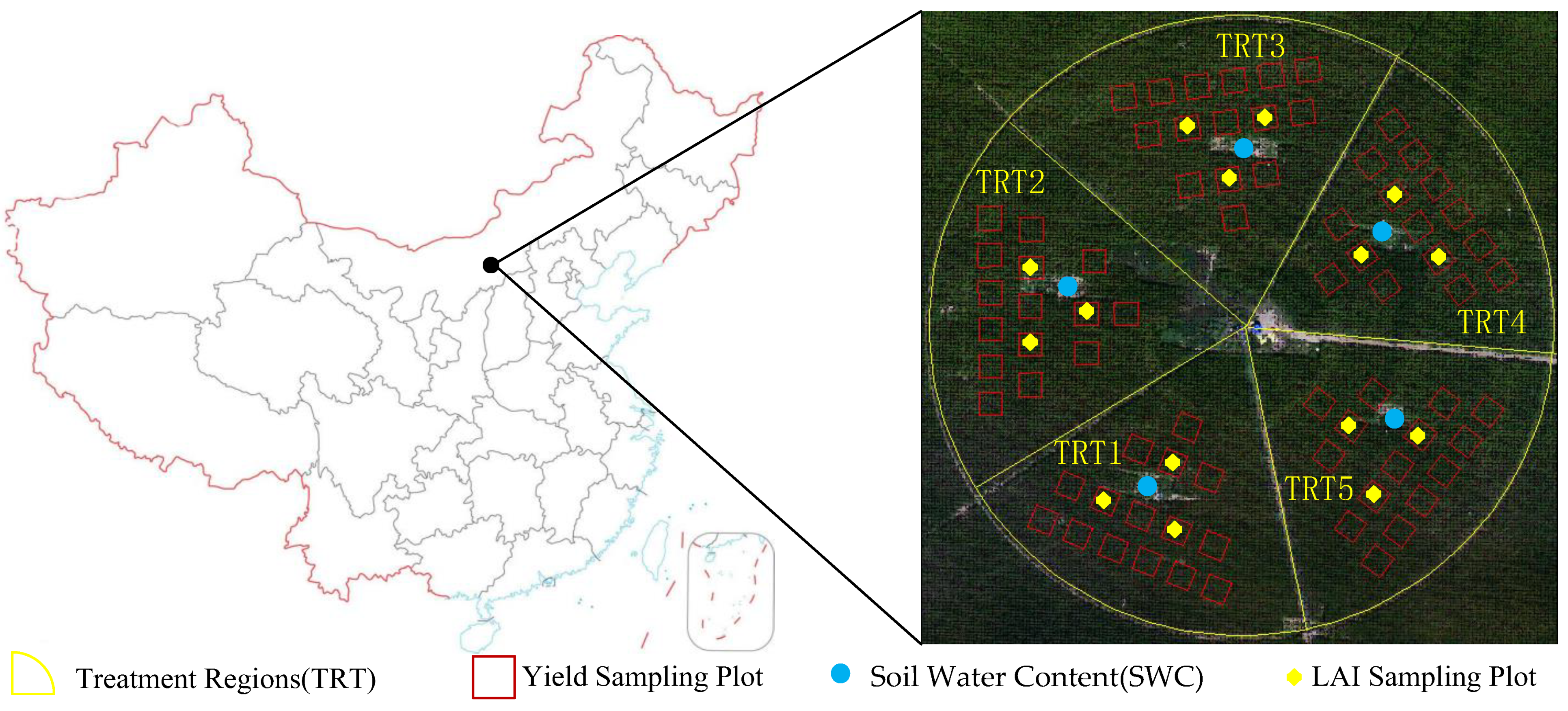
This study was conducted in a 1.13 ha research field (40°26′0.29″N, 109°36′25.99″E; elevation: 1010 m), located in Zhaojun Town, Dalate Banner, Ordos, Inner Mongolia, China. The study area was divided into five different water treatment zones (TRTs). Each TRT had 15 sampling plots, with an area of 3 × 3 m2. Three LAI sampling plots were selected for data collection in each experimental area, as shown in Figure 1. The field moisture capacity was measured at different depths using the cutting ring method. The field moisture capacity (volumetric) of soil samples with sampling depths of 30, 60, and 90cm were 20.3, 22.4 and 24.2%, respectively. At the effective rooting depth (0–90 cm), the average field moisture capacity (volumetric) of soil was 23%. The average permanent wilting point of soil profile was 5.6% (volume) and the bulk density was 1.56 g·cm−3. Other soil characteristics were estimated using mixed soil samples in 30, 60 and 90cm layers. According to the USDA Soil Classification, the soil type is loamy sand (80.7% sand, 13.7% silt, and 5.6% clay). The soil pH was 9.27, the organic matter content was 47.17 g/kg, and the C content was 27.35 g/kg. Corn (Junkai 918) was sown on May 4, 2019 (DOY, Day of Year, 124) with a row spacing of 0.58 m and a plant spacing of 0.25 m, with a row direction of east to west. The corn sprouted on May 11, 2019, was harvested on September 10, and had a life span of 122 days.
The study was divided into five processing regions (Figure 1). Calculation of irrigation was based on the evaporation and transpiration (ET). The crop coefficient method and FAO-56 were used to calculate ET [53]. The total amount of irrigation in late vegetative, reproductive and mature stages of the crop was 250 mm. Among them, TRT1 was fully irrigated, with a total irrigation amount of 256.2 mm. In this study, the control variable method was adopted for deficit irrigation. Different TRTs were subjected to different levels of deficit irrigation in the late vegetative and reproductive stages. Therefore, the percentage of water depth applied to different degrees of deficit irrigation is described for TRT1 crops in the late vegetative and reproductive stages. For example, the applied water depth of TRT 4 was 74% at the end of the vegetation period (Table 1).
2.2. Field Data Collection
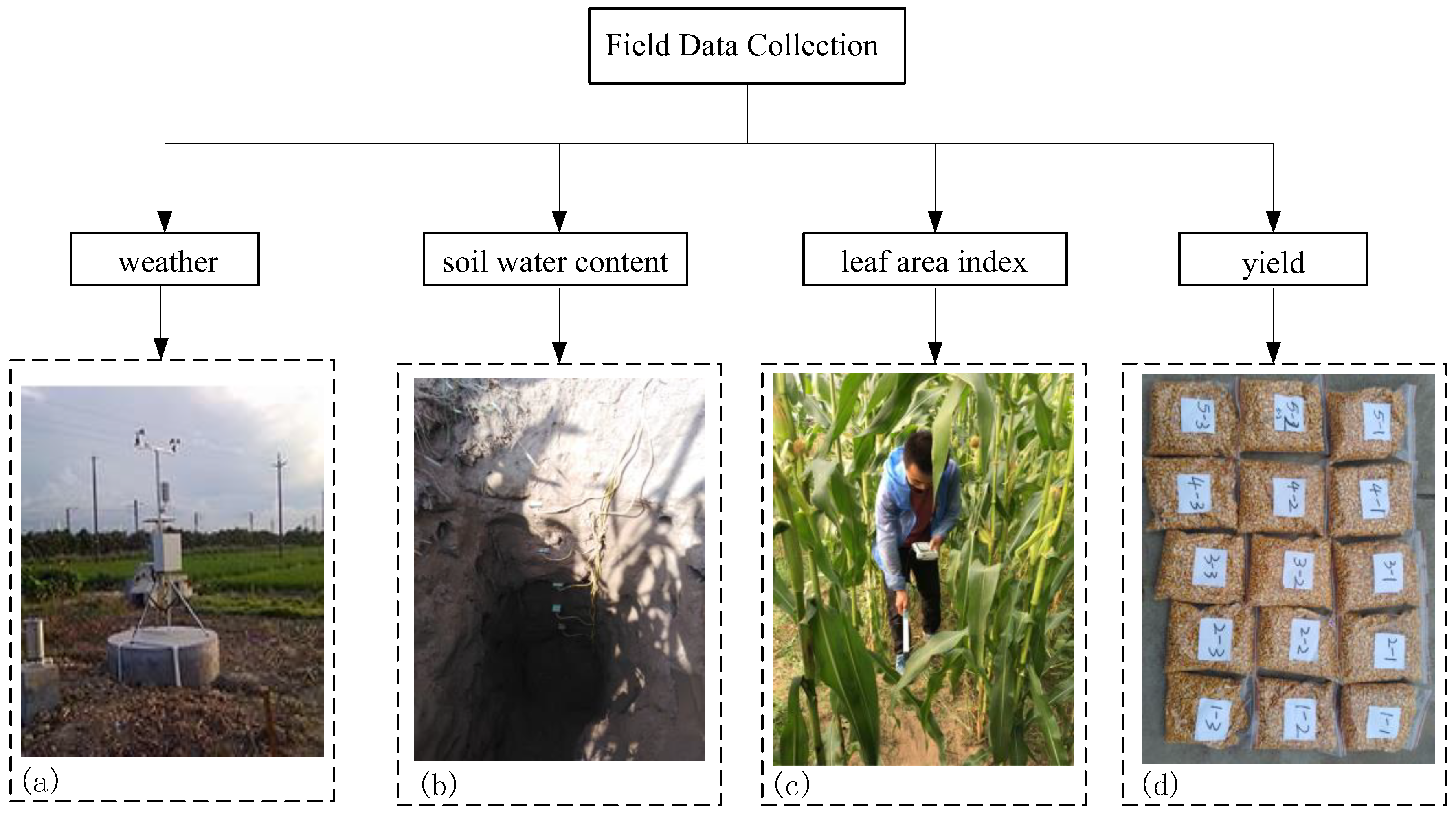
Figure 2 shows the field data collection, including weather (Figure 2a), soil water content (SWC, Figure 2b), leaf area index (LAI, Figure 2c), and yield (Figure 2d). Crop growth model simulations require daily weather observations and soil water characteristics. The weather variables include daily solar radiation, precipitation, and maximum/minimum/mean temperature. Weather data were collected from surface weather stations. SWC was measured by using TDR-315L (Acclima, USA) at the center of each TRT (Figure 1). The soil profile was divided into six layers, with depths of 10, 25, 50, 100, 120, and 150 cm, and each layer had a time domain reflectometer (TDR).
The maize biological parameters of LAI were measured before sunset for 2 h in order to avoid the influence of direct sunlight. The time to collect UAV data is the same as the time to collect LAI. There are three LAI sampling points in each TRT (Figure 1). A total of 15 sets of samples (LAI) were obtained per day. LAI was measured by using LAI-2000C (LI-COR, USA). The upper side of fully sunlit leaves was chosen to perform three repeated measurements at each sample site. At each sampling site, the radiation value was first measured at the top of canopy, and then at four marking points under the canopy.
The 75 sampling plots were all harvested on 10 September 2019. In each plot, all of the aboveground plant materials (around 9 m2) were cut for destructive measurements of final yield. The harvested materials were exposed to the sun for 10 days before the seed was threshed. The seeds were then cleaned and put into an oven at 80 °C until their weights did not change (after around four days). All the dry seeds were weighed together and the plot yield was calculated as the ratio of this total weight to the ground area (kg/ha).
2.3. UAV Camera System for Multispectral Imagery and Data Collection
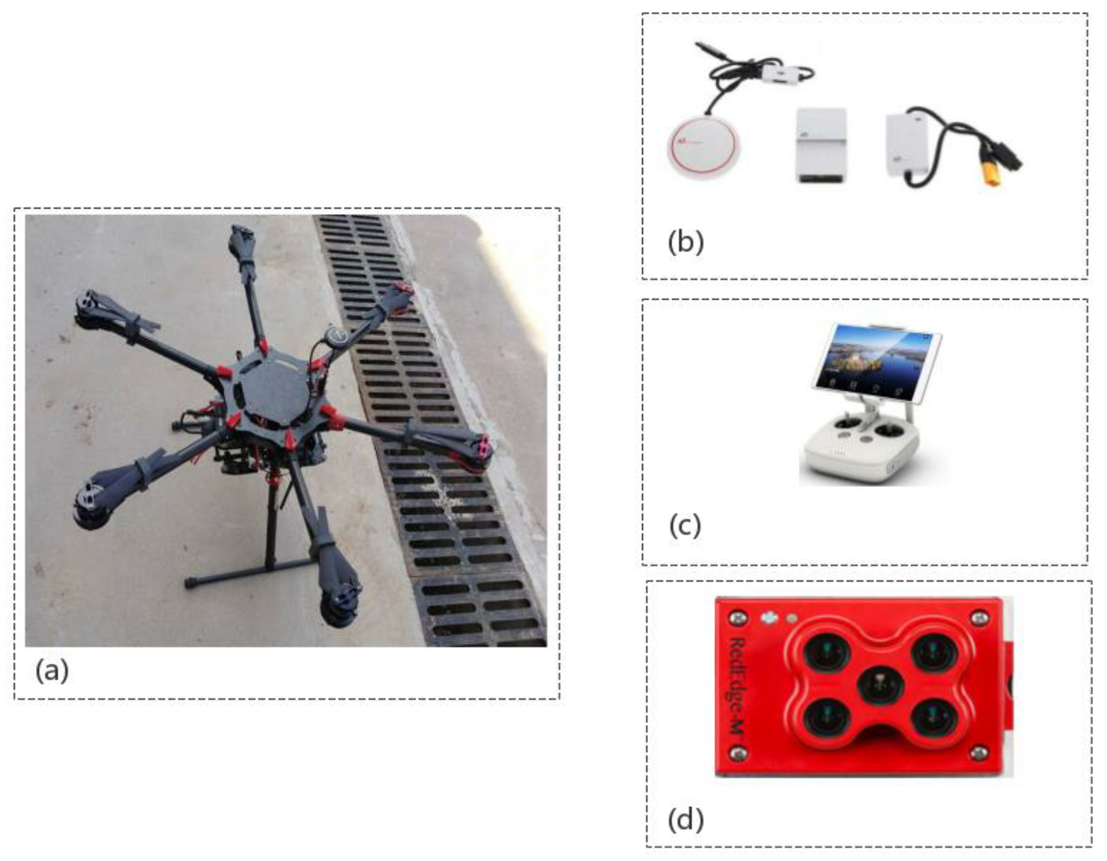
In this work, a commercial aircraft DJI Spreading Wings S1000 Multirotor UAV (DJI Company, Shenzhen, China) and a five-band multispectral camera (RedEdge, MicaSense Inc., Seattle, WA, USA), as displayed in Figure 3, constituted the platform of a low-altitude UAV camera system. The diameter, height, take-off weight, and hovering time of DJI S1000 were 1045 mm, 386 mm, 6.0 kg, 11.0 kg and 30 min, respectively. The weight, dimensions and image resolution of the RedEdge camera were 135 g, 5.9 cm 4.1 cm 3.0 cm and 1280 × 960 pixels, respectively. The RedEdge camera, equipped with GPS, can capture five spectral images simultaneously, where the spectral information is displayed in Table 2. Multispectral images were acquired at several key maize developmental stages including vegetative stages and reproductive stages (01 July 2019, 12 July 2019, 20 July 2019, 7 August 2019, 12 August 2019, 25 August 2019, 4 September 2019), respectively.
During each flight, the RedEdge camera was mounted on the gimbal and pointed vertically downwards to ensure aerial image quality. The flight was set at an altitude of 70 m above the ground, providing images with spatial resolutions of 5.5 cm/pixel on the ground. An iPad with a remote control was used to plan, monitor and control drone flights. The flight path was planned, and speed and camera triggers were designed so as to obtain continuous images with overlaps and side overlaps of up to 75% for accurate generation. The image was calibrated with a standard reflectivity black and white cloth. Each UAV aerial image contains information needed for camera calibration and image stitching, such as camera information (e.g., exposure time, ISO speed, focal length, and black level), GPS, and IMU (e.g., latitude, longitude, altitude, yaw, pitch, and roll).
Pix4DMapper software (commercial version 4.2.27) was used for image preprocessing to generate corrected and geo-referenced spectral reflectance, including initial processing, conformal generation and exponential calculation (with reflectance correction). The output of each layer was a single high-resolution TIFF image. The TIFF image was further postprocessed in MATLAB to determine the sample map of each image layer for subsequent analysis.
2.4. Crop Growth Model
In the data assimilation framework, we used a modified version of the SAFY model [32]. SAFY is a simple crop growth simulation model that has been successfully applied to evaluate crop growth and yield for maize, wheat and soybeans [54,55,56]. This model can well summarize the biomass accumulation, allocation and phenology. Compared to popular crop growth models such as DSSAT and WOFOST, SAFY has few free parameters to specify, which makes it attractive for large-area practical applications. It also allows investigations to understand the feedback between ENKF and crop model behavior.
In SAFY, the aboveground dry biomass production is driven by incoming photosynthetically active radiation (PAR) and constrained by air temperature. Two phenological stages (vegetative and grain) controlled the allocation of accumulated carbon to leaves and grains. The environmental stress of crops was compensated for by the field-specific effective light use efficiency (ELUE) parameter. Water stress is an important factor limiting crop yield. Therefore, in this study, we used soil water content (SWC) to simulate the crop water stress dynamics. The crop water stress coefficient was calculated by SWC, and SWC was measured by the time domain reflectometry (TDR) soil moisture sensor. Finally, the crop water stress coefficient (calculated as a ratio of actual transpiration to potential transpiration) decreased the daily accumulation of new biomass in primary growth modules accordingly.
The modified SAFY model, hereafter referred to as SAFYswc, has six free parameters: the day of emergence (D0 ), ELUE, and four coefficients (PLa, PLb, SenA, and SenB) describing the crop phenological stages (Table 3) as reported in the original SAFYswc paper [32]. The four phenological parameters are related to the genetic characters of specific crop type and cultivar, while the emergence day and ELUE are dependent on the environment. Other parameters, such as those related to soil water dynamics and temperature stress are assumed to be constant (Table 3). Our decisions of which parameters to fix and which to free were based on a number of previous studies [6,55,57]. The SAFYswc model was calibrated and validated using the long-term crop observations in official government data (2008–2018) to make sure the simulations matched the observations of the biomass, LAI and soil moisture, and evapotranspiration.
2.5. Data Assimilation and Technical Processes
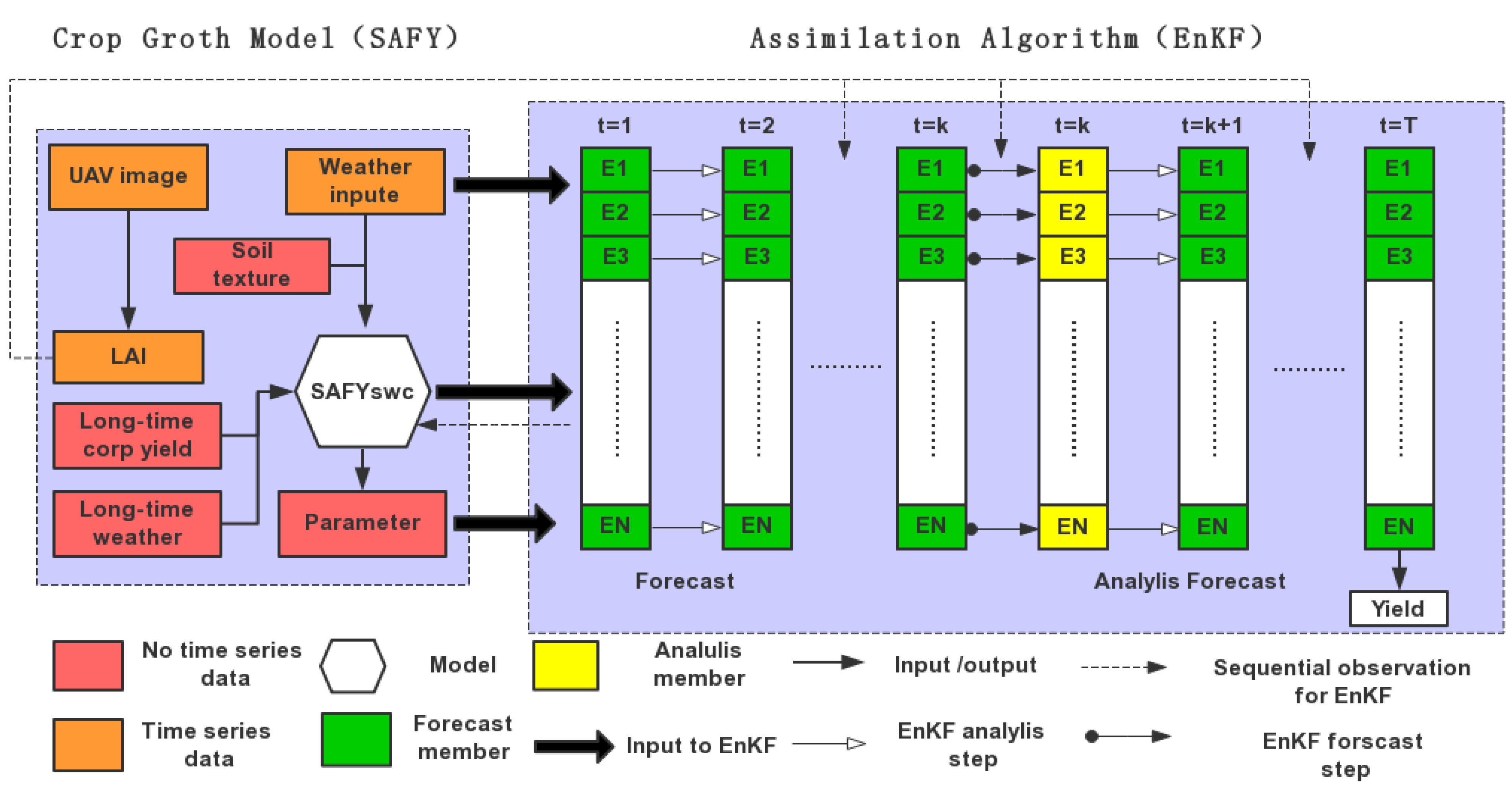
In this study, the data assimilation method adopted is the Ensemble Kalman Filter (EnKF). The Kalman filter is an analytic solution to the general state estimation problem defined by data assimilation, where two complementary sources of information simulations and observations are synthesized to provide a better estimate that has no bias and minimum variance. The Kalman filter recursively estimates the model states with a step followed by an analysis step. In the forecast step, model states and error covariance evolve over time without interruption.
As shown in Figure 4, on the left is the model recalibration phase. On the right is the EnKF data assimilation phase at the field level. On the left, it also tells how SAFYswc works. SAFY is driven by meteorological data and simulates the growth process of crops in steps by day. UAV remote sensing images were used as modified data in the simulation of the crop model. Ei is the forecast and analysis state vectors for ensemble member i. N is the total number of ensemble members. There are a total of T time steps. At the different forecast steps, each ensemble member propagates independently using SAFYswc and the parameter set. When an observation of LAI is available, the ensemble stops propagating and performs the analysis step that updates the simulated LAI (analysis step).
2.6. Vegetation Index Calculation and Model Evaluation
In this study, four models were tested for LAI estimation using canopy reflectance data. VI is the transformations of two or more reflectance bands to enhance the vegetation features. The VIs tested in this study are summarized in Table 4. The 105 samples were divided into a training set and a verification set. The training set is 70, and the verification set is 35. The coefficient of determination (R2) and the root mean square error (RMSE) were used to evaluate the model fit.
3. Result
3.1. LAI Estimation Using Vegetation Indices
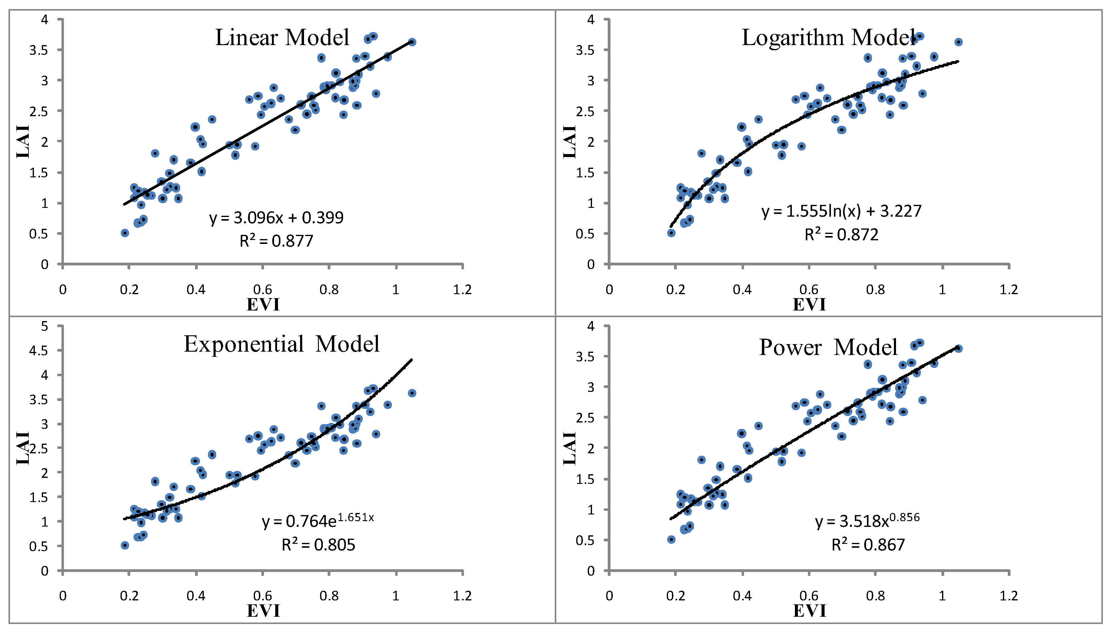
In this work, data from two sample plots (70 groups) in each TRT were selected for modeling, and data from the other sample plot (35 groups) in each TRT were selected for verification. LAI was the only observation to be assimilated into the SAFYswc model. Therefore, the important step is to estimate LAI using remotely sensed data for remote prediction of yield. Some widely used Vis (Table 4), obtained from UAV cameras, are related to LAI measurements. The vegetation index was taken as the independent variable and the leaf area index as the dependent variable. The linear model, exponential model, logarithmic model and quadratic polynomial model were constructed, and the optimal model was selected as the estimation model of leaf area index. The optimal estimation model of LAI inversion regression equation is shown in Table 5.
There was a significant regression relationship between most vegetation indices and leaf area indices. The regression equation R2 of each model was estimated to be greater than 0.724, which reached significance. Among all the indexes involved in this experiment, the inversion results, from high to low, are EVI, NDVI, OSAVI, GNDVI, MSAVI2, and EVI2. The regression model of leaf area index estimation equation based on EVI2 has a lower determination coefficient R2=0.724. The estimation model and validation results of LAI are shown in Figure 5. The R2 of the four models based on EVI inversion LAI were all higher than 0.8. The leaf area index model was inverted by EVI with the highest determination coefficient (R2 = 0.877).
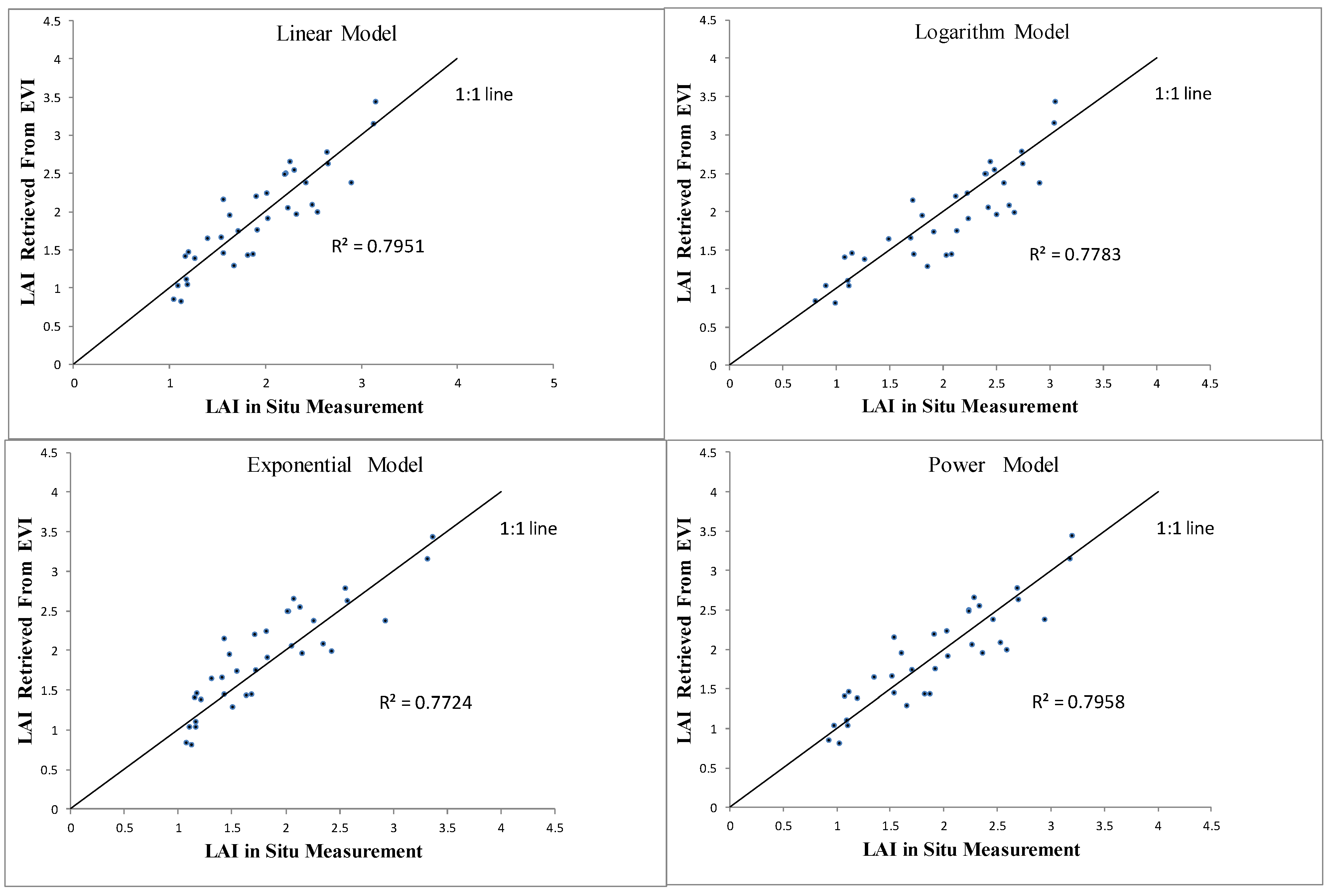
The validation accuracy of the LAI inversion model constructed by EVI is also generally high, with a maximum R2 of 0.795 (Figure 6). In conclusion, LAI inversion accuracy based on vegetation index EVI and a linear model is the highest. EVI has the highest inversion accuracy and the best verification effect, so EVI is selected as the inversion index of LAI.
3.2. Comparison of Observation Yield and Estimated Yield
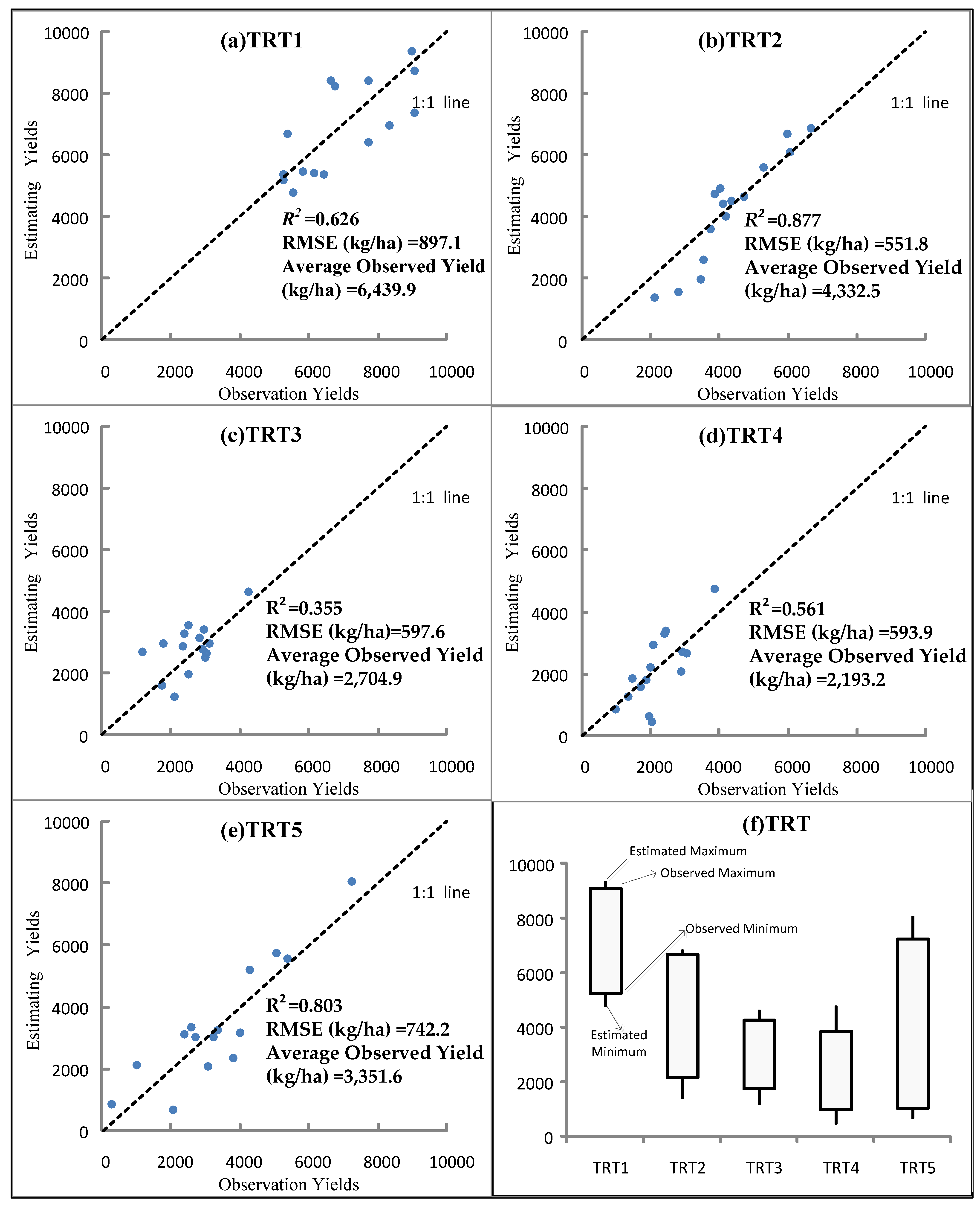
The yield of crops is greatly affected by water. The yields of crops in different irrigation treatment regions vary greatly, as shown in Figure 7. The highest average yield of the treatment region (TRT1) was 6439.9 kg/ha. The lowest average yield of the treatment region (TRT4) was 2193.2 kg/ha. The estimation accuracy of different treatment regions is also different. Among them, the highest estimation accuracy is TRT2, whose R2 is 0.877. The lowest estimated accuracy is TRT3, whose R2 is only 0.355. The applied water depth, from high to low, is TRT1, TRT2, TRT5, TRT3, and TRT4. The estimated yield accuracy, from high to low is TRT2, TRT5, TRT1, TRT4, and TRT3. As shown in Figure 7, treatment regions with moderate water deficit (TRT2 and TRT5) have the highest accuracy when estimating yield. The yield estimation accuracy is poor in treatment regions with saturated irrigation (TRT1). However, the yield estimation accuracy for severe deficit irrigation (TRT3 and TRT4) was the lowest.
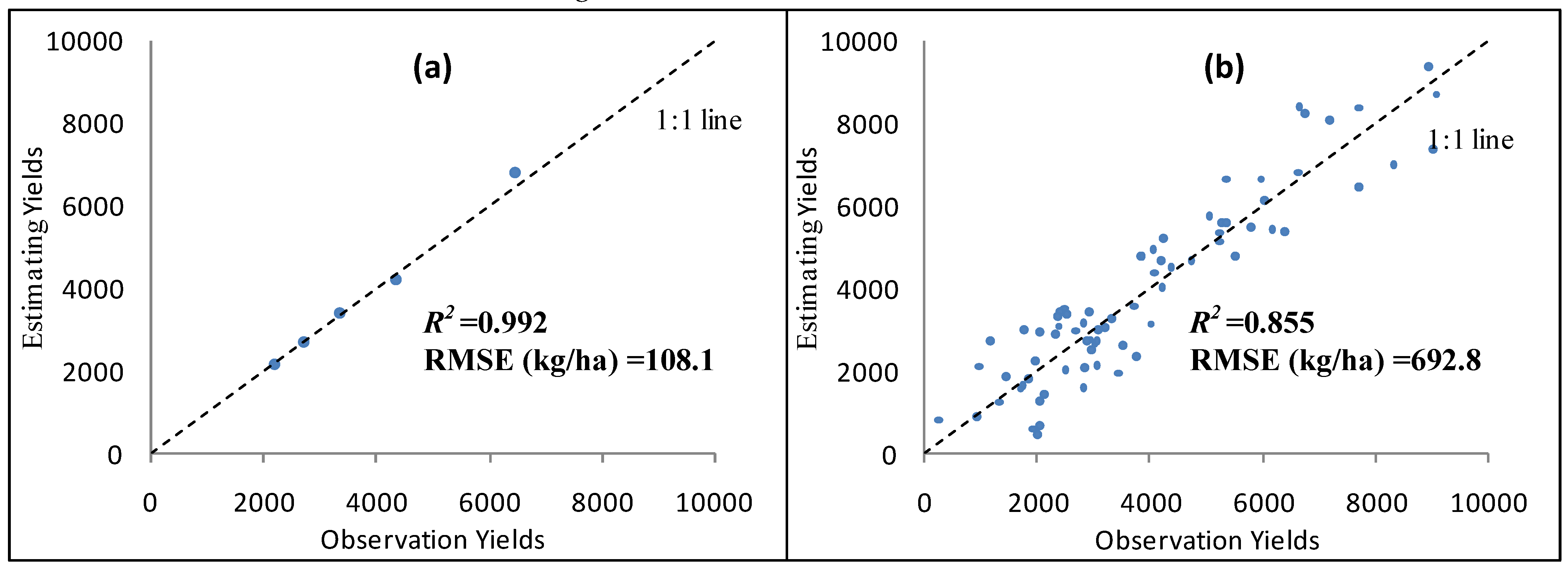
Figure 7f shows the maximum/minimum of the observed yield and the maximum/minimum of the estimated yield. The yield distribution gradient of moderate deficit irrigation is large. The yield distribution gradient of severe deficit irrigation is small. This may be due to the spatial heterogeneity of soil water content. The spatial heterogeneity of soil water content includes the imbalance of soil water holding capacity and soil fertility in different places. Under the conditions of saturated irrigation and severe deficit irrigation, the spatial heterogeneity of soil water content was not obvious. However, under moderate water deficit, the imbalance of spatial heterogeneity of soil water content was obvious. We used different irrigation treatments for different experimental areas. Yield gradients were higher in different irrigation treatments than in natural conditions. The applicability of this method can be better examined with a high yield gradient. Soil imbalance can lead to different crop yields at the same level of irrigation. Under different irrigation levels, the imbalance of soil will aggravate the difference of yield. As shown in Figure 8, we compared the measured and estimated average yields at five different irrigation levels. The measured average yield and the estimated average yield at five different irrigation levels were basically the same. We compared the observed and estimated yields at all sample points and at five different irrigation levels. As shown in Figure 8, the yield estimation accuracy was generally good at different irrigation levels, with R2 = 0.855 and RMSE = 692.8 kg/ha.
3.3. Yield Mapping
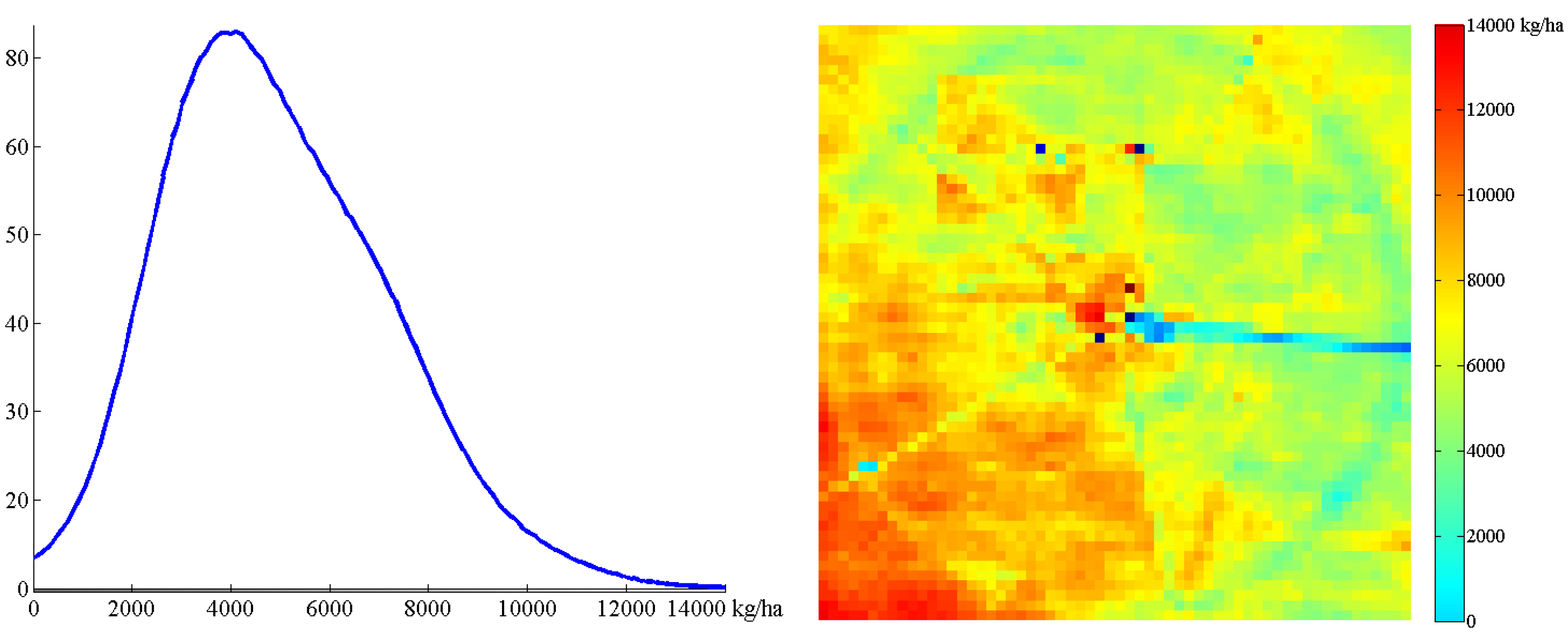
At different growth stages, we took multispectral images with 5 cm spatial resolution. If we used data assimilation at 5 cm spatial distribution, the computational burden would become huge. In order to get a better sense of the mapped maize yield with data assimilation, we obtained the yield estimate mapping at 2 m spatial resolution. We compared the distributions of yield estimated by the data assimilation approach with different levels of irrigation (Figure 9). The yield (data assimilation) ranged from 2000 to 10,000 kg/ha. Different irrigation treatments result in a larger yield gradient, which is well represented in the yield histogram. Water is the main factor affecting yield. The effect of water on yield can be clearly seen from the figure. With the help of spatially explicit LAI input, the data assimilation yield estimates present both between- and within-field variability.
4. Discussion
4.1. Accuracy of LAI Inversion and its Influence on Yield Estimation Accuracy
Compared with DASST and WOFOST, SAFY is relatively simple. Therefore, SAFY has a poor capability of correcting LAI. The accuracy of yield estimation by SAFY and LAI through data assimilation depends on the inversion accuracy of LAI. Moreover, in the late growth stage of crops, there will be a phenomenon of vegetation supersaturation. This will lead to a decrease in the accuracy of LAI inversion for crops. Especially in the linear model, the actual LAI of crops would be higher than the inversion LAI. This will affect the accuracy of production estimation. To solve this problem, LAI inversion can be changed from single multispectral image inversion to multisource remote sensing inversion. Inversions can also be carried out through nonlinear models. The influence of vegetation supersaturation on inversion accuracy should be minimized.
4.2. Uncertainties in the Estimated Crop Yield
Figure 7 shows the difference between observed and estimated yields. During the experiment, no pests or diseases were found in the experimental area. Therefore, crop yield is mainly affected by temperature, soil water content, and nutrients. LAI is the only variable assimilated by remote sensing data and crop models. The main factor affecting crop yield estimation may be the estimation accuracy of LAI. Especially in the fully irrigated experimental area (TRT1), the low estimation accuracy is mainly due to the phenomenon of supersaturation in the later growth stage of maize.
The spatial heterogeneity of soil water content can also affect the accuracy of the experiment. The spatial heterogeneity of soil water content may be the main factor affecting the accuracy of the deficit irrigation experiment area. The treatment areas with different irrigation levels are adjacent to each other, and the different soil water content will cause a difference in the water potential. Horizontal water movement can be caused by water potential difference. There is only one measuring point of SWC in each TRT. In this study, the measuring points of SWC are not sufficient to represent the spatial heterogeneity of soil water content. Increasing the number of SWC measurement points can improve the accuracy of estimation. However, this is costly and difficult to carry out in actual production. In the future, remote sensing can be used to measure soil moisture.
The higher the resolution of yield estimation, the greater the influence of random error of soil equilibrium on the accuracy of yield estimation. As shown in Figure 8a, the accuracy of the yield estimate is greatly improved by lowering the resolution of the yield estimate. In the future, the accuracy of production estimation can be improved by appropriately reducing the resolution of production estimation.
In addition, the defects of the SAFY model itself also affect the results. SAFY is a relatively simple crop model, that only considers soil water content and temperature stress. The method of yield estimation based on multispectral effects and coupling of crop models can effectively show the imbalance. It can provide some guidance for precision agriculture. However, in the case of saturated irrigation and severe water deficits, which may be caused by the mechanism of the crop model itself, the applicability of the model still needs to be improved. In the future, we can improve the yield estimation accuracy by further improving the relevant modules of the crop model.
4.3. Yield Estimation and Data Assimilation
The empirical model is the simplest and most common way to estimate yield. Maimaitijiang et al. used machine learning to estimate soybean yield [58]. The objective of this study was to evaluate the power of UAV-based multimodal data fusion using RGB, multispectral, and thermal sensors to estimate soybean (Glycine max) grain yield within the framework of a Deep Neural Network (DNN). However, empirical models lack physiological explanations for crops, and the generalizability of the models is often poor. There have been successful operational applications using data assimilation and crop growth models such as DSSAT for crop yield estimation [49,59]. Yanghui et al. estimated crop yield, at the county scale, by using satellite remote sensing and the SAYF model [60]. This method was validated by multiple field-level maize yield datasets across major production states in the US Midwest. However, most studies have focused on district or regional level crop yield forecasting, likely due to a lack of robust high-resolution LAI (or other state variables) retrievals and field-level validation data. This work reduces the research area to the farmland scale and makes more accurate yield estimations through high-resolution LAI and accurate and controllable field data. The accuracy of this study is significantly improved compared to large-scale production estimates based on satellite remote sensing. The principle of this research is similar to that of Song et al. [15]. Crop models detail the complex interactions between environmental factors and management practices, but they also require clear information about soil characteristics and weather variables, as well as specific breed parameters that are difficult to obtain at a large scale, making them unusable for large-scale yield estimation applications. Most previous studies have used complex crop growth models, such as DSSAT and WOFOST, for data assimilation to estimate yields [61,62]. When data assimilation is applied, LAI is the only correction quantity, but complex models are less affected by LAI correction. For this reason, simpler crop models such as SAFY can be a better choice at the field scale.
5. Conclusions
In this paper, we assimilated remote sensing data from UAVs into crop models to effectively estimate corn yield at the farmland scale. In this study, we developed a method to estimate corn yield based on remote sensing data and ground monitoring data under different water treatments. We chose five common vegetation indexes to estimate the LAI inversion based on UAV vegetation index. A linear model, exponential model, logarithmic model, and quadratic polynomial model were constructed. Furthermore, the optimal model was selected as the estimation model of leaf area index. The study found that LAI inversion based on EVI vegetation index and linear model had the highest accuracy, where R2 and RMSE are 0.877 and 0.609, respectively. Maize yield estimation based on UAV remote sensing data and SAFY crop model data assimilation had different yield estimation accuracy under different water treatments. Generally, the higher the water stress, the lower the estimation accuracy. Moreover, the estimated yield is often higher than the observed yield in the treatment area with severe water stress. This method can be used to estimate corn yield, where R2 is 0.855 and RMSE is 692.8kg/ha. We also performed yield estimate mapping at 2 m spatial resolution, which offered higher spatial resolution and accuracy than satellite remote sensing. The great potential of UAV observations incorporated in crop data to monitor crop yield and improve agricultural management is therefore indicated.
Author Contributions
Conceptualization, X.P. and W.H.; Data curation, X.P. and J.A.; Formal analysis, X.P.; Investigation, X.P., J.A., and Y.W.; Writing—original draft, X.P.; Writing—review and editing, W.H., J.A., and Y.W. All authors have read and agreed to the published version of the manuscript.
Funding
This study was supported by the National Natural Science Foundation of China (51979233), the National Key R&D plan of the Ministry of Science and Technology of the People’s Republic of China (2017YFC0403203), and the 111 Project (No. B12007).
Data Availability Statement
Not applicable.
Acknowledgments
We would like to thank Mengfei Zhang, Jiandong Tang, and Chaoqun Li for their work on field data collection.
Conflicts of Interest
The authors declare no conflict of interest.
References
- Heimlich, R.; Sonka, S.; Khanna, M.; Lowenberg-DeBoer, J. Precision agriculture in the twenty-first century: Report of the National Research Council committee. Am. J. Agr. Econ. 1998, 80, 1159. [Google Scholar]
- Idso, S.B.; Jackson, R.D.; Reginato, R.J. Remote-Sensing of Crop Yields. Science 1977, 196, 19–25. [Google Scholar] [CrossRef]
- Liu, J.R.M.J.; Liu, J.; Miller, J.R.; Pattey, E.; Haboudane, D.; Strachan, I.B.; Hinther, M. Monitoring crop biomass accumulation using multi-temporal hyperspectral remote sensing data. In Proceedings of the 2004 IEEE International Geoscience and Remote Sensing Symposium, Anchorage, AK, USA, 20–24 September 2004; pp. 1637–1640. [Google Scholar] [CrossRef]
- Toscano, P.; Castrignanò, A.; Di Gennaro, S.F.; Vonella, A.V.; Ventrella, D.; Matese, A. A Precision Agriculture Approach for Durum Wheat Yield Assessment Using Remote Sensing Data and Yield Mapping. Agronomy 2019, 9, 437. [Google Scholar] [CrossRef] [Green Version]
- Shang, J.; Liu, J.; Poncos, V.; Geng, X.; Qian, B.; Chen, Q.; Dong, T.; Macdonald, D.; Martin, T.; Kovacs, J.; et al. Detection of Crop Seeding and Harvest through Analysis of Time-Series Sentinel-1 Interferometric SAR Data. Remote Sens. 2020, 12, 1551. [Google Scholar] [CrossRef]
- Dong, T.; Liu, J.; Qian, B.; Zhao, T.; Jing, Q.; Geng, X.; Wang, J.; Huffman, T.; Shang, J. Estimating winter wheat biomass by assimilating leaf area index derived from fusion of Landsat-8 and MODIS data. Int. J. Appl. Earth Obs. Geoinf. 2016, 49, 63–74. [Google Scholar] [CrossRef]
- Dong, T.; Shang, J.; Liu, J.; Qian, B.; Jing, Q.; Ma, B.; Huffman, T.; Geng, X.; Sow, A.; Shi, Y.; et al. Using RapidEye imagery to identify within-field variability of crop growth and yield in Ontario, Canada. Precis. Agric. 2019, 20, 1231–1250. [Google Scholar] [CrossRef]
- Shang, J.; Liu, J.; Ma, B.; Zhao, T.; Jiao, X.; Geng, X.; Huffman, T.; Kovacs, J.M.; Walters, D. Mapping spatial variability of crop growth conditions using RapidEye data in Northern Ontario, Canada. Remote Sens. Environ. 2015, 168, 113–125. [Google Scholar] [CrossRef]
- Rudorff, B.F.T.; Batista, G.T. Wheat yield estimation at the farm level using TM Landsat and agrometeorological data. Int. J. Remote Sens. 1991, 12, 2477–2484. [Google Scholar] [CrossRef]
- Ruwaimana, M.; Satyanarayana, B.; Otero, V.; Muslim, A.M.; Syafiq A, M.; Ibrahim, S.; Raymaekers, D.; Koedam, N.; Dahdouh-Guebas, F. The advantages of using drones over space-borne imagery in the mapping of mangrove forests. PLoS ONE 2018, 13, e0200288. [Google Scholar] [CrossRef] [PubMed] [Green Version]
- Duan, B.; Fang, S.H.; Zhu, R.S.; Wu, X.T.; Wang, S.Q.; Gong, Y.; Peng, Y. Remote Estimation of Rice Yield With Un-manned Aerial Vehicle (UAV) Data and Spectral Mixture Analysis. Front. Plant Sci. 2019, 10, 204. [Google Scholar] [CrossRef] [PubMed] [Green Version]
- Sagan, V.; Maimaitijiang, M.; Sidike, P.; Eblimit, K.; Peterson, K.T.; Hartling, S.; Esposito, F.; Khanal, K.; Newcomb, M.; Pauli, D.; et al. UAV-Based High Resolution Thermal Imaging for Vegetation Monitoring, and Plant Phenotyping Using ICI 8640 P, FLIR Vue Pro R 640, and thermoMap Cameras. Remote Sens. 2019, 11, 330. [Google Scholar] [CrossRef] [Green Version]
- Song, Y.; Wang, J. Winter Wheat Canopy Height Extraction from UAV-Based Point Cloud Data with a Moving Cuboid Filter. Remote Sens. 2019, 11, 1239. [Google Scholar] [CrossRef] [Green Version]
- Sanches, G.M.; Duft, D.G.; Kölln, O.T.; Luciano, A.C.D.S.; De Castro, S.G.Q.; Okuno, F.M.; Franco, H.C.J. The potential for RGB images obtained using unmanned aerial vehicle to assess and predict yield in sugarcane fields. Int. J. Remote Sens. 2018, 39, 5402–5414. [Google Scholar] [CrossRef]
- Song, Y.; Wang, J.; Shang, J.; Liao, C. Using UAV-Based SOPC Derived LAI and SAFY Model for Biomass and Yield Estimation of Winter Wheat. Remote Sens. 2020, 12, 2378. [Google Scholar] [CrossRef]
- Bansod, B.; Singh, R.; Thakur, R.; Singhal, G. A comparision between satellite based and drone based remote sensing technology to achieve sustainable development: A review. J. Agric. Environ. Int. Dev. 2017, 111, 383–407. [Google Scholar] [CrossRef]
- Zhang, C.; Kovacs, J.M. The application of small unmanned aerial systems for precision agriculture: A review. Precis. Agric. 2012, 13, 693–712. [Google Scholar] [CrossRef]
- Yao, X.; Wang, N.; Liu, Y.; Cheng, T.; Tian, Y.; Chen, Q.; Zhu, Y. Estimation of Wheat LAI at Middle to High Levels Using Unmanned Aerial Vehicle Narrowband Multispectral Imagery. Remote Sens. 2017, 9, 1304. [Google Scholar] [CrossRef] [Green Version]
- Hoffmann, H.; Jensen, R.; Thomsen, A.; Nieto, H.; Rasmussen, J.; Friborg, T. Crop water stress maps for an entire growing season from visible and thermal UAV imagery. Biogeosciences 2016, 13, 6545–6563. [Google Scholar] [CrossRef] [Green Version]
- Ferencz, C.; Bognár, P.; Lichtenberger, J.; Hamar, D.; Tarcsai, G.; Timár, G.; Molnár, G.; Pásztor, S.; Steinbach, P.; Székely, B.; et al. Crop yield estimation by satellite remote sensing. Int. J. Remote Sens. 2004, 25, 4113–4149. [Google Scholar] [CrossRef]
- Shang, J.; Liu, J.; Huffman, T.; Qian, B.; Pattey, E.; Wang, J.; Zhao, T.; Geng, X.; Kroetsch, D.; Dong, T.; et al. Estimating plant area index for monitoring crop growth dynamics using Landsat-8 and RapidEye images. J. Appl. Remote Sens. 2014, 8, 85196. [Google Scholar] [CrossRef] [Green Version]
- Hunt, J.E.R.; Hively, W.D.; Fujikawa, S.J.; Linden, D.S.; Daughtry, C.S.T.; Mccarty, G.W. Acquisition of NIR-Green-Blue Digital Photographs from Unmanned Aircraft for Crop Monitoring. Remote Sens. 2010, 2, 290–305. [Google Scholar] [CrossRef] [Green Version]
- Dong, T.; Liu, J.; Qian, B.; Jing, Q.; Croft, H.; Chen, J.; Wang, J.; Huffman, T.; Shang, J.; Chen, P. Deriving Maximum Light Use Efficiency From Crop Growth Model and Satellite Data to Improve Crop Biomass Estimation. IEEE J. Sel. Top. Appl. Earth Obs. Remote Sens. 2016, 10, 104–117. [Google Scholar] [CrossRef]
- Casanova, D.; Epema, G.; Goudriaan, J. Monitoring rice reflectance at field level for estimating biomass and LAI. Field Crop. Res. 1998, 55, 83–92. [Google Scholar] [CrossRef]
- Berni, J.A.J.; Zarco-Tejada, P.J.; Suarez, L.; Fereres, E. Thermal and Narrowband Multispectral Remote Sensing for Vegetation Monitoring From an Unmanned Aerial Vehicle. IEEE Trans. Geosci. Remote Sens. 2009, 47, 722–738. [Google Scholar] [CrossRef] [Green Version]
- Zhou, X.; Zheng, H.; Xu, X.; He, J.; Ge, X.; Yao, X.; Cheng, T.; Zhu, Y.; Cao, W.; Tian, Y. Predicting grain yield in rice using multi-temporal vegetation indices from UAV-based multispectral and digital imagery. ISPRS J. Photogramm. Remote Sens. 2017, 130, 246–255. [Google Scholar] [CrossRef]
- Kouadio, L.; Newlands, N.K.; Davidson, A.; Zhang, Y.; Chipanshi, A. Assessing the Performance of MODIS NDVI and EVI for Seasonal Crop Yield Forecasting at the Ecodistrict Scale. Remote Sens. 2014, 6, 10193–10214. [Google Scholar] [CrossRef] [Green Version]
- Peng, Y.; Zhu, T.; Li, Y.; Dai, C.; Fang, S.; Gong, Y.; Wu, X.; Zhu, R.; Liu, K. Remote prediction of yield based on LAI estimation in oilseed rape under different planting methods and nitrogen fertilizer applications. Agric. For. Meteorol. 2019, 271, 116–125. [Google Scholar] [CrossRef]
- Kim, N.; Ha, K.-J.; Park, N.-W.; Cho, J.; Hong, S.; Lee, Y.-W. A Comparison Between Major Artificial Intelligence Models for Crop Yield Prediction: Case Study of the Midwestern United States, 2006–2015. ISPRS Int. J. Geoinf. 2019, 8, 240. [Google Scholar] [CrossRef] [Green Version]
- Khaki, S.; Wang, L. Crop Yield Prediction Using Deep Neural Networks. Front. Plant Sci. 2019, 10, 621. [Google Scholar] [CrossRef] [Green Version]
- Cheng, Z.; Meng, J.; Wang, Y. Improving Spring Maize Yield Estimation at Field Scale by Assimilating Time-Series HJ-1 CCD Data into the WOFOST Model Using a New Method with Fast Algorithms. Remote Sens. 2016, 8, 303. [Google Scholar] [CrossRef] [Green Version]
- Duchemin, B.; Maisongrande, P.; Boulet, G.; Benhadj, I. A simple algorithm for yield estimates: Evaluation for semi-arid irrigated winter wheat monitored with green leaf area index. Environ. Model. Softw. 2008, 23, 876–892. [Google Scholar] [CrossRef] [Green Version]
- Brisson, N.; Gary, C.; Justes, E.; Roche, R.; Mary, B.; Ripoche, D.; Zimmer, D.; Sierra, J.; Bertuzzi, P.; Burger, P.; et al. An overview of the crop model stics. Eur. J. Agron. 2003, 18, 309–332. [Google Scholar] [CrossRef]
- Steduto, P.; Hsiao, T.C.; Raes, D.; Fereres, E. AquaCrop-The FAO Crop Model to Simulate Yield Response to Water: I. Concepts and Underlying Principles. Agron. J. 2009, 101, 426–437. [Google Scholar] [CrossRef] [Green Version]
- Monteith, J.L. Solar Radiation and Productivity in Tropical Ecosystems. J. Appl. Ecol. 1972, 9, 747. [Google Scholar] [CrossRef] [Green Version]
- Maas, S.J. Parameterized Model of Gramineous Crop Growth: I. Leaf Area and Dry Mass Simulation. Agron. J. 1993, 85, 348–353. [Google Scholar] [CrossRef]
- Zhang, C.; Liu, J.; Dong, T.; Shang, J.; Tang, M.; Zhao, L.; Cai, H. Evaluation of the Simple Algorithm for Yield Estimate Model in Winter Wheat Simulation under Different Irrigation Scenarios. Agron. J. 2019, 111, 2970–2980. [Google Scholar] [CrossRef]
- Zhang, C.; Liu, J.; Dong, T.; Pattey, E.; Shang, J.; Tang, M.; Cai, H.; Saddique, Q. Coupling Hyperspectral Remote Sensing Data with a Crop Model to Study Winter Wheat Water Demand. Remote Sens. 2019, 11, 1684. [Google Scholar] [CrossRef] [Green Version]
- Mariotto, I.; Thenkabail, P.S.; Huete, A.; Slonecker, E.T.; Platonov, A. Hyperspectral versus multispectral crop-productivity modeling and type discrimination for the HyspIRI mission. Remote Sens. Environ. 2013, 139, 291–305. [Google Scholar] [CrossRef]
- Johnson, D.M. An assessment of pre- and within-season remotely sensed variables for forecasting corn and soybean yields in the United States. Remote Sens. Environ. 2014, 141, 116–128. [Google Scholar] [CrossRef]
- Zaman-Allah, M.; Vergara, O.; Araus, J.L.; Tarekegne, A.; Magorokosho, C.; Zarco-Tejada, P.J.; Hornero, A.; Albà, A.H.; Das, B.; Craufurd, P.Q.; et al. Unmanned aerial platform-based multi-spectral imaging for field phenotyping of maize. Plant Methods 2015, 11, 1–10. [Google Scholar] [CrossRef] [PubMed] [Green Version]
- Wang, K.; Franklin, S.E.; Guo, X.; Cattet, M. Remote Sensing of Ecology, Biodiversity and Conservation: A Review from the Perspective of Remote Sensing Specialists. Sensors 2010, 10, 9647–9667. [Google Scholar] [CrossRef]
- Sidike, P.; Asari, V.K.; Sagan, V. Progressively Expanded Neural Network (PEN Net) for hyperspectral image classification: A new neural network paradigm for remote sensing image analysis. ISPRS J. Photogramm. Remote Sens. 2018, 146, 161–181. [Google Scholar] [CrossRef]
- Colomina, I.; Molina, P. Unmanned aerial systems for photogrammetry and remote sensing: A review. ISPRS J. Photogramm. Remote Sens. 2014, 92, 79–97. [Google Scholar] [CrossRef] [Green Version]
- Maimaitijiang, M.; Ghulam, A.; Sidike, P.; Hartling, S.; Maimaitiyiming, M.; Peterson, K.; Shavers, E.; Fishman, J.; Peterson, J.; Kadam, S.; et al. Unmanned Aerial System (UAS)-based phenotyping of soybean using multi-sensor data fusion and extreme learning machine. ISPRS J. Photogramm. Remote Sens. 2017, 134, 43–58. [Google Scholar] [CrossRef]
- Maresma, Á.; Ariza, M.; Martinez, E.; Lloveras, J.; Martínez-Casasnovas, J.A. Analysis of Vegetation Indices to Determine Nitrogen Application and Yield Prediction in Maize (Zea mays L.) from a Standard UAV Service. Remote Sens. 2016, 8, 973. [Google Scholar] [CrossRef] [Green Version]
- Zhao, Y.; Chen, S.; Shen, S. Assimilating remote sensing information with crop model using Ensemble Kalman Filter for improving LAI monitoring and yield estimation. Ecol. Model. 2013, 270, 30–42. [Google Scholar] [CrossRef]
- Li, Y.; Zhou, Q.; Zhou, J.; Zhang, G.; Chen, C.; Wang, J. Assimilating remote sensing information into a coupled hydrology-crop growth model to estimate regional maize yield in arid regions. Ecol. Model. 2014, 291, 15–27. [Google Scholar] [CrossRef]
- Ines, A.V.; Das, N.N.; Hansen, J.W.; Njoku, E.G. Assimilation of remotely sensed soil moisture and vegetation with a crop simulation model for maize yield prediction. Remote Sens. Environ. 2013, 138, 149–164. [Google Scholar] [CrossRef] [Green Version]
- Sakov, P.; Oke, P.R. A deterministic formulation of the ensemble Kalman filter: An alternative to ensemble square root filters. Tellus A: Dyn. Meteorol. Oceanogr. 2008, 60, 361–371. [Google Scholar] [CrossRef] [Green Version]
- Pauwels, V.R.N.; Verhoest, N.E.C.; De Lannoy, G.J.M.; Guissard, V.; Lucau, C.; Defourny, P. Optimization of a coupled hydrology-crop growth model through the assimilation of observed soil moisture and leaf area index values using an ensemble Kalman filter. Water Resour. Res. 2007, 43, 1637–1640. [Google Scholar] [CrossRef] [Green Version]
- de Wit, A.; van Diepen, C. Crop model data assimilation with the Ensemble Kalman filter for improving regional crop yield forecasts. Agric. For. Meteorol. 2007, 146, 38–56. [Google Scholar] [CrossRef]
- Tang, J.; Han, W.; Zhang, L. UAV Multispectral Imagery Combined with the FAO-56 Dual Approach for Maize Evapotranspiration Mapping in the North China Plain. Remote Sens. 2019, 11, 2519. [Google Scholar] [CrossRef] [Green Version]
- Silvestro, P.C.; Pignatti, S.; Yang, H.; Yang, G.; Pascucci, S.; Castaldi, F.; Casa, R. Sensitivity analysis of the Aquacrop and SAFYE crop models for the assessment of water limited winter wheat yield in regional scale applications. PLoS ONE 2017, 12, e0187485. [Google Scholar] [CrossRef] [PubMed] [Green Version]
- Duchemin, B.; Fieuzal, R.; Rivera, M.A.; Ezzahar, J.; Jarlan, L.; Rodriguez, J.C.; Hagolle, O.; Watts, C. Impact of Sowing Date on Yield and Water Use Efficiency of Wheat Analyzed through Spatial Modeling and FORMOSAT-2 Images. Remote Sens. 2015, 7, 5951–5979. [Google Scholar] [CrossRef] [Green Version]
- Battude, M.; Al Bitar, A.; Morin, D.; Cros, J.; Huc, M.; Sicre, C.M.; Le Dantec, V.; Demarez, V. Estimating maize biomass and yield over large areas using high spatial and temporal resolution Sentinel-2 like remote sensing data. Remote Sens. Environ. 2016, 184, 668–681. [Google Scholar] [CrossRef]
- Betbeder, J.; Fieuzal, R.; Baup, F. Assimilation of LAI and Dry Biomass Data from Optical and SAR Images Into an Agro-Meteorological Model to Estimate Soybean Yield. IEEE J. Sel. Top. Appl. Earth Obs. Remote Sens. 2016, 9, 2540–2553. [Google Scholar] [CrossRef]
- Maimaitijiang, M.; Sagan, V.; Sidike, P.; Hartling, S.; Esposito, F.; Fritschi, F.B. Soybean yield prediction from UAV using multimodal data fusion and deep learning. Remote Sens. Environ. 2020, 237, 111599. [Google Scholar] [CrossRef]
- Andreadis, K.M.; Das, N.; Stampoulis, D.; Ines, A.; Fisher, J.B.; Granger, S.; Kawata, J.; Han, E.; Behrangi, A. The Regional Hydrologic Extremes Assessment System: A software framework for hydrologic modeling and data assimilation. PLoS ONE 2017, 12, e0176506. [Google Scholar] [CrossRef]
- Kang, Y.; Özdoğan, M. Field-level crop yield mapping with Landsat using a hierarchical data assimilation approach. Remote Sens. Environ. 2019, 228, 144–163. [Google Scholar] [CrossRef]
- Huang, J.; Sedano, F.; Huang, Y.; Ma, H.; Li, X.; Liang, S.; Tian, L.; Zhang, X.; Fan, J.; Wu, W. Assimilating a synthetic Kalman filter leaf area index series into the WOFOST model to improve regional winter wheat yield estimation. Agric. For. Meteorol. 2016, 216, 188–202. [Google Scholar] [CrossRef]
- Curnel, Y.; De Wit, A.J.; Duveiller, G.; Defourny, P. Potential performances of remotely sensed LAI assimilation in WOFOST model based on an OSS Experiment. Agric. For. Meteorol. 2011, 151, 1843–1855. [Google Scholar] [CrossRef]
Figure 1.
Aerial view of the experimental field indicating treatment region division and the location of sampling plots.
Figure 1.
Aerial view of the experimental field indicating treatment region division and the location of sampling plots.

Figure 2.
Schematic indicating the field data collection, including weather (a), soil water content (b), leaf area index (c), and yield (d).
Figure 2.
Schematic indicating the field data collection, including weather (a), soil water content (b), leaf area index (c), and yield (d).

Figure 3.
Unmanned aerial vehicle (UAV) camera system: DJI S800 UAV (a), Dji A3 flight controller (b), remote control (c) and RedEdge camera (d).
Figure 3.
Unmanned aerial vehicle (UAV) camera system: DJI S800 UAV (a), Dji A3 flight controller (b), remote control (c) and RedEdge camera (d).

Figure 4.
Schematic of the data assimilation and technical processes framework.

Figure 5.
The estimation model of LAI on EVI.

Figure 6.
The validation between the LAI retrieved from EVI and in situ measurements.

Figure 7.
Comparison between SAFY model estimated and in situ measurement of grain yield for five irrigation scenarios (a–e). The maximum/minimum of observed yield and the maximum/minimum of estimated yield (f).
Figure 7.
Comparison between SAFY model estimated and in situ measurement of grain yield for five irrigation scenarios (a–e). The maximum/minimum of observed yield and the maximum/minimum of estimated yield (f).

Figure 8.
Comparison of average grain yield between SAFY model estimated and situ measurement for five irrigation scenarios (a). Comparison of grain yield between SAFY model estimated and situ measurement (b).
Figure 8.
Comparison of average grain yield between SAFY model estimated and situ measurement for five irrigation scenarios (a). Comparison of grain yield between SAFY model estimated and situ measurement (b).

Figure 9.
The distributions of yield estimated by the data assimilation approach with sample data.


Table 1.
Experimental treatments and total applied water depth (percentage of full irrigation treatment in parentheses) which includes the amount of irrigation in the late vegetative, reproductive and maturation stages in 2019.
Table 1.
Experimental treatments and total applied water depth (percentage of full irrigation treatment in parentheses) which includes the amount of irrigation in the late vegetative, reproductive and maturation stages in 2019.
| Treatment | Applied Water Depth (mm) | |||
|---|---|---|---|---|
| Late Vegetative (07.04–07.27) | Reproductive (07.28–08.18) | Maturation (08.19–09.4) | Total | |
| TRT1 | 98.2 (100%) | 86.3 (100%) | 71.7 (100%) | 256.2 (100%) |
| TRT2 | 98.2 (100%) | 63.9 (74%) | 71.7 (100%) | 233.8 (91%) |
| TRT3 | 98.2 (100%) | 46.6 (54%) | 71.7 (100%) | 216.5 (85%) |
| TRT4 | 72.6 (74%) | 63.9 (74%) | 71.7 (100%) | 208.2 (81%) |
| TRT5 | 72.6 (74%) | 86.3 (100%) | 71.7 (100%). | 230.6 (90%) |
Table 2.
Spectral information of the RedEdge camera.
| Band No. | Name | Center Wavelength | Bandwidth | Panel Reflectance |
|---|---|---|---|---|
| 1 | Blue | 475 nm | 20 nm | 0.57 |
| 2 | Green | 560 nm | 20 nm | 0.57 |
| 3 | Red | 668 nm | 10 nm | 0.56 |
| 4 | NIR | 840 nm | 40 nm | 0.51 |
| 5 | RedEdge | 717 nm | 10 nm | 0.55 |
Table 3.
List of parameters and description for the modified simple algorithm for yield (SAFYswc) model.
Table 3.
List of parameters and description for the modified simple algorithm for yield (SAFYswc) model.
| Parameter | Description | Notation | Unit | Initial Value or Range a | |
|---|---|---|---|---|---|
| Fixed | Climatic efficiency | Ratio of incoming photosynthetically active radiation to global radiation | ε | - | 0.48 |
| Light-interception coefficient | Coefficient in Beer’s Law | K | - | 0.5 | |
| Optimal temperature for crop growth | The optimal temperature for crop functions | Topt | °C | 30 | |
| Minimum temperature for crop growth | The minimum temperature below which crop growth stops | Tmin | °C | 10 | |
| Maximum temperature for crop growth | The maximum temperature above which crop growth stops | Tmax | °C | 47 | |
| Specific leaf area | The ratio of leaf area to dry leaf mass | SLA | m2/g | 0.024 | |
| Initial aboveground biomass | The aboveground mass at emergence | DAM0 | g/m2 | 3.7 | |
| Root growth rate | Increase of root depth over time | Rgrt | cm·°C−1·Day−1 | 0.22 | |
| Root length/weight ratio | The ratio of root length to root dry weight | Rrt | cm/g | 0.98 | |
| Bare soil albedo | Albedo of bare soils | SALB | - | 0.16 | |
| Free | Day of Emergence | The day of the year when the dry biomass of the crop is 2.5 g/m2 | D0 | day | 120–160 |
| Leaf Partitioning Coefficient 1 | Initial fraction of daily accumulated dry biomass partitioned to leaf at the emergence | PLa | - | 0.1–0.4 | |
| Leaf Partitioning Coefficient 2 | PLa and PLb together determine the cumulated GDD when LAI reaches peak value | PLb | - | 0.001–0.01 | |
| Leaf Senescence Coefficient 1 | Cumulated GDD when leaf senescence starts (LAI decreases) | SenA | °C·Day | 500–1200 | |
| Leaf Senescence Coefficient 2 | Determines the rate of leaf senescence | SenB | °C·Day | 2000–15,000 | |
| Effective Light Use Efficiency | The ratio between produced dry biomass and APAR | ELUE | g/MJ | 2.5–5 | |
Table 4.
Vegetation indices used in this study.
| Vegetation Indices | Equation |
|---|---|
| Normalized difference vegetation index | NDVI = (NIR − R)/(NIR + R) |
| Optimized soil-adjusted vegetation index | OSAVI = (NIR − R)/(NIR + R + X) (x = 0.16) |
| Green normalized difference vegetation index | GNDVI = (NIR − G)/(NIR + G) |
| Enhanced vegetation index without a blue band | EVI2 = 2.5 (NIR − R)/(NIR + 2.4R + 1) |
| Modified secondary soil adjusted vegetation index | |
| Enhanced vegetation index | EVI = 2.5 (NIR − R)/(NIR + 6.0R − 7.5B + 1) |
Table 5.
The estimation and validation models of leaf area index (LAI) based on vegetation index.
| Vegetation Index | Optimal Model | Validation Models | ||
|---|---|---|---|---|
| R2 | RMSE | R2 | RMSE | |
| NDVI | 0.823 | 0.646 | 0.784 | 0.659 |
| OSAVI | 0.799 | 0.669 | 0.772 | 0.682 |
| GNDVI | 0.792 | 0.697 | 0.743 | 0.718 |
| EVI2 | 0.724 | 0.774 | 0.690 | 0.791 |
| MSAVI2 | 0.741 | 0.728 | 0.734 | 0.742 |
| EVI | 0.877 | 0.609 | 0.795 | 0.621 |
Publisher’s Note: MDPI stays neutral with regard to jurisdictional claims in published maps and institutional affiliations. |
© 2021 by the authors. Licensee MDPI, Basel, Switzerland. This article is an open access article distributed under the terms and conditions of the Creative Commons Attribution (CC BY) license (http://creativecommons.org/licenses/by/4.0/).
Share and Cite
MDPI and ACS Style
Peng, X.; Han, W.; Ao, J.; Wang, Y. Assimilation of LAI Derived from UAV Multispectral Data into the SAFY Model to Estimate Maize Yield. Remote Sens. 2021, 13, 1094. https://0-doi-org.brum.beds.ac.uk/10.3390/rs13061094
AMA Style
Peng X, Han W, Ao J, Wang Y. Assimilation of LAI Derived from UAV Multispectral Data into the SAFY Model to Estimate Maize Yield. Remote Sensing. 2021; 13(6):1094. https://0-doi-org.brum.beds.ac.uk/10.3390/rs13061094
Chicago/Turabian StylePeng, Xingshuo, Wenting Han, Jianyi Ao, and Yi Wang. 2021. "Assimilation of LAI Derived from UAV Multispectral Data into the SAFY Model to Estimate Maize Yield" Remote Sensing 13, no. 6: 1094. https://0-doi-org.brum.beds.ac.uk/10.3390/rs13061094
Note that from the first issue of 2016, this journal uses article numbers instead of page numbers. See further details here.