
Rice-Yield Prediction with Multi-Temporal Sentinel-2 Data and 3D CNN: A Case Study in Nepal


1
Institute of New Imaging Technologies, University Jaume I, 12071 Castellón de la Plana, Spain
2
Survey Department, Government of Nepal, Kathmandu NP-44600, Nepal
3
School of Electronic and Information Engineering, Soochow University, Suzhou 215006, China
*
Author to whom correspondence should be addressed.
Remote Sens. 2021, 13(7), 1391; https://0-doi-org.brum.beds.ac.uk/10.3390/rs13071391
Submission received: 23 February 2021
/
Revised: 21 March 2021
/
Accepted: 1 April 2021
/
Published: 4 April 2021
(This article belongs to the Special Issue Machine Learning for Remote Sensing Image/Signal Processing)
Abstract
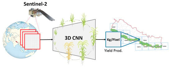
:Crop yield estimation is a major issue of crop monitoring which remains particularly challenging in developing countries due to the problem of timely and adequate data availability. Whereas traditional agricultural systems mainly rely on scarce ground-survey data, freely available multi-temporal and multi-spectral remote sensing images are excellent tools to support these vulnerable systems by accurately monitoring and estimating crop yields before harvest. In this context, we introduce the use of Sentinel-2 (S2) imagery, with a medium spatial, spectral and temporal resolutions, to estimate rice crop yields in Nepal as a case study. Firstly, we build a new large-scale rice crop database (RicePAL) composed by multi-temporal S2 and climate/soil data from the Terai districts of Nepal. Secondly, we propose a novel 3D Convolutional Neural Network (CNN) adapted to these intrinsic data constraints for the accurate rice crop yield estimation. Thirdly, we study the effect of considering different temporal, climate and soil data configurations in terms of the performance achieved by the proposed approach and several state-of-the-art regression and CNN-based yield estimation methods. The extensive experiments conducted in this work demonstrate the suitability of the proposed CNN-based framework for rice crop yield estimation in the developing country of Nepal using S2 data.
1. Introduction
The 2030 Agenda for Sustainable Development of the United Nations [1] has explicitly defined that ending hunger, achieving food security and promoting sustainable agriculture are primary goals for our planet. To this extent, remote sensing imagery [2] plays a fundamental role as a supporting tool for detecting inadequate or poor crop growing conditions, monitoring crops and estimating their corresponding productions [3]. Despite recent technological advances [4,5,6], the increasing population and climate change still raise important challenges for agricultural systems in terms of productivity, security and sustainability [7,8], especially in the context of developing countries [9]. Although there is not an established convention for such designation, developing countries are generally characterized by having underdeveloped industries that typically lead to important economic vulnerabilities based on the instability of agricultural production along other factors [10]. For instance, it is the case in Southern Asia where the reliability and sustainability of agricultural production systems become particularly critical since many countries experience scarce diversification and productivity in this regard [11]. One of the most representative cases is the country of Nepal, where agriculture is the principal economic activity and rice is its most important crop [12]. However, the immediate and dynamic nature of global anthropogenic changes (including rising population and climatic extremes) generate a growing pressure to traditional agriculture which increasingly demands more accurate crop monitoring and yield prediction tools to ensure the stability of food supply [13,14].
In order to support the agricultural systems of Nepal and other analogous developing countries, freely available multi-temporal and multi-spectral remote sensing images have shown to be excellent tools to effectively monitor crops and their growth stages as well as estimating crop yields before harvest [15,16,17]. Many works in the literature exemplify these facts. For instance, Peng et al. develop in [18] a rice yield estimation model based on the Moderate Resolution Imaging Spectroradiometer (MODIS) and its primary production data. In [19], Hong et al. also use MODIS for estimating rice yields but, in this case, combining the Normalized Difference Vegetation Index (NDVI) with meteorological data. Additionally, other authors analyze the use of alternative indexes for the rice yield estimation problem [20]. Despite the initial success achieved by these and other important methods, the coarse spatial resolution of MODIS (i.e., 250 m) generally makes the use of more accurate remote sensing data preferred. It is the case of Siyal et al. who present in [21] a study to estimate Pakistani rice yields from the Landsat Enhanced Thematic Mapper plus (ETM+) instrument, which provides an improved spatial resolution of 30 m. Analogously, Nuarsa et al. conduct in [22] a similar study but focused on the Bali Province of Indonesia. Certainly, Landsat is able to provide important spatial resolution gains with respect to MODIS for rice yield estimation. However, its limited temporal resolution (16 days) is still an important constraint since it logically reduces the temporal availability of such estimates. As a result, other authors opt for jointly considering data from different instruments to relieve these intra-sensor limitations. For example, Setiyono et al. combine in [23] MODIS and synthetic-aperture radar (SAR) data into a crop growth model in order to produce spatially enhanced rice yield estimates. Nonetheless, involving multi-sensor imagery generally leads to important data processing complexities, in terms of temporal gaps, spectral differences, spatial registration, etc., that may logically affects the resulting performance. In this regard, the possibility of using remote sensing data from sensors with better spatial, spectral and temporal nominal resolutions becomes very attractive for the accurate rice yield estimation.
The recent open availability of Sentinel-2 (S2) imagery with higher spatial, spectral and temporal resolutions has unlocked extensive opportunities for agricultural applications that logically include crop mapping and monitoring [24,25,26]. As part of the Copernicus European Earth Observation program, the S2 mission offers global coverage of terrestrial surfaces by means of medium-resolution multi-spectral data [27]. In particular, S2 includes two identical satellites (S2A launched on 23 June 2015 and S2B followed on 7 March 2017) that incorporate the Multi-Spectral Instrument (MSI). The S2 mission offers an innovative wide-swath of 290 km, a spatial resolution ranging from 10 m to 60 m, a spectral resolution with 13 bands in the visible, near infra-red and shortwave infrared of the electromagnetic spectrum and a temporal resolution with 5 days revisit frequency. With these features, S2 imagery has potential to overcome the aforementioned limitations with coarse satellite images and costly data sources in the yield prediction context. Different works in the remote sensing literature exemplify this trend. For instance, He et al. present in [28] a study to demonstrate the potential of S2 biophysical data for the estimation of cotton yields in the southern United States. Analogously, Zhao et al. test in [29] how different vegetation indices derived from S2 can be useful to accurately predict dry-land wheat yields across Northeastern Australia. In [30], the authors develop a model to estimate potato yield using S2 data and several machine learning algorithms in the municipality of Cuellar, Castilla y León (Spain). Additionally, Kayad et al. conduct in [31] a study to investigate the suitability of using S2 vegetation indices together with machine learning techniques to predict corn grain yield variability in Northern Italy. Hunt et al. also propose in [32] combining S2 with environmental data (e.g., soil, meteorological, etc.) to produce accurate wheat crop yield estimates over different regions of the United Kingdom.
Notwithstanding all the conducted research on crop yield prediction, the advantages of S2 data in the context of developing countries still remains as an open-ended question due to the data scarcity problem often suffered by these particularly vulnerable regions. Existing yield estimation methods mostly rely on survey data and other important variables related to crop growth such as weather, precipitation and soil properties [33,34]. Whereas adequate high quality data can be regularly collected in developed countries [35], the situation is rather different in developing countries where such complete and timely updated information is often very difficult to obtain or even not available [36,37,38]. Undoubtedly, there are several international agencies and programs, e.g., Food and Agriculture Organization (FAO) and Famine Early Warning System (FEWS), that manage remote sensing data for crop monitoring and yield estimation from regional to global scales. However, these kinds of systems do not effectively fulfill the regional needs when it comes to national or local scale actions, including the rice crop yield prediction in the country of Nepal [39]. In these circumstances, the free availability of S2 imagery motivates the use of this convenient data to address such challenges by building sustainable solutions for developing countries.
In order to obtain accurate crop yield estimates, not only high-quality remote sensing data but also advanced and intelligent algorithms are essential. To this extent, deep learning models, such as Convolutional Neural Networks (CNNs), have certainly shown a great potential in several important remote sensing applications, including crop yield prediction [35,40,41]. Whereas traditional regression approaches often require feature engineering and field knowledge to extract relevant characteristics from images, deep learning models have the ability to automatically learn features from multiple data representation levels [42]. As a result, the state-of-the-art on crop type classification and yield estimation has shifted from conventional machine learning algorithms to advanced deep learning classifiers and from depending on only spectral features of single images to jointly using spatial-spectral and temporal information for a better accuracy, e.g., [43,44,45].
With all these considerations in mind, the use of deep learning technologies together with the advantages of S2 imagery can play a fundamental role in relieving current limitations of traditional rice crop yield estimation systems, which are mainly based on crop samples, data surveys and field verification reports [46]. Nonetheless, the operational applicability of such technologies over S2 data has not yet been addressed in the context of developing countries rice production, which is precisely the gap that motivates this work. Specifically, this paper introduces the use of S2 data for rice crop yield prediction with the case study in Nepal and provides an operational deep learning-based framework to this end. Firstly, we review different state-of-the-art algorithms for yield estimation based on which the CNN approach is selected as the core technology of our proposed framework due to its excellent performance [42]. Following, we build a new large-scale rice crop database of Nepal (RicePAL) made of multi-temporal S2 products from 2016 to 2018 and ground-truth rice yield data to validate the proposed approach performance. Thereafter, we propose a novel 3D CNN architecture for the accurate estimation of the rice production by taking advantage of multi-temporal S2 images together with supporting climate and soil information. Finally, an extensive experimental comparison, including several state-of-the-art regression and CNN-based crop yield prediction models, is conducted to validate the effectiveness of the proposed framework while analysing the impact of using different temporal and climate/soil data settings. In brief, the main contributions of this paper can be summarized as follows:
- 1.
- The suitability of using S2 imagery to effectively estimate strategic crop yields in developing countries with a case of study in Nepal and its local rice production is investigated.
- 2.
- A new large-scale rice crop database of Nepal (RicePAL) composed by multi-temporal S2 products and ground-truth rice yield information from 2016 to 2018 is built.
- 3.
- A novel operational CNN-based framework adapted to the intrinsic data constraints of developing countries for the accurate rice yield estimation is designed.
- 4.
- The effect of considering different temporal, climate and soil data configurations in terms of the resulting performance achieved by the proposed approach and several state-of-the-art regression and CNN-based yield estimation methods is studied. The codes related to this work will be released for reproducible research inside the remote sensing community (https://github.com/rufernan/RicePAL accessed on 3 April 2021).
The rest of the paper is organized as follows. Section 2 provides a comprehensive review of the existing state-of-the-art methods on crop yield estimation using remote sensing data. Section 3 introduces the study area and also describes in details the dataset created in this work. Section 4 presents the proposed framework while also describing the considered CNN-based architecture. In Section 5, a comprehensive experimental comparison is conducted to discuss the findings of the experimental designs and performance comparisons in Section 6. Finally, Section 7 concludes the work and also provides some interesting remarks at plausible future research lines.
2. Related Work
In the literature, many studies have shown the advantages of using remote sensing data for crop yield estimation by employing statistical methods based on regression models. For instance, in [47], a piece-wise linear regression method with a break-point is employed to predict corn and soybean yields using NDVI, surface temperature, precipitation and soil moisture. The work in [48] used a step-wise regression method for estimating winter wheat yields using MODIS NDVI data. In [49], the crop yield is estimated with the prediction error of about 10% in the United States Midwest by employing Ordinary Least Squares (OLS) regression model using time-series of MODIS products and a climate dataset. In summary, the classical approach for crop yield estimation is mostly based on the multivariate regression analysis using the relationship between crop yields and agro-environmental variables like vegetation indices, climatic variables and soil moisture. With the advances in machine learning, researchers have also applied other models to remote sensing data for crop yield prediction. For example, in [50], the use of Artificial Neural Network (ANN) through a back-propagation algorithm is introduced in forecasting winter wheat crop yield using remote sensing data to overcome the problem that existed in using traditional statistical algorithms (especially regression models) due to nonlinear character of agricultural ecosystems. The study demonstrated a high accuracy of ANN compared to results from a multi-regression linear model. Among the most commonly used machine learning techniques, it is possible to highlight support vector regresion (SVR), Gaussian process regression (GPR) and multi-layer perceptron (MLP) [51]. These techniques have contributed to improve the accuracy of crop yield prediction. However, they often have the disadvantage of requiring feature engineering, which makes other paradigms generally preferred.
One of the first works employing a deep learning approach for crop yield estimation is [52]. Specifically, this study employed a Caffe-based deep learning regression model to estimate corn crop yield at county-level in the United States. The proposed architecture improved the performance of SVR. Additionally, the work presented in [35] employed CNN and long short-term memory (LSTM) algorithms to predict county-level soybean yields in the United States under the assumption of location invariant. To address spatial and temporal dependencies across data points, the authors of the paper proposed the use of linear Gaussian Process (GP) layer on the top of these neural network architectures. The results demonstrated that CNN and LSTM approaches outperformed the other competing techniques, ridge regression, decision trees and a CNN with three hidden layers which were used as baselines. The final crop yield prediction was improved by the addition of linear GP resulting in a 30% reduction of root mean squared error (RMSE) from baselines. The location invariant assumption proposed by [35] discards the spatial information of satellite imagery which can also be crucial information for crop yield estimation. To overcome this limitation, in [40], a CNN approach based on 3D convolutions that consider both spatial and temporal features for yield prediction is introduced. Firstly, the authors replicated the Histogram CNN model of [35] with the same input dataset and set it as baseline for their approach. Considering the computational cost, a channel compression model was applied to reduce the channel dimension from 10 to 3. Thereafter, a 3D convolution was stacked to the model. The proposed CNN architecture outperformed the replicated Histogram CNN and non-deep learning regressors used as baselines [35] with an average RMSE of 355 kg per hectare (kg/ha). Continuing to the same data, [41] proposed a novel CNN-LSTM model for end-of-season and in-season soybean yield prediction. The network consisted of a CNN followed by LSTM where the CNN learns the spatial features and the LSTM is used to learn the temporal features extracted by the CNN. The model achieved reduced RMSE of average 329.53 kg/ha which was better than CNN and LSTM models. Recently, Ref. [53] applied a CNN model to predict crop yield using NDVI and red, green and blue bands acquired from Unmanned Aerial Vehicle (UAV). The result showed the better performance of CNN architecture with RGB (red, green and blue) data. Ref. [54] proposed a novel CNN architecture which used two separate branches to process RGB and multi-spectral images from UAV to predict rice yield in Southern China. The resulting accuracy outperformed the traditional vegetation index-based regression model. The study also highlighted that, unlike the vegetation index-based regression model, the performance of CNN for yield estimation at the maturing stage is much better and more robust.
Based on the related literature [42], CNN and LSTM are mostly used deep learning algorithms to address the problem for crop yield prediction with high accuracy. On the one hand, when these algorithms are used separately, in [35] it was demonstrated that CNN achieved higher accuracy than LSTM. On the other hand, the combined model, CNN-LSTM performed relatively better in [41]. However, the experiments in [41] were conducted using a long-term dataset with a high temporal dimension. The recent availability in years of the Copernicus S2 data limits the use of the LSTM model in this work. Therefore, CNN is chosen as core technology for the rice crop yield estimation framework presented in this work. Exploring the performance of different CNN-based architectures, the CNN-3D model proposed by [40] achieved the highest accuracy to date and, hence, 3D convolutions will serve as basis of the newly presented architecture.
3. Study Area and Dataset
This section introduces in Section 3.1 the study area and the motivation behind it. The second part (Section 3.2) details the RicePAL dataset that has been created for the experimental part of the work.
3.1. Study Area
The study area considered in this work is based on 20 districts of the Terai region of Nepal that comprise a lowland in southern Nepal. Figure 1 shows the region of interest with the considered districts, their corresponding S2 tiles, elevation profiles and spatial scales. The principal economic activity of Nepal is agriculture, which constitutes about one-third of the Gross Domestic Product (GDP) and employs nearly three quarters of the labor force [55]. Of the total basic crop production, paddy production is the highest in the country, sharing 20.75% of the total GDP from agriculture [56]. Even though the Terai region covers just 23.1% of the total area of the country, it comprises 49% of the total agricultural land. The rice production is mainly located in the Terai districts which contributes about 70% of the total rice production of the country. As a result, the domestic food security of Nepal is critically reliant on the sustainability of the cereal production system of this region. However, the growth rate in the agricultural sector of Nepal is too low to meet the growing food demand of the increasing population, indicating that public and private investments in the agricultural research and development sector would increase cereal productivity in Nepal [57]. Moreover, a high degree of spatial and temporal variability, traditional agricultural practices, climate change and its vulnerability have imposed a serious challenge in effective and sustainable agriculture production in Terai [39].
3.2. Dataset
The dataset created in this work (RicePAL) includes 3-year multi-temporal S2 imagery of the Terai region of Nepal together with the corresponding ground-truth rice crop masks and district level rice yield of the study area. In addition, auxiliary climate and soil data are also included in the dataset to support the yield estimation process. Table 1 summarizes the data description and information sources that have been considered to build our rice crop yield estimation dataset. The following sub-sections provide the corresponding details.
3.2.1. Sentinel-2 Data
The key phases of the rice crop cycle, i.e., start of the season (SoS), the peak of season (PoS) and end of the season (EoS), in the Terai region of Nepal correspond to mid-July, mid-September and mid-November respectively [39]. Therefore, the Level-1C (L1C) products during these key periods were downloaded for the years 2016–2018. In case of missing or corrupted images, products within a week before or after the mid-month were downloaded. In total, 14 sentinel tiles (zone 44 and 45) covered the study area as shown in Figure 1. These S2 L1C products can be freely downloaded from ESA’s Scientific Data Hub in Standard Archive Format for Europe (SAFE) files.
As it was previously mentioned, S2 sensors provide a total of 13 spectral bands with a spatial resolution ranging from 10 m to 60 m. Among these spectral bands, the classical RGB and near-infrared (NIR) bands with 10 m spatial resolution are dedicated to land applications. Among six bands at 20 m resolution, four narrow bands in the vegetation red edge spectral domain and two short-wave infrared (SWIR) large bands are used for snow/ice/cloud detection and moisture stress assessment. The remaining bands at 60 m are dedicated to atmospheric correction and cirrus detection. Both satellites have a wide-swath of 290 km and fly in the same orbit phased at 180 providing a relatively high temporal resolution with a revisit frequency of 5 days for S2 operational data products [58]. S2 L1C and Level-2A (L2A) products are provided in tiles which consist of 100 × 100 km ortho-images in UTM/WGS84 projection. On the one hand, L1C products are Top-of-Atmosphere (TOA) radiance images which are radiometrically and geometrically corrected as well as orthorectified using the global Digital Elevation Model (DEM). On the other hand, L2A products provide Bottom-of-Atmosphere (BOA) reflectance images derived from the corresponding L1C products. For this work, L1C products are considered since L2A products are only available from the end of 2018 for regions outside Europe.
A total of 126 S2 L1C products were downloaded and converted to atmospherically corrected L2A products using the Sen2Cor processor which is based on algorithms proposed in the Atmospheric/Topographic Correction for Satellite Imagery (ATCOR) [59]. Sen2Cor is supported by ESA as a third-party plugin for the S2 toolbox (standalone version). It runs in the ESA Sentinel Application Platform (SNAP) or from the command line. Additionally, topographic correction with a 90 m digital elevation database from CGIAR-CSI (http://www.cgiar-csi.org accessed on 3 April 2021) and cirrus corrections were applied [60]. Topographic correction here is purely radiometric and does not change the image geometry. However, the resulting products showed that cirrus correction with Sen2Cor was not effective. Moreover, the products had significant cloud and cloud shadows. In order to deal with these problems, cloud mask data available with L1C products (that specifies the percentage of cloudy pixels and cirrus pixels) was considered during the post processing of L2A products.
Taking into account the total size of the considered products (over 100 GB) and the high computational cost of managing such data volume, we decided to store the final products in 20 m instead of 10 m spatial resolution. Therefore, the resulting L2A products were all resampled to 20 m. Thereafter, a spatial subset was applied to clip the images to the extent of the study area. Among the 13 spectral bands of S2, the three bands with 60 m resolution (B01, B09 and B10) are dedicated to atmospheric correction and cirrus detection. These bands are typically not considered in crop classification tasks [61] hence, they were excluded from the output data. As a result, four bands resampled to 20 m (B02-B04 and B08) and six bands with a nominal spatial resolution of 20 m (B05-B07, B8A, B11 and B12) were concatenated for the considered data processing chain.
NDVI is the most commonly used indicator to monitor vegetation health and classify vegetation extent [62,63]. Moreover, it can be useful to filter clouds as the reflectance values of clouds in visible bands are higher than that in NIR band producing negative NDVI values similar to water and snow [64]. For these reasons, NDVI was also calculated and included into our dataset. Note that bands B04 and B08 bands represent the red and NIR channels respectively and were used to calculate NDVI as follows:
The resulting NDVI product was introduced as an additional band to the final output data in the GeoTIFF file format. Considering the presence of cloud coverage in the images, cloud mask data available with L1C products was also concatenated with the bands. An option is to use these data to filter the input images when training the corresponding rice crop yield prediction models. In this work, we use these additional bands for filtering purposes, not as input data themselves. Regarding the data contamination and temporal availability, we adopt two different strategies that work at product-level and pixel-level. On the one hand, we only download S2 products with a limited cloud coverage. That is, we set a margin of a week before and after each rice crop period (SoS, PoS and EoS) to make sure that the manually selected products contain the least possible clouds. On the other hand, we use both extra bands (cloud masks and NDVI maps) to filter out clouds as well as non-vegetation pixels from annual data volumes.
3.2.2. Auxiliary Data
The agricultural practice in the study area is mostly dependent on natural irrigation due to lack of irrigation facilities which is one of the production constraints of this region. Since climatic variables have a significant impact on rice crop production, it is important to consider this additional information for the yield estimation process as other related works do [65]. Furthermore, the authors in [53] also suggested that in addition to spectral data, soil and climate information can contribute to further improvements to crop yield estimation results. With all these considerations in mind, we include the following additional auxiliary data for the rice yield estimation process:
Climate data: The considered climatic data are listed in Table 2. These data are made available from the Department of Hydrology and Meteorology, Government of Nepal (https://www.dhm.gov.np/ accessed on 3 April 2021). Considering the time period during which the images were downloaded, 15 days average (1 week before and after the chosen representative dates of the rice crop cycle in Terai) of each of these climatic variables was calculated from the available daily data. An spatial interpolation was performed to re-sample these data at the considered S2 spatial resolution (20 m). Note that this interpolation process is required for producing an uniform data volume with S2 imagery and the available climate data. Besides, it is important to remark that the region of interest (Terai districts) has relatively small topographical variations that make weather conditions more uniform than in other parts of the country. As supported by [66,67], we use the ordinary Gaussian process regression method for conducting the spatial interpolation. The experimental space-time semivariogram was calculated for each climate data and for each time period. Leave one out cross-validation method was used to assess the error associated with the model with parameters, producing a Mean Error (ME) and RMSE. The model parameter with least ME and RMSE are used for surface generation of particular climate data. The resulting raster data were then normalized within the range of [0–1] by using the min-max normalization in order to adjust the input data to a common scale for a better convergence of machine learning algorithms. The min-max normalization is done using the following formula,
where x denotes the original value and is the resulting normalized value. After normalization, similar to the ground-truth rice mask, the normalized climate data in raster format were re-projected, re-sampled and clipped to tiles maintaining the spatial extent of tiles.
Soil Data: Soil data of spatial resolution 250 m were downloaded from Krishi Prabidhi Project site (https://krishiprabidhi.net/ accessed on 3 April 2021) which includes six variables namely boron contain, clay contain, organic matter, PH, sand and total nitrogen. The soil data were normalized within the range of [0–1]. Like the previous data, these data were also re-projected and then re-sampled to 20 m.
3.2.3. Ground-Truth Data
Rice crop mask: Considering the major limitation on the availability of a real high-resolution ground-truth map of rice crops in the study area, the rice mapping approach adopted by [39] was utilized as a supporting tool for the annotation of the considered region of interest. In particular, this procedure employs auxiliary MODIS data over the long-term period 2006–2014 to produce robust ground-truth crop annotations based on the rice classification over the whole period. Once this coarse resolution rice map is produced, we re-project it to the UTM/WGS84 projection and re-sample it into 20 m to generate the corresponding ground-truth rice labels at S2 spatial resolution. Then, we filter this resulting map with the land cover mask produced by [68] with the objective of ensuring that our final ground-truth labels do not include non-agricultural areas if any. Finally, we manually revise the obtained annotations to correct possible deviations with respect to the survey data available in [69]. These final rice labels are used as ground-truth crop maps.
Rice crop yield: We set rice yield data published by the Ministry of Agriculture and Livestock Development (https://mold.gov.np/accessed on 3 April 2021), Government of Nepal, as a target of estimation. The yield data was downloaded for the considered years 2016–2018. While most of the studies discussed in Section 2 were conducted using county-level data, we only have the option of using district-level data (larger administrative unit). The scarcity in ground truth yield data is a major challenge in developing countries like Nepal. That is, the available rice production information provided by the government of Nepal is a scalar value for each one of the 20 Terai districts. Consequently, we compute the average yield per rice pixel at each district by uniformly distributing its total production value over the number of rice pixels within the district (logically using the considered S2 pixel spatial resolution, i.e., 20 × 20 m). To feed the yield data as ground-truth values in the dataset, firstly, the yield values in kg/ha are converted to kg/pixel where the area of each pixel is 400 m. Secondly, the rice pixels from the aforementioned rice mask are labeled with these values. The final results are then again summarized to kg/ha.
4. Methodology
This section describes the methods and configurations considered for the rice crop yield estimation task using the RicePAL archive, including an overview of existing CNN-based models and notations (Section 4.1) as well as the details of the proposed architecture (Section 4.2 and Section 4.3).
4.1. Convolutional Neural Networks
CNNs are biologically inspired feed-forward neural networks that extend the classical artificial neural network approach by adding multiple convolutional layers and filters that allow representing the input data in a hierarchical way [70]. In this work, the input data are taken from multi-spectral and multi-temporal S2 images together with auxiliary supporting data which are considered as additional image bands. Let us suppose a multi-spectral image where M, D, H are the spectral bands, width and height, respectively. The pixel of X (with and ) can be defined as the spectral vector . Let us define a neighboring region (image patch) around , composed of pixels from to . With q taking account of the spectral information, it can be redefined as . In this way, a CNN takes a image patch with M channels centered at a pixel and K kernels with a size. Let be the pixel value at the output feature map and be the weight value at position, k-th filter and m band. Let represent the bias of the k-th filter. Depending on the nature of the convolutions, it is possible to distinguish two different types of CNN-based architectures that have been successfully used in crop yield prediction tasks:
- 2D-CNN [53], also called spatial methods, which consider the input data as a complete spatial-spectral volume where the kernel slides along the two spatial dimensions (i.e., width and height). Hence, the multi-temporal data are considered as part of the spectral dimension and the kernel depth is adjusted to the number of available channels. The basic idea consists in treating each channel independently and generating a two-dimensional feature map for each input data volume. More specifically, the convolution process over a multi-spectral input can be defined as follows,
- 3D-CNN [40], also known as spatio-temporal methods, that introduce an additional temporal dimension to allow the convolutional kernel to operate over a specific timestamp window. In a 2D-CNN, all the spatio-temporal data are stacked together in the input and, after the first convolution, the temporal information is completely collapsed [71]. To prevent this, 3D-CNN models make use of 3D convolutions that apply 3-dimensional kernels which slide along width, height and time image dimensions. In this case, each kernel generates a 3D feature map for each spatial-spectral and temporal data volume. Following the aforementioned notation, it is possible to formulate this kind of convolution as,where T is the third dimension of the convolution and represents the number timestamps.
Although it will be fully analyzed in the next section, it is worth mentioning at this point that the proposed architecture will employ the 3D-CNN scheme by implementing 3D convolutional layers. In more details, the proposed architecture will be made of the following types of CNN-based layers:
- 1.
- Convolutional layers (Conv3D): The convolution layer computes the output of neurons that are connected to the local regions in the input image by conducting dot product between their weights and biases at a specific region to which they are related in the input range [72]. Mathematically,where is the output of the l-th convolution layer, is weight matrix defined by the filter bank with kernel size and is the bias of the l-th convolution layer. represents the nonlinear activation function.
- 2.
- Nonlinear layers (Rectified Linear Unit—ReLU): Activation functions are used to embed non-linearity into the neural network thereby enabling the network to learn nonlinear representations. In this layer, the Rectified Linear Unit (ReLU) [73] has been implemented as it is proven to be computationally efficient as well as effective for convergence.
- 3.
- Batch normalization (BN): The batch normalization represents a type of layer aimed at reducing the co-variance shift by normalizing the layer’s inputs over a mini-batch. It enables an independent learning process in each layer and regularizes as well as accelerates the training process. Formally, it can be defined as,where is the expectation operator, and are learnable parameter vectors and is a parameter for numerical stability.
- 4.
- Pooling layers (Pool): The pooling layer is a sub-sampling operation along the dimensions of the feature maps, which does some spatial invariance [72]. Usually, in pooling, some predefined functions (e.g., maximum, average, etc.) are applied to summarize the signal and spatially preserving discriminant information.
- 5.
- Fully connected layers (FC): The fully connected layer takes the output of the previous layers and flattens them into a single vector of values. Then, each output neuron is fully connected to this data vector in order to represent the activation that a certain feature map produces to one of the predefined outputs.
4.2. Proposed Yield Prediction Network
In the context of rice crop yield estimation, considering multi-temporal data may logically provide a better understanding of the seasonal crop growth in order to produce more accurate yield predictions [74]. When it comes to CNNs, it is possible to find the two aforementioned convolutional strategies for exploiting such multi-temporal data [35,40]. On the one hand, 2D-CNN approaches simply stack all the available temporal information into a single input 3D tensor in order to apply the filters over the multi-temporal channels. On the the hand, 3D-CNN models provide a more general scheme since the different temporal observations are embedded into a new spatial dimension that allows the 3D convolutional kernel to have an additional degree of freedom to better detect temporal correlations. In this scenario, the 3D-CNN design allows extracting dynamic features through consecutive time periods, which logically plays a fundamental role in the growing stages of rice crops. Besides, it also allows relieving the long-term temporal limitations of S2 data (available from 2016) while performing a full spatio-spectral and temporal feature extraction for the rice crop yield estimation task. Based on these motivations and also supported by the results achieved in other works [40], the proposed architecture is based on the 3D-CNN approach to effectively exploit spatio-spectral and temporal features from S2 imagery for the accurate rice crop yield prediction in Nepal. Figure 2 shows the building blocks that will constitute the proposed 3D-CNN network. Specifically, we define three different blocks, i.e., head (HB), body (BB) and tail (TB), where K, N, T and U represent the number of kernels, kernel size, number of timestamps and considered fully connected units, respectively. Note that all pooling layers (Pool) are applied over spatial and temporal dimensions using a 3-dimensional stride and the two convolutinal layers of the body block have the same dimensions. Considering these building blocks, Figure 3 displays a graphical visualization of the proposed 3D-CNN architecture for rice crop yield estimation, which is composed of the following constituent parts:
- 1.
- Network’s Head: The proposed architecture starts with two initial head building blocks (HB) that transform the input patches with the multi-temporal data into a first-level feature representation that will be fed to the subsequent network parts. Note that input patches have a size, where M is the total number of bands (made of the concatenation of S2 spectral bands and climate/soil data), P is the spatial size of the input data and T is the temporal dimension representing the considered rice seasons (SoS, PoS and EoS). As it is possible to see, each one of these head blocks is made of four layers: (1) Conv3D, (2) BN, (3) ReLU and (4) Pool. In the case of (1), we employ and convolutional kernels in and , respectively, with a size (). In the case of (4), a max pooling is conducted to reduce the spatial size of the resulting feature maps.
- 2.
- Network’s Body: This part can be considered as the main body of the network since it contains its highest structural complexity. More specifically, the network’s body consists of two sequential building blocks (BB) with the following seven layers: (1) Conv3D, (2) BN, (3) ReLU, (4) Conv3D, (5) BN, (6) ReLU and (7) Pool. This configuration allows us to increase the block depth without reducing the size of the feature maps which eventually produces higher-level features over the same spatio-temporal receptive field. It is important to note that both (1) and (4) layers are defined with the same settings to work towards those high-level features that may help the most to predict the corresponding yield estimations. More specifically, we use and convolutional kernels in and , with a size (). In the case of (7), we conduct a max pooling in to reduce the spatial size while maintaining the depth of the feature maps. Finally, we apply in a max pooling of to summarize the temporal dimension after the network’s body.
- 3.
- Network’s Tail: Once the head and body of the network have been executed, an output 3D volume with deep multi-temporal features is produced. In this way, the last part of the proposed network aims at projecting these high-level feature maps onto their corresponding rice crop yield values. To achieve this goal, we initially define a tail building block (TB) with the following layers: (1) FC, (2) BN and (3) ReLU. Then, we use a final fully connected layer (FC) to generate the desired yield estimates. In the case of (1), we employ fully connected neurons in . In the case of FC, we logically make use of only one neuron to produce a single output for a given multi-temporal input.
4.3. Proposed Network Training
When considering the presented RicePAL dataset, the maximum number of input channels for each timestamp is 20 (10 S2 bands, 4 climate bands and 6 soil bands), where each group of channels is normalized to the [0,1] range using the min-max normalization (Equation (2)) before feeding the network. Regarding the ground-truth data, annual pixel yield values (kg/pixel) are obtained from Nepalese district-level rice production data. In this scenario, the general training process of the proposed architecture is shown in Figure 4. As it is possible to observe, training patches and their corresponding ground-truth rice yield values are used to learn the network parameters via the half-mean-squared-loss. In more details, the last FC layer of the proposed architecture provides the rice yield estimates. Then, the half mean squared error between these predictions and their ground-truth values is used as figure of merit. Mathematically,
where B represents the number of training patches within a mini-batch, is the n-th ground-truth rice yield value and is the corresponding network prediction for the n-th input. This loss is back-propagated to update the network parameters using the Adaptive Moment Estimation (Adam) optimization algorithm [75]. Specifically, this algorithm calculates an exponential moving average of the gradient and the square gradient and the and parameters control the decay rates of these moving averages. Formally,
where is gradient at the i iteration, and are the estimates of the first moment and second moment of the gradient respectively, and and are two hyperparameters. In practice, the default values for and are 0.9 and 0.999. The biased corrected first and second moment estimates are then computed as:
Finally, these biased corrected moment estimates are used to update parameters using the Adam update rule:
5. Experiments
5.1. Experimental Settings
In order to validate the performance of the proposed rice crop yield estimation network, we considered seven different yield prediction methods in the experimental comparison, including traditional regression approaches and CNN-based models: linear regression (LIN) [48], ridge regression (RID) [76], support vector regression (SVR) [77], Gaussian process regression (GPR) [23], CNN-2D [53], CNN-3D [40] and the proposed network. Using all these methods, we considered four different experimental scenarios over the presented RicePAL dataset,
- Experiment 1: In the first experiment, we tested the performance of the considered rice yield estimation methods when using S2 data with all the possible combinations of the rice crop stages (SoS, PoS and EoS). Note that this scheme led to the following seven multi-temporal data alternatives: SoS, PoS, EoS, SoS/PoS, PoS/EoS, SoS/EoS and SoS/PoS/EoS. In each case, the size of the input data volume was , where T is adjusted to the number of available timestamps.
- Experiment 2: In the second experiment, we used the same multi-temporal configuration as the first experiment but added the climate data into the input data volume, resulting in a input size.
- Experiment 3: In this experiment, we adopted the same scheme as the first one but including the soil data in this case ( size).
- Experiment 4: In the last experiment, we also used the same configuration as the first experiment but including all the available S2, climate and soil data ( size).
In all these scenarios, we trained and test all the considered methods using the same data from all the available years (2016–2018). That is, we extracted patches from RicePAL in a way that central pixels and data partitions were always the same regardless the patch sizes and methods. To avoid uninformative data, we only considered patches that did not contain no-data pixels and whose center pixels contained valid yield information. In this regard, an NDVI threshold below 0.1 was applied to filter non-vegetation and cloud pixels from annual data volumes. Then, we used a 3-pixel step over the available rice crop mask to only extract valid patches. Finally, these patches were randomly split into training and test partitions with the of the data. In the case of regression-based crop yield estimation approaches (LIN, RID, SVR and GPR), we used the pixel-wise spectral information as input and the following training settings: robust fitting with the bi-square weight function (LIN), data standardization (SVR and GPR), radial basis function kernel with automatic scale (SVR) and squared exponential kernel (GPR). In the case of CNN-2D, CNN-3D and the proposed network, we tested five different patch sizes . All the CNN-based methods were trained using the Adam optimizer for 100 epochs. The learning rate and mini-batch size were set to 0.001 and 100 respectively. Besides, early stopping was also used to avoid over-fitting. The rest of the training parameters corresponded to the default values of the considered software environment. For each experiment, the corresponding results were quantitatively evaluated based on the RMSE metric, which was calculated in kg/ha as the original ground-truth yield data were available in the same unit. That is, the available district-level rice production information was initially converted to pixel-level for generating the dataset and training/testing the models. Then, the obtained RMSE results were finally translated from kg/pixel to kg/ha using a conversion factor. Besides, the most competitive methods were also assessed through the visual inspection of their corresponding regression plots and output maps.
Regarding the hardware and software environments, it should be mentioned that all the experiments conducted in this work were built on the top of MATLAB 2019a and they were executed on a Ubuntu 16.04 × 64 server with Intel(R) Core(TM) i7-6850K processor with 64 Gb RAM and a NVIDIA GeForce GTX 1080 Ti 11 GB GPU for parallel processing. The related codes will be released for reproducible research inside the remote sensing community (https://github.com/rufernan/RicePAL accessed on 3 April 2021).
5.2. Results
Table 3, Table 4, Table 5 and Table 6 present the quantitative evaluation of the four considered experimental scenarios based on the RMSE metric. Note that these quantitative results are expressed in kg/ha and each experiment includes a different input data source: experiment 1 uses S2 data (S2), experiment 2 employs S2 and climate data (+C), experiment 3 considers S2 data and soil data (+S) and experiment 4 includes all S2, climate and soil data. As it is possible to see, each table is organized with all the possible crop seasonal combinations in rows, whereas the considered crop yield estimation methods are organized in columns. In more details, each table considers a total of seven rice crop seasonal combinations presented in the following row order: S, P, E, S/P, P/E, S/E and S/P/E. It is important to highlight that S, P and E represent including the seasonal data corresponding to SoS, PoS and EoS, respectively. In this way, the first row (S) only uses data from SoS and the seventh row (S/P/E) contemplates all three rice crop stages included in RicePAL. When it comes to the table columns, the results achieved by the considered regression-based methods (i.e., LIN, RID, SVR and GPR) are presented in the first columns whereas the following ones provides the results obtained by CNN-2D, CNN-3D and the proposed network considering five different patch sizes (i.e., 9, 15, 21, 27 and 33). To summarize the global performance of the methods, the last row of each table shows the average quantitative result of each column. Besides, the best RMSE value of each row is highlighted in bold font to indicate the best method. Table 7 also summarizes the best RMSE (kg/ha) result for each experiment/method. In addition to these tables, Figure 5 depicts the qualitative visual results of rice production (kg/pixel) for experiment 4 with S/P/E-S2+C+S over the T45RUK Sentinel-2 tile in 2018. Moreover, Figure 6 displays the regression plots of the considered CNN-based models for experiment 4 with S/P/E multi-temporal data.
6. Discussion
According to the quantitative results reported in Table 3, Table 4, Table 5 and Table 6, there are several important points which deserve to be mentioned regarding to the performance of the considered methods in the rice crop yield estimation task. When considering traditional regression-based techniques, i.e., LIN, RID, SVR and GPR, it is possible to observe that GPR consistently obtains the best result followed by SVR, whereas LIN and RID clearly show a lower performance. Note that all these regression functions have been trained using pixel-wise spectral information and, under this situation, the most powerful algorithms provide the best results due to the inherent complexity of the yield estimation problem [42]. These outcomes are consistent throughout the four considered experimental scenarios, which reveals the better suitability of SVR and GPR for this kind of problem as supported by other works [23,77]. Nonetheless, the performance of these traditional techniques is very limited from a global perspective since our experimental results show that CNN-based models are able to produce substantial performance gains in the rice crop yield estimation task. As it is possible to see, any of the tested CNN-based networks is certainly able to outperform traditional regression methods by a large margin (regardless the considered patch size and experimental setting), which indicates the higher capabilities of the CNN technology to effectively estimate rice crop yields in Nepal with S2 data. On the one hand, the great potential of CNNs to extract highly discriminating features from a neighboring region (patch) allows generating more accurate yield predictions for a given pixel. On the other hand, the higher resolution of S2 (with respect to other traditional sensors, e.g., MODIS) can even make these convolutional features more informative to map ground-truth yield values in the context of this work.
When analyzing the global results of the considered CNN-based schemes (i.e., CNN-2D, CNN-3D and the proposed network), the proposed network achieves a remarkable improvement with respect to the regression baselines as well as CNN-2D and CNN-3D models. On average, CNN-2D and CNN-3D obtain a global RMSE of and kg/ha, whereas the average result of the proposed model is kg/ha. Even though the three considered CNN models are able to produce substantial gains with respect to the baseline regression methods, the proposed network exhibits the best overall performance, obtaining an average RMSE improvement of and units over CNN-2D and CNN-3D, respectively. By analyzing these results in more details, we will be able to provide a better understanding of the performance differences among the considered methods and experimental scenarios. In general, the experiments show that using a larger patch size generally provides better results, especially with CNN-3D and the proposed network. Intuitively, we can think that including a larger pixel neighbourhood may provide more information that can be effectively exploited by CNN models. However, the bigger the patch the more complex the data and the more likely to be affected by cloud coverage and other anomalies. Note that, as we increase the patch size, the extracted patches are more likely to be invalid and this fact prevents us to consider patches beyond a certain spatial limit.
In this work, we test five different patch sizes () and the best average results are always achieved with 27 and 33. To this extent, we can observe noteworthy performance differences among the tested CNN-based models. When fixing the patch size to small values (e.g., ), it is possible to see that CNN-2D obtains better results than CNN-3D, whereas considering larger patch sizes (e.g., ) makes CNN-3D work better. This observation can be explained from the perspective of the data and model complexities. As it was previously mentioned, the larger the patch size the higher the data complexity and, hence, intricate models are expected to better exploit such data. In this sense, the additional temporal dimension of CNN-3D increases the number of network parameters, which eventually makes this method take better advantage of larger patches. In contrast, the proposed network has been designed to control the total number of layers (likewise in CNN-2D) while defining 3D convolutional blocks that work for reducing over-fitting, which allows us to provide competitive advantages with respect to CNN-2D and CNN-3D models regardless the patch size.
In relation to the considered experimental settings, it is important to analyze how the different data sources and temporal timestamps affect the rice yield estimation task. In all the conducted experiments, we can observe that, in general, the joint use of SoS, PoS and EoS temporal information (i.e., S/P/E) consistently provides better results than using any other data combination. Despite the fact that it is possible to find few exceptions, this trend makes sense from an intuitive perspective since the better we model the rice crop cycle via the input images, the corresponding yield predictions are logically expected to be better. In the case of analyzing the effect of the different data sources (i.e., S2, +C and +S), we can also make important observations. To facilitate this analysis, Table 1 presents a summary with the best RMSE (kg/ha) results for each experiment and method. As one can see, all the regression algorithms are able to obtain the best results when using S2 imagery together with climate and soil data (experiment 4). Precisely, this outcome indicates that the limitations of these traditional methods to uncover features from the pixel spatial neighbourhood make the use of supporting climate and soil data highly suitable. Nonetheless, the situation is rather different with CNN-based models. More specifically, it is possible to observe two general trends depending on the considered patch size. On the one hand, the use of climate and soil data (experiment 4) with small patches (e.g., ) tends to provide certain performance gains in the rice crop yield estimation task. For instance, CNN-2D with produces the minimum RMSE value in experiment 4, whereas CNN-3D and the proposed network do the same with . On the other hand, the use of larger patches (e.g., ) shows that S2 imagery (experiment 1) generally becomes more effective than other data source combinations. In the context of this work, this fact reveals that CNN-based methods do not necessarily require additional supporting data when using large input patches since they are able to uncover useful features from the pixel neighborhood. As it is possible to see in Table 1, CNN-2D, CNN-3D and the proposed network obtain the best RMSE result in experiment 1 when considering . Another important remark can be made when comparing the inclusion of climate (experiment 2) and soil data (experiment 3). According to the reported results, climate information seems to work slightly better than soil with traditionally regression algorithms, whereas CNN models show the opposite trend. Once again, these differences can be caused by the aforementioned data complexity since the number of soil bands (6) is higher than climate bands (4) and, hence, it may benefit all CNN models and particularly the proposed approach.
All in all, the newly defined network consistently shows the best performances over all the tested scenarios which indicate its higher suitability for estimating rice crop yields in Nepal from S2 data. The main advantage of the proposed architecture, over CNN-2D and CNN-3D, lies on its ability to effectively balance two aspects that play a key role in the crop yield estimation task: multi-temporal information and contextual limitations. Firstly, the presented approach takes advantage of 3D convolutions to introduce an additional temporal dimension to allow generating multi-temporal features which do not necessarily depends on the spectral information itself. That is, seasonal data can be better differentiated from the spectral ones and hence better exploited for the annual rice crop yield prediction. Secondly, the proposed network also accounts for the data limitations that may occur, especially in the context of developing countries. In other words, the use of 3D convolutions logically increases the model complexity and, in this scenario, the over-fitting problem may become an important issue with limited data. Note that it is possible see this effect when comparing the performances of CNN-2D and CNN-3D with small patch sizes, e.g., Table 3. To relieve this problem, we propose a new architecture which make use of two different 3D convolutional building blocks that work for reducing the network over-fitting. In contrast to CNN-3D, the proposed approach reduces the total number of convolutional layers. Besides, it avoids the need of using an initial compression module while defining new blocks to make the training process more effective regardless the input patch size and auxiliary data availability. These results are supported by the qualitative regression maps displayed in Figure 5. According to the corresponding image details, the proposed approach provides the visual result most similar to the ground-truth rice yield map since it is able to relieve an important part of the output noise generated by the other yield prediction methods. Figure 6 displays the regression plots corresponding to the results of experiment 4 with S/P/E-S2+C+S. As it is possible to see, CNN-3D is able to provide better results than CNN-2D, especially when increasing the patch size. Nonetheless, the regression adjustment provided by the proposed network is certainly the most accurate which supports its better performance for the problem of estimating rice crop yields in Nepal from S2 imagery.
7. Conclusions and Future Work
This work investigated the applicability of multi-temporal S2 and climate/soil data for effectively conducting rice crop yield estimation in developing countries. To achieve this goal, we used the Terai districts of Nepal as a case of study and defined a new large-scale multi-temporal database made of multiple S2 products and ground-truth rice monitoring information. Thereafter, we proposed a novel CNN model adapted to the local data constraints for the accurate rice yield estimation. The experimental part of the work validated the suitability of S2 imagery and the proposed approach, with respect to different state-of-the-art regression-based and deep learning-based crop yield estimation techniques available in the literature.
According to the results of this work, it is possible to draw several important conclusions related to the general use of S2 and auxiliary data. First, the multi-temporal component of S2 imagery is a key factor to improve the rice crop classification accuracy as opposed to the use of single time period images. Second, auxiliary climate and soil data only support the yield estimation process when considering small patch sizes. Third, the proposed yield estimation network is able to provide competitive advantages by jointly exploiting 3D convolutions while reducing over-fitting with limited data. With all this considerations in mind, the presented CNN-based framework proves the feasibility of using multi-temporal S2 images together with the data available in developing countries to automatically conduct rice crop monitoring for contributing in more efficient agriculture systems and practices in coming days. In the future, increasing per year temporal depth of S2 images can be advantageous in the yield estimation process. However, we have to keep in mind that this will also increase the data volume and computational costs, especially when the study area is large like in our case. Considering the limited data availability for the yield estimation process, in the future, the use of pre-trained networks could be explored. Additionally, extending this work to other crop types could also be very interesting.
Author Contributions
The authors have contributed as equally to this work. All authors have read and agreed to the published version of the manuscript.
Funding
This work was supported by the Ministry of Science, Innovation and Universities of Spain (RTI2018-098651-B-C54) and the Valencian Government (GV/2020/167).
Institutional Review Board Statement
Not applicable.
Informed Consent Statement
Not applicable.
Data Availability Statement
The codes related to this work will be released for reproducible research at https://github.com/rufernan/RicePAL (accessed on 3 April 2021).
Conflicts of Interest
The authors declare no conflict of interest.
References
- United Nations. Transforming Our World: The 2030 Agenda for Sustainable Development; United Nations, Department of Economic and Social Affairs: New York, NY, USA, 2015. [Google Scholar]
- Toth, C.; Jóźków, G. Remote sensing platforms and sensors: A survey. ISPRS J. Photogramm. Remote Sens. 2016, 115, 22–36. [Google Scholar] [CrossRef]
- Weiss, M.; Jacob, F.; Duveiller, G. Remote sensing for agricultural applications: A meta-review. Remote Sens. Environ. 2020, 236, 111402. [Google Scholar] [CrossRef]
- Sishodia, R.P.; Ray, R.L.; Singh, S.K. Applications of Remote Sensing in Precision Agriculture: A Review. Remote Sens. 2020, 12, 3136. [Google Scholar] [CrossRef]
- Lu, B.; Dao, P.D.; Liu, J.; He, Y.; Shang, J. Recent Advances of Hyperspectral Imaging Technology and Applications in Agriculture. Remote Sens. 2020, 12, 2659. [Google Scholar] [CrossRef]
- Fernandez-Beltran, R.; Latorre-Carmona, P.; Pla, F. Single-frame super-resolution in remote sensing: A practical overview. Int. J. Remote Sens. 2017, 38, 314–354. [Google Scholar] [CrossRef]
- Kogan, F. Remote Sensing for Food Security; Springer: Berlin/Heidelberg, Germany, 2019. [Google Scholar]
- Kerényi, A.; McIntosh, R.W. Sustainable Development in Changing Complex Earth Systems; Springer: Berlin/Heidelberg, Germany, 2020. [Google Scholar]
- Tey, Y.S.; Li, E.; Bruwer, J.; Abdullah, A.M.; Brindal, M.; Radam, A.; Ismail, M.M.; Darham, S. Factors influencing the adoption of sustainable agricultural practices in developing countries: A review. Environ. Eng. Manag. J. 2017, 16, 337–349. [Google Scholar] [CrossRef]
- Haraguchi, N.; Martorano, B.; Sanfilippo, M. What factors drive successful industrialization? Evidence and implications for developing countries. Struct. Chang. Econ. Dyn. 2019, 49, 266–276. [Google Scholar] [CrossRef]
- Roy, T. The Economy of South Asia: From 1950 to the Present; Springer: Berlin/Heidelberg, Germany, 2017. [Google Scholar]
- Gadal, N.; Shrestha, J.; Poudel, M.N.; Pokharel, B. A review on production status and growing environments of rice in Nepal and in the world. Arch. Agric. Environ. Sci. 2019, 4, 83–87. [Google Scholar] [CrossRef]
- Chalise, S.; Naranpanawa, A. Climate change adaptation in agriculture: A computable general equilibrium analysis of land-use change in Nepal. Land Use Policy 2016, 59, 241–250. [Google Scholar] [CrossRef] [Green Version]
- Paudel, M.N. Prospects and limitations of agriculture industrialization in Nepal. Agron. J. Nepal 2016, 4, 38–63. [Google Scholar] [CrossRef] [Green Version]
- Chauhan, S.; Darvishzadeh, R.; Boschetti, M.; Pepe, M.; Nelson, A. Remote sensing-based crop lodging assessment: Current status and perspectives. ISPRS J. Photogramm. Remote Sens. 2019, 151, 124–140. [Google Scholar] [CrossRef] [Green Version]
- Wang, L.; Zhang, G.; Wang, Z.; Liu, J.; Shang, J.; Liang, L. Bibliometric Analysis of Remote Sensing Research Trend in Crop Growth Monitoring: A Case Study in China. Remote Sens. 2019, 11, 809. [Google Scholar] [CrossRef] [Green Version]
- Awad, M.M. Toward precision in crop yield estimation using remote sensing and optimization techniques. Agriculture 2019, 9, 54. [Google Scholar] [CrossRef] [Green Version]
- Peng, D.; Huang, J.; Li, C.; Liu, L.; Huang, W.; Wang, F.; Yang, X. Modelling paddy rice yield using MODIS data. Agric. For. Meteorol. 2014, 184, 107–116. [Google Scholar] [CrossRef]
- Hong, S.Y.; Hur, J.; Ahn, J.B.; Lee, J.M.; Min, B.K.; Lee, C.K.; Kim, Y.; Lee, K.D.; Kim, S.H.; Kim, G.Y.; et al. Estimating rice yield using MODIS NDVI and meteorological data in Korea. Korean J. Remote Sens. 2012, 28, 509–520. [Google Scholar] [CrossRef]
- Son, N.; Chen, C.; Chen, C.; Minh, V.; Trung, N. A comparative analysis of multitemporal MODIS EVI and NDVI data for large-scale rice yield estimation. Agric. For. Meteorol. 2014, 197, 52–64. [Google Scholar] [CrossRef]
- Siyal, A.A.; Dempewolf, J.; Becker-Reshef, I. Rice yield estimation using Landsat ETM+ Data. J. Appl. Remote Sens. 2015, 9, 095986. [Google Scholar] [CrossRef]
- Nuarsa, I.W.; Nishio, F.; Hongo, C. Rice yield estimation using Landsat ETM+ data and field observation. J. Agric. Sci. 2012, 4, 45. [Google Scholar] [CrossRef] [Green Version]
- Setiyono, T.D.; Quicho, E.D.; Gatti, L.; Campos-Taberner, M.; Busetto, L.; Collivignarelli, F.; García-Haro, F.J.; Boschetti, M.; Khan, N.I.; Holecz, F. Spatial rice yield estimation based on MODIS and Sentinel-1 SAR data and ORYZA crop growth model. Remote Sens. 2018, 10, 293. [Google Scholar] [CrossRef] [Green Version]
- You, N.; Dong, J. Examining earliest identifiable timing of crops using all available Sentinel 1/2 imagery and Google Earth Engine. ISPRS J. Photogramm. Remote Sens. 2020, 161, 109–123. [Google Scholar] [CrossRef]
- Ashourloo, D.; Shahrabi, H.S.; Azadbakht, M.; Aghighi, H.; Nematollahi, H.; Alimohammadi, A.; Matkan, A.A. Automatic canola mapping using time series of sentinel 2 images. ISPRS J. Photogramm. Remote Sens. 2019, 156, 63–76. [Google Scholar] [CrossRef]
- Mercier, A.; Betbeder, J.; Baudry, J.; Le Roux, V.; Spicher, F.; Lacoux, J.; Roger, D.; Hubert-Moy, L. Evaluation of Sentinel-1 & 2 time series for predicting wheat and rapeseed phenological stages. ISPRS J. Photogramm. Remote Sens. 2020, 163, 231–256. [Google Scholar]
- Drusch, M.; Del Bello, U.; Carlier, S.; Colin, O.; Fernandez, V.; Gascon, F.; Hoersch, B.; Isola, C.; Laberinti, P.; Martimort, P.; et al. Sentinel-2: ESA’s optical high-resolution mission for GMES operational services. Remote Sens. Environ. 2012, 120, 25–36. [Google Scholar] [CrossRef]
- He, L.; Mostovoy, G. Cotton Yield Estimate Using Sentinel-2 Data and an Ecosystem Model over the Southern US. Remote Sens. 2019, 11, 2000. [Google Scholar] [CrossRef] [Green Version]
- Zhao, Y.; Potgieter, A.B.; Zhang, M.; Wu, B.; Hammer, G.L. Predicting wheat yield at the field scale by combining high-resolution Sentinel-2 satellite imagery and crop modelling. Remote Sens. 2020, 12, 1024. [Google Scholar] [CrossRef] [Green Version]
- Gómez, D.; Salvador, P.; Sanz, J.; Casanova, J.L. Potato yield prediction using machine learning techniques and sentinel 2 data. Remote Sens. 2019, 11, 1745. [Google Scholar] [CrossRef] [Green Version]
- Kayad, A.; Sozzi, M.; Gatto, S.; Marinello, F.; Pirotti, F. Monitoring Within-Field Variability of Corn Yield using Sentinel-2 and Machine Learning Techniques. Remote Sens. 2019, 11, 2873. [Google Scholar] [CrossRef] [Green Version]
- Hunt, M.L.; Blackburn, G.A.; Carrasco, L.; Redhead, J.W.; Rowland, C.S. High resolution wheat yield mapping using Sentinel-2. Remote Sens. Environ. 2019, 233, 111410. [Google Scholar] [CrossRef]
- De Wit, A.; Clevers, J. Efficiency and accuracy of per-field classification for operational crop mapping. Int. J. Remote Sens. 2004, 25, 4091–4112. [Google Scholar] [CrossRef]
- Waldner, F.; Canto, G.S.; Defourny, P. Automated annual cropland mapping using knowledge-based temporal features. ISPRS J. Photogramm. Remote Sens. 2015, 110, 1–13. [Google Scholar] [CrossRef]
- You, J.; Li, X.; Low, M.; Lobell, D.; Ermon, S. Deep gaussian process for crop yield prediction based on remote sensing data. In Proceedings of the Thirty-First AAAI Conference on Artificial Intelligence, San Francisco, CA, USA, 4–9 February 2017; pp. 4559–4565. [Google Scholar]
- Gumma, M.K.; Thenkabail, P.S.; Maunahan, A.; Islam, S.; Nelson, A. Mapping seasonal rice cropland extent and area in the high cropping intensity environment of Bangladesh using MODIS 500 m data for the year 2010. ISPRS J. Photogramm. Remote Sens. 2014, 91, 98–113. [Google Scholar] [CrossRef]
- Picoli, M.C.A.; Camara, G.; Sanches, I.; Simões, R.; Carvalho, A.; Maciel, A.; Coutinho, A.; Esquerdo, J.; Antunes, J.; Begotti, R.A.; et al. Big earth observation time series analysis for monitoring Brazilian agriculture. ISPRS J. Photogramm. Remote Sens. 2018, 145, 328–339. [Google Scholar] [CrossRef]
- Song, P.; Mansaray, L.R.; Huang, J.; Huang, W. Mapping paddy rice agriculture over China using AMSR-E time series data. ISPRS J. Photogramm. Remote Sens. 2018, 144, 469–482. [Google Scholar] [CrossRef]
- Qamer, F.M.; Shah, S.P.; Murthy, M.; Baidar, T.; Dhonju, K.; Hari, B.G. Operationalizing crop monitoring system for informed decision making related to food security in Nepal. Int. Arch. Photogramm. Remote Sens. Spat. Inf. Sci. 2014, 40, 1325. [Google Scholar] [CrossRef] [Green Version]
- Russello, H. Convolutional Neural Networks for Crop Yield Prediction Using Satellite Images; IBM Center for Advanced Studies, University of Amsterdam: Amsterdam, The Netherlands, 2018. [Google Scholar]
- Sun, J.; Di, L.; Sun, Z.; Shen, Y.; Lai, Z. County-Level Soybean Yield Prediction Using Deep CNN-LSTM Model. Sensors 2019, 19, 4363. [Google Scholar] [CrossRef] [Green Version]
- Van Klompenburg, T.; Kassahun, A.; Catal, C. Crop yield prediction using machine learning: A systematic literature review. Comput. Electron. Agric. 2020, 177, 105709. [Google Scholar] [CrossRef]
- Kussul, N.; Lavreniuk, M.; Skakun, S.; Shelestov, A. Deep learning classification of land cover and crop types using remote sensing data. IEEE Geosci. Remote Sens. Lett. 2017, 14, 778–782. [Google Scholar] [CrossRef]
- Cai, Y.; Guan, K.; Peng, J.; Wang, S.; Seifert, C.; Wardlow, B.; Li, Z. A high-performance and in-season classification system of field-level crop types using time-series Landsat data and a machine learning approach. Remote Sens. Environ. 2018, 210, 35–47. [Google Scholar] [CrossRef]
- Dyson, J.; Mancini, A.; Frontoni, E.; Zingaretti, P. Deep learning for soil and crop segmentation from remotely sensed data. Remote Sens. 2019, 11, 1859. [Google Scholar] [CrossRef] [Green Version]
- Shrisath, P. Real-Time Crop Yield Monitoring in Nepal for Food Security Planning and Climatic Risk Management; CGIAR Research Program on Climate Change Agriculture and Food Security, International Water Management Institute (IWMI): Kathmandu, Nepal, 2016. [Google Scholar]
- Prasad, A.K.; Chai, L.; Singh, R.P.; Kafatos, M. Crop yield estimation model for Iowa using remote sensing and surface parameters. Int. J. Appl. Earth Obs. Geoinf. 2006, 8, 26–33. [Google Scholar] [CrossRef]
- Ren, J.; Chen, Z.; Zhou, Q.; Tang, H. Regional yield estimation for winter wheat with MODIS-NDVI data in Shandong, China. Int. J. Appl. Earth Obs. Geoinf. 2008, 10, 403–413. [Google Scholar] [CrossRef]
- Kim, N.; Lee, Y.W. Estimation of corn and soybeans yield using remote sensing and crop yield data in the United States. In Remote Sensing for Agriculture, Ecosystems, and Hydrology XVI; International Society for Optics and Photonics: Washington, DC, USA, 2014; Volume 9239. [Google Scholar]
- Jiang, D.; Yang, X.; Clinton, N.; Wang, N. An artificial neural network model for estimating crop yields using remotely sensed information. Int. J. Remote Sens. 2004, 25, 1723–1732. [Google Scholar] [CrossRef]
- Kim, N.; Lee, Y.W. Machine learning approaches to corn yield estimation using satellite images and climate data: A case of Iowa State. J. Korean Soc. Surv. Geod. Photogramm. Cartogr. 2016, 34, 383–390. [Google Scholar] [CrossRef]
- Kuwata, K.; Shibasaki, R. Estimating crop yields with deep learning and remotely sensed data. In Proceedings of the 2015 IEEE International Geoscience and Remote Sensing Symposium (IGARSS), Milan, Italy, 26–31 July 2015; pp. 858–861. [Google Scholar]
- Nevavuori, P.; Narra, N.; Lipping, T. Crop yield prediction with deep convolutional neural networks. Comput. Electron. Agric. 2019, 163, 104859. [Google Scholar] [CrossRef]
- Yang, Q.; Shi, L.; Han, J.; Zha, Y.; Zhu, P. Deep convolutional neural networks for rice grain yield estimation at the ripening stage using UAV-based remotely sensed images. Field Crop. Res. 2019, 235, 142–153. [Google Scholar] [CrossRef]
- MOF. Economic Survey, Fiscal Year 2009/10; Technical Report; Ministry of Finance (MOF), Government of Nepal: Kathmandu, Nepal, 2010.
- MOAC. Statistical Information on Nepalese Agriculture, 2008/2009; Technical Report; Agri-Business Promotion and Statistical Division, Ministry of Agriculture and Cooperatives: Kathmandu, Nepal, 2009.
- Ghimire, S.; Dhungana, S.M.; Krishna, V.; Teufel, N.; Sherchan, D. Biophysical and Socio-Economic Characterization of Cereal Production Systems of Central Nepal; CIMMYT Research Data & Software Repository Network: Mexico City, Mexico, 2013. [Google Scholar]
- Gascon, F.; Cadau, E.; Colin, O.; Hoersch, B.; Isola, C.; Fernández, B.L.; Martimort, P. Copernicus Sentinel-2 mission: Products, algorithms and Cal/Val. In Earth Observing Systems XIX; International Society for Optics and Photonics: Washington, DC, USA, 2014; Volume 9218, p. 92181E. [Google Scholar]
- Richter, R.; Schläpfer, D. Atmospheric/Topographic Correction for Satellite Imagery (ATCOR-2/3 User Guide, Version 8.3. 1, February 2014). ReSe Appl. Schläpfer Langeggweg 2013, 3, 77. [Google Scholar]
- Vuolo, F.; Żółtak, M.; Pipitone, C.; Zappa, L.; Wenng, H.; Immitzer, M.; Weiss, M.; Baret, F.; Atzberger, C. Data service platform for Sentinel-2 surface reflectance and value-added products: System use and examples. Remote Sens. 2016, 8, 938. [Google Scholar] [CrossRef] [Green Version]
- Immitzer, M.; Vuolo, F.; Atzberger, C. First experience with Sentinel-2 data for crop and tree species classifications in central Europe. Remote Sens. 2016, 8, 166. [Google Scholar] [CrossRef]
- Fan, X.; Liu, Y. A global study of NDVI difference among moderate-resolution satellite sensors. ISPRS J. Photogramm. Remote Sens. 2016, 121, 177–191. [Google Scholar] [CrossRef]
- De la Casa, A.; Ovando, G.; Bressanini, L.; Martinez, J.; Diaz, G.; Miranda, C. Soybean crop coverage estimation from NDVI images with different spatial resolution to evaluate yield variability in a plot. ISPRS J. Photogramm. Remote Sens. 2018, 146, 531–547. [Google Scholar] [CrossRef]
- Bai, T.; Li, D.; Sun, K.; Chen, Y.; Li, W. Cloud detection for high-resolution satellite imagery using machine learning and multi-feature fusion. Remote Sens. 2016, 8, 715. [Google Scholar] [CrossRef] [Green Version]
- Gandhi, N.; Armstrong, L.J.; Petkar, O.; Tripathy, A.K. Rice crop yield prediction in India using support vector machines. In Proceedings of the 2016 13th International Joint Conference on Computer Science and Software Engineering (JCSSE), Khon Kaen, Thailand, 13–15 July 2016; pp. 1–5. [Google Scholar]
- Karki, R.; Talchabhadel, R.; Aalto, J.; Baidya, S.K. New climatic classification of Nepal. Theor. Appl. Climatol. 2016, 125, 799–808. [Google Scholar] [CrossRef]
- Shrestha, S.; Baidar, T. Spatial Distribution and Temporal Change of Extreme Precipitation Events on the Koshi Basin of Nepal. Nepal. J. Geoinform. 2018, 17, 38–46. [Google Scholar]
- Uddin, K.; Shrestha, H.L.; Murthy, M.; Bajracharya, B.; Shrestha, B.; Gilani, H.; Pradhan, S.; Dangol, B. Development of 2010 national land cover database for the Nepal. J. Environ. Manag. 2015, 148, 82–90. [Google Scholar] [CrossRef]
- Paudel, G.; Maharjan, S.; Guerena, D.; Rai, A.; McDonald, A.J. Nepal Rice Crop Cut and Survey Data 2016; CIMMYT Research Data & Software Repository Network: Mexico City, Mexico, 2017. [Google Scholar]
- Schmidhuber, J. Deep learning in neural networks: An overview. Neural Netw. 2015, 61, 85–117. [Google Scholar] [CrossRef] [Green Version]
- Ji, S.; Zhang, C.; Xu, A.; Shi, Y.; Duan, Y. 3D convolutional neural networks for crop classification with multi-temporal remote sensing images. Remote Sens. 2018, 10, 75. [Google Scholar] [CrossRef] [Green Version]
- O’Shea, K.; Nash, R. An introduction to convolutional neural networks. arXiv 2015, arXiv:1511.08458. [Google Scholar]
- Dahl, G.E.; Sainath, T.N.; Hinton, G.E. Improving deep neural networks for LVCSR using rectified linear units and dropout. In Proceedings of the 2013 IEEE International Conference on Acoustics, Speech and Signal Processing, Vancouver, BC, Canada, 26–31 May 2013; pp. 8609–8613. [Google Scholar]
- Onojeghuo, A.O.; Blackburn, G.A.; Wang, Q.; Atkinson, P.M.; Kindred, D.; Miao, Y. Mapping paddy rice fields by applying machine learning algorithms to multi-temporal Sentinel-1A and Landsat data. Int. J. Remote Sens. 2018, 39, 1042–1067. [Google Scholar] [CrossRef] [Green Version]
- Kingma, D.P.; Ba, J. Adam: A method for stochastic optimization. arXiv 2014, arXiv:1412.6980. [Google Scholar]
- Hernandez, J.; Lobos, G.A.; Matus, I.; Del Pozo, A.; Silva, P.; Galleguillos, M. Using ridge regression models to estimate grain yield from field spectral data in bread wheat (Triticum aestivum L.) grown under three water regimes. Remote Sens. 2015, 7, 2109. [Google Scholar] [CrossRef] [Green Version]
- Shiu, Y.S.; Chuang, Y.C. Yield Estimation of Paddy Rice Based on Satellite Imagery: Comparison of Global and Local Regression Models. Remote Sens. 2019, 11, 111. [Google Scholar] [CrossRef] [Green Version]
Figure 1.
Study area with S2 tiles and elevation profile.

Figure 2.
Building blocks considered for the head (a), body (b) and tail (c) of the proposed architecture. In (a,b), K, N, T and U represent the considered number of kernels, kernel size, number of timestamps and number of fully connected neurons, respectively. Note that, in (b), both 3D convolutinal layers are defined with the same dimensions. Besides, a 3-dimensional stride is used in the pooling layers (Pool) to summarize spatial and temporal dimensions, where appropriate.

Figure 3.
Graphical visualization of the proposed 3D-Convolutional Neural Network (CNN) architecture for rice crop yield estimation. The input rice crop multi-temporal data (start of the season—SoS, peak of season—PoS and end of the season—EoS), made of soil, climate and Sentinel-2 information, are passed through four different 3D convolutional blocks that compose the head and body of the proposed network. Finally, a fully connected block and a final fully connected layer are used to estimate the rice production. Note that M, P and T represent the total number of input channels, patch size and considered timestamps, respectively.

Figure 4.
Training process of the proposed rice yield estimation network.

Figure 5.
Qualitative results (kg/pixel) for experiment 4 with S/P/E-S2+C+S over the T45RUK Sentinel-2 tile in 2018. In the case of CNN-2D, CNN-2D and the proposed network, a 33 patch size is considered.
Figure 5.
Qualitative results (kg/pixel) for experiment 4 with S/P/E-S2+C+S over the T45RUK Sentinel-2 tile in 2018. In the case of CNN-2D, CNN-2D and the proposed network, a 33 patch size is considered.


Figure 6.
Regression plots for experiment 4 with S/P/E-S2+C+S. In rows, the tested patch sizes (9, 15, 21, 27 and 33). In columns, the considered CNN-based methods (CNN-2D, CNN-2D and the proposed network).
Figure 6.
Regression plots for experiment 4 with S/P/E-S2+C+S. In rows, the tested patch sizes (9, 15, 21, 27 and 33). In columns, the considered CNN-based methods (CNN-2D, CNN-2D and the proposed network).


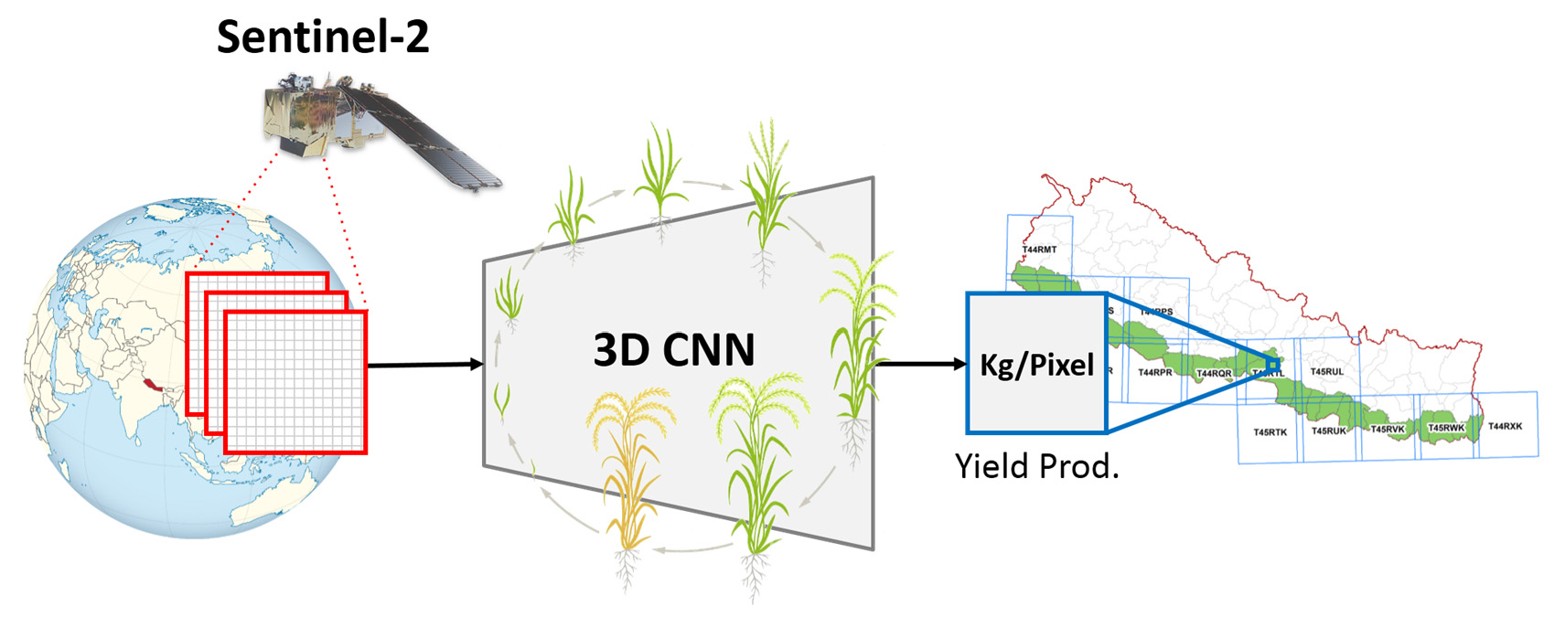
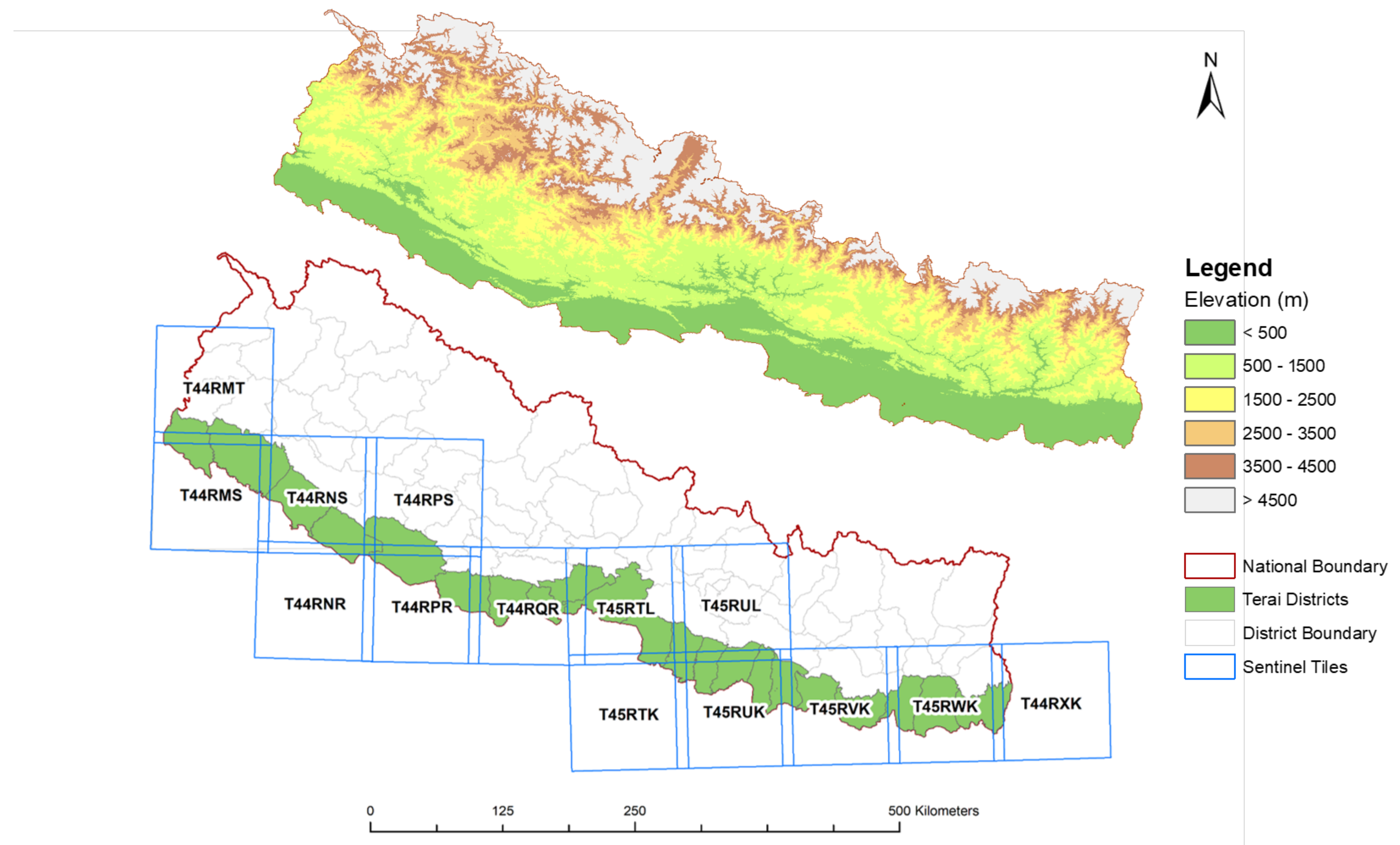
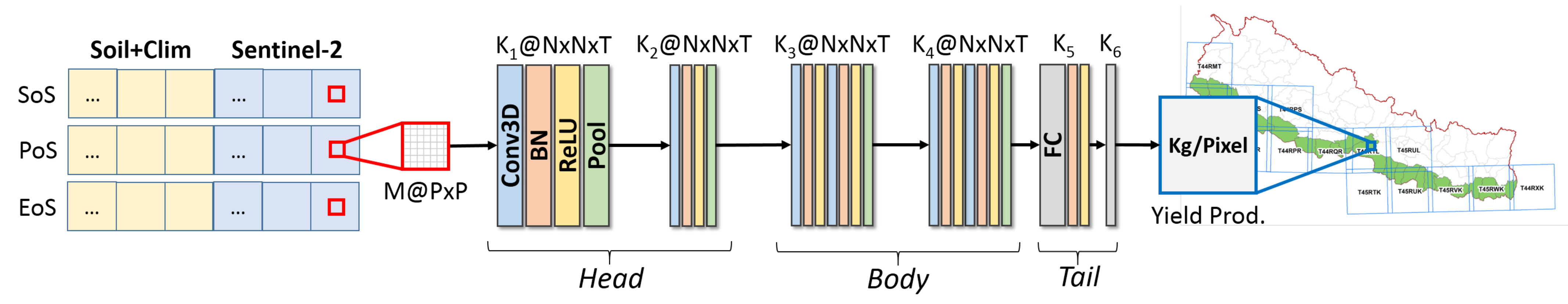
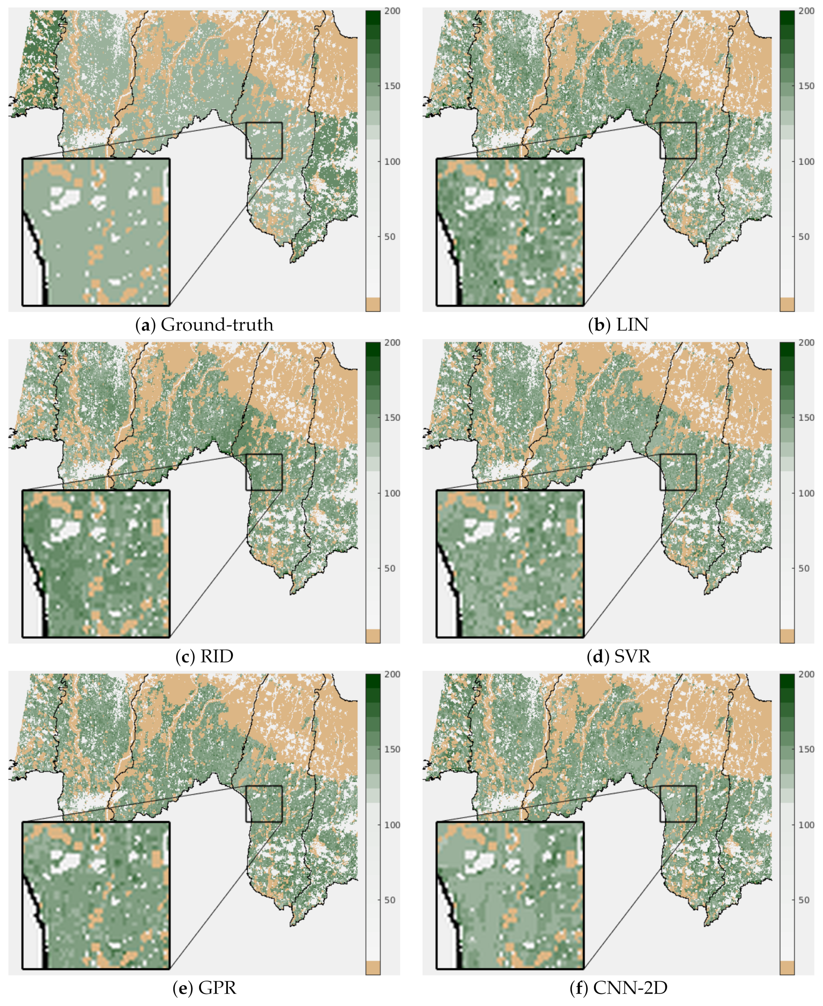
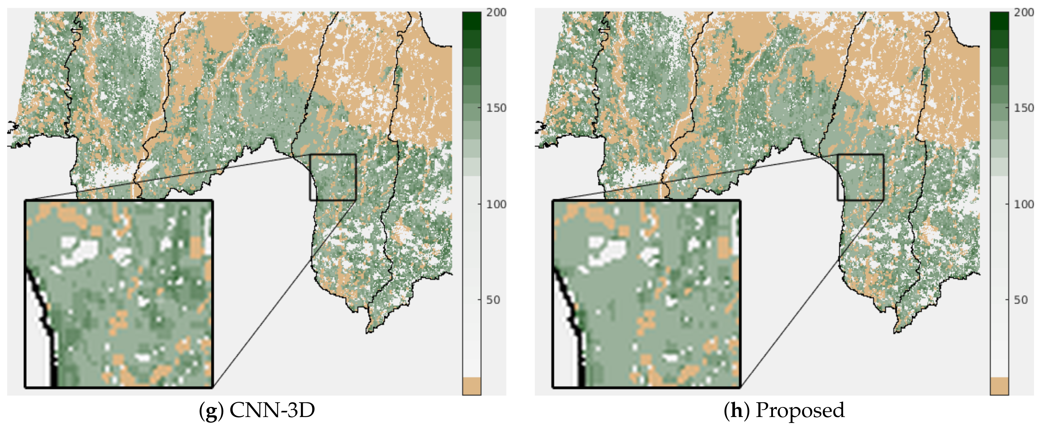
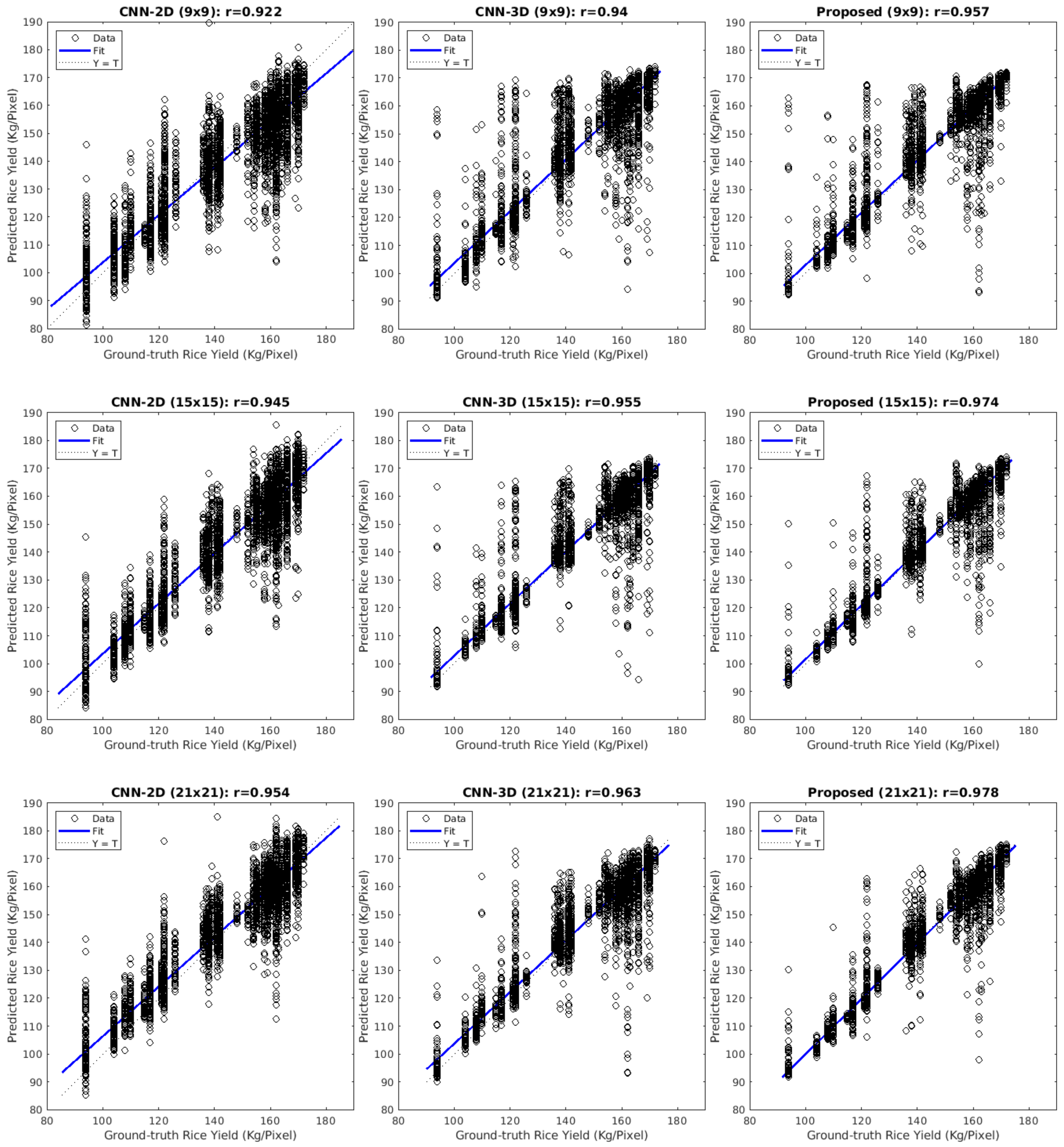
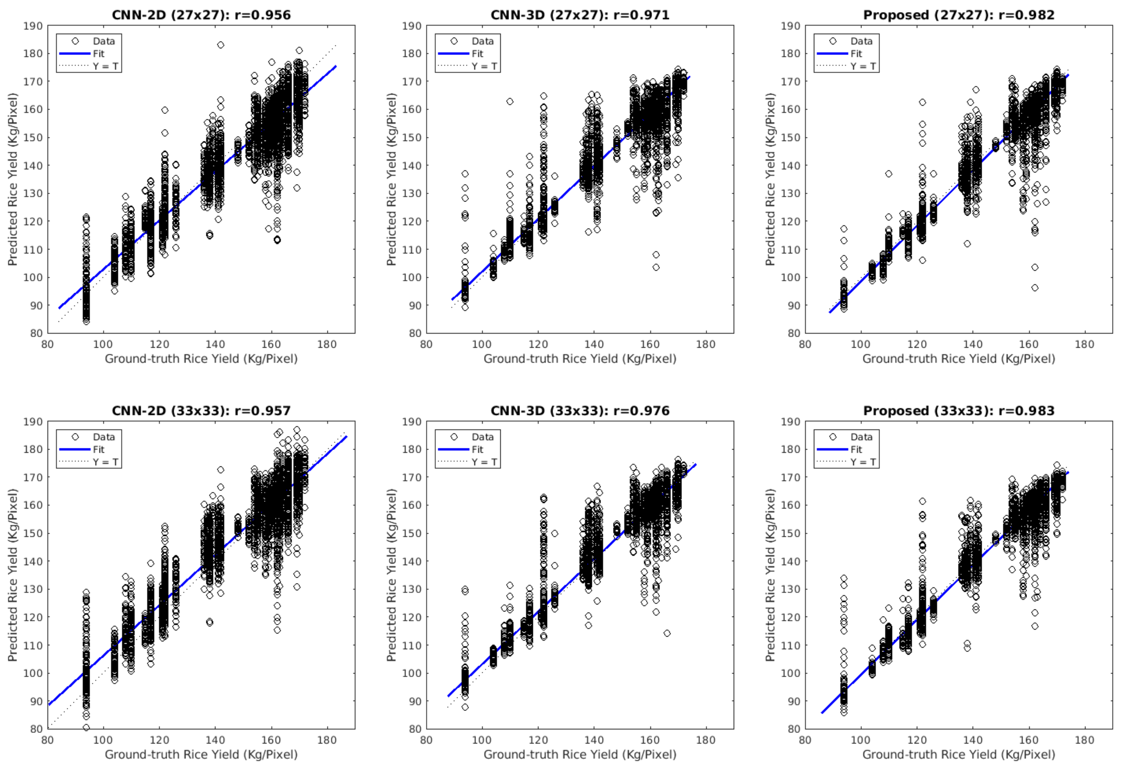
Table 1.
Data sources considered for building the RicePAL dataset.
| Data | Source | |
|---|---|---|
| Sentinel-2 | B02-B08, B8A, B11, and B12 | https://scihub.copernicus.eu/ accessed on 3 April 2021 |
| NDVI | Calculated using bands B04 and B08 | |
| Cloud mask | Available with L1C products | |
| Auxiliary | Climate | https://www.dhm.gov.np/ accessed on 3 April 2021 |
| Soil | https://krishiprabidhi.net/ accessed on 3 April 2021 | |
| Ground-truth | Rice crop mask | Based on Qamer et al. [39] |
| Rice crop yield | https://mold.gov.np/ accessed on 3 April 2021 | |
Table 2.
Climate data included in RicePAL.
| Climate Variables | Unit |
|---|---|
| Rainfall | Millimeter (mm) |
| Maximum temperature | Degree Celsius () |
| Minimum temperature | Degree Celsius () |
| Relative Humidity | Percentage (%) |
Table 3.
Experiment 1: Quantitative results in terms of root mean squared error (RMSE) (kg/ha). In rows, the considered data combinations, where S/P/E-S2 represents S2 images of start/peak/end of rice season. In columns, the methods considered for the rice yield estimation, including traditional regression algorithms, CNN-based and proposed network with different patch sizes.
| DATA | LIN | RID | SVR | GPR | CNN-2D | CNN-3D | Proposed | ||||||||||||
|---|---|---|---|---|---|---|---|---|---|---|---|---|---|---|---|---|---|---|---|
| 9 | 15 | 21 | 27 | 33 | 9 | 15 | 21 | 27 | 33 | 9 | 15 | 21 | 27 | 33 | |||||
| S-S2 | 495.24 | 503.33 | 456.35 | 438.33 | 332.87 | 294.45 | 265.43 | 271.26 | 235.47 | 410.89 | 348.73 | 319.38 | 311.77 | 283.12 | 287.34 | 255.97 | 217.55 | 192.12 | 170.16 |
| P-S2 | 529.26 | 534.71 | 462.29 | 442.86 | 370.34 | 343.60 | 305.64 | 314.96 | 310.22 | 412.47 | 372.55 | 336.13 | 365.40 | 323.37 | 339.35 | 282.32 | 214.32 | 215.80 | 215.71 |
| E-S2 | 532.75 | 540.30 | 481.50 | 465.38 | 340.29 | 319.86 | 285.41 | 256.32 | 252.94 | 413.85 | 314.87 | 288.36 | 272.97 | 234.54 | 278.80 | 201.19 | 247.31 | 158.53 | 160.67 |
| S/P-S2 | 480.22 | 492.34 | 386.30 | 370.18 | 251.60 | 224.61 | 207.30 | 206.76 | 198.93 | 261.15 | 199.06 | 184.32 | 166.64 | 163.27 | 188.97 | 140.40 | 121.85 | 114.80 | 115.96 |
| P/E-S2 | 512.42 | 526.10 | 419.01 | 408.46 | 295.89 | 227.63 | 211.20 | 223.45 | 178.12 | 264.48 | 223.83 | 199.49 | 176.52 | 179.84 | 202.18 | 147.00 | 134.33 | 127.03 | 117.97 |
| S/E-S2 | 482.01 | 497.63 | 393.40 | 389.02 | 238.63 | 213.19 | 176.69 | 176.03 | 168.83 | 265.99 | 230.56 | 198.44 | 156.82 | 151.91 | 169.52 | 182.02 | 106.65 | 116.26 | 117.20 |
| S/P/E-S2 | 468.30 | 487.37 | 359.51 | 349.14 | 216.24 | 187.95 | 168.32 | 157.00 | 158.90 | 215.42 | 174.37 | 162.82 | 123.60 | 115.96 | 181.77 | 119.38 | 117.84 | 103.80 | 89.03 |
| Avg. | 500.03 | 511.68 | 422.62 | 409.05 | 292.27 | 258.76 | 231.43 | 229.40 | 214.77 | 320.61 | 266.28 | 241.28 | 224.82 | 207.43 | 235.42 | 189.75 | 165.69 | 146.91 | 140.96 |
Table 4.
Experiment 2: Quantitative results in terms of RMSE (kg/ha), where +C indicates adding auxiliary climate data.
Table 4.
Experiment 2: Quantitative results in terms of RMSE (kg/ha), where +C indicates adding auxiliary climate data.
| DATA | LIN | RID | SVR | GPR | CNN-2D | CNN-3D | Proposed | ||||||||||||
|---|---|---|---|---|---|---|---|---|---|---|---|---|---|---|---|---|---|---|---|
| 9 | 15 | 21 | 27 | 33 | 9 | 15 | 21 | 27 | 33 | 9 | 15 | 21 | 27 | 33 | |||||
| S-S2+C | 485.56 | 496.50 | 439.26 | 432.87 | 336.85 | 296.08 | 280.71 | 270.69 | 261.94 | 431.73 | 363.31 | 306.86 | 275.56 | 267.95 | 297.90 | 253.40 | 253.59 | 206.93 | 174.14 |
| P-S2+C | 515.11 | 521.01 | 447.23 | 430.08 | 379.00 | 336.51 | 295.16 | 305.76 | 324.00 | 431.39 | 388.09 | 353.88 | 332.59 | 297.94 | 329.11 | 310.26 | 254.31 | 240.12 | 223.17 |
| E-S2+C | 530.89 | 538.30 | 465.35 | 456.47 | 349.84 | 300.20 | 247.51 | 251.86 | 240.66 | 380.69 | 360.55 | 304.01 | 340.33 | 243.33 | 302.22 | 265.71 | 201.16 | 198.38 | 179.44 |
| S/P-S2+C | 470.92 | 485.13 | 380.21 | 376.56 | 289.66 | 235.30 | 215.59 | 195.79 | 187.61 | 276.73 | 231.51 | 201.26 | 172.41 | 168.97 | 171.48 | 179.83 | 140.46 | 132.57 | 138.87 |
| P/E-S2+C | 488.04 | 501.99 | 398.19 | 399.14 | 277.58 | 240.85 | 200.47 | 216.91 | 193.91 | 298.59 | 222.10 | 214.16 | 170.12 | 162.96 | 197.40 | 163.29 | 159.53 | 136.89 | 157.19 |
| S/E-S2+C | 465.73 | 482.20 | 379.82 | 371.43 | 248.35 | 212.57 | 178.93 | 182.06 | 171.85 | 260.58 | 200.27 | 186.53 | 169.67 | 161.05 | 164.65 | 185.40 | 127.87 | 105.39 | 114.25 |
| S/P/E-S2+C | 452.90 | 473.06 | 346.14 | 336.34 | 212.12 | 193.83 | 214.40 | 194.49 | 181.20 | 190.95 | 216.35 | 159.52 | 131.16 | 113.47 | 159.12 | 120.56 | 122.95 | 156.41 | 107.69 |
| Avg. | 487.02 | 499.74 | 408.03 | 400.41 | 299.06 | 259.33 | 233.25 | 231.08 | 223.02 | 324.38 | 283.17 | 246.60 | 227.41 | 202.24 | 231.70 | 211.21 | 179.98 | 168.10 | 156.39 |
Table 5.
Experiment 3: Quantitative results in terms of RMSE (kg/ha), where +S indicates adding auxiliary soil data.
Table 5.
Experiment 3: Quantitative results in terms of RMSE (kg/ha), where +S indicates adding auxiliary soil data.
| DATA | LIN | RID | SVR | GPR | CNN-2D | CNN-3D | Proposed | ||||||||||||
|---|---|---|---|---|---|---|---|---|---|---|---|---|---|---|---|---|---|---|---|
| 9 | 15 | 21 | 27 | 33 | 9 | 15 | 21 | 27 | 33 | 9 | 15 | 21 | 27 | 33 | |||||
| S-S2+S | 495.15 | 503.16 | 447.32 | 430.88 | 332.08 | 293.20 | 287.92 | 254.69 | 236.77 | 411.11 | 329.71 | 313.52 | 301.75 | 272.50 | 299.93 | 234.14 | 206.71 | 191.80 | 188.58 |
| P-S2+S | 529.17 | 534.60 | 455.64 | 446.67 | 377.25 | 359.96 | 317.79 | 319.12 | 324.43 | 396.86 | 358.92 | 338.78 | 330.88 | 295.28 | 311.55 | 271.84 | 231.51 | 240.32 | 218.29 |
| E-S2+S | 532.56 | 540.16 | 476.87 | 467.09 | 358.70 | 312.74 | 270.84 | 237.39 | 225.53 | 411.98 | 330.43 | 305.51 | 270.15 | 255.74 | 302.53 | 221.49 | 192.84 | 198.88 | 165.13 |
| S/P-S2+S | 480.41 | 492.48 | 379.55 | 382.08 | 250.64 | 247.28 | 205.30 | 202.43 | 214.76 | 261.63 | 211.86 | 206.61 | 173.77 | 165.89 | 200.38 | 163.96 | 148.50 | 130.75 | 94.19 |
| P/E-S2+S | 512.35 | 526.07 | 417.70 | 408.12 | 274.77 | 295.89 | 221.70 | 231.88 | 259.55 | 275.95 | 216.97 | 197.82 | 169.72 | 159.86 | 199.36 | 170.12 | 134.63 | 123.04 | 140.72 |
| S/E-S2+S | 481.89 | 497.52 | 386.97 | 383.77 | 273.69 | 250.01 | 248.09 | 171.57 | 200.49 | 245.98 | 184.04 | 193.61 | 165.58 | 145.45 | 182.61 | 126.60 | 115.58 | 120.51 | 99.95 |
| S/P/E-S2+S | 468.49 | 487.37 | 356.67 | 348.40 | 251.79 | 199.39 | 167.91 | 171.83 | 165.26 | 208.29 | 167.74 | 136.63 | 137.61 | 107.26 | 172.25 | 131.74 | 145.81 | 96.89 | 115.95 |
| Avg. | 500.00 | 511.62 | 417.25 | 409.57 | 302.70 | 279.78 | 245.65 | 226.99 | 232.40 | 315.97 | 257.10 | 241.78 | 221.35 | 200.28 | 238.37 | 188.56 | 167.94 | 157.46 | 146.11 |
Table 6.
Experiment 4: Quantitative results in terms of RMSE (kg/ha).
| DATA | LIN | RID | SVR | GPR | CNN-2D | CNN-3D | Proposed | ||||||||||||
|---|---|---|---|---|---|---|---|---|---|---|---|---|---|---|---|---|---|---|---|
| 9 | 15 | 21 | 27 | 33 | 9 | 15 | 21 | 27 | 33 | 9 | 15 | 21 | 27 | 33 | |||||
| S-S2+C+S | 485.62 | 496.54 | 438.00 | 431.88 | 334.85 | 309.86 | 275.38 | 269.76 | 240.92 | 445.60 | 375.98 | 335.11 | 292.70 | 270.40 | 292.13 | 255.26 | 220.48 | 186.67 | 196.91 |
| P-S2+C+S | 515.17 | 521.03 | 442.93 | 436.52 | 365.72 | 377.89 | 312.69 | 309.62 | 289.73 | 406.37 | 368.45 | 344.81 | 328.45 | 296.09 | 333.73 | 318.97 | 263.84 | 223.47 | 236.45 |
| E-S2+C+S | 530.65 | 538.09 | 463.05 | 453.01 | 326.07 | 296.11 | 258.14 | 249.32 | 252.56 | 373.47 | 358.05 | 294.38 | 319.73 | 269.55 | 293.80 | 255.81 | 203.88 | 188.81 | 190.90 |
| S/P-S2+C+S | 471.21 | 485.20 | 374.12 | 363.00 | 250.07 | 237.04 | 230.39 | 216.44 | 186.00 | 262.65 | 231.24 | 212.40 | 188.13 | 176.68 | 175.25 | 185.50 | 167.74 | 135.69 | 133.02 |
| P/E-S2+C+S | 488.30 | 502.02 | 398.57 | 394.72 | 270.10 | 211.63 | 207.69 | 228.69 | 227.35 | 260.76 | 207.65 | 202.63 | 191.30 | 169.11 | 201.04 | 162.45 | 155.18 | 131.43 | 145.19 |
| S/E-S2+C+S | 465.93 | 482.30 | 375.80 | 369.94 | 271.27 | 207.56 | 176.92 | 177.63 | 188.86 | 262.06 | 199.32 | 201.29 | 186.16 | 161.08 | 176.23 | 138.77 | 119.00 | 126.32 | 109.39 |
| S/P/E-S2+C+S | 453.30 | 473.33 | 345.97 | 339.85 | 230.09 | 183.46 | 167.45 | 181.84 | 165.45 | 189.95 | 163.66 | 147.56 | 132.14 | 120.91 | 159.29 | 125.54 | 117.50 | 113.50 | 108.49 |
| Avg. | 487.17 | 499.79 | 405.49 | 398.42 | 292.60 | 260.51 | 232.67 | 233.33 | 221.55 | 314.41 | 272.05 | 248.31 | 234.09 | 209.12 | 233.07 | 206.04 | 178.23 | 157.98 | 160.05 |
Table 7.
Summary with the best RMSE (kg/ha) result for each experiment and method.
| EXPERIMENTS | LIN | RID | SVR | GPR | CNN-2D | CNN-3D | Proposed | ||||||||||||
|---|---|---|---|---|---|---|---|---|---|---|---|---|---|---|---|---|---|---|---|
| 9 | 15 | 21 | 27 | 33 | 9 | 15 | 21 | 27 | 33 | 9 | 15 | 21 | 27 | 33 | |||||
| Experiment 1 | 468.30 | 487.37 | 359.51 | 349.14 | 216.24 | 187.95 | 168.32 | 157.00 | 158.90 | 215.42 | 174.37 | 162.82 | 123.60 | 115.96 | 169.52 | 119.38 | 106.65 | 103.80 | 89.03 |
| Experiment 2 | 452.90 | 473.06 | 346.14 | 336.34 | 212.12 | 193.83 | 178.93 | 182.06 | 171.85 | 190.95 | 200.27 | 159.52 | 131.16 | 113.47 | 159.12 | 120.56 | 122.95 | 105.39 | 107.69 |
| Experiment 3 | 468.49 | 487.37 | 356.67 | 348.40 | 250.64 | 199.39 | 167.91 | 171.57 | 165.26 | 208.29 | 167.74 | 136.63 | 137.61 | 107.26 | 172.25 | 126.60 | 115.58 | 96.89 | 94.19 |
| Experiment 4 | 453.30 | 473.33 | 345.97 | 339.85 | 230.09 | 183.46 | 167.45 | 177.63 | 165.45 | 189.95 | 163.66 | 147.56 | 132.14 | 120.91 | 159.29 | 125.54 | 117.50 | 113.50 | 108.49 |
| Best | 452.90 | 473.06 | 345.97 | 336.34 | 212.12 | 183.46 | 167.45 | 157.00 | 158.90 | 189.95 | 163.66 | 136.63 | 123.60 | 107.26 | 159.12 | 119.38 | 106.65 | 96.89 | 89.03 |
Publisher’s Note: MDPI stays neutral with regard to jurisdictional claims in published maps and institutional affiliations. |
© 2021 by the authors. Licensee MDPI, Basel, Switzerland. This article is an open access article distributed under the terms and conditions of the Creative Commons Attribution (CC BY) license (https://creativecommons.org/licenses/by/4.0/).
Share and Cite
MDPI and ACS Style
Fernandez-Beltran, R.; Baidar, T.; Kang, J.; Pla, F. Rice-Yield Prediction with Multi-Temporal Sentinel-2 Data and 3D CNN: A Case Study in Nepal. Remote Sens. 2021, 13, 1391. https://0-doi-org.brum.beds.ac.uk/10.3390/rs13071391
AMA Style
Fernandez-Beltran R, Baidar T, Kang J, Pla F. Rice-Yield Prediction with Multi-Temporal Sentinel-2 Data and 3D CNN: A Case Study in Nepal. Remote Sensing. 2021; 13(7):1391. https://0-doi-org.brum.beds.ac.uk/10.3390/rs13071391
Chicago/Turabian StyleFernandez-Beltran, Ruben, Tina Baidar, Jian Kang, and Filiberto Pla. 2021. "Rice-Yield Prediction with Multi-Temporal Sentinel-2 Data and 3D CNN: A Case Study in Nepal" Remote Sensing 13, no. 7: 1391. https://0-doi-org.brum.beds.ac.uk/10.3390/rs13071391
Note that from the first issue of 2016, this journal uses article numbers instead of page numbers. See further details here.