Machine Learning Optimised Hyperspectral Remote Sensing Retrieves Cotton Nitrogen Status

Abstract

Hyperspectral imaging spectrometers mounted on unmanned aerial vehicle (UAV) can capture high spatial and spectral resolution to provide cotton crop nitrogen status for precision agriculture. The aim of this research was to explore machine learning use with hyperspectral datacubes over agricultural fields. Hyperspectral imagery was collected over a mature cotton crop, which had high spatial (~5.2 cm) and spectral (5 nm) resolution over the spectral range 475–925 nm that allowed discrimination of individual crop rows and field features as well as a continuous spectral range for calculating derivative spectra. The nominal reflectance and its derivatives clearly highlighted the different treatment blocks and were strongly related to N concentration in leaf and petiole samples, both in traditional vegetation indices (e.g., Vogelman 1, R² = 0.8) and novel combinations of spectra (R² = 0.85). The key hyperspectral bands identified were at the red-edge inflection point (695–715 nm). Satellite multispectral was compared against the UAV hyperspectral remote sensing’s performance by testing the ability of Sentinel MSI to predict N concentration using the bands in VIS-NIR spectral region. The Sentinel 2A Green band (B3; mid-point 559.8 nm) explained the same amount of variation in N as the hyperspectral data and more than the Sentinel Red Edge Point 1 (B5; mid-point 704.9 nm) with the lower 10 m resolution Green band reporting an R² = 0.85, compared with the R² = 0.78 of downscaled Sentinel Red Edge Point 1 at 5 m. The remaining Sentinel bands explained much lower variation (maximum was NIR at R² = 0.48). Investigation of the red edge peak region in the first derivative showed strong promise with RIDAmid (R² = 0.81) being the best index. The machine learning approach narrowed the range of bands required to investigate plant condition over this trial site, greatly improved processing time and reduced processing complexity. While Sentinel performed well in this comparison and would be useful in a broadacre crop production context, the impact of pixel boundaries relative to a region of interest and coarse spatial and temporal resolution impacts its utility in a research capacity.

1. Introduction

Being able to remotely and rapidly identify the nitrogen level in plants and tailor farm management to either boost higher yield potential zones or reduce inputs to lower potential areas promises a way to reduce environmental impact while increasing profits. Nitrogen is a key nutrient in cotton (Gossypium hirsutum L.), essential for photosynthesis and thus undersupply will hamper lint and seed production, while oversupply can damage local ecosystems and adversely affect yield [1,2,3,4]. It’s been widely reported for decades that nitrate leaching into the groundwater [5] and emission as oxides into the atmosphere [6] cause extensive local and global environmental damage, with, for example, intensive agriculture in the USA contributing to ~400 hypoxic zones in coastal marine ecosystems from farms upstream [7]. Within the cotton industry, lint yields have increased through improved plant genetics and management, however, there is a need to investigate ways to improve nitrogen use efficiency as yield quantities are not uniformly responsive to the high levels of N applied [8]. By identifying N concentration spatially across a cotton crop the factors influencing N use efficiency can be studied, leading to more tailored N management strategies.

Radiation reflected from crop canopies is controlled by leaf biochemical composition and physical structure, canopy density, soil and environmental background, and can give important insights into plant condition [9,10,11]. The spectral feature in the region between the chlorophyll absorption well of the red band (670 nm) and thermal reflection peak of the Near Infra-Red band (NIR; 800 nm) is commonly referred to as the red edge and is of great interest for N detection due to leaf status influencing where and what shape this transition takes [12,13,14]. The curve of vegetation reflectance in the red edge region exhibits shifts to either shorter or longer wavelengths depending on plant condition [1]. Shifts of the curve in the spectral region around 720 nm to shorter wavelengths, or ‘blue shifts’, have been found to be associated with reduced plant vigour, while ‘red shifts’ to longer wavelengths can be related with strong growth [15,16]. One theory for this change in position is that stronger vigour is related to higher chlorophyll content, which increases absorption around the red region, thus widening the absorption well and shifting the curve to absorb more energy in longer wavelengths [17]. This is an area of substantial long-term research, however, there are a number of studies showing that the red edge position is impacted by multiple sources, such as water content, salinity and leaf solar geometry, with some divergent results encountered across different studies [14,17,18,19]. The geometry of the crop surface in the region of interest in relation to both the sun and viewing sensor zenith (vertical) and azimuth (horizontal) angles also has nonlinear impacts on the reflectance received at the sensor, referred to as the bi-directional reflectance distribution function (BRDF) [20].

Remote sensing detection of canopy condition in the visible to near infrared spectral region uses two broad categories of instruments: multispectral and hyperspectral. Multispectral sensors capture discrete spectral regions centred on specific wavelengths, principally in the blue (centred at 475 nm), green (560 nm), red, red edge (715 nm), and NIR, though the central wavelength, field of view and the width of the spectral region captured at each band varies across instruments [21,22]. Hyperspectral sensors record continuous spectra over the visible to thermal domain, with the spectral resolution, field of view, range and whether they capture point spectrometry or imagery depending on the instrument [23]. Remote sensing investigation of nitrogen with hyperspectral instruments in cotton has focused mostly on ground-based point sampling, essentially spectroscopy [24,25,26,27,28]. There have also been studies using multispectral instruments on airborne (unmanned and manned aircraft) and satellite platforms for phenology [29,30], yield variability [31,32] and pest detection [33]. In other crops, such as wheat, there is significant research in using hyperspectral imager sensors rather than point-based sampling to detect canopy reflectance variation across a continuous spectral range and large areas rapidly [34]. The higher spatial and spectral resolution can characterise individual plant features useful for implementing precision agriculture, as well as reducing the mixed pixel effects that impacts coarse resolution sensors mounted on satellites [35].

The majority of agricultural remote sensing users apply vegetation indices (VIs) of nominal reflectance values to infer plant status, including the normalised difference vegetation index (NDVI) [36], normalised difference red edge (NDRE) [37], Vogelman 1 (VOG1) [38], canopy chlorophyll content index (CCCI) [39], the ratio of transformed chlorophyll absorption in reflectance index to the optimised soil adjusted vegetation index (TCARI/OSAVI) [40], and the modified normalised difference in red edge index (mND705) [19]. These incorporate different band combinations to highlight different plant conditions or minimise the impact of background sources of reflectance. For example, normalised difference red edge was developed to use the red edge region rather than red to minimise the impact of canopy density and improve characterisation of chlorophyll content [10,37]. There is a high correlation between chlorophyll content and N concentration in cotton canopy leaves, most likely because the main pigments used in photosynthesis in the chloroplasts, chlorophyll a and b, contain N [4,28,41].

The reflectance curve, defined by the proportion of received radiance that is reflected back to the sensor at each wavelength, describes one component (along with transmission and absorption) of the response of a plant canopy to incoming solar radiation, with higher or lower reflectance in different spectral regions controlled by plant and sensing conditions. There has been a large body of research using handheld spectroradiometers to maximise information about the rate of change and intensity of spectral features to identify N levels through first derivative spectra and areal measures [9,12,13]. These characterise the slope of the reflectance curve at each wavelength and the sum of reflectance over particular regions, respectively [13,42]. Early interest in derivative spectra was mainly focused on identifying the red edge inflection point for multispectral satellite data [43,44], though more recent research suggests there is potential for derivatives to improve characterisation of photosynthetic processes that may be resistant to species and soil background variability [45]. Comparing derivative spectra and leaf N content in wheat, Feng et al. (2014) found the derivative indices which incorporated information on the double peak evident in some species’ derivative curves were more stable and had lower error in N prediction than either the commonly used red edge or other derivative VIs. The key derivative VIs were found to be the left side double-peak area of the red edge region (LSDR), measuring the sum of the derivative spectra on the ascending side of the peak; the right side double-peak area of the red edge region (RSDR), using the sum of the descending side; ratio index double-peak area (RIDA), taking the ratio of RSDR and LSDR; the difference index of double-peak areas (DIDA), difference between LSDR and RSDR; and the normalised difference double-peak Area (NDDA), the DIDA normalised by the sum of the full peak [13].

Satellites offer a way for production-scale agriculture to leverage the ability of remote sensing to characterise N variability across a crop canopy. Sentinel 2 was launched in 2015 and 2017 and consists of 2 satellites operating in a sun-synchronous orbit allowing revisit times of 5 days, each carrying a single multi-spectral instrument (MSI) with a swath width of 60 km and spatial resolution of 10–20 m for the VIS, red-edge (RE), and NIR bands [46]. Sentinel data has been extensively used over crops to assess vegetation health and biochemical constituents [47,48,49,50,51,52]. The coarse spatial resolution of many satellite sensors has been a limiting factor for their use in some agricultural applications, with the inclusion of features with differing spectral characteristics within a single pixel, or mixed-pixels, impacting reported reflectance [53].

With the rise in computer processor speed and capacity as well as available observation data streams, supervised and unsupervised learning methods, collectively referred to as machine learning, have seen increasing use in agricultural remote sensing applications since 2010 [18]. There are a large number of techniques in use, with many of these reviewed by Verrelst et al. (2015). Clustering is a classification approach that groups similar samples together and can be used to identify reflectance bands that covary, especially after dimension reduction using principal component analysis (PCA). PCA can be defined as the orthogonal projection of data onto a lower dimensional space to maximise the variance of the projected dataset and is one of the more commonly used techniques in remote sensing and machine learning [54]. Random forest regression is a form of non-linear non-parametric regression that uses a series of decision trees to assess relationship within the dataset; each tree consists of a series of binary decision nodes that minimise a sum of squares cost function to find the subsection of the dataset most related to the target variable [49]. Research combining remote sensing with various supervised and unsupervised feature detection, classification and prediction methods has been successfully used in varied agricultural contexts, such as leaf area index (LAI) detection in rice [55], regional baled fodder classification [56] and yield prediction [57]. Conversely, Féret et al. (2019) trained a support vector machine (SVM) to predict leaf mass area and equivalent water thickness and tested it against field data and a leaf optical model and found that the SVM lacked generality [58]. The contrast in reported performance suggests the need for large sample sizes to train machine learning models to predict target features from unseen data.

Therefore, this study investigates using machine learning to identify novel combinations of hyperspectral spectral features on a cotton canopy to detect N concentration. There were three main objectives: (i) to explore supervised and unsupervised learning methods for identifying hyperspectral regions responsive to variables of interest; (ii) to leverage these highlighted spectral regions in novel configurations of hyperspectral bands and test their ability to predict N concentration; and (iii), to compare a UAV-based hyperspectral against a satellite-based multispectral instrument for detecting cotton N concentration.

2. Materials and Methods

2.1. Study Site

The experimental site was in the north west of New South Wales (NSW), at the Australian Cotton Research Institute near Narrabri (see Figure 1). The main crops grown in the region are cotton and wheat. The predominant soil type in the region is a Vertosol and receives a mean annual rainfall of 592 mm with a mean maximum temperature during summer of 35 °C and a mean minimum during winter of 3 °C [59]. There were 10 plots of 30 m by 32 m with 3 replicates each of N treatments of 0, 200, and 400 kg ha⁻¹ applied at sowing. The site was irrigated so water was non-limiting.

2.2. Field Sampling

The field observations were each an average of 40 leaf and petiole samples from randomly selected plants around georeferenced points (~5 m accuracy), with 20 taken from plants around two pegs at each georeferenced point. There were three georeferenced points (A, B, and C) for each plot, giving 30 averaged samples from 1200 total field samples chemically analysed. The N concentration was tested in a commercial laboratory and confirmed in a LECO gas analyzer (CN928) onsite at ACRI with a R² of 0.90.

2.3. Hyperspectral Data Collection

Hyperspectral imagery was collected over a mature cotton stand on the 19 February 2019, under cloudless conditions with moderate winds (20–24 km/h), 36 C ambient temperature within 2 h of solar noon. Panels with known reflectance properties were laid out and ground control points were arranged around the edges of the region of interest with their locations measured with a Trimble R2 Integrated Global Navigation Satellite System (GNSS) Differential Global Positioning System (DGPS) unit (~2 cm accuracy). The hyperspectral instrument was a Cubert ButterflEYE LS S199 imaging sensor utilising a linear filter on chip design providing 2-megapixel sensor resolution using a Si CMOS detector with 5–10 nm spectral resolution (interpolated down to 5 nm) over the VIS to NIR region (475 to 925 nm). The sensor was mounted on a DJI Matrice M600 UAV with RTK link provided by DJI DataLink Pro 900-G. The flight was conducted at 50 m altitude, with 1.6 m s⁻¹ speed with a fixed roughly sunward orientation along the flight path. Camera settings were 20 Hz frame rate and 2 ms integration. Due to the prevailing heat and slow speed, there were battery changes during the flight that resulted in two flight missions being separately orthomosaicked and radiometrically corrected by an external provider (Vito, Belgium) using panels with known reflectance positioned within the imagery. The imagery of the two missions were stitched, reprojected and scaled radiometrically, then single pixel and 20 cm areal average reflectance vectors were taken at 30 sample points matching the field data.

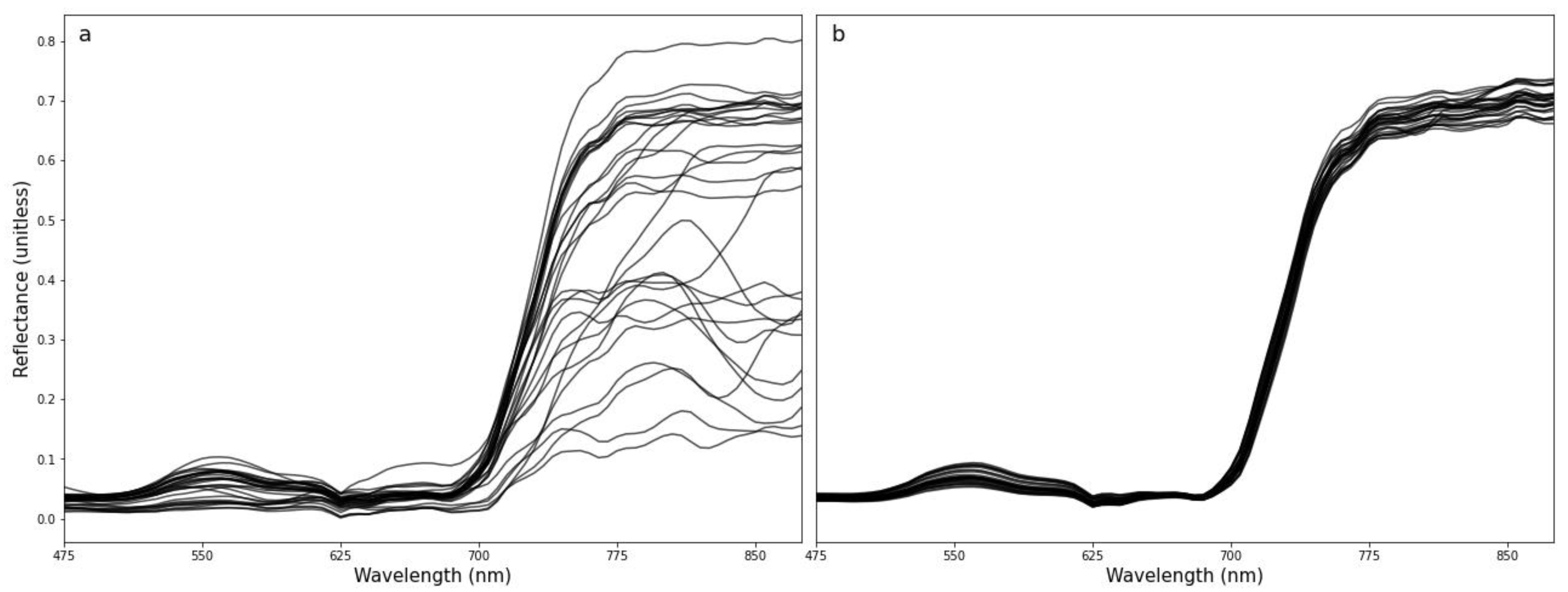
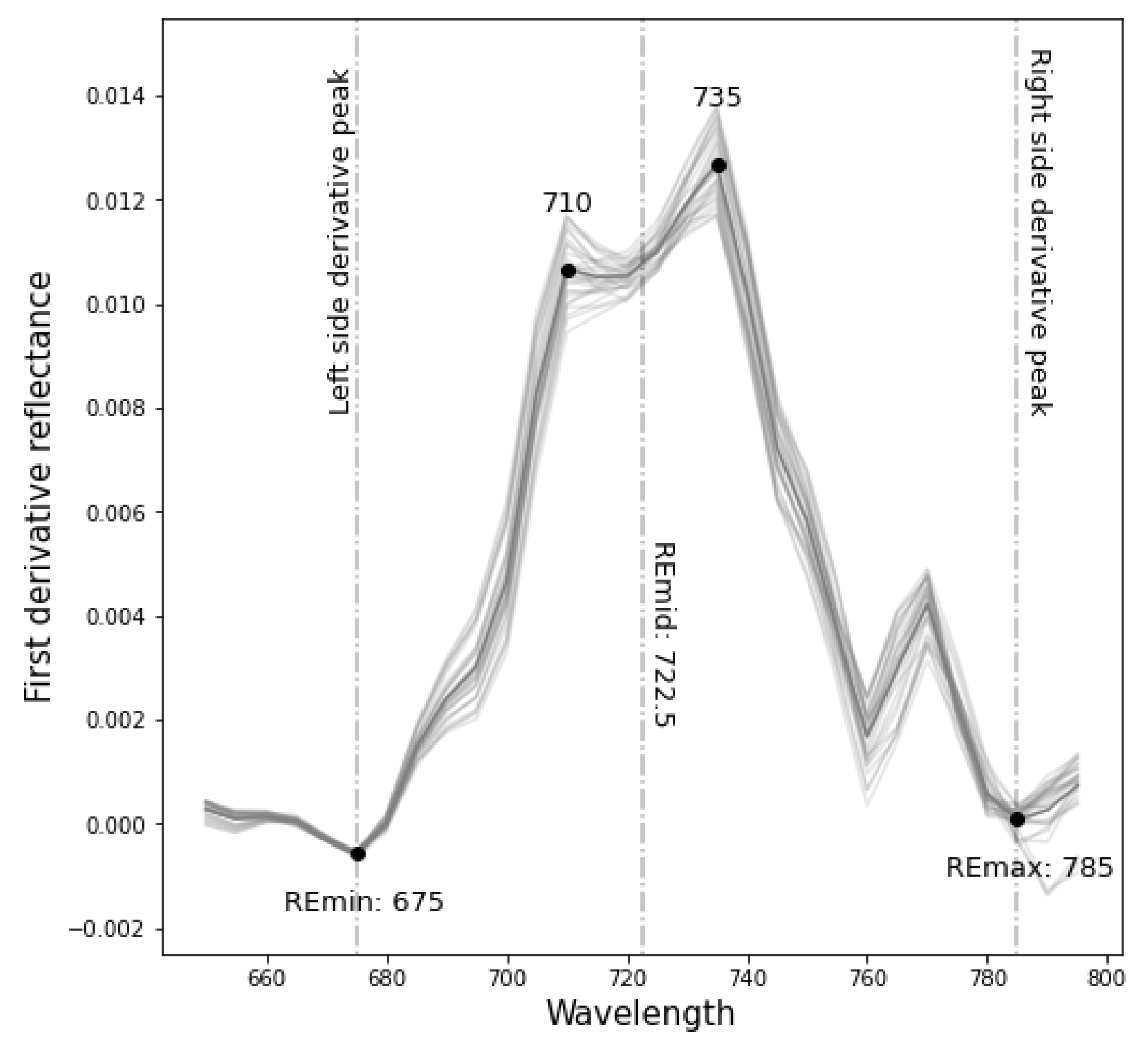
2.4. Hyperspectral Derivatives Extraction

First derivatives were calculated using first order difference as per:

$$\frac{dR}{d\lambda }=\frac{\left(R_{\lambda \left(j+1\right)}-R_{\lambda \left(j\right)}\right)}{\delta \lambda }$$

(1)

where R is the reflectance at λ wavelength, ordered by j = 1 … n and δλ is the bandwidth between wavelengths (5 nm in this dataset). The first derivative was smoothed with a filter using a 2nd order polynomial and 5 band fitting window [60].

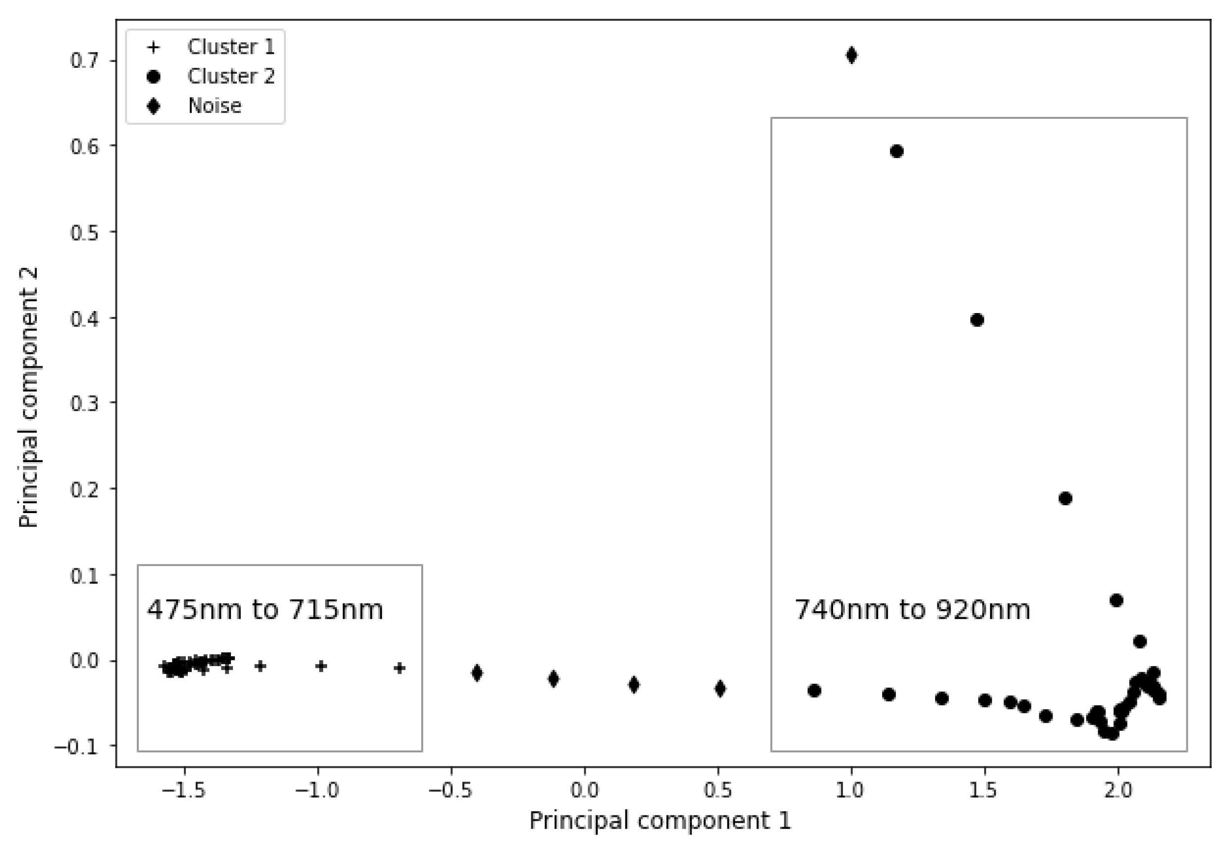
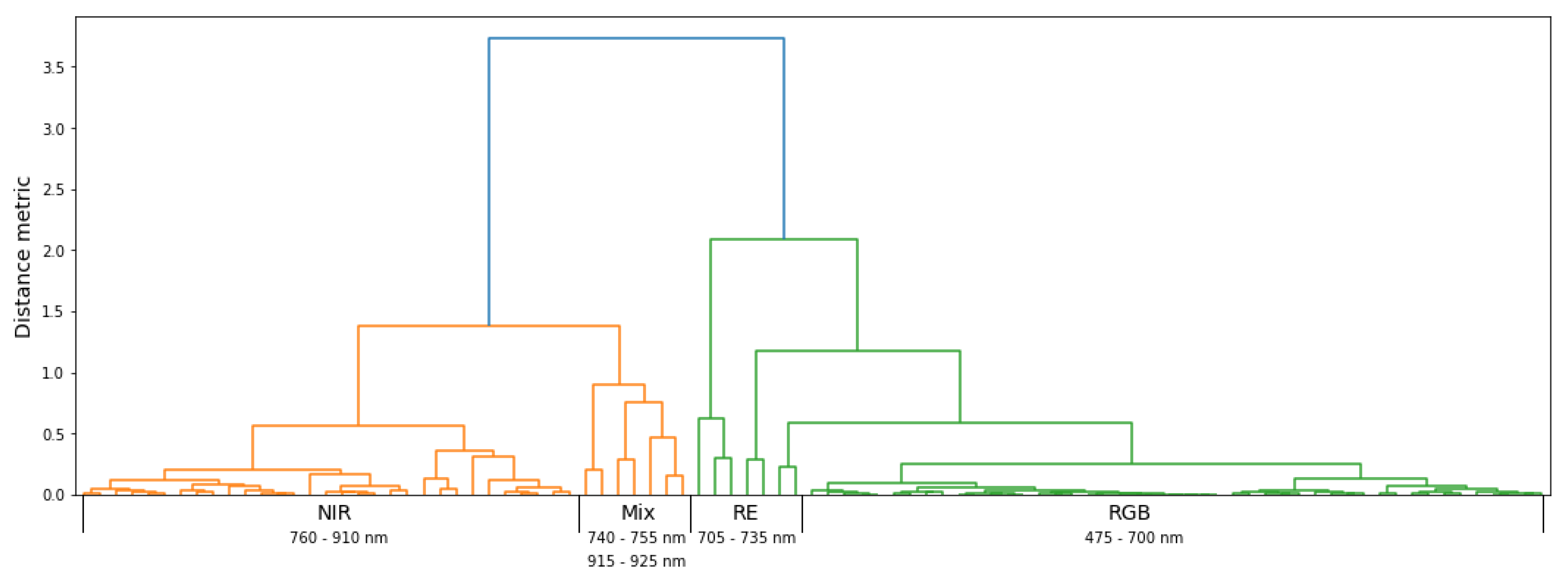
2.5. Machine Learning Classification on the Hyperspectral Datacube

Nominal and derivative reflectance values were investigated using density-based and hierarchical clustering, and Random Forest regression to identify the most important bands for discriminating N content. Density Based spatial clustering of applications with noise (DBSCAN) method was employed after decomposing the average areal reflectance into 4 principal components using principal component analysis (PCA) and plotted using the 2 that explained the most variance. DBSCAN groups samples of unlabelled data into clusters of high density (those with many neighbours), and noise (those samples with few or no neighbours) [61]. The hierarchical clustering was processed using an agglomerative complete linkage approach, which starts with all samples in individual clusters and then groups them based on minimising a Euclidean distance metric [62]. Sets of spectral bands covering the full range (91), the top 15 and the top 10 in Random Forest returned feature importance were trained against the labelled N concentration to find those which had the lowest residual sum of squares. The random forest regressor had a maximum depth of 3 levels and used a random 30% of the dataset (rounded down) at each split. The most important bands identified in the unsupervised and supervised learning were then iteratively combined and assessed against the N samples using ordinary least squares with leave one out cross validation as with the hyperspectral dataset. Using a sum, product and difference ratio configuration, there were 3000 possible combinations of the 10 bands, however, 300 were dropped to avoid repeating the same band in the numerator. Combinations with R² > 0.40 were retained for review. This was done for both the nominal and derivative reflectance. Due to the small sample size and non-repeated measures, machine learning was used only to identify the optimal reflectance region rather than incorporated into the modelling.

2.6. Common Vegetation Indices Calculation

To compare the UAV hyperspectral and satellite spectral response with other remote sensing approaches, a selection of vegetation indices used in the literature for identifying nitrogen or chlorophyll content variability were calculated from the averaged hyperspectral reflectance as per

Table 1. Vegetation indices used for discriminating N or chlorophyll content.

Name	Equation	Source
NDVI	$\frac{R_{800}-R_{670}}{R_{800}+R_{670}}$	[36]
NDRE	$\frac{R_{790}-R_{720}}{R_{790}+R_{720}}$	[37]
VOG1	$\frac{R_{740}}{R_{720}}$	[38]
CCCI	$\frac{\frac{R_{790}-R_{720}}{R_{790}+R_{720}}}{\frac{R_{800}-R_{670}}{R_{800}+R_{670}}}$	[39]
$\frac{\mathrm{TCARI}}{\mathrm{OSAVI}}$	$\frac{3\left[\left(R_{700}-R_{670}\right)-0.2\left(R_{700}-R_{550}\right)\frac{R_{700}}{R_{670}}\right]}{\frac{1.16\left(R_{800}-R_{670}\right)}{\left(R_{800}+R_{670}+0.16\right)}}$	[40]
mND705	$\frac{R_{750}-R_{705}}{R_{750}+R_{705}-2\left(R_{475}\right)}$	[19]
NDDAmid	$\frac{\left({\int }_{REmid}^{REmax}\frac{dR\mathsf{\lambda }}{d\mathsf{\lambda }}d\mathsf{\lambda }-{\int }_{\mathrm{REmin}}^{REmid}\frac{dR\mathsf{\lambda }}{d\mathsf{\lambda }}d\mathsf{\lambda }\right)}{{\int }_{REmin}^{REmax}\frac{dR\mathsf{\lambda }}{d\mathsf{\lambda }}d\mathsf{\lambda }}$	[13]
DIDAmid	${\int }_{REmid}^{REmax}\frac{dR\mathsf{\lambda }}{d\mathsf{\lambda }}d\mathsf{\lambda }-{\int }_{REmin}^{REmid}\frac{dR\mathsf{\lambda }}{d\mathsf{\lambda }}d\mathsf{\lambda }$	[13]
RIDAmid	$\frac{{\int }_{REmid}^{REmax}\frac{dR\mathsf{\lambda }}{d\mathsf{\lambda }}d\mathsf{\lambda }}{{\int }_{REmin}^{REmid}\frac{dR\mathsf{\lambda }}{d\mathsf{\lambda }}d\mathsf{\lambda }}$	[13]
LSDRmid	${\int }_{REmin}^{REmid}\frac{dR\mathsf{\lambda }}{d\mathsf{\lambda }}d\mathsf{\lambda }$	[13]
RSDRmid	${\int }_{REmid}^{REmax}\frac{dR\mathsf{\lambda }}{d\mathsf{\lambda }}d\mathsf{\lambda }$	[13]

. All VIs have the same GSD of 5.2 cm. The mean derivative curve between 650 and 800 nm was assessed for troughs, to find the left (REmin) and right (REmax) side of the feature, and for peaks, to find the midpoint between the peaks (REmid). Further, to compare the best performing Sentinel 2 products against the hyperspectral datacube, the spectral region in the UAV imagery covered by the Green and Red Edge Position 1 bands (see Table 3) were averaged and tested against the field observed N concentration.

2.7. Sentinel 2 Data Extraction

For the satellite multispectral imagery, several platforms were investigated to find the highest spatial resolution available at or near the UAV data collection. Sentinel surface reflectance was downloaded through Google Earth Engine (image dataset: Copernicus/S2_SR) as the mean of two flights (13 and 23 February, 2019), one on either side of the hyperspectral flight [63]. Data were taken from the same orbit (23) to maintain consistent sensor geometry, without BRDF correction, and was filtered with a bitmask to exclude nonzero cloud and cirrus scenes. Each layer was sampled with the georeferenced shapefiles, downscaled to 5 m with nearest neighbour at download, while both the red edge and green bands were additionally downloaded in their native resolution (20 m and 10 m, respectively). Sentinel bands were combined to form the same VIs as the hyperspectral reflectance and tested against N concentration.

2.8. Analysis of Nitrogen Prediction

Both the hyperspectral and Sentinel data set were assessed in predicting leaf N concentration using ordinary least squares with leave one out cross validation. Results were compared using the coefficient of determination (2), root mean square error (3), and Lin’s concordance correlation coefficient (4):

$$R^2=\frac{{\sum }_i{\left(\widehat{y_i}-\overline{y}\right)}^2}{{\sum }_i{\left(y_i-\overline{y}\right)}^2}$$

(2)

$$RMSE=\sqrt{{\displaystyle \sum }_{i=1}^n\frac{{\left(\widehat{y_i}-y_i\right)}^2}{n}}$$

(3)

$$\mathrm{LCCC}=\frac{2\left(\frac{1}{n}{\sum }_{i=1}^n\left(x_i-\overline{x}\right)\left(y_i-\overline{y}\right)\right)}{\frac{1}{n}{\sum }_{i=1}^n{\left(x_i-\overline{x}\right)}^2+\frac{1}{n}{\sum }_{i=1}^n{\left(y_i-\overline{y}\right)}^2+{\left(\overline{x}-\overline{y}\right)}^2}$$

(4)

where $\widehat{y_{\mathrm{i}}}$ is the predicted values at observation i, $\overline{x}$ and $\overline{y}$ are the mean values of observed remote sensing and N respectively, and $x_i$ and $y_i$ are the observed values at observation i of n total observations. The reported R² is adjusted for degrees of freedom in all cases.

Raster processing was handled in QGIS and Python, and all analyses and plotting were done in Python.

3. Results

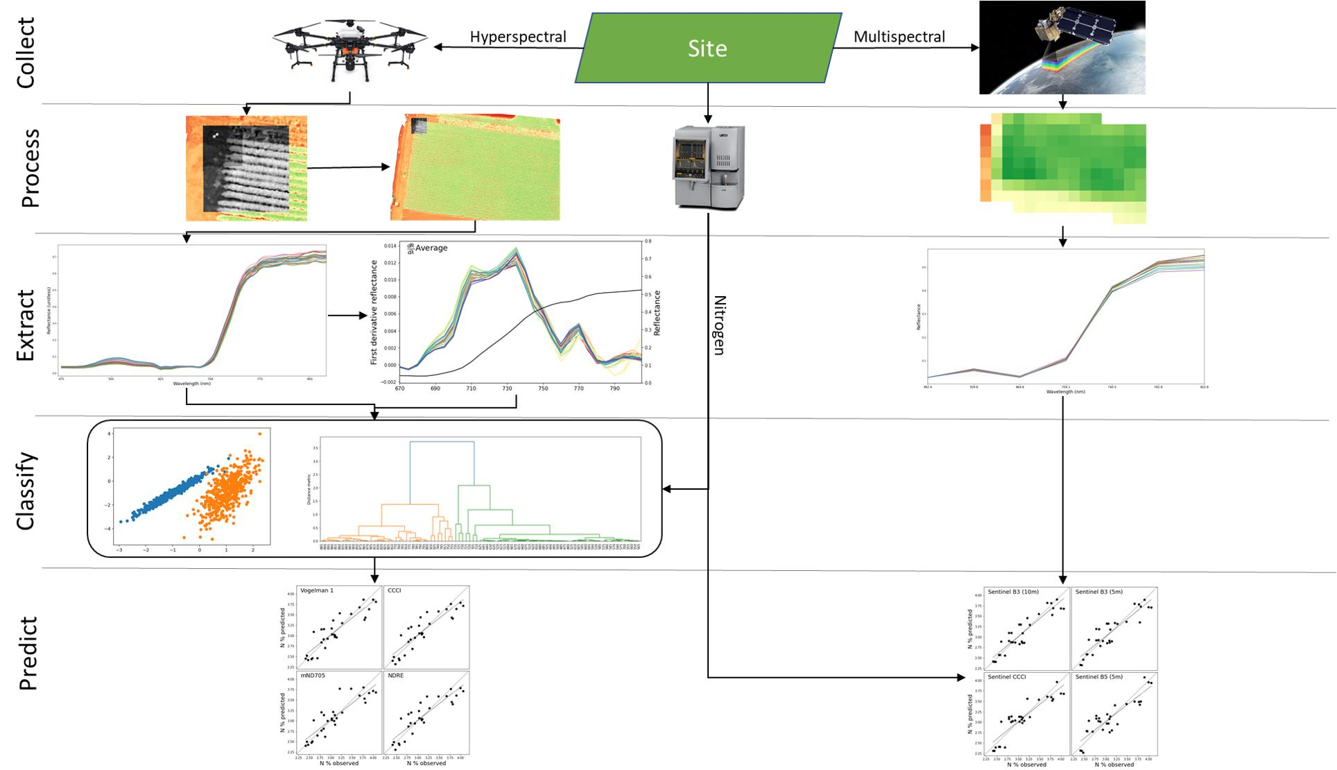
3.1. Hyperspectral Reflectance

Initial reflectance vectors from the single pixel contrasted heavily with the average areal estimate, with much greater noise from the red region onwards (Figure 2a,b). Due to the high noise and atypical reflectance curves of the single pixel vectors, the average reflectance was used throughout the analysis.

When reflectance over the red edge was separated into samples with N concentration lower or higher than 3%, there was a clear shift in the mean reflectance curve towards the NIR region for higher N levels (Figure 3a). The impact of differing N levels can also be seen in the derivative spectra, with the curve offset to longer wavelengths for higher N (Figure 3b). The field sampled N concentration was highly correlated with the N treatment applied (r = 0.87).

The first derivative curve around the red edge (Figure 4) showed a clear separation into REmin, REmid, and REmax bands, used in the calculation of the derivative VIs (e.g., NDDA). The REmid band identified from the hyperspectral derivative peaks assessment (720 nm) agreed with the iterative method of Miller, Hare, and Wu (1990), and was between the 710 nm returned by Bonham-Carter’s (1988) approach and the 730 nm derived from the slope intercept technique of Cho and Skidmore (2006).

3.2. Vegetation Indices

The VIs were mixed in their ability to predict N variability across the site (

Table 2. Vegetation Indices results.

VI	RMSE	R2	LCC	Equation
RIDAmid	0.210	0.813	0.898	y = 1.491x − 0.065
VOG1	0.214	0.806	0.894	y = 4.71x − 6.161
DIDAmid	0.222	0.791	0.885	y = 54.436x + 0.682
CCCI	0.222	0.789	0.884	y = 12.683x − 3.6
mND705	0.223	0.788	0.884	y = 15.827x − 9.577
NDDAmid	0.226	0.783	0.880	y = 7.072x + 0.598
NDRE	0.227	0.780	0.878	y = 12.856x − 2.935
RSDRmid	0.273	0.682	0.815	y = 84.685x − 4.091
LSDRmid	0.282	0.662	0.800	y = −106.438x + 7.413
$\frac{\mathrm{TCARI}}{\mathrm{OSAVI}}$	0.292	0.636	0.786	y = 1.511x + 6.171
NDVI	0.325	0.550	0.720	y = 56.311x − 46.92

* GSD: Ground Sampling Distance or spatial resolution.

). The VI which used the ratio of the area of the right side of the first derivative curve the area under the left side of the curve explained the most variation of all VIs (RIDAmid; R² = 0.813, RMSE = 0.21 and LCC = 0.898). Several other derivative-based VIs also showed good results (DIDAmid and NDDAmid providing similar results as RIDAmid), with those based on including only a single side of the derivative curve performed less well than the others (e.g., RSDRmid with R² = 0.682, RMSE = 0.273 and LCC = 0.815). Out of the traditional VIs based on nominal reflectance values, VOG1 had the best predictive ability (R² = 0.806, RMSE = 0.214 and LCC = 0.894) with CCCI, mND705, and NDRE also performing well.

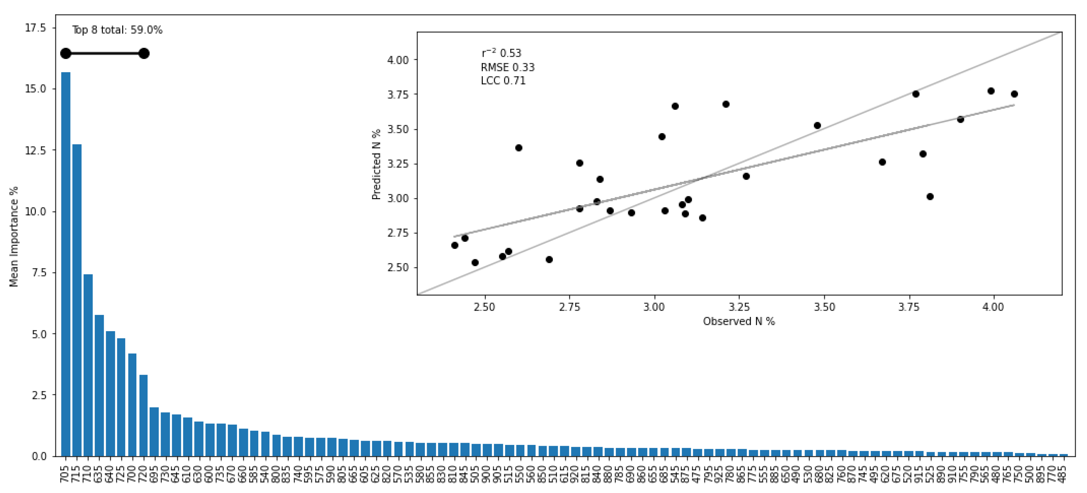
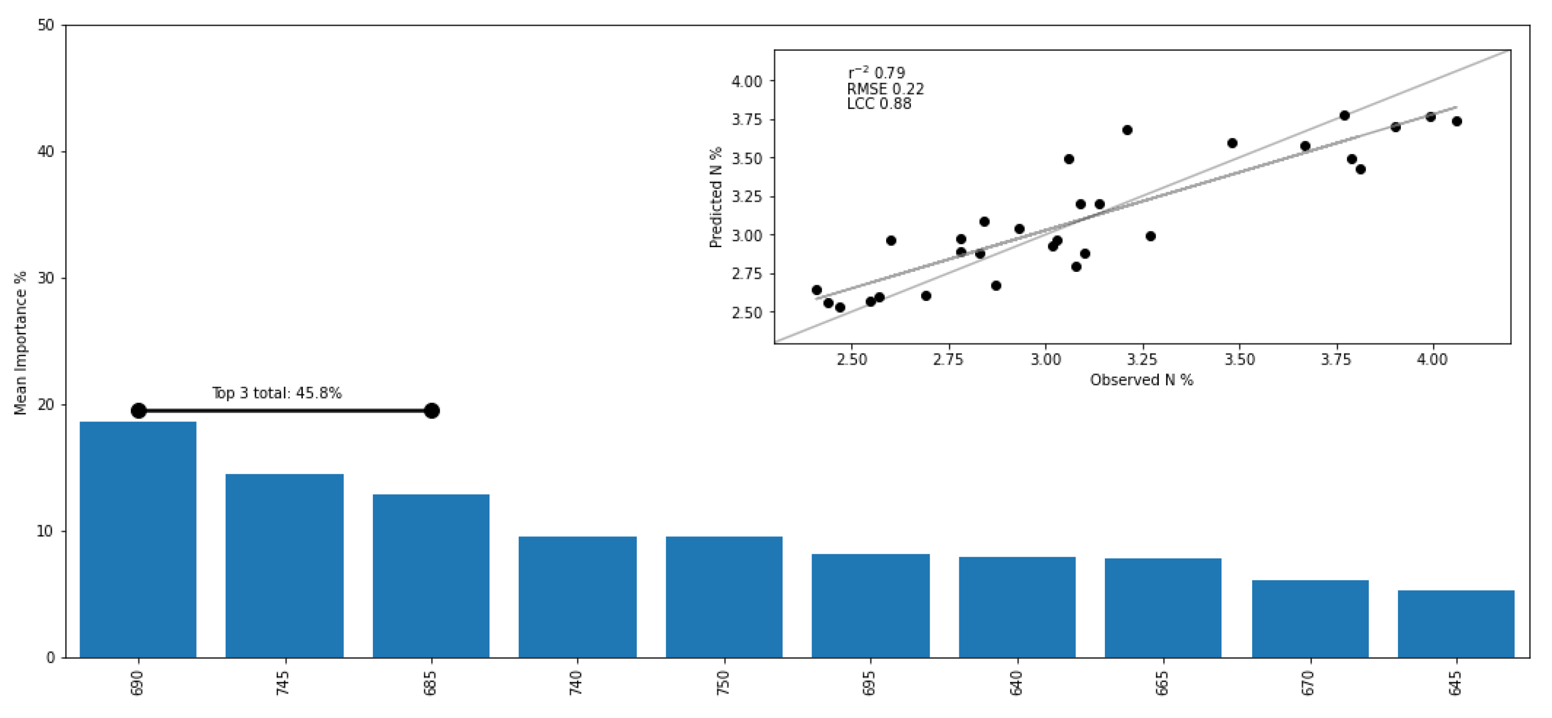
3.3. Machine Learning of Hyperspectral Reflectance for Optimised N Prediction

To explore the ability of machine learning to classify the reflectance bands into clusters based on their relationship with N concentration, density-based scanning was used after principal component analysis. The first two principal components explained 99% of the variance in the dataset. Figure 5 shows two strong clusters that were classified by the DBSCAN algorithm; one in the visible spectral region (475–715 nm separated from another in the top of the red edge and NIR (740–920 nm). The 720–735 nm and 925 nm bands were found to be noise in the clustering.

Hierarchical clustering showed the same split with bands < 740 nm in one cluster and those ≥ 740 nm in another (Figure 6). Further, the region 705–735 nm is separated in its own sub-group (labelled ‘RE’ in Figure 6). The grouping on the right side of the NIR main cluster (labelled ‘Mix’) is composed of 740–755 nm and 915–925 nm. While the ‘RE’ and ‘Mix’ regions have been clustered in separate larger hierarchies, both have similar and much larger distance metrics than either of the left and right extremes of the dendrogram (labelled ‘NIR’ and ‘RGB’ respectively).

Random forest regression over the full 91 bands returned a similar grouping (Figure 7) showing the top 20 bands were between 540 nm and 715 nm. The red edge inflection point (705–715 nm) had the best mean importance across all cross validation increments with 35.8% total. When only the top 10 most important bands were analysed using random forest, the predictive ability was near identical, with the top four bands being at the red edge inflection point 700–715 nm and accounting for over half the relative importance (Figure 8). The top 15 bands subset returned no improvement over the top 10 bands (not shown).

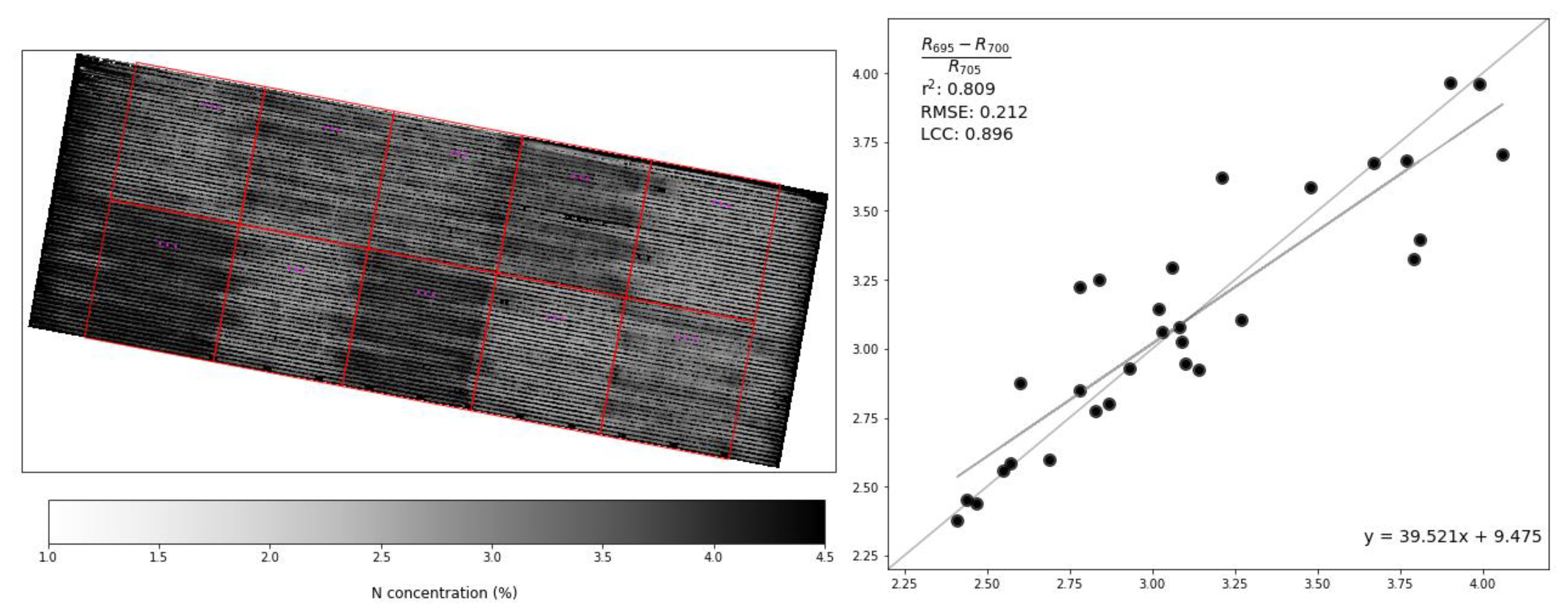
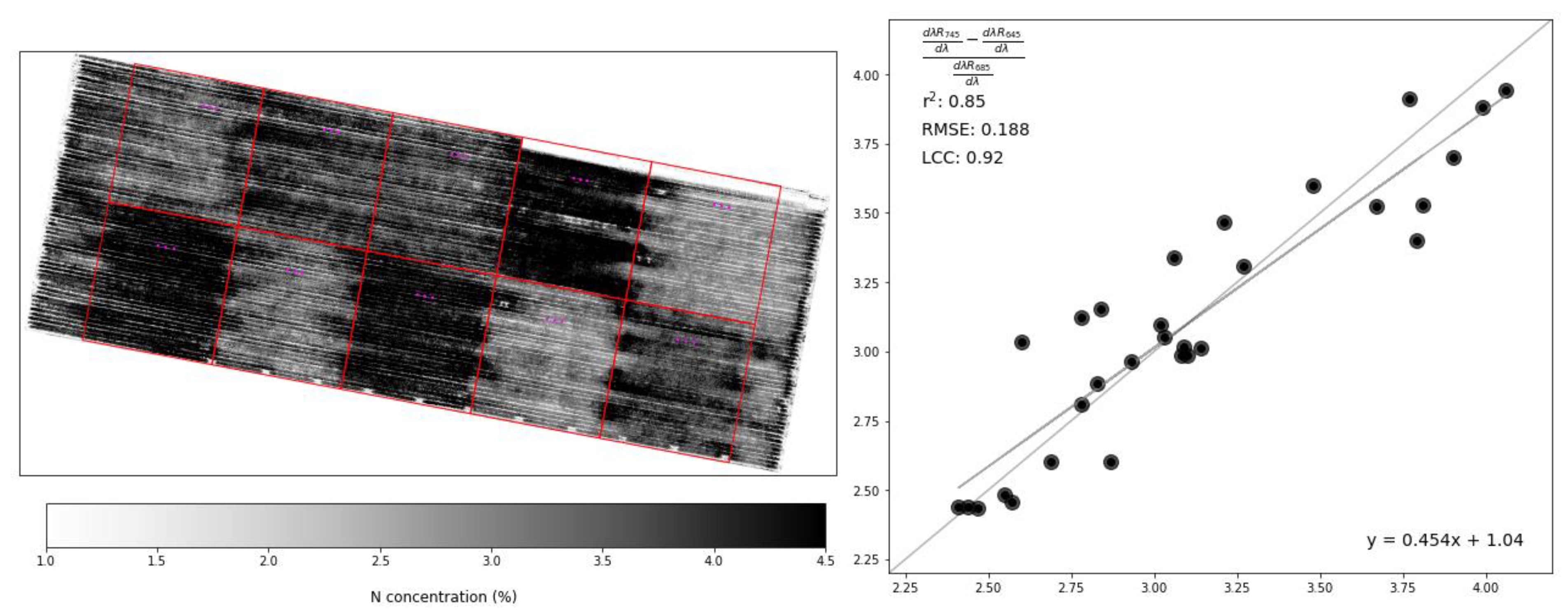
3.4. Novel Hyperspectral Vegetation Indices

All possible configurations of the top 10 bands identified by Random Forest regression were iteratively combined into three band difference, sum and product ratios. When these 2700 band combinations were tested against N, 1832 had R² > 0.40, but only 20 had R² > 0.80. The best novel VI (Figure 9) had similar or better predictive ability than most other remote sensing products tested (R² = 0.809, RMSE = 0.212 and LCC = 0.896). The exceptions being the Sentinel Green (B3) band and RIDAmid (Table 2 and

Table 3. Sentinel N prediction results.

Band	GSD (m)	RMSE	R2	LCC	Equation
Green (B3 543–578 nm)	10	0.187	0.852	0.921	y = −163.972 x + 13.22
Green (B3 543–578 nm)	5	0.204	0.823	0.904	y = −161.298x + 13.001
CCCI	5	0.208	0.816	0.900	y = 29.96x − 19.133
REP1 (B5 698–713 nm)	5	0.225	0.785	0.882	y = −114.364x + 15.364
$\frac{\mathrm{TCARI}}{\mathrm{OSAVI}}$	5	0.236	0.762	0.868	y = −44.607x + 10.538
mND705	5	0.242	0.750	0.861	y = 27.209x − 14.748
NDRE	5	0.243	0.748	0.860	y = 23.798x − 12.602
VOG1	5	0.260	0.713	0.838	y = 2.516x − 6.481
REP1 (B5 698–713 nm)	20	0.271	0.688	0.818	y = −110.096x + 14.984
NIR (B8 785–899 nm)	5	0.355	0.462	0.642	y = 19.512 − 7.12
REP3 (B7 773–793 nm)	5	0.391	0.348	0.536	y = 22.854 − 8.588
NDVI	5	0.395	0.337	0.531	y = 36.428x − 29.282
Red (B4 650–680 nm)	5	0.442	0.169	0.328	y = −152.78x + 7.798
REP2 (B6 733–748 nm)	5	0.486	0.000	0.085	y = 22.348 − 6.007
Blue (B2 458–523 nm)	5	0.488	0.000	0.064	y = −314.119x + 12.034

* GSD: Ground Sampling Distance or spatial resolution.

respectively). The novel VI focuses on the inflection point from the absorption well in the red region to the reflection peak in NIR and is referred to as the inflection point ratio vegetation index (IPRVI) and is calculated as:

$$IPRVI= \frac{\left(R_{695}- R_{700}\right)}{R_{705}}$$

(5)

where R is the reflectance at wavelength $\lambda$.

When applied to the derivative spectra, notable differences emerged from the reflectance in the bands identified in the supervised learning, with bands closer to the left and right slopes of the double peak feature being most important (685–695 nm and 740–750 nm). The regression using these 10 bands was able to explain 79% of the variation in the N samples, an improvement on the 74% when incorporating all 91 bands (Figure 10 and Figure 11).

Applying these 10 bands in the same iterative optimisation approach as for nominal reflectance, there were 1,424 combinations which had R² > 0.40, while 286 had R² > 0.80. The best novel derivative VI (Figure 12) had a similar result as the Sentinel Green band, while giving a stronger separation between the treatment plots in the novel reflectance VI. The derivative inflection point ratio vegetation index (DIPRVI) leverages information from a broader spectral window to characterise the transition from green into red and red-edge into NIR regions, scaled by the trough of the red absorption well, and is calculated as:

$$DIPRVI= \frac{\frac{d\lambda R_{745}}{d\lambda }- \frac{d\lambda R_{645}}{d\lambda }}{\frac{d\lambda R_{685}}{d\lambda }}$$

(6)

where $\frac{d\lambda R}{d\lambda }$ is the first order reflectance derivative at wavelength $\lambda$.

The application of the iteratively identified linear equation to the derivative spectra did show some instability in the tractor rows and near the stitching artefact along the top row on the right side of the array.

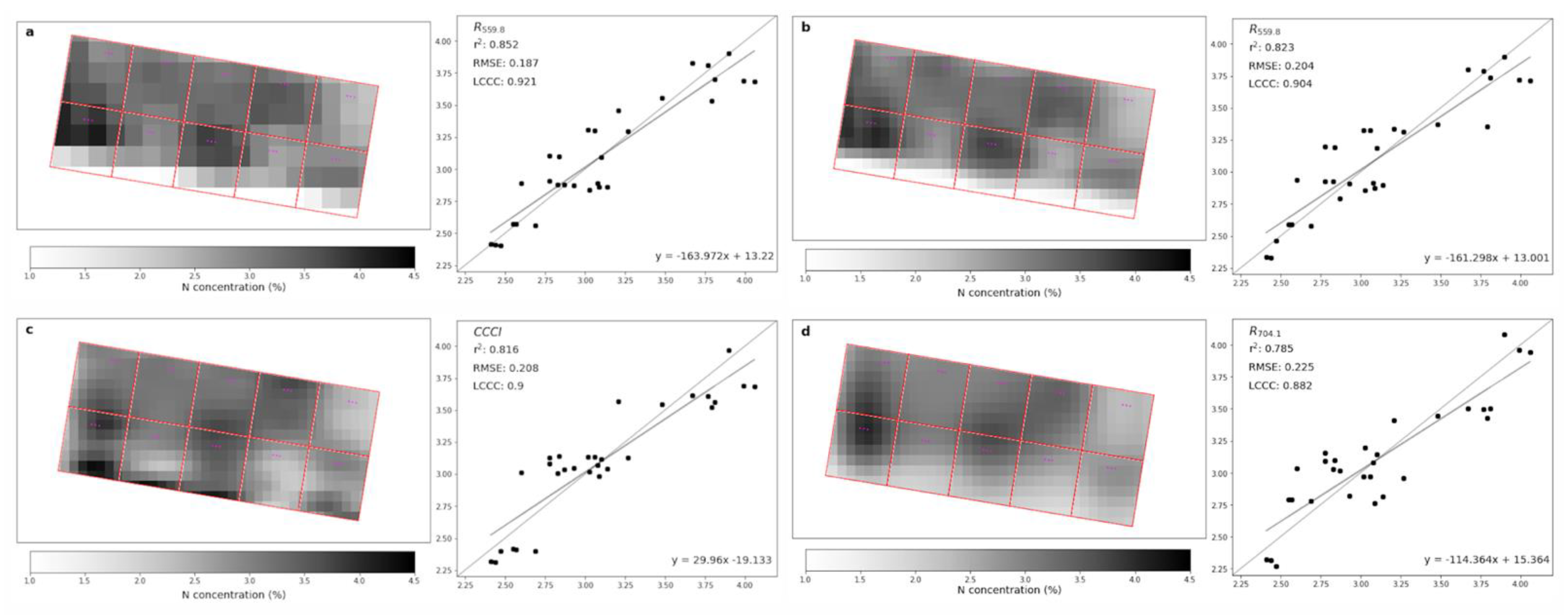
3.5. Sentinel Reflectance

Sampled reflectance from the Sentinel bands had mixed performance in predicting N (Table 3; best 4 N predictions in Figure 13a–d). Out of the raw bands, Sentinel bands 3 and 5 each explained most of the variation in the N samples across the trial site, with the 10 m Green (B3) outperforming the Green at 5 m and all others. The VIs calculated from the Sentinel layers had a similar performance in predicting N to those derived from the hyperspectral data, with CCCI the best at predicting N with a slightly improved R² (0.81 vs. 0.78) while $\frac{\mathrm{TCARI}}{\mathrm{OSAVI}}$ was materially improved with R² rising from 0.63 to 0.76. The two top performing hyperspectral VIs VOG1 and mND705 were much less effective in predicting N when calculated using the Sentinel layers, with VOG1 R² dropping from 0.81 to 0.71). The Red Edge Point 1 band (B5) had a strong performance when downscaled to 5 m, but less so at its native 20 m resolution. The hyperspectral imagery was binned to match the discrete sentinel spectral ranges and tested, with the averaged hyperspectral bands matching the sentinel Red Edge Point 1 performing better than the Green region at predicting N concentration (R² of 0.672, RMSE of 0.277, LCC of 0.807 and R² of 0.433, RMSE of 0.364 LCC of 0.62, respectively).

4. Discussion

4.1. Hyperspectral Performance

The hyperspectral imagery had very high spatial resolution (~5.2 cm) giving the ability to discriminate individual plant crowns, crop rows and field features such as low vigour areas on the edges, as well as gaps in canopy cover. Comparing Figure 1,Figure 9 and Figure 12, the treatment plots and buffer regions are clearly visible, with the different areas within treatment plots that responded strongly to the applied N distinguishable with those that may require further investigation for subsoil or other constraints. The ability to identify inter-plot as well as intra-plot variability provides insight for the implementation of precision agriculture approaches. These results suggest that high resolution hyperspectral remote sensing would be able to detect fine-scale variability, allowing more tailored management in a broadacre cropping commercial setting.

The average areal reflectance (Figure 2a) had a stronger relationship with N concentration than the single pixel values (Figure 2b) and so average areal reflectance was used throughout this study. This is most likely due to three main causes: (1) the mature canopy structure of the cotton stands had multiple layers of leaves returning additive transmittance and reflectance that could distort the signal received at the sensor; (2) impact of Bi-directional Reflectance Distribution Function from the highly variable geometry of individual leaves relative to the sensor pixel’s individual field of view; and, (3) the field N samples were areal averages taken from multiple plants around a location so an averaged signal represents the N impact on canopy reflectance more accurately. Upscaling from leaf level to canopy reflectance has been found to introduce strong spectral noise from including green along with non-green elements and canopy structure [10].

Interestingly, the simpler remote sensing approaches gave some of the strongest predictions of N across the trial site. Indices such as TVI or TCARI-OSAVI are robust against soil background, for this experiment, however, the reflectance vectors were sampled from the middle of the crop rows and had minimal to no impact from soil reflectance. The indices that included fewer bands focussing on photosynthetically active spectral regions were more successful in detecting N than those which included additional bands to reduce the impact of confounding factors. As expected with a mature closed canopy, NDVI performed poorly most likely due to the high LAI causing saturation, whereas NDRE and the red edge VIs performed strongly, the red edge being less affected by the spongy mesophyll layers in plant leaves than NIR.

The critical role of the red edge spectral region is clearly demonstrated by the performance of both the simple (VOG1, NDRE and mND705) and derivative spectra VIs (RIDAmid, DIDAmid, and NDDAmid). The supervised and unsupervised learning results from the hyperspectral dataset shown in the novel IPRVI from this study confirmed the importance of the red edge inflection point around 705 nm to reflectance samples. Similarly, the shape of the curve between the red and red edge regions (the 645 nm, 685 nm and 745 nm) was more critical to derivative spectra and the novel DIPRVI discussed in this study. As seen in Figure 3a, the mean reflectance curve for the group of samples with higher apparent N is shifted to longer wavelengths on the right, and in Figure 3b the importance of spectra around the slope of the peak shows the separation between N levels clearly with the slope being around 5 nm shorter in wavelength on each of the peak’s sides for the lower N levels. Those derivative spectra VIs which incorporated both sides of the peak performed better than single side area indices as the full range of spectral information available in the red edge region, both the inflection points near red (left side) and NIR (right side), provided better distinction between plants with lower N reflecting more energy as higher N plants continued absorbing.

The novel VI results use these key bands identified in the machine learning to maximise the information content in this spectral region. The reflectance VI focuses solely on the inflection point, while the derivative VI leverages the gradient and position of the peak’s sides. There is a useful comparison in the performance of the two iterative regression results. While the nominal reflectance returned more ratios with moderate predictive ability than the derivative spectra (1832 and 1424 with R² > 0.40 respectively), while having fewer ratios with high predictive potential (20 and 286 with R² > 0.80 respectively). This suggests the information content for predicting N concentration in the derivative spectra is worth further investigation. With the higher N content due to applied N, leaves are able to sustain greater chlorophyll pigment levels and so absorb more radiation for photosynthesis, leading to the wider red region absorption well and the red edge shift into longer wavelengths. With the crop being irrigated the possibility of highly variable water content levels between plants is reduced. A small gradient in plant water availability due to minor differences in soil type or other factors may be responsible for the limited variability visible within the treatment zones in the hyperspectral data.

4.2. Machine Learning Impact

The machine learning approach narrowed the range of bands required to investigate plant condition over this trial site, greatly improved processing time and reduced processing complexity. Iterative optimisation over the machine learning identified subset of 10 bands compared to the full 91 bands in the hyperspectral datacube, sped up processing dramatically. Even with parallel processing, testing the full datacube took more than 8 h, as opposed to ~40 min for the subset. Further, the approach of using clustering along with multilayered decision trees is useful to explore the spectral feature space from different approaches as evidence for band selection. This approach may be useful to explore labelled training data of other variables of interest.

When implementing extreme boosted gradient trees, however, the result was discarded as the “F-score” metric, basically an indicator of frequency of splits on the variable, returned the first band as the most important by a factor of more than 3 for both single and average pixels as well as derivative spectra (not shown). Partial least squares regression returned similar results to the random forest investigation (not shown). Machine learning promises useful classification and prediction potential, however, with the more sophisticated approaches, there is considerable complexity. This can involve substantial pre-processing, which can have non-trivial impacts on both multispectral and hyperspectral imagery, as, for example, both have large null value regions around the borders.

4.3. Sentinel Performance

The Sentinel Green B3 product at 10 m ground sampling distance performed the best out of the imagery tested on this sample set, with slightly lower error compared to the best derivative spectra VI (RMSE = 0.187 vs. 0.188). The performance of the red edge B5 product at 5 m was similar to many of the conventional VIs, however, lower than expected considering the results from the other red edge VIs and machine learning tests. At native 20 m resolution it was amongst the lowest prediction outcomes. While the 550 nm band is important for photosynthesis, its relatively higher reflectance and smaller variation across the reflectance samples (Sentinel reflectance curve is very similar in outline to Figure 3b) most likely reduced its importance in the hyperspectral analysis of the present study. Out of the Sentinel VIs, the performance was very similar to the hyperspectral VIs, though with VOG1 and mND705 performing less well. VOG1 may have been impacted by a poor fit of the Sentinel bands to its prescribed configuration, as there is no Sentinel band that easily fits the VI’s denominator (720 nm). For this study, we used $\frac{REP2}{REP1}$, though REP1 ends at approximately 713 nm. CCCI having a strong prediction ability is not surprising generally as it was conceived to represent chlorophyll content, which is strongly correlated with N concentration in crop canopies and performed very similarly to its hyperspectral counterpart.

The positions of the samples relative to the pixel boundaries may have influenced the stronger performance of some Sentinel bands over other remote sensing data used in this study. For example, at the south edge of the Sentinel arrays (Figure 13a–d) the impact of the empty paddock on that side is evident in N concentration predictions of ~1%. This may lie behind the relatively poorer red edge performance. When this was tested by replicating the spectral ranges of the sentinel instrument with the hyperspectral dataset the predictive ability dropped dramatically for the B3 equivalent spectral range, while those approximating the B5 band showed much reduced predictive ability. This suggests the strong performance of the Sentinel B3 band on these samples is more likely due to the pixel position relative to the sample position, rather than the strength of the spectral information itself. The mixed pixel effects of having multiple alternating crop canopy and tractor rows combined, even at 5 m GSD would also impact bands in different ways; for example, the moderate reflectance of the green bands may be less impacted than the higher reflectance red edge. Additionally, with the study site being well-irrigated, the impact of wet soil, which has a similar reflectance to vegetation at 550 nm, may homogenise the signal received by the Sentinel MSI, whereas all other bands would be more heavily impacted by variability in spectral response within the mixed pixel.

For broadacre crop scale applications where a pixel size of 20 m is ample discrimination and pixel boundaries are less relevant, Sentinel products provide a low-cost data source with a long historical record to inform precision agriculture and site management. For a research context, however, many field plots are significantly smaller than 10 m on all sides and Sentinel data may not be suitable. The overflight schedule can also pose a challenge to match data collection to key phenology milestones.

5. Conclusions

The main objectives of this study were to explore machine learning of a hyperspectral datacube to identify novel reflectance measures of cotton canopy nitrogen concentration and compare UAV hyperspectral against satellite multispectral remote sensing. There were several key outcomes:

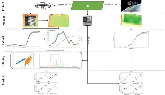
• The hyperspectral datacube reported in this study was able to predict N levels across the site with high accuracy, both from simpler conventional VIs as well as machine learning derived VIs. The crop features were clearly discernible at plot, row, and down to plant scale.
• A machine learning approach narrows the optimisation search window making new spectral features easier and quicker to find and test.
• Sentinel data proved capable with these field samples to delineate N levels at coarse, production scale, though the sample locations compared to pixel boundaries suggest further comparison is needed.
• There were challenges with this study that could be addressed with further research. While the stitching artefacts had no impact on the sampled reflectance due to the field sample location being distant from the area involved, the stitching does impact the ability to visually infer N levels from that part of the field.
• The high-resolution continuous spectra argue for hyperspectral remote sensing’s ability to identify inter-plot as well as intra-plot variability, providing strong insight for development and refinement of a precision agriculture strategy while UAV platforms demonstrate high spatial resolution and responsiveness to producers or researchers needs. The machine learning derived VIs need further testing to ensure this performance holds across multiple seasons, sites and crops.

References

1. Raper, T.B.; Varco, J.J. Canopy-scale wavelength and vegetative index sensitivities to cotton growth parameters and nitrogen status. Precis. Agric. 2014, 16, 62–76. [Google Scholar] [CrossRef] [Green Version]
2. Rosolem, C.; Mikkelsen, D. Nitrogen source-sink relationship in cotton. J. Plant Nutr. 1989, 12, 1417–1433. [Google Scholar] [CrossRef]
3. Yang, G.; Tang, H.; Nie, Y.; Zhang, X. Responses of cotton growth, yield, and biomass to nitrogen split application ratio. Eur. J. Agron. 2011, 35, 164–170. [Google Scholar] [CrossRef]
4. Chen, J.; Liu, L.; Wang, Z.; Sun, H.; Zhang, Y.; Bai, Z.; Song, S.; Lu, Z.; Li, C. Nitrogen Fertilization Effects on Physiology of the Cotton Boll–Leaf System. Agronomy 2019, 9, 271. [Google Scholar] [CrossRef] [Green Version]
5. Diaz, R.J.; Rosenberg, R. Spreading Dead Zones and Consequences for Marine Ecosystems. Science 2008, 321, 926–929. [Google Scholar] [CrossRef] [PubMed]
6. Padilla, F.M.; Gallardo, M.; Manzano-Agugliaro, F. Global trends in nitrate leaching research in the 1960–2017 period. Sci. Total Environ. 2018, 643, 400–413. [Google Scholar] [CrossRef]
7. Blesh, J.; Drinkwater, L.E. The impact of nitrogen source and crop rotation on nitrogen mass balances in the Mississippi River Basin. Ecol. Appl. 2013, 23, 1017–1035. [Google Scholar] [CrossRef]
8. Macdonald, B.C.T.; Latimer, J.O.; Schwenke, G.D.; Nachimuthu, G.; Baird, J.C. The current status of nitrogen fertiliser use efficiency and future research directions for the Australian cotton industry. J. Cotton Res. 2018, 1, 15. [Google Scholar] [CrossRef]
9. Ju, C.-H.; Tian, Y.-C.; Yao, X.; Cao, W.-X.; Zhu, Y.; Hannaway, D. Estimating Leaf Chlorophyll Content Using Red Edge Parameters. Pedosphere 2010, 20, 633–644. [Google Scholar] [CrossRef]
10. Main, R.; Cho, M.A.; Mathieu, R.; O’Kennedy, M.M.; Ramoelo, A.; Koch, S. An investigation into robust spectral indices for leaf chlorophyll estimation. ISPRS J. Photogramm. Remote Sens. 2011, 66, 751–761. [Google Scholar] [CrossRef]
11. Dorigo, W.A.; Zurita-Milla, R.; De Wit, A.J.W.; Brazile, J.; Singh, R.; Schaepman, M.E. A review on reflective remote sensing and data assimilation techniques for enhanced agroecosystem modeling. Int. J. Appl. Earth Obs. Geoinf. 2007, 9, 165–193. [Google Scholar] [CrossRef]
12. Cho, M.A.; Skidmore, A.K. A new technique for extracting the red edge position from hyperspectral data: The linear extrapolation method. Remote Sens. Environ. 2006, 101, 181–193. [Google Scholar] [CrossRef]
13. Feng, W.; Guo, B.-B.; Wang, Z.-J.; He, L.; Song, X.; Wang, Y.-H.; Guo, T.-C. Measuring leaf nitrogen concentration in winter wheat using double-peak spectral reflection remote sensing data. Field Crop. Res. 2014, 159, 43–52. [Google Scholar] [CrossRef]
14. Horler, D.N.H.; Dockray, M.; Barber, J. The red edge of plant leaf reflectance. Int. J. Remote Sens. 1983, 4, 273–288. [Google Scholar] [CrossRef]
15. Broge, N.H.; Leblanc, E. Comparing prediction power and stability of broadband and hyperspectral vegetation indices for estimation of green leaf area index and canopy chlorophyll density. Remote Sens. Environ. 2001, 76, 156–172. [Google Scholar] [CrossRef]
16. Boochs, F.; Kupfer, G.; Dockter, K.; Kühbauch, W. Shape of the red edge as vitality indicator for plants. Int. J. Remote Sens. 1990, 11, 1741–1753. [Google Scholar] [CrossRef]
17. Frazier, A.E.; Wang, L.; Chen, J. Two new hyperspectral indices for comparing vegetation chlorophyll content. Geo-Spat. Inf. Sci. 2014, 17, 17–25. [Google Scholar] [CrossRef]
18. García-Berná, J.A.; Ouhbi, S.; Benmouna, B.; García-Mateos, G.; Fernández-Alemán, J.L.; Molina-Martínez, J.M. Systematic mapping study on remote sensing in agriculture. Appl. Sci. 2020, 10, 3456. [Google Scholar] [CrossRef]
19. Sims, D.A.; Gamon, J.A. Relationships between leaf pigment content and spectral reflectance across a wide range of species, leaf structures and developmental stages. Remote Sens. Environ. 2002, 81, 337–354. [Google Scholar] [CrossRef]
20. Nicodemus, F.E. Earrtum: Directional Reflectance and Emissivity of an Opaque Surface. Appl. Opt. 1966, 5, 715. [Google Scholar] [CrossRef]
21. Jensen, J.R. Remote Sensing of the Environment: An Earth Resource Perspective; Prentice Hall: Upper Saddle River, NJ, USA, 2000. [Google Scholar]
22. Weiss, M.; Jacob, F.; Duveiller, G. Remote sensing for agricultural applications: A meta-review. Remote Sens. Environ. 2020, 236, 111402. [Google Scholar] [CrossRef]
23. Aasen, H.; Bolten, A. Multi-temporal high-resolution imaging spectroscopy with hyperspectral 2D imagers—From theory to application. Remote Sens. Environ. 2018, 205, 374–389. [Google Scholar] [CrossRef]
24. Boggs, J.L.; Tsegaye, T.D.; Coleman, T.L.; Reddy, K.C.; Fahsi, A. Relationship between Hyperspectral Reflectance, Soil Nitrate-Nitrogen, Cotton Leaf Chlorophyll, and Cotton Yield: A Step toward Precision Agriculture. J. Sustain. Agric. 2003, 22, 5–16. [Google Scholar] [CrossRef]
25. Zhao, D.; Reddy, K.R.; Kakani, V.G.; Read, J.J.; Koti, S. Selection of Optimum Reflectance Ratios for Estimating Leaf Nitrogen and Chlorophyll Concentrations of Field-Grown Cotton. Agron. J. 2005, 97, 89–98. [Google Scholar] [CrossRef] [Green Version]
26. Buscaglia, H.J.; Varco, J.J. Early Detection of Cotton Leaf Nitrogen Status Using Leaf Reflectance. J. Plant Nutr. 2002, 25, 2067. [Google Scholar] [CrossRef]
27. Hunt, R.E., Jr.; Cavigelli, M.; Daughtry, C.S.T.; McMurtrey, J.E.; Walthall, C.L. Evaluation of Digital Photography from Model Aircraft for Remote Sensing of Crop Biomass and Nitrogen Status. Precis. Agric. 2005, 6, 359–378. [Google Scholar] [CrossRef]
28. Tarpley, L.; Reddy, K.R.; Sassenrath-Cole, G.F. Reflectance indices with precision and accuracy in predicting cotton leaf nitrogen concentration. Crop. Sci. 2000, 40, 1814–1819. [Google Scholar] [CrossRef]
29. Feng, A.; Zhou, J.; Vories, E.; Sudduth, K.A. Evaluation of cotton emergence using UAV-based imagery and deep learning. Comput. Electron. Agric. 2020, 177, 105711. [Google Scholar] [CrossRef]
30. Chen, R.; Chu, T.; Landivar, J.A.; Yang, C.; Maeda, M.M. Monitoring cotton (Gossypium hirsutum L.) germination using ultrahigh-resolution UAS images. Precis. Agric. 2018, 19, 161–177. [Google Scholar] [CrossRef]
31. Yang, C.; Everitt, J.H.; Bradford, J.M.; Murden, D. Airborne Hyperspectral Imagery and Yield Monitor Data for Mapping Cotton Yield Variability. Precis. Agric. 2004, 5, 445–461. [Google Scholar] [CrossRef]
32. Filippi, P.; Whelan, B.M.; Vervoort, R.W.; Bishop, T.F. Mid-season empirical cotton yield forecasts at fine resolutions using large yield mapping datasets and diverse spatial covariates. Agric. Syst. 2020, 184, 102894. [Google Scholar] [CrossRef]
33. Reisig, D.D.; Godfrey, L.D. Remotely Sensing Arthropod and Nutrient Stressed Plants: A Case Study With Nitrogen and Cotton Aphid (Hemiptera: Aphididae). Environ. Entomol. 2010, 39, 1255–1263. [Google Scholar] [CrossRef] [Green Version]
34. Lowe, A.; Harrison, N.; French, A.P. Hyperspectral image analysis techniques for the detection and classification of the early onset of plant disease and stress. Plant Methods 2017, 13, 1–12. [Google Scholar] [CrossRef]
35. Zhu, L.; Suomalainen, J.; Liu, J.; Hyyppä, J.; Kaartinen, H.; Haggren, H. A Review: Remote Sensing Sensors. Multi-Purp. Appl. Geospat. Data 2018. [Google Scholar] [CrossRef] [Green Version]
36. Rouse, J.W. Monitoring the Vernal Advancement and Retrogradation (Green Wave Effect) of Natural Vegetation; SienceOpen: Burlington, MA, USA, 1973. [Google Scholar]
37. Gitelson, A.A.; Merzlyak, M.N. Remote estimation of chlorophyll content in higher plant leaves. Int. J. Remote Sens. 1997, 18, 2691–2697. [Google Scholar] [CrossRef]
38. Vogelmann, J.E.; Rock, B.N.; Moss, D.M. Red edge spectral measurements from sugar maple leaves. Int. J. Remote Sens. 1993, 14, 1563–1575. [Google Scholar] [CrossRef]
39. Barnes, E.M.; Clarke, T.R.; Richards, S.E.; Colaizzi, P.D.; Haberland, J.; Kostrzewski, M.; Waller, P.; Choi, C.; Riley, E.; Thompson, T.; et al. Coincident detection of crop water stress, nitrogen status and canopy density using ground based multispectral data. In Proceedings of the Fifth International Conference on Precision Agriculture, Bloomington, MN, USA, 16–19 July 2000. [Google Scholar]
40. Haboudane, D.; Miller, J.R.; Tremblay, N.; Zarco-Tejada, P.J.; Dextraze, L. Integrated narrow-band vegetation indices for prediction of crop chlorophyll content for application to precision agriculture. Remote Sens. Environ. 2002, 81, 416–426. [Google Scholar] [CrossRef]
41. Fridgen, J.L.; Varco, J.J. Dependency of Cotton Leaf Nitrogen, Chlorophyll, and Reflectance on Nitrogen and Potassium Availability. Agron. J. 2004, 96, 63–69. [Google Scholar] [CrossRef]
42. Le Maire, G.; François, C.; Dufrêne, E. Towards universal broad leaf chlorophyll indices using PROSPECT simulated database and hyperspectral reflectance measurements. Remote Sens. Environ. 2004, 89, 1–28. [Google Scholar] [CrossRef]
43. Miller, J.R.; Hare, E.W.; Wu, J. Quantitative characterization of the vegetation red edge reflectance an inverted-Gaussian reflectance model. Int. J. Remote Sens. 1990, 11, 1755–1773. [Google Scholar] [CrossRef]
44. Bonham-Carter, G. Numerical procedures and computer program for fitting an inverted gaussian model to vegetation reflectance data. Comput. Geosci. 1988, 14, 339–356. [Google Scholar] [CrossRef]
45. Kochubey, S.M.; Kazantsev, T.A. Derivative vegetation indices as a new approach in remote sensing of vegetation. Front. Earth Sci. 2012, 6, 188–195. [Google Scholar] [CrossRef]
46. Drusch, M.; Del Bello, U.; Carlier, S.; Colin, O.; Fernandez, V.; Gascon, F.; Hoersch, B.; Isola, C.; Laberinti, P.; Martimort, P.; et al. Sentinel-2: ESA’s Optical High-Resolution Mission for GMES Operational Services. Remote Sens. Environ. 2012, 120, 25–36. [Google Scholar] [CrossRef]
47. Söderström, M.; Piikki, K.; Stenberg, M.; Stadig, H.; Martinsson, J. Producing nitrogen (N) uptake maps in winter wheat by combining proximal crop measurements with Sentinel-2 and DMC satellite images in a decision support system for farmers. Acta Agric. Scand. Sect. B 2017, 67, 637–650. [Google Scholar] [CrossRef]
48. Laurent, V.C.; Schaepman, M.E.; Verhoef, W.; Weyermann, J.; Chávez, R.O. Bayesian object-based estimation of LAI and chlorophyll from a simulated Sentinel-2 top-of-atmosphere radiance image. Remote Sens. Environ. 2014, 140, 318–329. [Google Scholar] [CrossRef]
49. Verrelst, J.; Camps-Valls, G.; Muñoz-Marí, J.; Rivera, J.P.; Veroustraete, F.; Clevers, J.G.; Moreno, J. Optical remote sensing and the retrieval of terrestrial vegetation bio-geophysical properties—A review. ISPRS J. Photogramm. Remote Sens. 2015, 108, 273–290. [Google Scholar] [CrossRef]
50. Rivera, J.P.; Verrelst, J.; Leonenko, G.; Moreno, J. Multiple Cost Functions and Regularization Options for Improved Retrieval of Leaf Chlorophyll Content and LAI through Inversion of the PROSAIL Model. Remote Sens. 2013, 5, 3280–3304. [Google Scholar] [CrossRef] [Green Version]
51. Habyarimana, E.; Piccard, I.; Catellani, M.; De Franceschi, P.; Dall’Agata, M. Towards Predictive Modeling of Sorghum Biomass Yields Using Fraction of Absorbed Photosynthetically Active Radiation Derived from Sentinel-2 Satellite Imagery and Supervised Machine Learning Techniques. Agronomy 2019, 9, 203. [Google Scholar] [CrossRef] [Green Version]
52. Song, Y.; Wang, J. Mapping Winter Wheat Planting Area and Monitoring Its Phenology Using Sentinel-1 Backscatter Time Series. Remote Sens. 2019, 11, 449. [Google Scholar] [CrossRef] [Green Version]
53. Meier, J.; Mauser, W.; Hank, T.; Bach, H. Assessments on the impact of high-resolution-sensor pixel sizes for common agricultural policy and smart farming services in European regions. Comput. Electron. Agric. 2020, 169, 105205. [Google Scholar] [CrossRef]
54. Bishop, C.M. Pattern Recognition and Machine Learning; Springer: New York, NY, USA, 2006. [Google Scholar]
55. Yamaguchi, T.; Tanaka, Y.; Imachi, Y.; Yamashita, M.; Katsura, K. Feasibility of Combining Deep Learning and RGB Images Obtained by Unmanned Aerial Vehicle for Leaf Area Index Estimation in Rice. Remote Sens. 2020, 13, 84. [Google Scholar] [CrossRef]
56. Zhao, W.; Yamada, W.; Li, T.; Digman, M.; Runge, T. Augmenting Crop Detection for Precision Agriculture with Deep Visual Transfer Learning—A Case Study of Bale Detection. Remote Sens. 2020, 13, 23. [Google Scholar] [CrossRef]
57. Nevavuori, P.; Narra, N.; Linna, P.; Lipping, T. Crop Yield Prediction Using Multitemporal UAV Data and Spatio-Temporal Deep Learning Models. Remote Sens. 2020, 12, 4000. [Google Scholar] [CrossRef]
58. Féret, J.-B.; le Maire, G.; Jay, S.; Berveiller, D.; Bendoula, R.; Hmimina, G.; Cheraiet, A.; Oliveira, J.; Ponzoni, F.; Solanki, T.; et al. Estimating leaf mass per area and equivalent water thickness based on leaf optical properties: Potential and limitations of physical modeling and machine learning. Remote Sens. Environ. 2019, 231, 110959. [Google Scholar] [CrossRef]
59. Hulugalle, N.R.; Weaver, T.B.; Finlay, L.A.; Lonergan, P. Soil properties, black root-rot incidence, yield, and greenhouse gas emissions in irrigated cotton cropping systems sown in a Vertosol with subsoil sodicity. Soil Res. 2012, 50, 278–292. [Google Scholar] [CrossRef]
60. Savitzky, A.; Golay, M.J.E. Smoothing and Differentiation of Data by Simplified Least Squares Procedures. Anal. Chem. 1964, 36, 1627–1639. [Google Scholar] [CrossRef]
61. Louhichi, S.; Gzara, M.; Ben Abdallah, H. A density based algorithm for discovering clusters with varied density. In Proceedings of the 2014 World Congress on Computer Applications and Information Systems (WCCAIS), Hammamet, Tunisia, 17–19 January 2014; pp. 1–6. [Google Scholar]
62. Rokach, L. A survey of Clustering Algorithms. In Data Mining and Knowledge Discovery Handbook; Springer International Publishing: Berlin/Heidelberg, Germany, 2009; pp. 269–298. [Google Scholar]
63. Gorelick, N.; Hancher, M.; Dixon, M.; Ilyushchenko, S.; Thau, D.; Moore, R. Google Earth Engine: Planetary-scale geospatial analysis for everyone. Remote Sens. Environ. 2017, 202, 18–27. [Google Scholar] [CrossRef]
Figure 1. Experimental site, Narrabri, New South Wales, Australia. Zoomed-in window shows site layout with N treatments and sample points.
Remotesensing 13 01428 g001
Figure 2. Hyperspectral reflectance at each georeferenced sample point, (a) from a single pixel, (b) from average of pixels within 20 cm.
Remotesensing 13 01428 g002
Figure 3. (a) mean spectral reflectance (b) mean derivatives in the red edge region for lower versus higher N plots.
Remotesensing 13 01428 g003
Figure 4. First derivative curve showing band separators.
Remotesensing 13 01428 g004
Figure 5. Density based scan for clustering nominal reflectance.
Remotesensing 13 01428 g005
Figure 6. Hierarchical clustering of nominal reflectance.
Remotesensing 13 01428 g006
Figure 7. Random forest regression for all reflectance bands.
Remotesensing 13 01428 g007
Figure 8. Random forest regression using only the top 10 reflectance bands.
Remotesensing 13 01428 g008
Figure 9. Novel red edge IPRVI predictions of N concentration.
Remotesensing 13 01428 g009
Figure 10. Random forest regression with derivative spectra.
Remotesensing 13 01428 g010
Figure 11. Random forest regression with top 10 derivative spectra bands.
Remotesensing 13 01428 g011
Figure 12. Novel derivative spectra VI N prediction map.
Remotesensing 13 01428 g012
Figure 13. Sentinel N prediction, (a) Green 10 m, (b) Green 5 m, (c) Sentinel CCCI 5 m, and (d) REP1 5 m GSD.
Remotesensing 13 01428 g013