
Evaluation of P-Band SAR Tomography for Mapping Tropical Forest Vertical Backscatter and Tree Height

 , and
, and
Abstract
:
1. Introduction
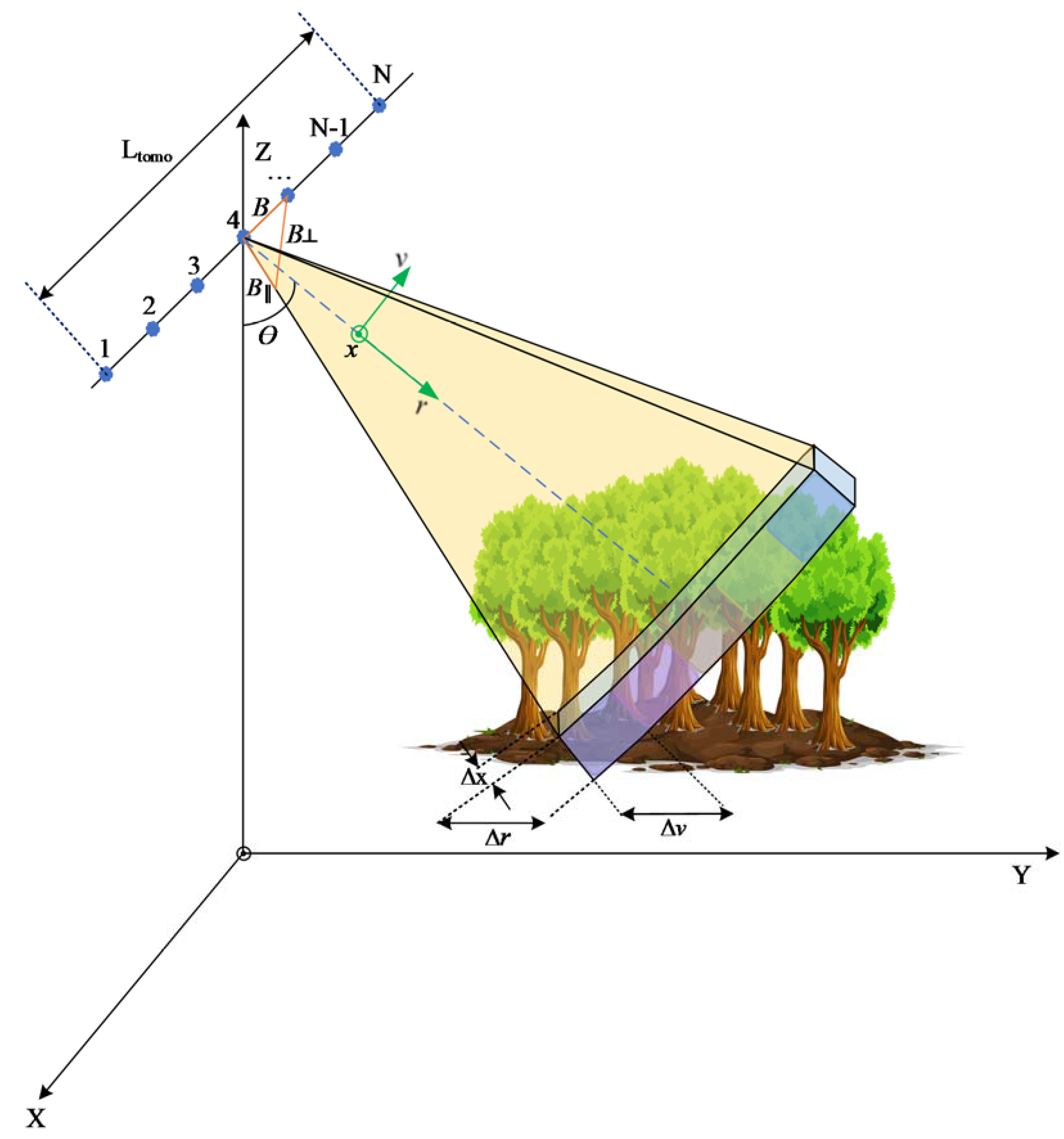
2. SAR Tomography
2.1. Signal Model and Inversion Approaches
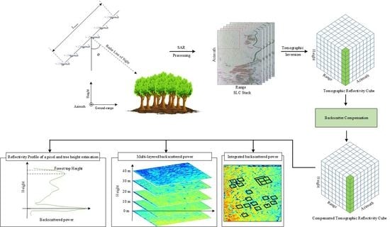
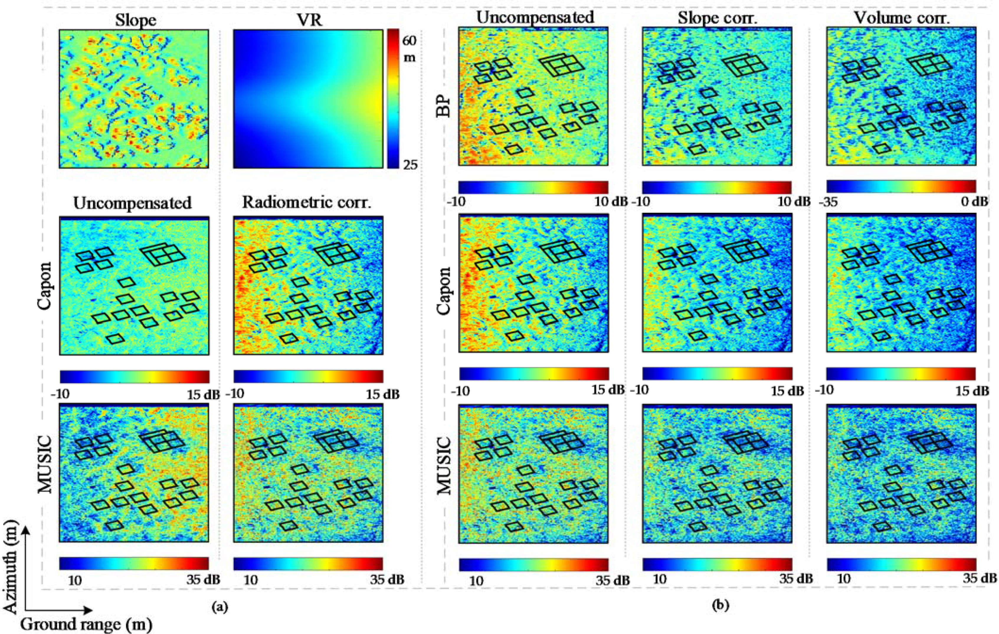
2.2. Tomographic Compensation
2.2.1. Radiometric Compensation
2.2.2. Slope Compensation
2.2.3. Volumetric Compensation
3. Materials and Methods
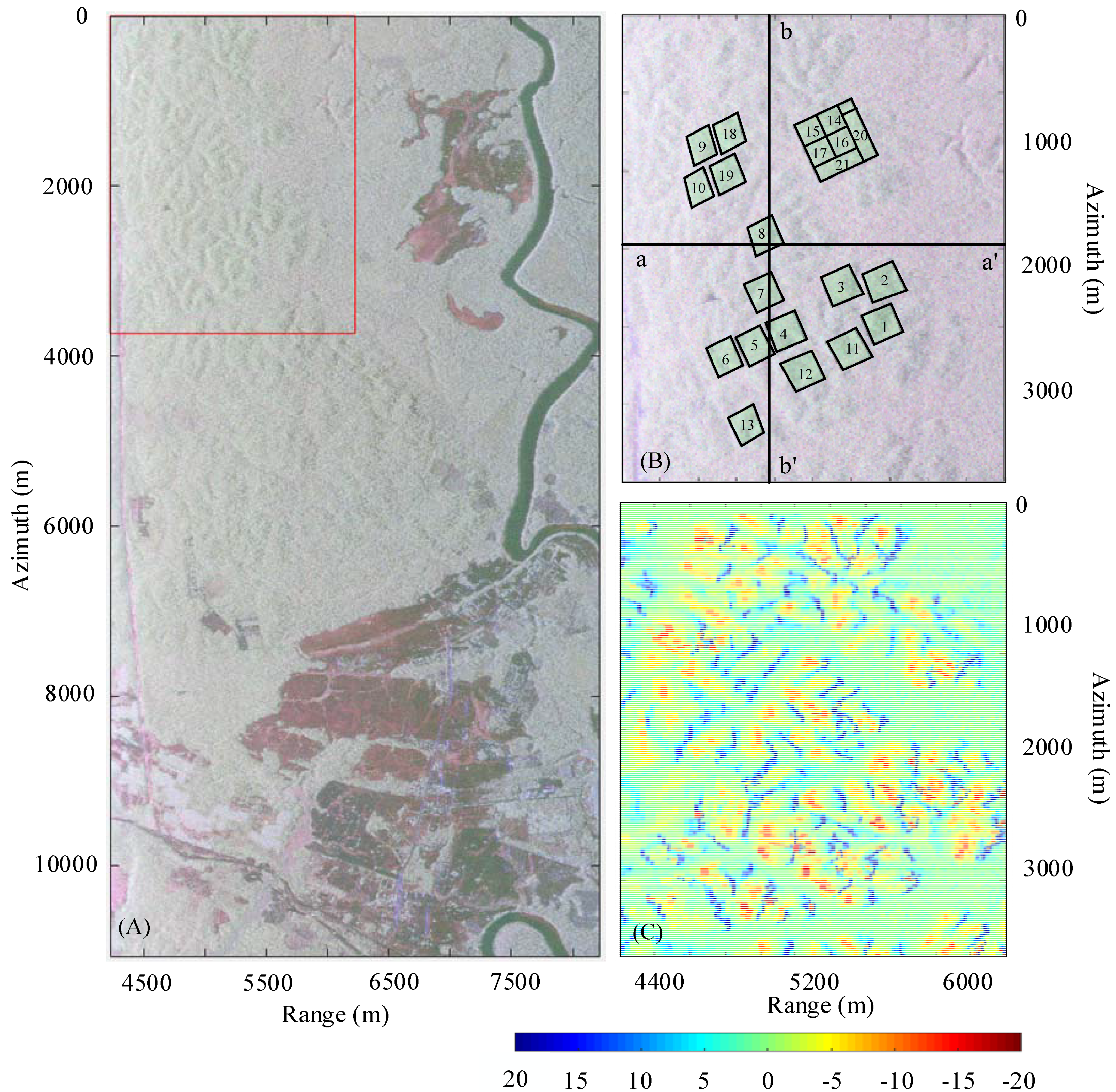
3.1. Materials
3.2. Methods
4. Results and Discussions
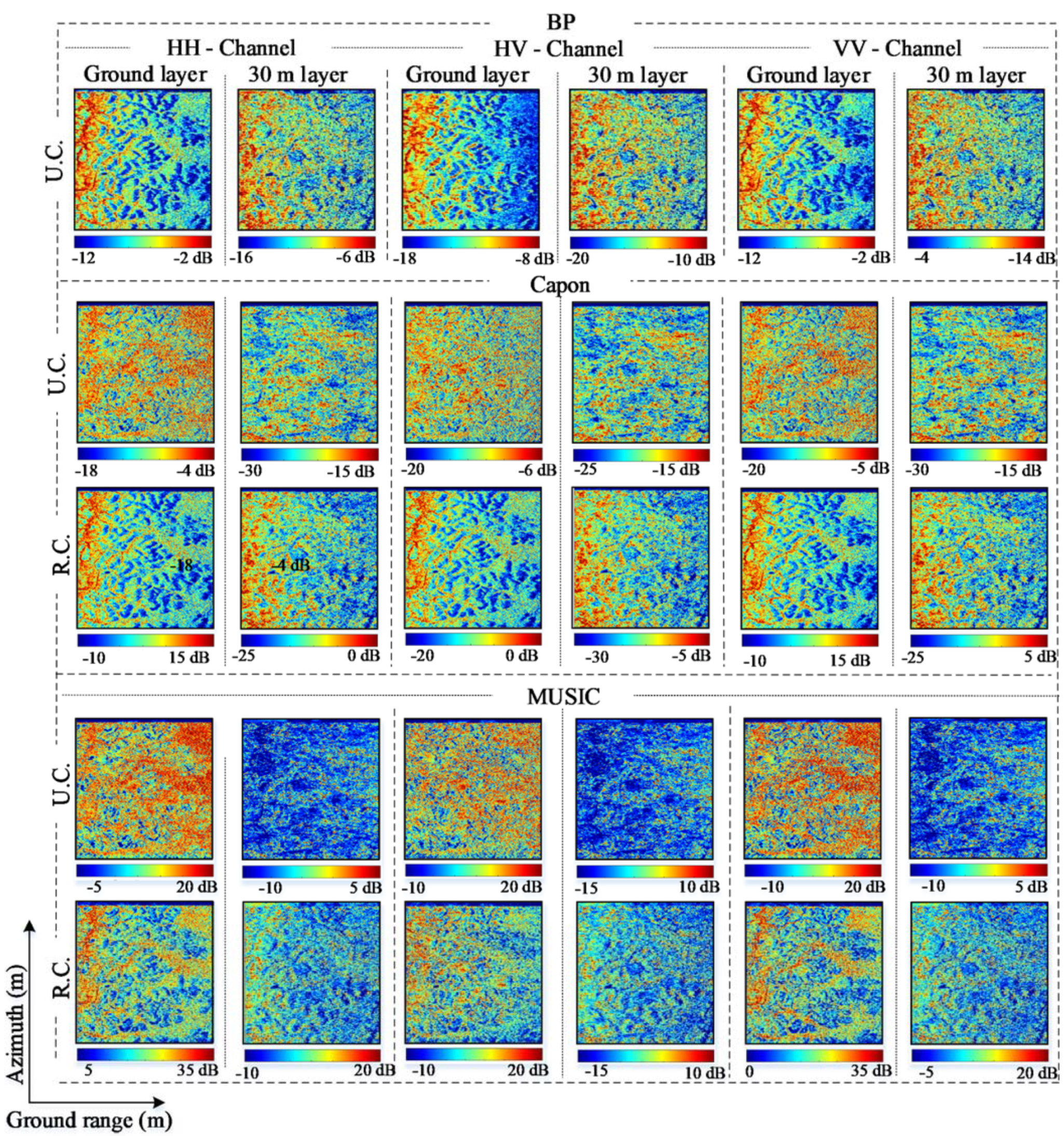
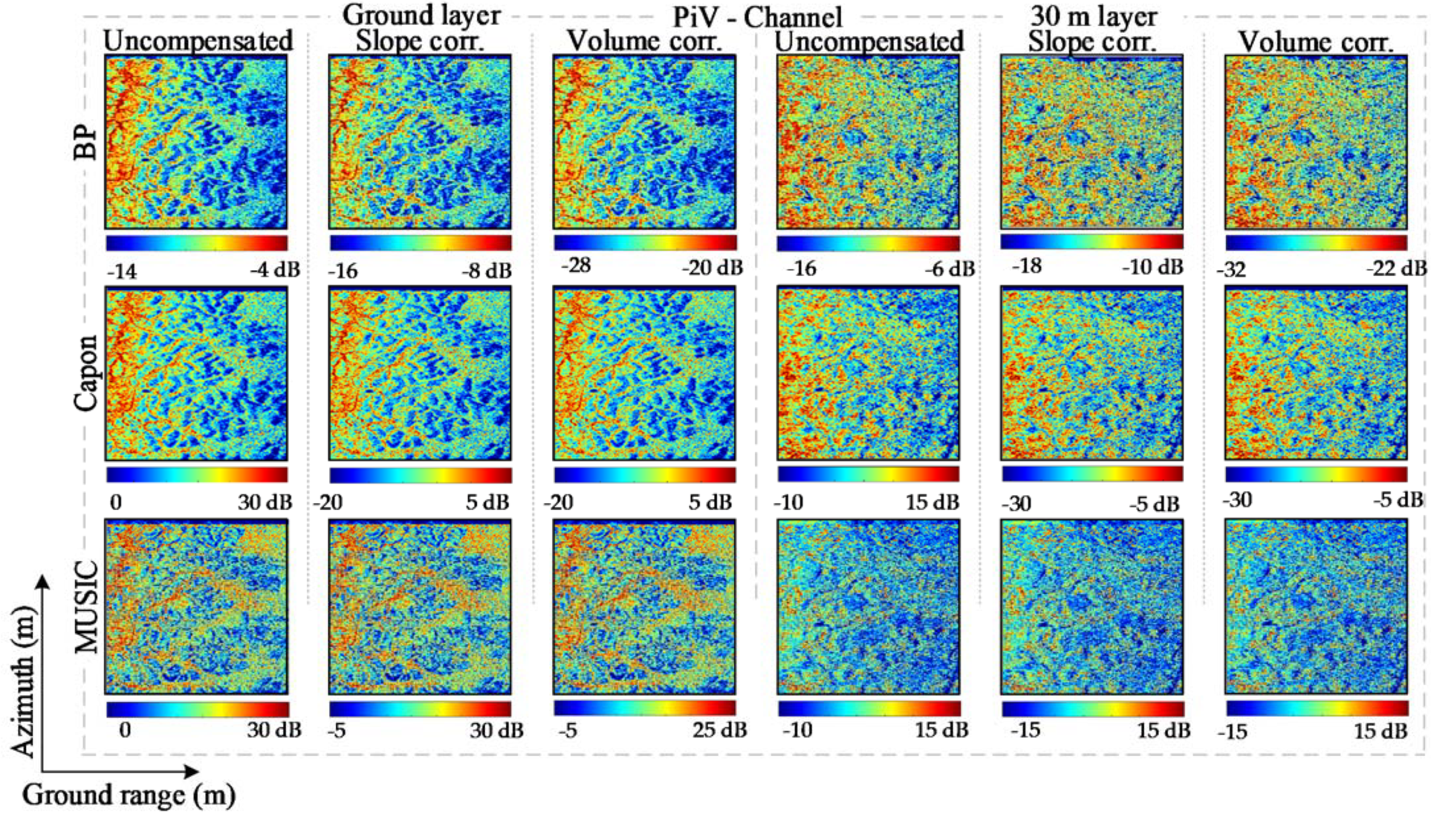
4.1. Tomographic Profile and the Multi-Layer Stack
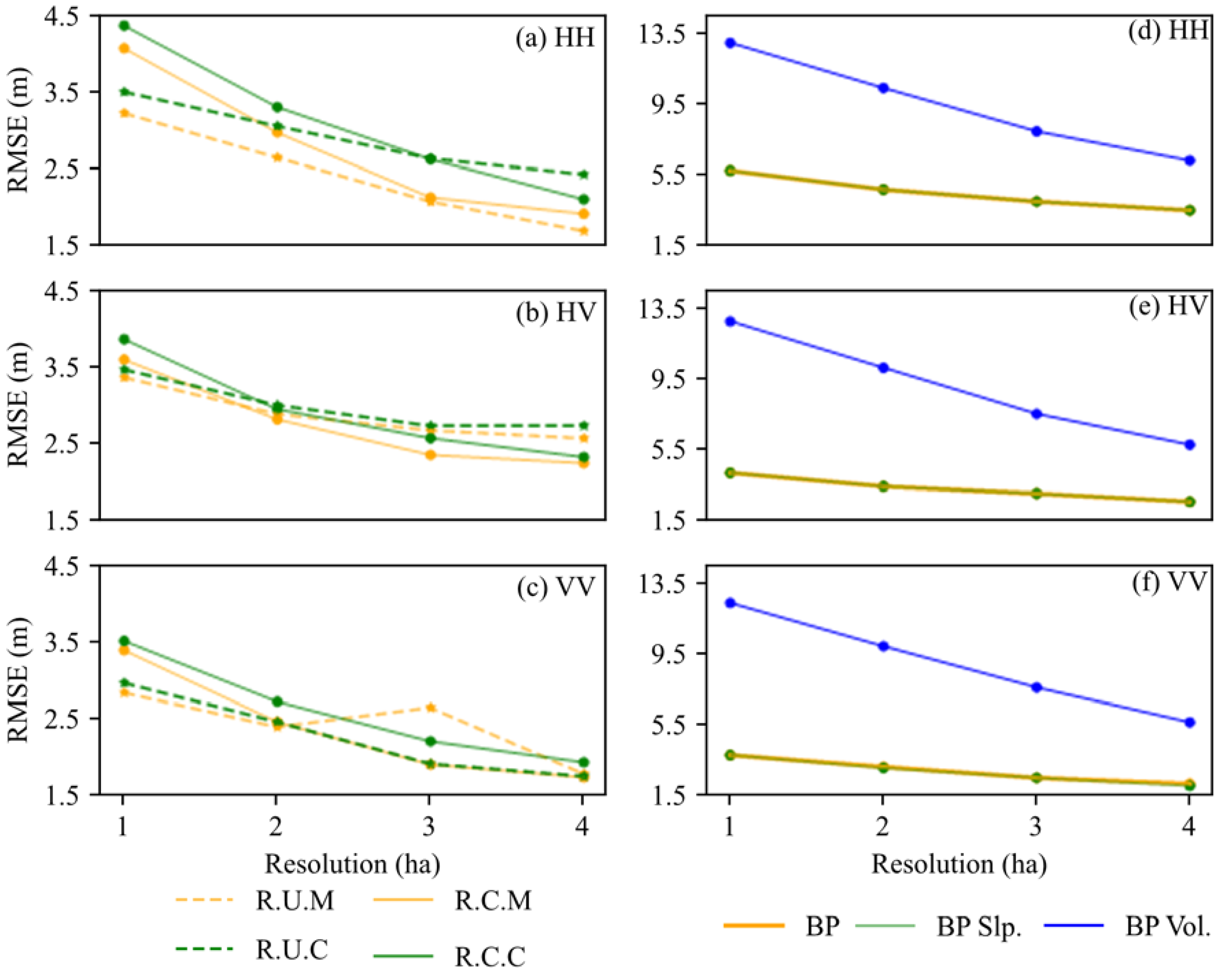
4.2. Tomographic Tree Height Estimation
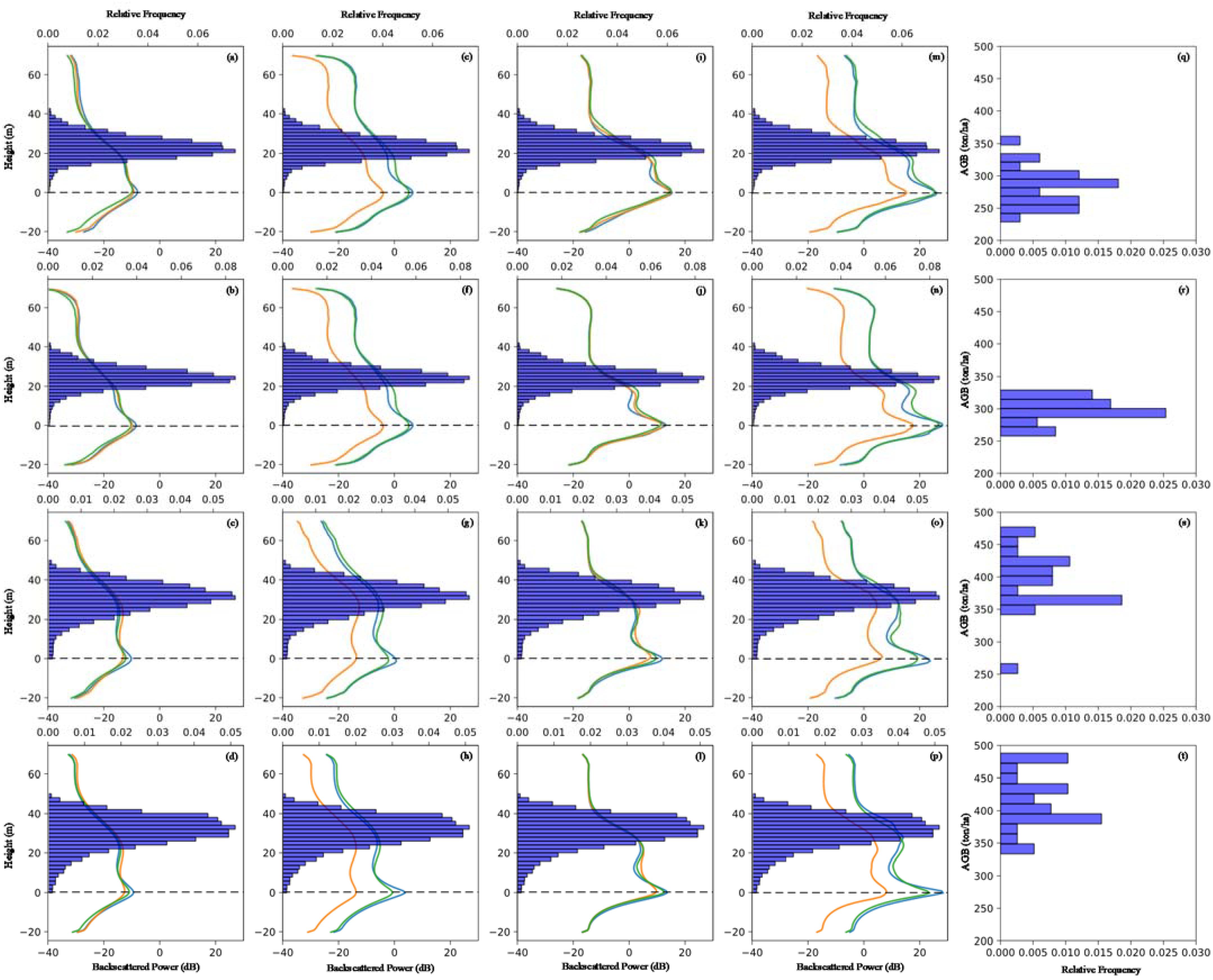
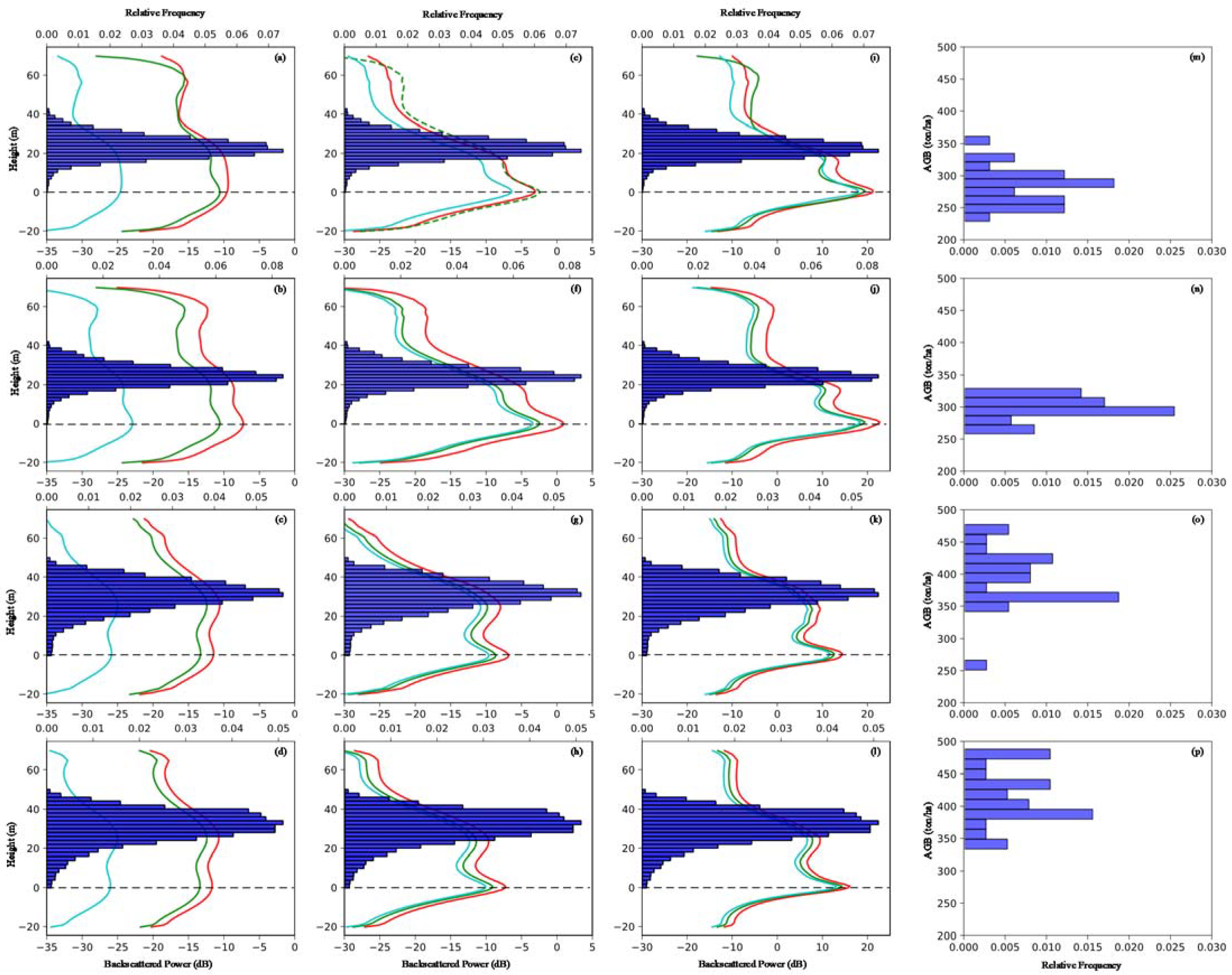
4.3. Forest Vertical Profile and Tomographic Metric
5. Conclusions
Author Contributions
Funding
Acknowledgments
Conflicts of Interest
References
- Mitchard, E.T.A. The tropical forest carbon cycle and climate change. Nature 2018, 559, 527–534. [Google Scholar] [CrossRef]
- Cramer, W.; Bondeau, A.; Schaphoff, S.; Lucht, W.; Smith, B.; Sitch, S. Tropical forests and the global carbon cycle: Impacts of atmospheric carbon dioxide, climate change and rate of deforestation. Philos. Trans. R. Soc. Lond. Ser. B Biol. Sci. 2004, 359, 331–343. [Google Scholar] [CrossRef] [PubMed] [Green Version]
- Liang, S.; Wang, J. Advanced Remote Sensing: Terrestrial Information Extraction and Applications, 2nd ed.; Liang, S.N., Wang, J., Eds.; Academic Press: London, UK, 2020; ISBN 9780128158265. [Google Scholar]
- Spies, T.A. Forest Structure: A Key to the Ecosystem. Northwest Sci. 1998, 72, 34–36. [Google Scholar]
- Bongers, F. Methods to assess tropical rain forest canopy structure: An overview. Plant Ecol. 2001, 153, 263–277. [Google Scholar] [CrossRef]
- Giri, C.; Pengra, B.; Zhu, Z.; Singh, A.; Tieszen, L.L. Monitoring mangrove forest dynamics of the Sundarbans in Bangladesh and India using multi-temporal satellite data from 1973 to 2000. Estuar. Coast. Shelf Sci. 2007, 73, 91–100. [Google Scholar] [CrossRef]
- Nicotra, A.B.; Chazdon, R.L.; Iriarte, S.V.B. Spatial Heterogeneity of Light and Woody Seedling Regeneration in Tropical Wet Forests. Ecology 1999, 80, 1908–1926. [Google Scholar] [CrossRef]
- Purves, D.; Pacala, S. Predictive models of forest dynamics. Science 2008, 320, 1452–1453. [Google Scholar] [CrossRef]
- Thom, D.; Rammer, W.; Seidl, R. The impact of future forest dynamics on climate: Interactive effects of changing vegetation and disturbance regimes. Ecol. Monogr. 2017, 87, 665–684. [Google Scholar] [CrossRef] [PubMed] [Green Version]
- Pan, Y.; Birdsey, R.A.; Fang, J.; Houghton, R.; Kauppi, P.E.; Kurz, W.A.; Phillips, O.L.; Shvidenko, A.; Lewis, S.L.; Canadell, J.G.; et al. A large and persistent carbon sink in the world’s forests. Science 2011, 333, 988–993. [Google Scholar] [CrossRef] [PubMed] [Green Version]
- Mitchard, E.T.; Saatchi, S.S.; Baccini, A.; Asner, G.P.; Goetz, S.J.; Harris, N.L.; Brown, S. Uncertainty in the spatial distribution of tropical forest biomass: A comparison of pan-tropical maps. Carbon Balance Manag. 2013, 8, 10. [Google Scholar] [CrossRef] [PubMed] [Green Version]
- Aghababaei, H.; Ferraioli, G.; Ferro-Famil, L.; Huang, Y.; Mariotti d’’Alessandro, M.; Pascazio, V.; Schirinzi, G.; Tebaldini, S. Forest SAR Tomography: Principles and Applications. IEEE Geosci. Remote Sens. Mag. 2020, 8, 30–45. [Google Scholar] [CrossRef]
- Cazcarra-Bes, V.; Tello-Alonso, M.; Fischer, R.; Heym, M.; Papathanassiou, K. Monitoring of Forest Structure Dynamics by Means of L-Band SAR Tomography. Remote Sens. 2017, 9, 1229. [Google Scholar] [CrossRef] [Green Version]
- Moussawi, I.; Ho Tong Minh, D.; Baghdadi, N.; Abdallah, C.; Jomaah, J.; Strauss, O.; Lavalle, M.; Ngo, Y.-N. Monitoring Tropical Forest Structure Using SAR Tomography at L- and P-Band. Remote Sens. 2019, 11, 1934. [Google Scholar] [CrossRef] [Green Version]
- Reigber, A.; Moreira, A. First demonstration of airborne SAR tomography using multibaseline L-band data. IEEE Trans. Geosci. Remote Sens. 2000, 38, 2142–2152. [Google Scholar] [CrossRef]
- Tebaldini, S. Single and Multipolarimetric SAR Tomography of Forested Areas: A Parametric Approach. IEEE Trans. Geosci. Remote Sens. 2010, 48, 2375–2387. [Google Scholar] [CrossRef]
- Ho Tong Minh, D.; Le Toan, T.; Rocca, F.; Tebaldini, S.; Villard, L.; Réjou-Méchain, M.; Phillips, O.L.; Feldpausch, T.R.; Dubois-Fernandez, P.; Scipal, K.; et al. SAR tomography for the retrieval of forest biomass and height: Cross-validation at two tropical forest sites in French Guiana. Remote Sens. Environ. 2016, 175, 138–147. [Google Scholar] [CrossRef] [Green Version]
- Cloude, S.R. Polarization coherence tomography. Radio Sci. 2006, 41. [Google Scholar] [CrossRef]
- Treuhaft, R.N.; Madsen, S.N.; Moghaddam, M.; van Zyl, J.J. Vegetation characteristics and underlying topography from interferometric radar. Radio Sci. 1996, 31, 1449–1485. [Google Scholar] [CrossRef]
- Treuhaft, R.N.; Siqueira, P.R. Vertical structure of vegetated land surfaces from interferometric and polarimetric radar. Radio Sci. 2000, 35, 141–177. [Google Scholar] [CrossRef] [Green Version]
- Papathanassiou, K.P.; Cloude, S.R. Single-baseline polarimetric SAR interferometry. IEEE Trans. Geosci. Remote Sens. 2001, 39, 2352–2363. [Google Scholar] [CrossRef] [Green Version]
- Pasquali, P.; Prati, C.; Rocca, F.; Seymour, M.; Fortuny, J.; Ohlmer, E.; Sieber, A.J. A 3-D SAR experiment with EMSL data. In Quantitative Remote Sensing for Science and Applications, Proceedings of the 1995 International Geoscience and Remote Sensing Symposium, Congress Center, Firenze, Italy, 10–14 July 1995; IGARSS 95, Quantitative Remote Sensing for Science and Applications; Institute of Electrical and Electronics Engineers, IEEE Service Center: New York, NY, USA; Piscataway, NJ, USA, 1995; ISBN 0780325672. [Google Scholar]
- Huang, Y.; Ferro-Famil, L.; Reigber, A. Under-Foliage Object Imaging Using SAR Tomography and Polarimetric Spectral Estimators. IEEE Trans. Geosci. Remote Sens. 2012, 50, 2213–2225. [Google Scholar] [CrossRef] [Green Version]
- Gini, F.; Lombardini, F.; Montanari, M. Layover solution in multibaseline SAR interferometry. IEEE Trans. Aerosp. Electron. Syst. 2002, 38, 1344–1356. [Google Scholar] [CrossRef]
- Lombardini, F.; Reigber, A. Adaptive spectral estimation for multibaseline SAR tomography with airborne L-band data. In Proceedings of the IGARSS 2003 IEEE International Geoscience and Remote Sensing Symposium. (IEEE Cat. No.03CH37477), Toulouse, France, 21–25 July 2003; pp. 2014–2016, ISBN 0-7803-7929-2. [Google Scholar]
- Fornaro, G.; Serafino, F.; Soldovieri, F. Three-dimensional focusing with multipass SAR data. IEEE Trans. Geosci. Remote Sens. 2003, 41, 507–517. [Google Scholar] [CrossRef]
- Tebaldini, S. Forest SAR tomography: A covariance matching approach. In Proceedings of the 2008 IEEE Radar Conference, Rome, Italy, 26–30 May 2008; ISBN 9781424415380.
- Tebaldini, S.; Rocca, F. Multibaseline Polarimetric SAR Tomography of a Boreal Forest at P- and L-Bands. IEEE Trans. Geosci. Remote Sens. 2012, 50, 232–246. [Google Scholar] [CrossRef]
- Nannini, M.; Scheiber, R.; Moreira, A. Estimation of the Minimum Number of Tracks for SAR Tomography. IEEE Trans. Geosci. Remote Sens. 2009, 47, 531–543. [Google Scholar] [CrossRef]
- Aguilera, E.; Nannini, M.; Reigber, A. A Data-Adaptive Compressed Sensing Approach to Polarimetric SAR Tomography of Forested Areas. IEEE Geosci. Remote Sens. Lett. 2013, 10, 543–547. [Google Scholar] [CrossRef]
- Zhu, X.X.; Bamler, R. Demonstration of Super-Resolution for Tomographic SAR Imaging in Urban Environment. IEEE Trans. Geosci. Remote Sens. 2012, 50, 3150–3157. [Google Scholar] [CrossRef] [Green Version]
- Aguilera, E.; Nannini, M.; Reigber, A. Wavelet-Based Compressed Sensing for SAR Tomography of Forested Areas. IEEE Trans. Geosci. Remote Sens. 2013, 51, 5283–5295. [Google Scholar] [CrossRef] [Green Version]
- Aguilera, E.; Nannini, M.; Reigber, A. Multi-signal compressed sensing for polarimetric SAR tomography. In Proceedings of the 2011 IEEE International Geoscience and Remote Sensing Symposium, Sendai, Japan, 1–5 August 2011; pp. 1369–1372, ISBN 2153-7003. [Google Scholar]
- Freeman, A.; Saatchi, S.S. On the detection of Faraday rotation in linearly polarized L-band SAR backscatter signatures. IEEE Trans. Geosci. Remote Sens. 2004, 42, 1607–1616. [Google Scholar] [CrossRef]
- Rogers, N.C.; Quegan, S.; Kim, J.S.; Papathanassiou, K.P. Impacts of Ionospheric Scintillation on the BIOMASS P-Band Satellite SAR. IEEE Trans. Geosci. Remote Sens. 2014, 52, 1856–1868. [Google Scholar] [CrossRef] [Green Version]
- Mariotti d’Alessandro, M.; Tebaldini, S. Phenomenology of P-Band Scattering from a Tropical Forest Through Three-Dimensional SAR Tomography. IEEE Geosci. Remote Sens. Lett. 2012, 9, 442–446. [Google Scholar] [CrossRef]
- Mariotti d’Alessandro, M.; Tebaldini, S. Phenomenology of Ground Scattering in a Tropical Forest through Polarimetric Synthetic Aperture Radar Tomography. IEEE Trans. Geosci. Remote Sens. 2013, 51, 4430–4437. [Google Scholar] [CrossRef]
- Bamler, R.; Philipp, H. Synthetic aperture radar interferometry. Inverse Probl. 1998, 14, R1–R54. [Google Scholar] [CrossRef]
- Tebaldini, S.; Guarnieri, A.M. On the Role of Phase Stability in SAR Multibaseline Applications. IEEE Trans. Geosci. Remote Sens. 2010, 48, 2953–2966. [Google Scholar] [CrossRef]
- Ho Tong Minh, D.; Le Toan, T.; Rocca, F.; Tebaldini, S.; D’Alessandro, M.M.; Villard, L. Relating P-Band Synthetic Aperture Radar Tomography to Tropical Forest Biomass. IEEE Trans. Geosci. Remote Sens. 2014, 52, 967–979. [Google Scholar] [CrossRef]
- Ho Tong Minh, D.; Tebaldini, S.; Rocca, F.; Le Toan, T.; Villard, L.; Dubois-Fernandez, P.C. Capabilities of BIOMASS Tomography for Investigating Tropical Forests. IEEE Trans. Geosci. Remote Sens. 2015, 53, 965–975. [Google Scholar] [CrossRef]
- Lombardini, F.; Cai, F.; Viviani, F.; Pasculli, D. Multidimensional SAR tomography for complex non-stationary scenes: COSMO-SkyMed urban and P-band forest results. In Proceedings of the IEEE International Geoscience and Remote Sensing Symposium (IGARSS), Munich, Germany, 22–27 July 2012; IEEE: Piscataway, NJ, USA, 2012; pp. 5206–5209. ISBN 978-1-4673-1159-5. [Google Scholar]
- Nannini, M.; Scheiber, R. Height dependent motion compensation and coregistration for airborne SAR tomography. In Proceedings of the 2007 IEEE International Geoscience and Remote Sensing Symposium, Barcelona, Spain, 23–27 July 2007; IEEE: Piscataway, NJ, USA, 2007; pp. 5041–5044. ISBN 978-1-4244-1211-2. [Google Scholar]
- Nannini, M.; Scheiber, R.; Horn, R.; Moreira, A. First 3-D Reconstructions of Targets Hidden Beneath Foliage by Means of Polarimetric SAR Tomography. IEEE Geosci. Remote Sens. Lett. 2012, 9, 60–64. [Google Scholar] [CrossRef] [Green Version]
- Chen, Z.; Gokeda, G.; Yu, Y. Introduction to Direction-Of-Arrival Estimation; Artech House: Boston, MA, USA, 2010; ISBN 1596930896. [Google Scholar]
- Stoica, P.; Moses, R.L. Spectral Analysis of Signals; Pearson/Prentice Hall: Upper Saddle River, NJ, USA, 2004; ISBN 0131139568. [Google Scholar]
- Krim, H.; Viberg, M. Two decades of array signal processing research: The parametric approach. IEEE Signal Process. Mag. 1996, 13, 67–94. [Google Scholar] [CrossRef]
- Saatchi, S.S.; van Zyl, J.J.; Asrar, G. Estimation of canopy water content in Konza Prairie grasslands using synthetic aperture radar measurements during FIFE. J. Geophys. Res. 1995, 100, 25481. [Google Scholar] [CrossRef]
- van Zyl, J.J.; Chapman, B.D.; Dubois, P.; Shi, J. The effect of topography on SAR calibration. IEEE Trans. Geosci. Remote Sens. 1993, 31, 1036–1043. [Google Scholar] [CrossRef]
- Molto, Q.; Rossi, V.; Blanc, L. Error propagation in biomass estimation in tropical forests. Methods Ecol Evol 2013, 4, 175–183. [Google Scholar] [CrossRef]
- Chave, J.; Piponiot, C.; Maréchaux, I.; Foresta, H.D.; Larpin, D.; Fischer, F.J.; Derroire, G.; Vincent, G.; Hérault, B. Slow rate of secondary forest carbon accumulation in the Guianas compared with the rest of the Neotropics. Ecol. Appl. 2020, 30, e02004. [Google Scholar] [CrossRef]
- Labriere, N.; Tao, S.; Chave, J.; Scipal, K.; Le Toan, T.; Abernethy, K.; Alonso, A.; Barbier, N.; Bissiengou, P.; Casal, T.; et al. In Situ Reference Datasets from the TropiSAR and AfriSAR Campaigns in Support of Upcoming Spaceborne Biomass Missions. IEEE J. Sel. Top. Appl. Earth Obs. Remote Sens. 2018, 11, 3617–3627. [Google Scholar] [CrossRef]
- Reigber, A.; Prats, P.; Mallorqui, J.J. Refined Estimation of Time-Varying Baseline Errors in Airborne SAR Interferometry. IEEE Geosci. Remote Sens. Lett. 2006, 3, 145–149. [Google Scholar] [CrossRef]
- Tebaldini, S.; Rocca, F. On the impact of propagation disturbances on SAR Tomography: Analysis and compensation. In Proceedings of the 2009 IEEE Radar Conference, Pasadena, CA, USA, 4–8 May 2009; 2009; pp. 1–6, ISBN 978-1-4244-2870-0. [Google Scholar]
- Tebaldini, S.; Rocca, F.; Mariotti d’Alessandro, M.; Ferro-Famil, L. Phase Calibration of Airborne Tomographic SAR Data via Phase Center Double Localization. IEEE Trans. Geosci. Remote Sens. 2016, 54, 1775–1792. [Google Scholar] [CrossRef]
- Mariotti d’Alessandro, M.; Tebaldini, S. Digital Terrain Model Retrieval in Tropical Forests through P-Band SAR Tomography. IEEE Trans. Geosci. Remote Sens. 2019, 57, 6774–6781. [Google Scholar] [CrossRef]


| Polarization | BP RMSE (Power loss, rp) | Capon RMSE (Power loss, rp) | MUSIC RMSE (Power loss, rp) |
|---|---|---|---|
| HH | 3.54 (−3.75, 0.983) | 2.11 (−11.5, 0.994) | 1.92 (−18.75, 0.995) |
| HV | 2.59 (−2.5, 0.991) | 2.33 (−9.25, 0.992) | 2.25 (−16.5, 0.993) |
| VV | 2.19 (−2.25, 0.993) | 1.94 (−9.5, 0.994) | 1.74 (−17.0, 0.995) |
| PiH | 3.51 (−3.5, 0.983) | 2.54 (−11.0, 0.991) | 2.31 (−18.5, 0.992) |
| PiV | 2.27 (−2.5, 0.993) | 2.06 (−9.25, 0.994) | 1.71 (−16.75, 0.996) |
| RH | 2.86 (−3.25, 0.989) | 1.92 (−10.75, 0.995) | 1.77 (−18.25, 0.995) |
| RV | 2.11 (−2.5, 0.994) | 2.13 (−9.75, 0.994) | 1.86 (−17.25, 0.995) |
| RR | 3.02 (−3.5, 0.987) | 1.89 (−11.0, 0.995) | 1.79 (−18.75, 0.995) |
| RL | 2.3 (−2.25, 0.993) | 1.91 (−925, 0.995) | 1.77 (−17.0, 0.995) |
Publisher’s Note: MDPI stays neutral with regard to jurisdictional claims in published maps and institutional affiliations. |
© 2021 by the authors. Licensee MDPI, Basel, Switzerland. This article is an open access article distributed under the terms and conditions of the Creative Commons Attribution (CC BY) license (http://creativecommons.org/licenses/by/4.0/).
Share and Cite
Ramachandran, N.; Saatchi, S.; Tebaldini, S.; d’Alessandro, M.M.; Dikshit, O. Evaluation of P-Band SAR Tomography for Mapping Tropical Forest Vertical Backscatter and Tree Height. Remote Sens. 2021, 13, 1485. https://0-doi-org.brum.beds.ac.uk/10.3390/rs13081485
Ramachandran N, Saatchi S, Tebaldini S, d’Alessandro MM, Dikshit O. Evaluation of P-Band SAR Tomography for Mapping Tropical Forest Vertical Backscatter and Tree Height. Remote Sensing. 2021; 13(8):1485. https://0-doi-org.brum.beds.ac.uk/10.3390/rs13081485
Chicago/Turabian StyleRamachandran, Naveen, Sassan Saatchi, Stefano Tebaldini, Mauro Mariotti d’Alessandro, and Onkar Dikshit. 2021. "Evaluation of P-Band SAR Tomography for Mapping Tropical Forest Vertical Backscatter and Tree Height" Remote Sensing 13, no. 8: 1485. https://0-doi-org.brum.beds.ac.uk/10.3390/rs13081485